
Spatiotemporal Variability of Dune Velocities and Corresponding Uncertainties, Detected from Optical Image Matching in the North Sinai Sand Sea, Egypt


Abstract
:
1. Introduction
2. Study Area and Data
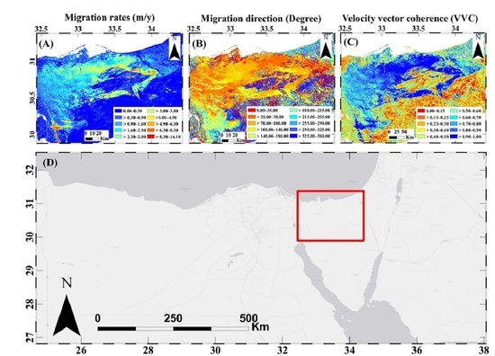
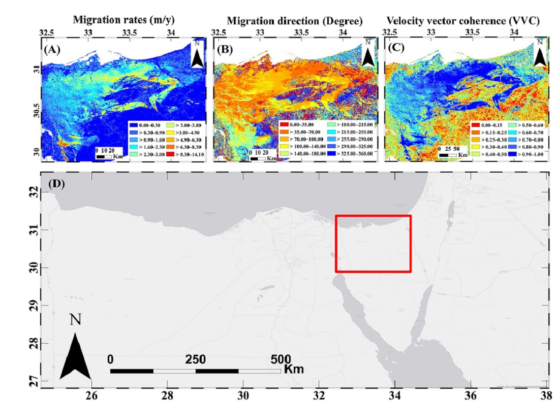
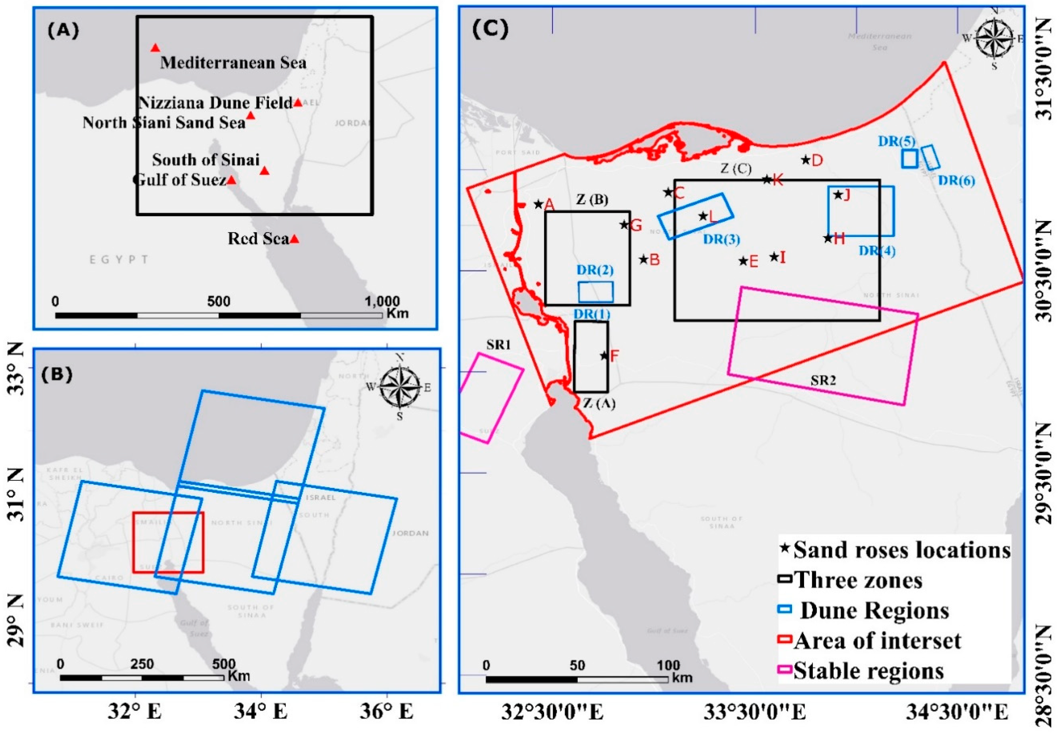
2.1. Study Area
2.2. Optical Images
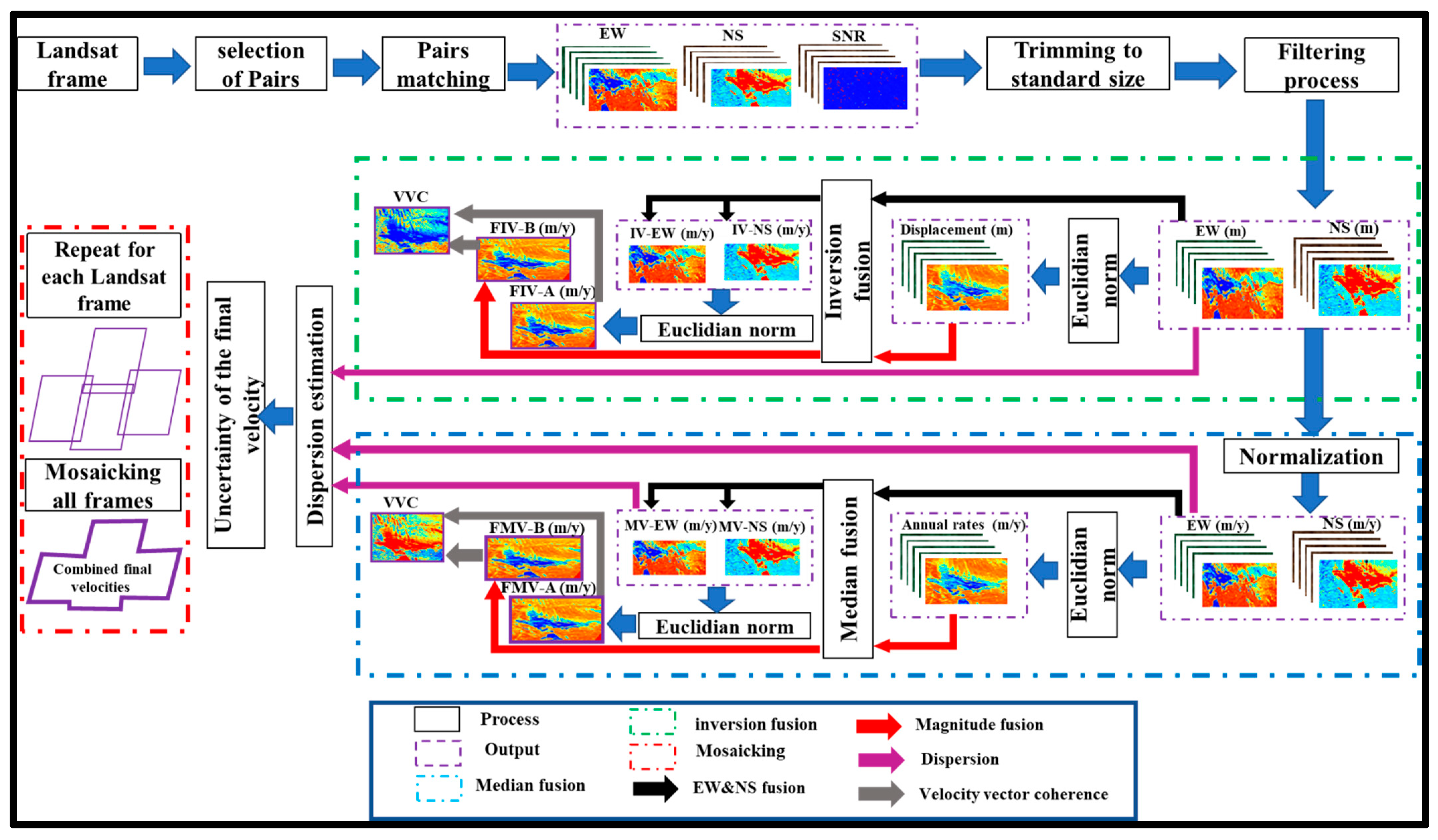
3. Methods
3.1. Pairing Formation and Matching Process
3.2. Noise Filtering and Post Processing
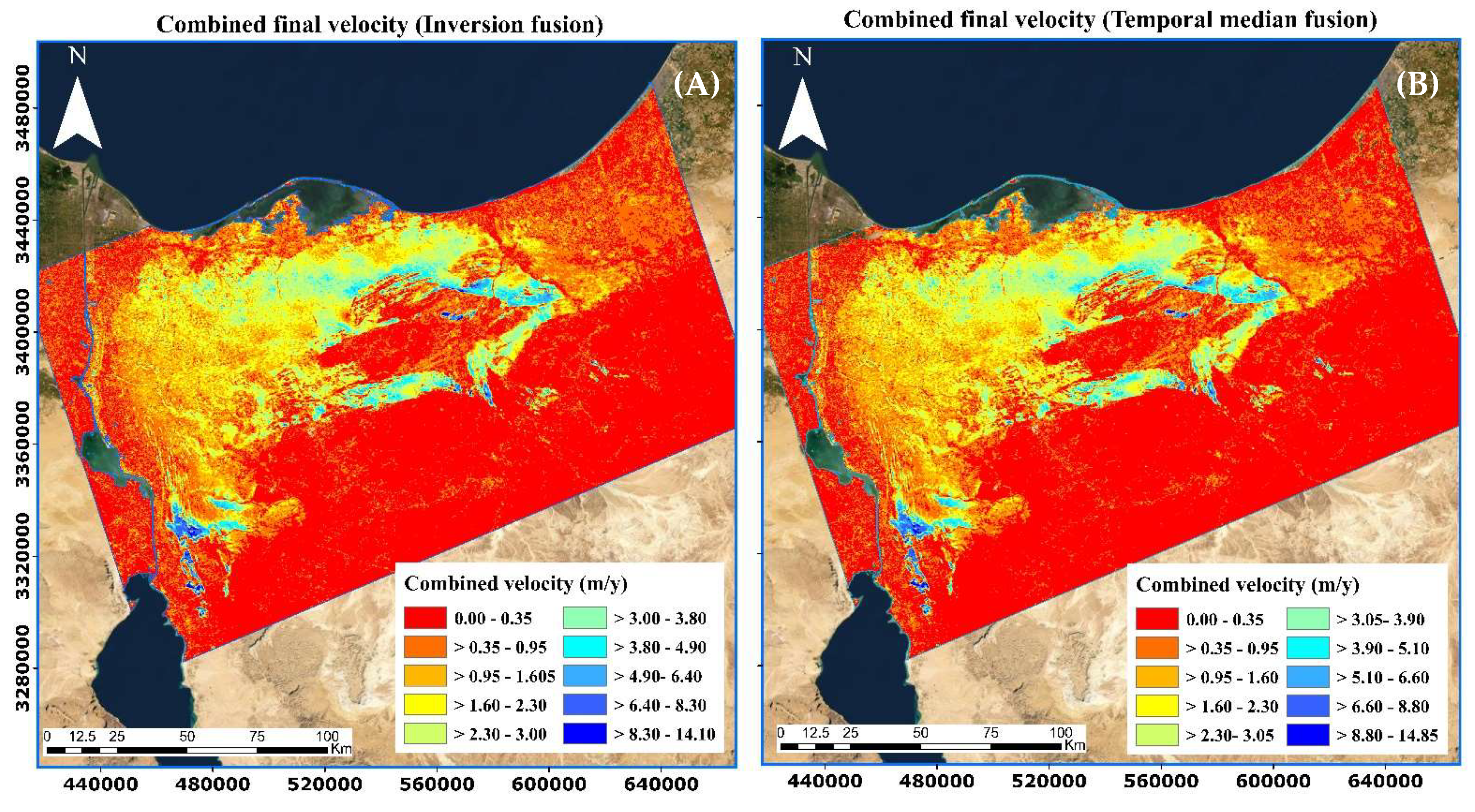
3.3. Fusion of Individual Velocites
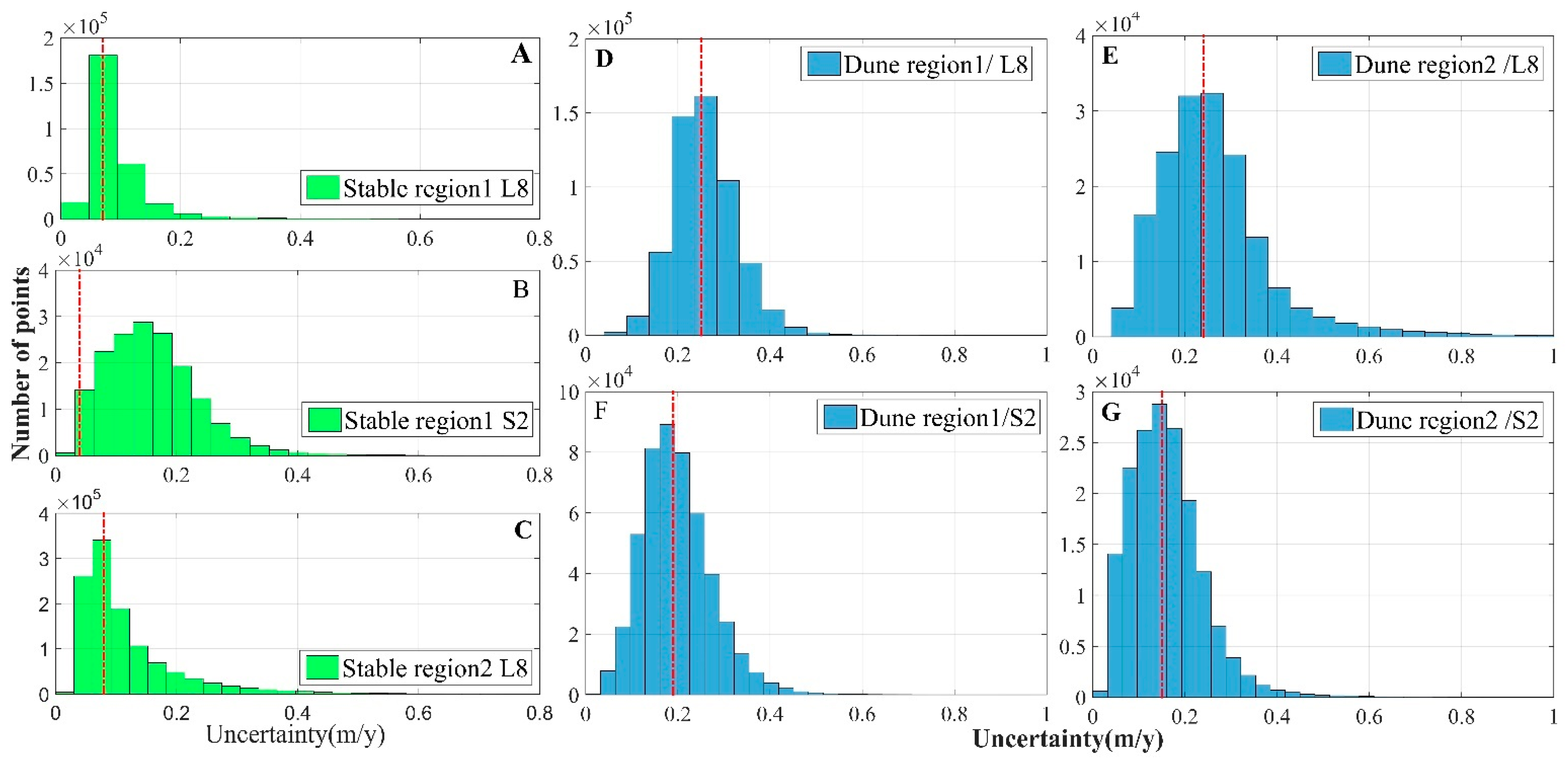
3.4. Uncertainty Estimation
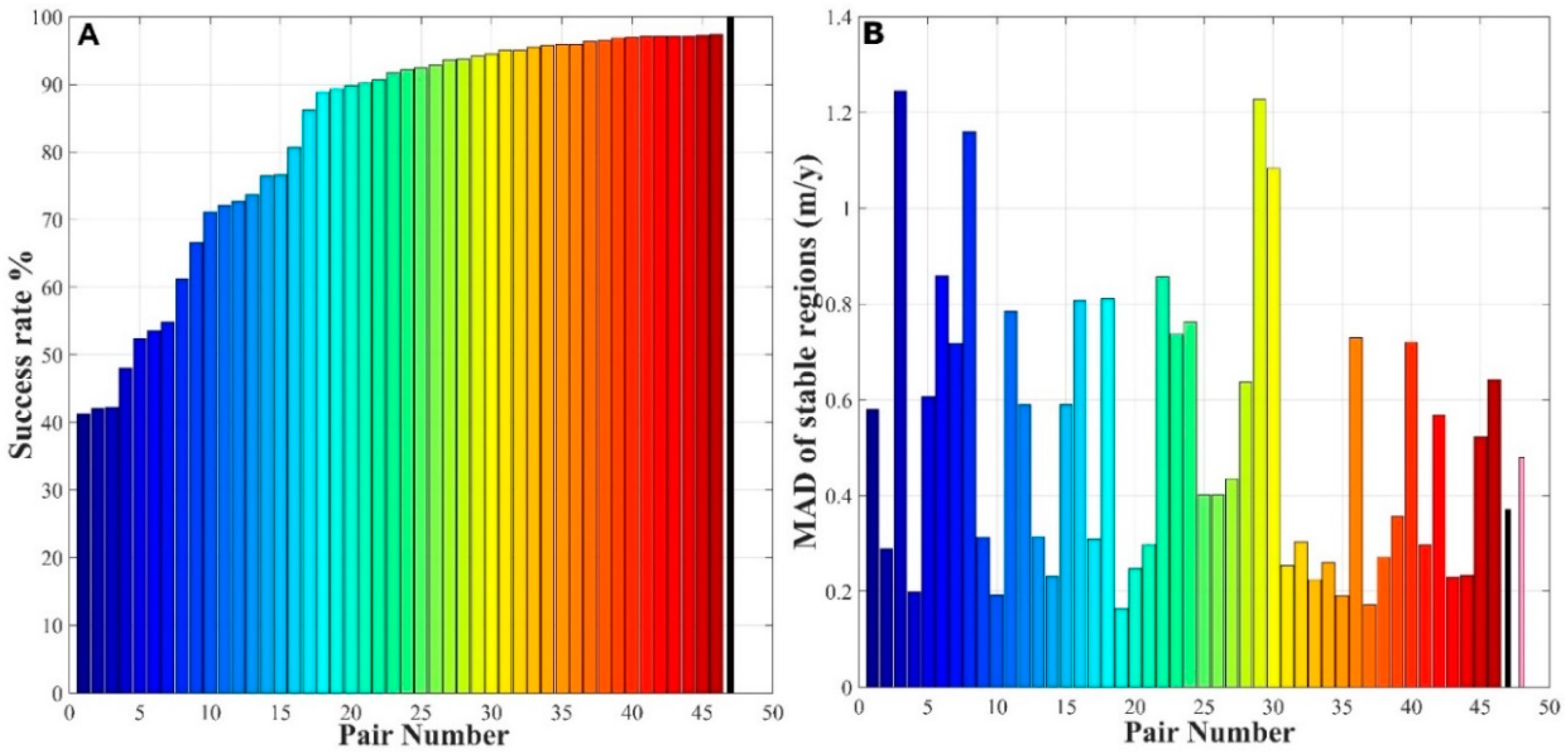
3.5. Quality Assessment and Validation
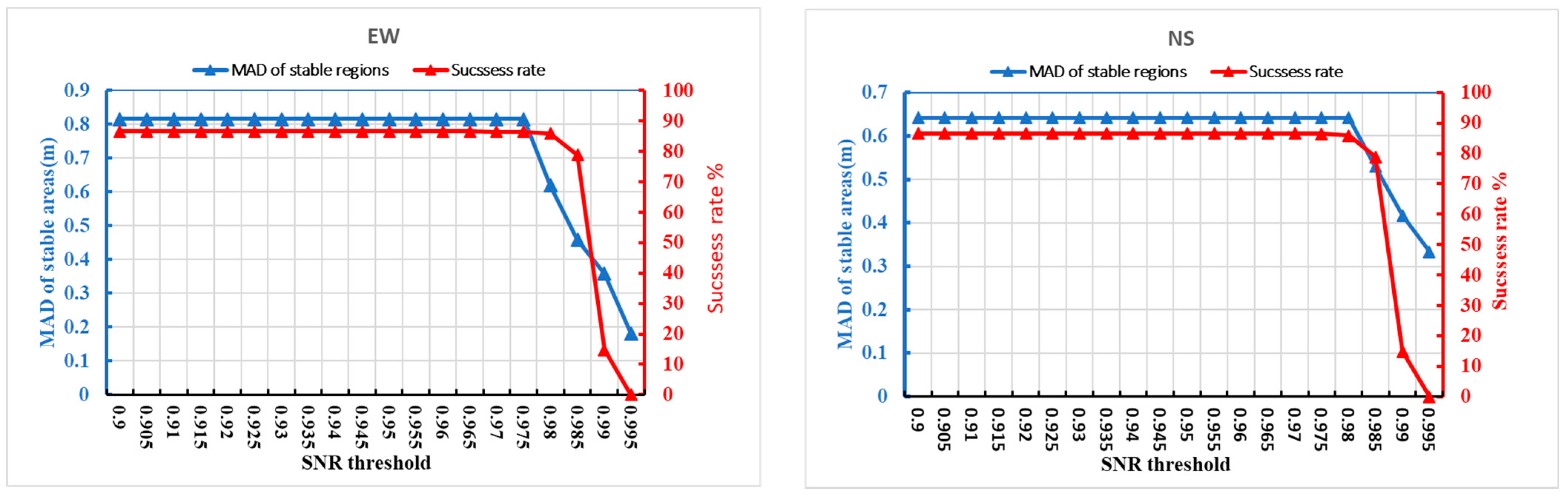
- The SR can be defined as the percentage of valid matching results on the sand dune areas. SR can be estimated by calculating the number of surviving pixels over a certain area before and after applying a certain filter [42]. We mainly used the SR to compare the performance of the SNR threshold variations on the percentages of valid matches (Section 4.1).
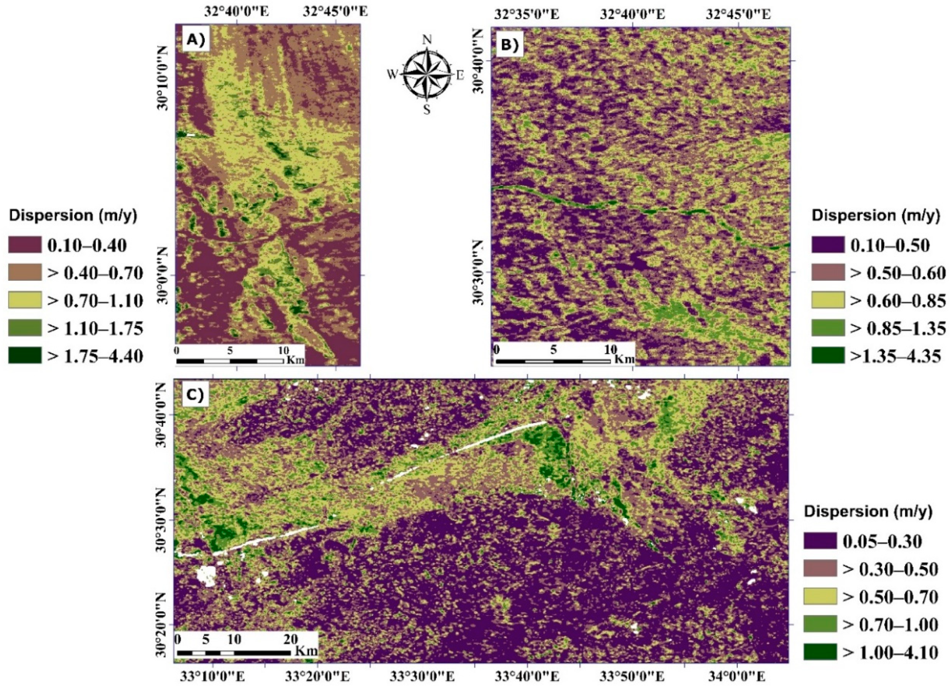
- The dispersion of the final velocity is ; dispersion is considered the measure of the difference between the estimated final velocity and all the velocities shared in generating the final velocity [42]. The dispersion can be estimated at each velocity location from Equation (5):where represents the dispersion of the final velocity. is the median of the absolute difference between each individual velocity shared to generate the final velocity and final velocity. is the total number of pairs shared in generating the final velocity in the fully stacked pixels, and is the minimum number of pairs required for a given pixel to be considered in the final velocity estimation.
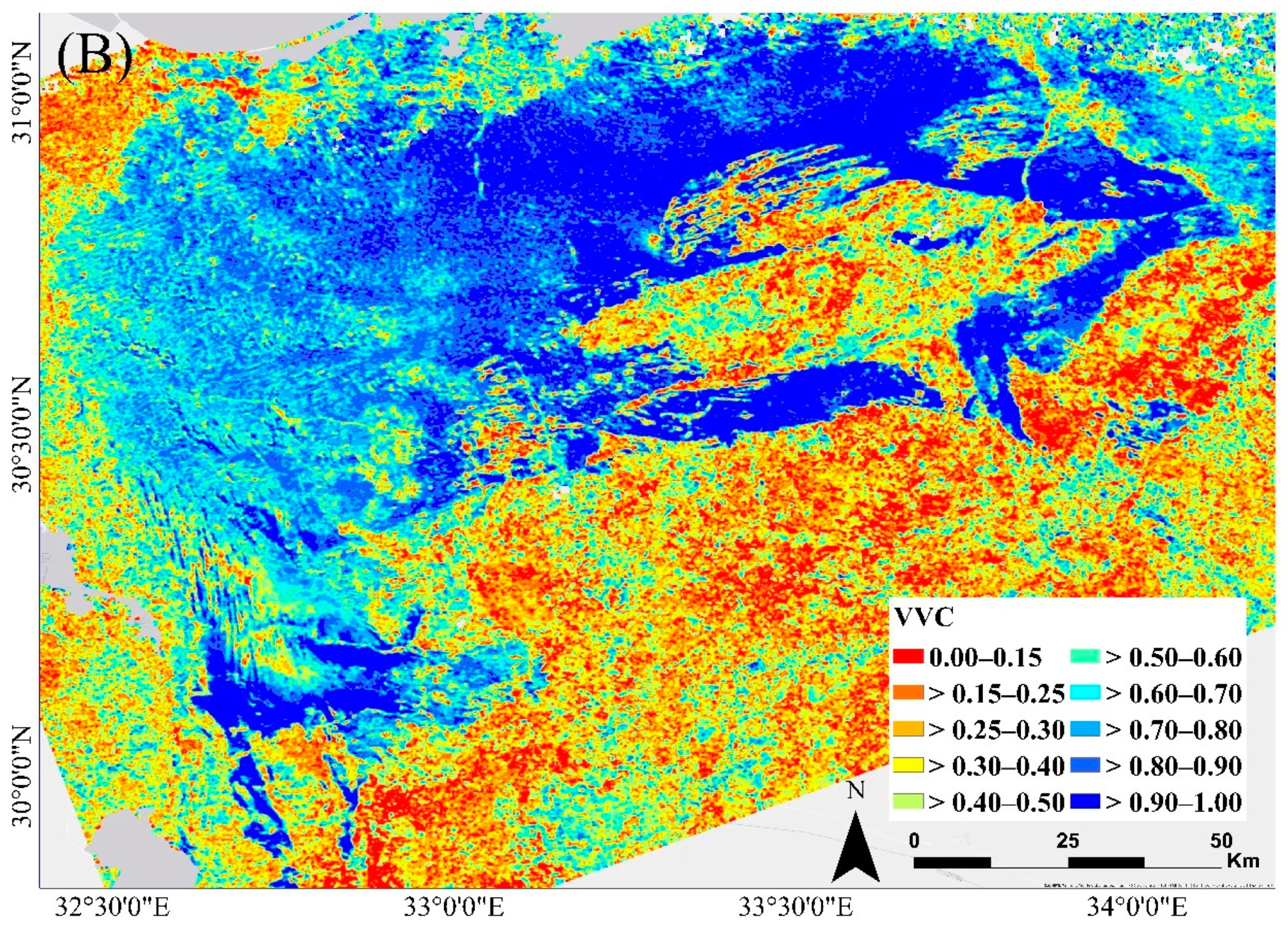
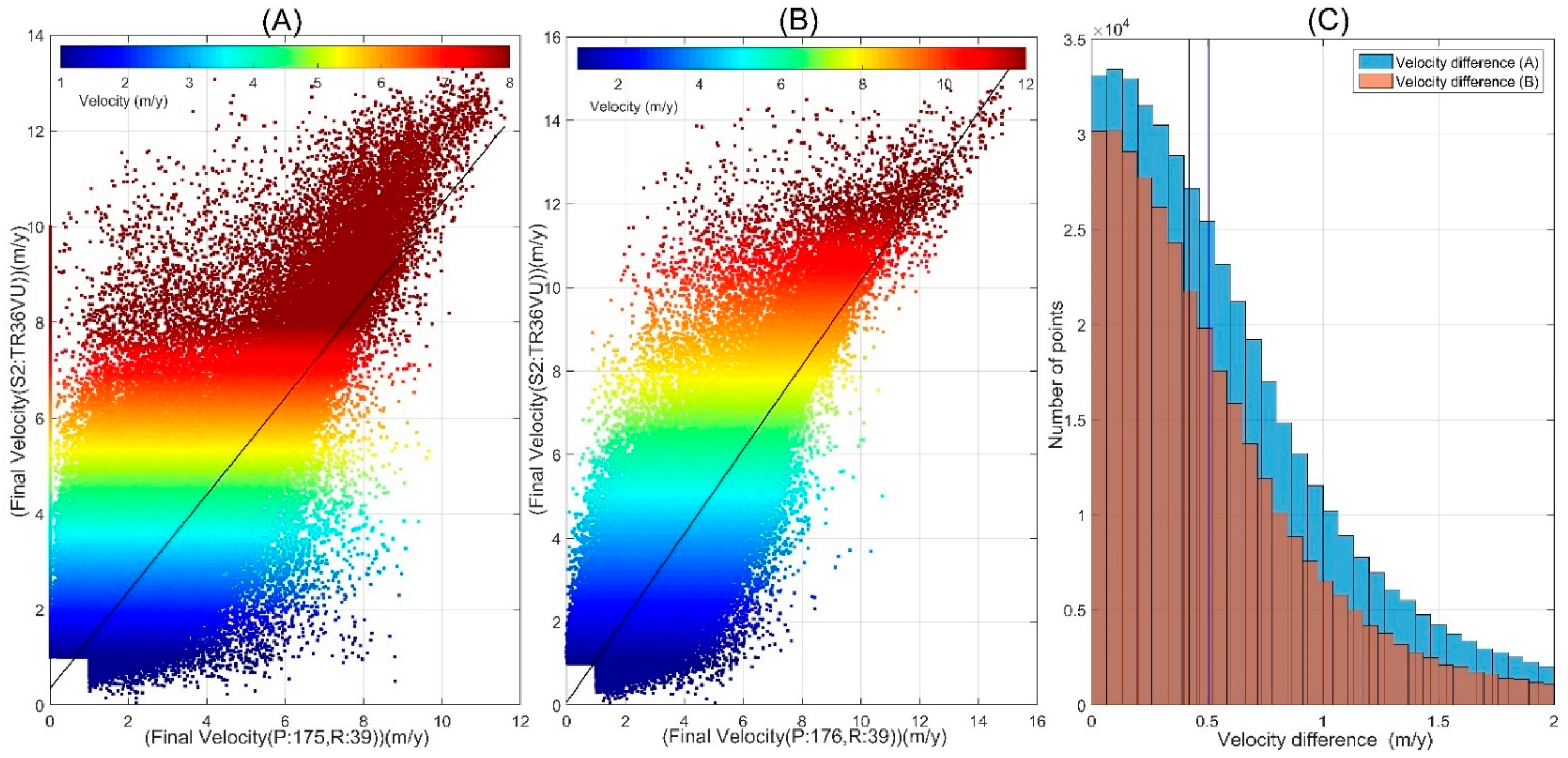
- The velocity vector coherence of the final velocity is denoted by , where the VVC is estimated for the final velocity map, representing the change in directions between the individual velocities at each velocity location [42,52]. The can be estimated from Equation (6):where The numerator in Equation (6) can be estimated at any velocity location by summing the individual velocities EW and NS and then applying the Euclidean norm. Conversely, the denominator in Equation (6) can be estimated by estimating the Euclidean norm of the two components of the velocities (i.e., EW and NS) and then summing the values of all the included velocities. According to the triangle inequality, ranges from 0 to 1, equals 1 when the directions used in estimating the final velocities are perfectly aligned, and approaches 0 when the directions are heterogeneous [42,52]. We cross-validated the Landsat-8 fusion velocities with Sentinel-2 independent fusion velocities at the overlapping locations. We also compared the final velocities extracted from the overlapping regions of adjacent Landsat-8 images. Cross-validation was performed with respect to the distribution of velocity changes between two sensors and the degree of correlation between the results at similar locations.
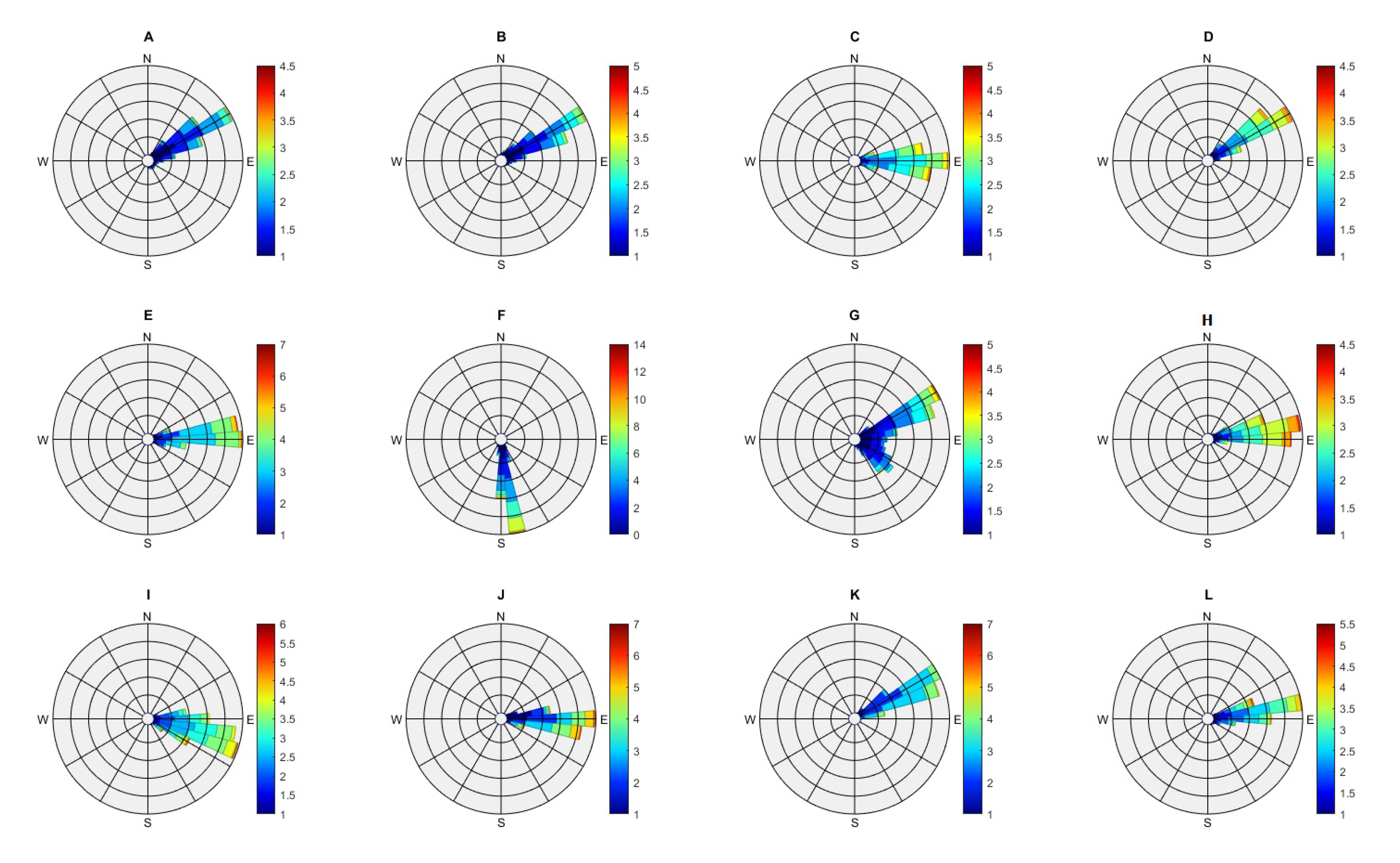
3.6. Dune Migration Directions
4. Results
4.1. Selction of SNR Thresholds
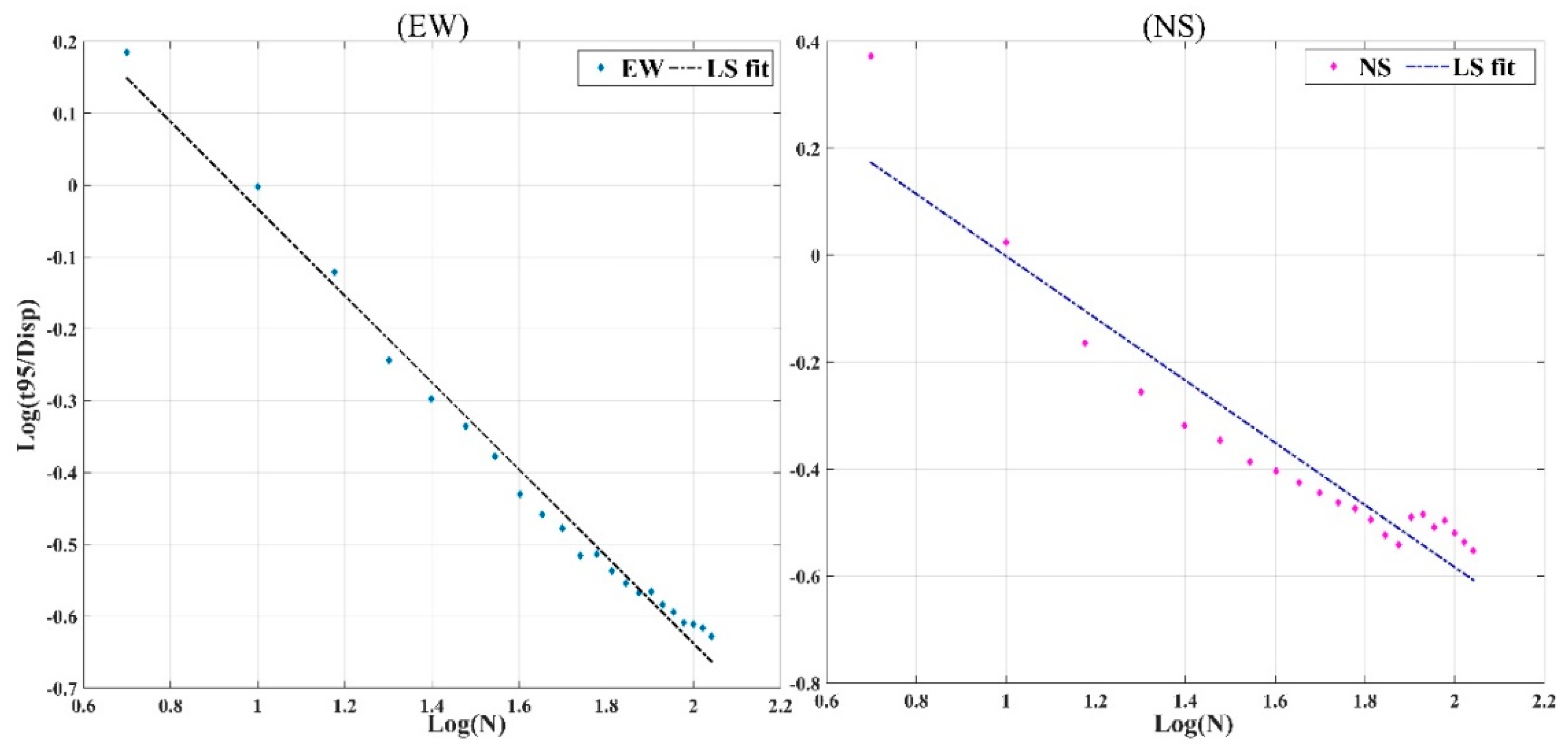
4.2. Matching Quality vs. Time Separation
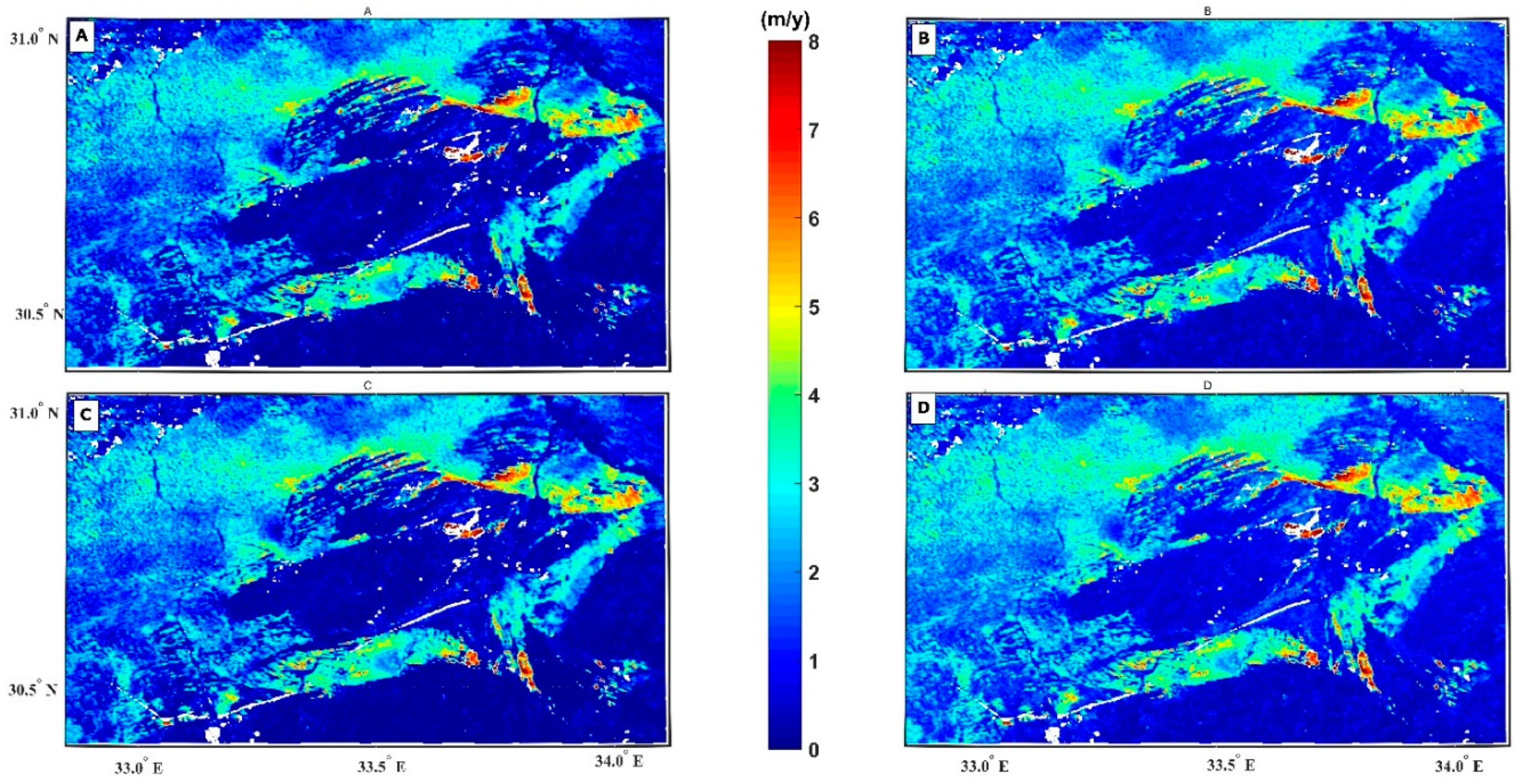
4.3. Fusion of Individual Velocites
4.4. Mosaicking of Final Velocity Fields
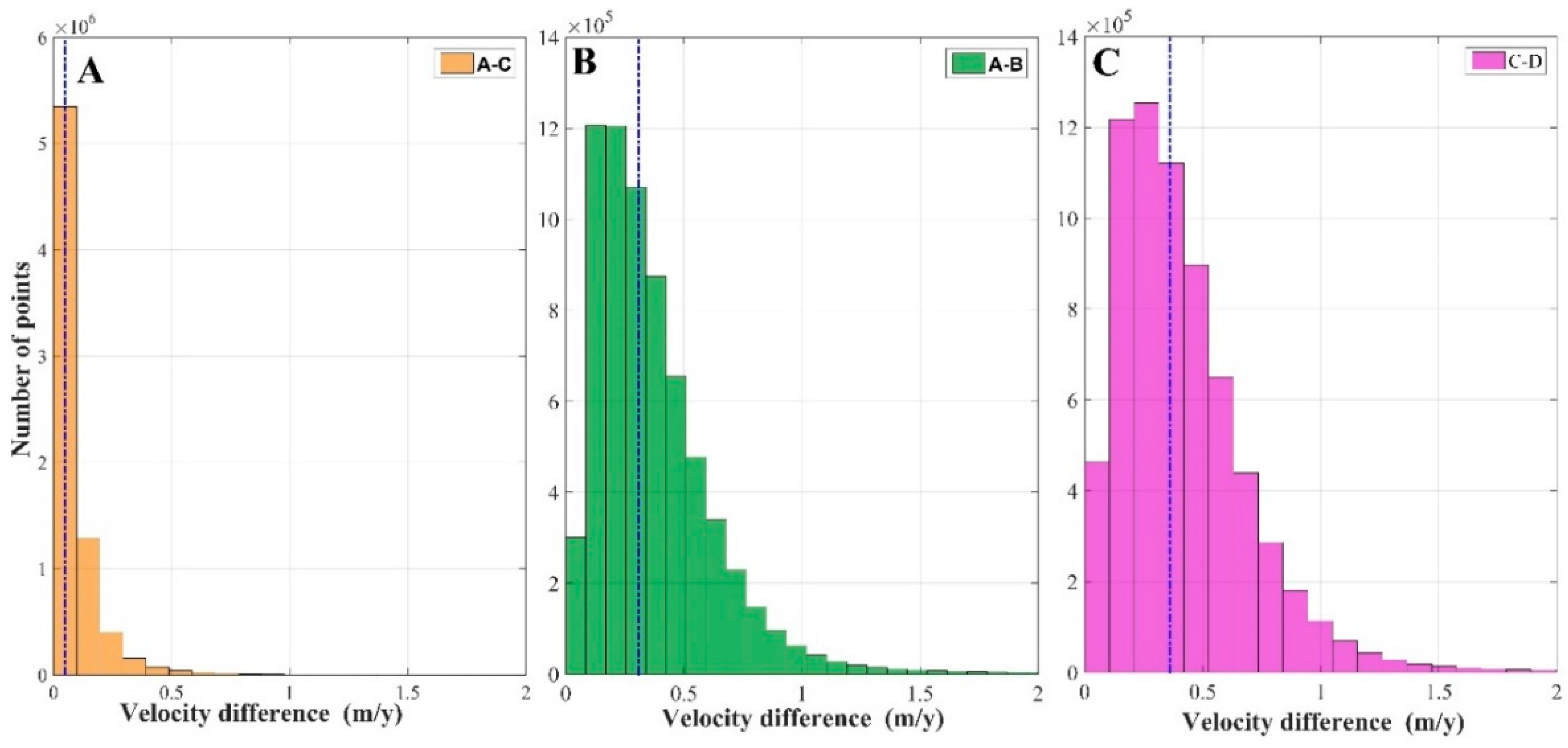
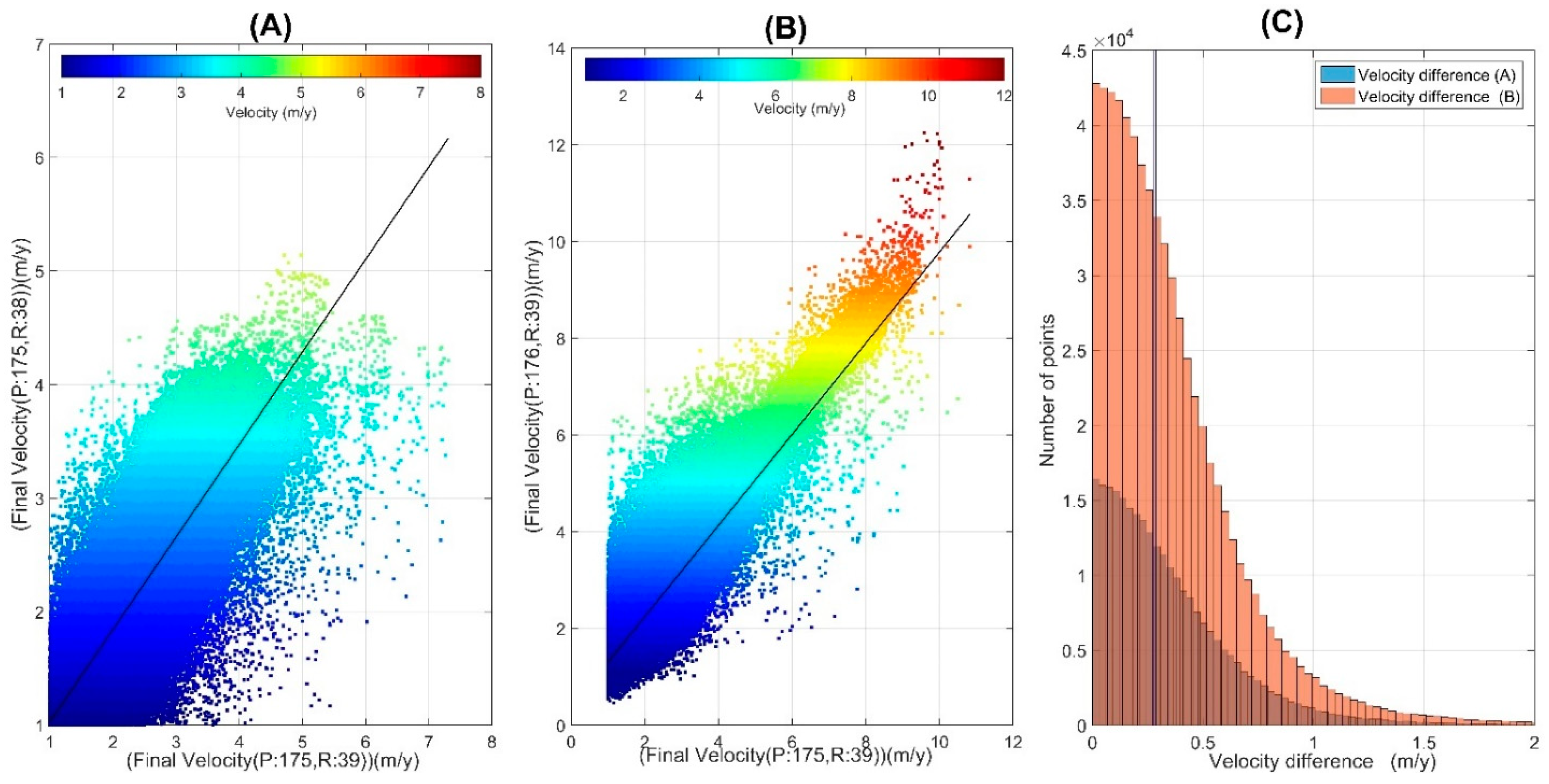
4.5. Cross Validation
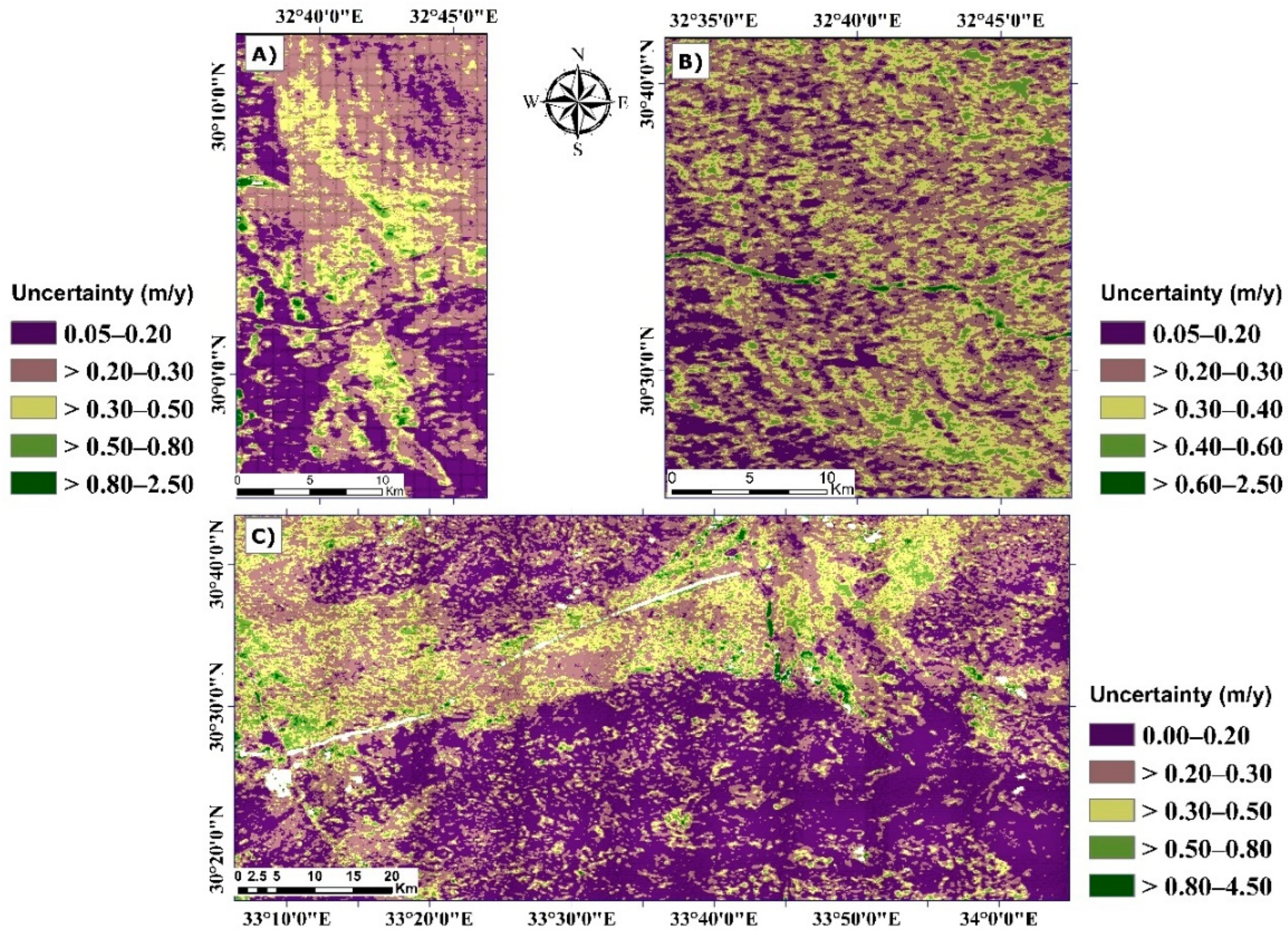
4.6. Uncertainty of Final Velocities
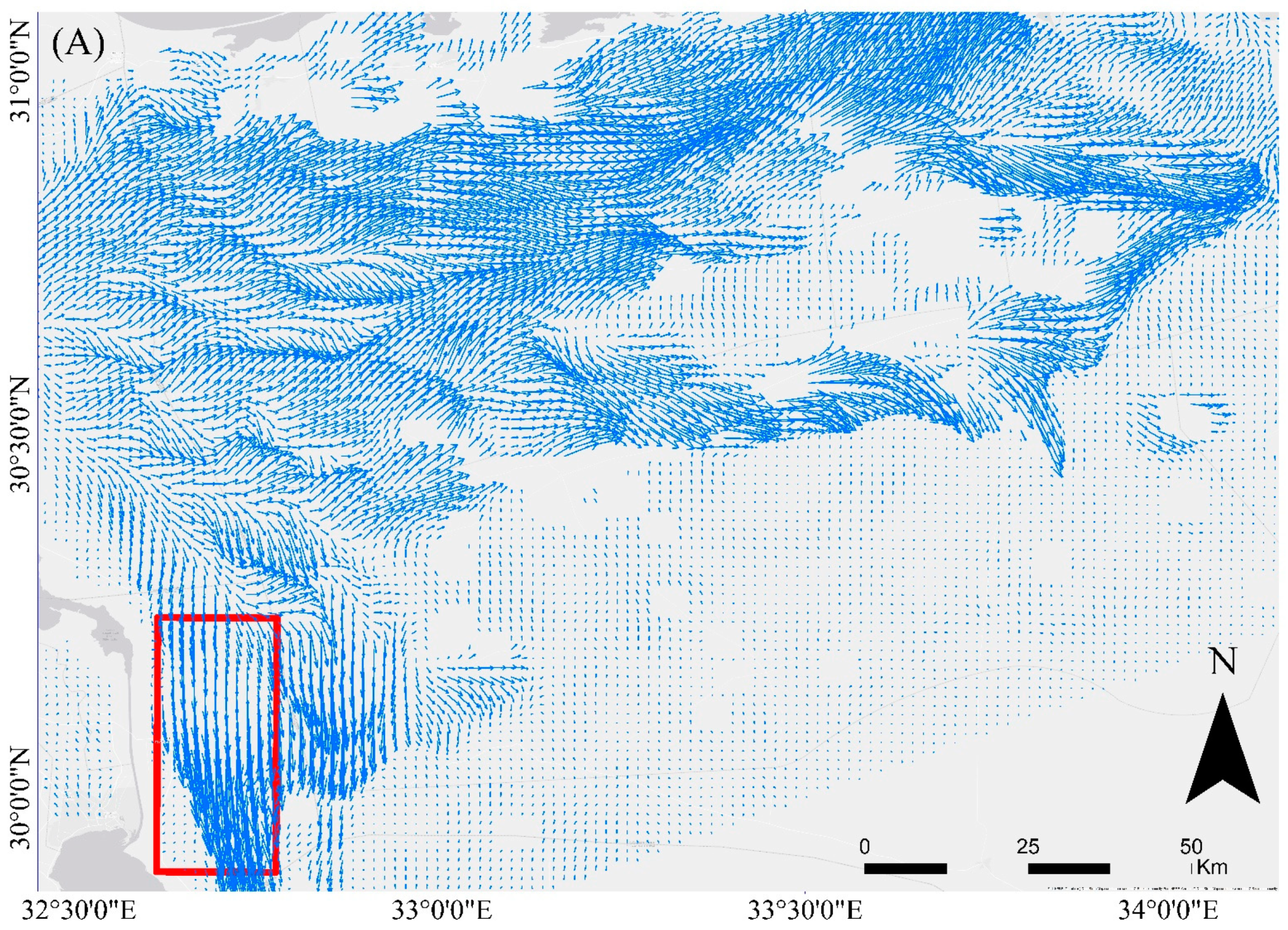
4.7. Analysis of Final Velocity Directions
5. Discussion
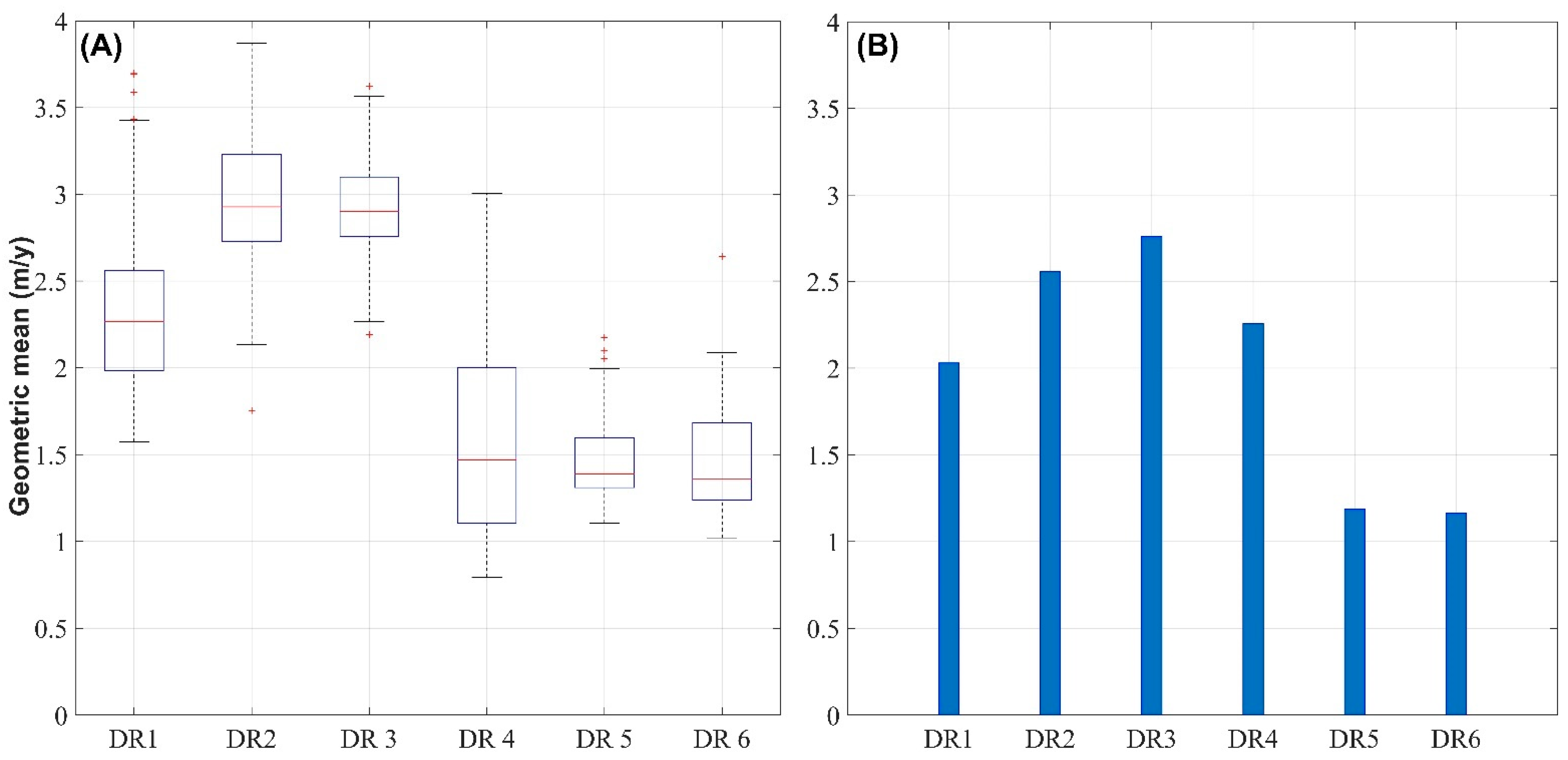
5.1. Spatiotemporal Variability of Dune Velocities
5.2. Comparison between the Combined Velocites and Individual Velocites
6. Conclusions
Supplementary Materials
Author Contributions
Funding
Institutional Review Board Statement
Informed Consent Statement
Acknowledgments
Conflicts of Interest
References
- Hugenholtz, C.H.; Levin, N.; Barchyn, T.E.; Baddock, M.C. Remote sensing and spatial analysis of aeolian sand dunes: A review and outlook. Earth Sci. Rev. 2012, 111, 319–334. [Google Scholar] [CrossRef]
- Scheidt, S.P.; Lancaster, N. The application of COSI-Corr to determine dune system dynamics in the southern Namib Desert using ASTER data. Earth Surf. Process. Landf. 2013, 38, 1004–1019. [Google Scholar] [CrossRef]
- Ashkenazy, Y.; Shilo, E. Sand dune Albedo feedback. Geosciences 2018, 8, 83. [Google Scholar] [CrossRef] [Green Version]
- Effat, H.; Hegazy, M.; Behr, F. Cartographic Modeling of Potential Sand Dunes Movement Risk Using Remote Sensing and Geographic Information System in Sinai, Egypt. In Landuse/Landcover of Sialkot Using RS & GIS—An Urban Sprawl Perspective; AGSE Publishing: Karlsruhe, Germany, 2012; pp. 139–148. [Google Scholar]
- Hamdan, M.A.; Refaat, A.A.; Abdel Wahed, M. Morphologic characteristics and migration rate assessment of barchan dunes in the Southeastern Western Desert of Egypt. Geomorphology 2016, 257, 57–74. [Google Scholar] [CrossRef]
- Ahmady-Birgani, H.; McQueen, K.G.; Moeinaddini, M.; Naseri, H. Sand Dune Encroachment and Desertification Processes of the Rigboland Sand Sea, Central Iran. Sci. Rep. 2017, 7, 1523. [Google Scholar] [CrossRef]
- Ding, C.; Zhang, L.; Liao, M.; Feng, G.; Dong, J.; Ao, M.; Yu, Y. Quantifying the spatio-temporal patterns of dune migration near Minqin Oasis in northwestern China with time series of Landsat-8 and Sentinel-2 observations. Remote Sens. Environ. 2020, 236, 111498. [Google Scholar] [CrossRef]
- Lam, D.K.; Remmel, T.K.; Drezner, T.D. Tracking desertification in California using remote sensing: A sand dune encroachment approach. Remote Sens. 2011, 3, 1–13. [Google Scholar] [CrossRef] [Green Version]
- Ding, C.; Feng, G.; Liao, M.; Zhang, L. Change detection, risk assessment and mass balance of mobile dune fields near Dunhuang Oasis with optical imagery and global terrain datasets. Int. J. Digit. Earth 2020, 13, 1604–1623. [Google Scholar] [CrossRef]
- Ghadiry, M.; Shalaby, A.; Koch, B. A new GIS-based model for automated extraction of Sand Dune encroachment case study: Dakhla Oases, western desert of Egypt. Egypt. J. Remote Sens. Sp. Sci. 2012, 15, 53–65. [Google Scholar] [CrossRef] [Green Version]
- Ali, M.; Latif, A.; Elhag, M.M. Combating Desertification in Sudan. In Environment and Ecology at the Beginning of 21st Century; St. Kliment Ohridski University Press: Sofia, Bulgaria, 2015; Chapter 18; pp. 256–266. [Google Scholar]
- Baird, T.; Bristow, C.; Vermeesch, P. Measuring Sand Dune Migration Rates with COSI-Corr and Landsat: Opportunities and Challenges. Remote Sens. 2019, 11, 2423. [Google Scholar] [CrossRef] [Green Version]
- Mohamed, I.N.L.; Verstraeten, G. Analyzing dune dynamics at the dune-field scale based on multi-temporal analysis of Landsat-TM images. Remote Sens. Environ. 2012, 119, 105–117. [Google Scholar] [CrossRef]
- Potter, C.; Weigand, J. Analysis of Desert Sand Dune Migration Patterns from Landsat Image Time Series for The Southern California Desert. J. Remote Sens. GIS 2016, 5, 1–8. [Google Scholar] [CrossRef] [Green Version]
- Levin, N.; Ben-Dor, E.; Karnieli, A. Topographic information of sand dunes as extracted from shading effects using Landsat images. Remote Sens. Environ. 2004, 90, 190–209. [Google Scholar] [CrossRef]
- Ali, E.; Xu, W. An optical image time series inversion method and application to long term sand dune movements in the Sinai Peninsula. In Proceedings of the European Geosciences Union (EGU), Vienna, Austria, 7–12 April 2019. [Google Scholar]
- Vermeesch, P.; Leprince, S. A 45-year time series of dune mobility indicating constant windiness over the central Sahara. Geophys. Res. Lett. 2012, 39. [Google Scholar] [CrossRef] [Green Version]
- Vermeesch, P.; Drake, N. Remotely sensed dune celerity and sand flux measurements of the world’s fastest barchans (Bodélé, Chad). Geophys. Res. Lett. 2008, 35, 1–6. [Google Scholar] [CrossRef] [Green Version]
- Necsoiu, M.; Leprince, S.; Hooper, D.M.; Dinwiddie, C.L.; McGinnis, R.N.; Walter, G.R. Monitoring migration rates of an active subarctic dune field using optical imagery. Remote Sens. Environ. 2009, 113, 2441–2447. [Google Scholar] [CrossRef]
- Hermas, E.S.; Alharbi, O.; Alqurashi, A.; Niang, A.J.; Al-Ghamdi, K.; Al-Mutiry, M.; Farghaly, A. Characterisation of sand accumulations in Wadi Fatmah and Wadi Ash Shumaysi, KSA, Using multi-source remote sensing imagery. Remote Sens. 2019, 11, 2824. [Google Scholar] [CrossRef] [Green Version]
- Hermas, E.; Leprince, S.; El-Magd, I.A. Retrieving sand dune movements using sub-pixel correlation of multi-temporal optical remote sensing imagery, northwest Sinai Peninsula, Egypt. Remote Sens. Environ. 2012, 121, 51–60. [Google Scholar] [CrossRef]
- Al-Ghamdi, K.; Hermas, E. Assessment of dune migration hazards against landuse northwest Al-lith City, Saudi Arabia, using multi-temporal satellite imagery. Arab. J. Geosci. 2015, 8, 11007–11018. [Google Scholar] [CrossRef]
- Al-Mutiry, M.; Hermas, E.A.; Al-Ghamdi, K.A.; Al-Awaji, H. Estimation of dune migration rates north Riyadh City, KSA, using SPOT 4 panchromatic images. J. Afr. Earth Sci. 2016, 124, 258–269. [Google Scholar] [CrossRef]
- Els, A.; Merlo, S.; Knight, J. Comparison of two Satellite Imaging Platforms for Evaluating Sand Dune Migration in the Ubari Sand Sea (Libyan Fazzan). Int. Arch. Photogramm. Remote. Sens. Spat. Inf. Sci. 2015, 40, 1375–1380. [Google Scholar] [CrossRef] [Green Version]
- Ali, E.; Xu, W.; Ding, X. Improved optical image matching time series inversion approach for monitoring dune migration in North Sinai Sand Sea: Algorithm procedure, application, and validation. ISPRS J. Photogramm. Remote Sens. 2020, 164, 106–124. [Google Scholar] [CrossRef]
- Dong, P. Automated measurement of sand dune migration using multi-temporal lidar data and GIS. Int. J. Remote Sens. 2015, 36, 5426–5447. [Google Scholar] [CrossRef]
- Dong, P.; Xia, J.; Zhong, R.; Zhao, Z.; Tan, S. A New Method for Automated Measurement of Sand Dune Migration Based on Multi-Temporal LiDAR-Derived Digital Elevation Models. Remote Sens. 2021, 13, 3084. [Google Scholar] [CrossRef]
- Grohmann, C.H.; Garcia, G.P.B.; Affonso, A.A.; Albuquerque, R.W. Dune migration and volume change from airborne LiDAR, terrestrial LiDAR and Structure from Motion-Multi View Stereo. Comput. Geosci. 2020, 143, 104569. [Google Scholar] [CrossRef]
- Pagán, J.I.; Bañón, L.; López, I.; Bañón, C.; Aragonés, L. Monitoring the dune-beach system of Guardamar del Segura (Spain) using UAV, SfM and GIS techniques. Sci. Total Environ. 2019, 687, 1034–1045. [Google Scholar] [CrossRef]
- Laporte-Fauret, Q.; Marieu, V.; Castelle, B.; Michalet, R.; Bujan, S.; Rosebery, D. Low-Cost UAV for high-resolution and large-scale coastal dune change monitoring using photogrammetry. J. Mar. Sci. Eng. 2019, 7, 63. [Google Scholar] [CrossRef] [Green Version]
- Leprince, S.; Barbot, S.; Ayoub, F.; Avouac, J.-P. Automatic and Precise Orthorectification, Coregistration, and Subpixel Correlation of Satellite Images, Application to Ground Deformation Measurements. IEEE Geosci. Remote Sens. Lett. 2007, 45, 1529–1558. [Google Scholar] [CrossRef] [Green Version]
- Sam, L.; Gahlot, N.; Prusty, B.G. Estimation of dune celerity and sand flux in part of West Rajasthan, Gadra area of the Thar Desert using temporal remote sensing data. Arab. J. Geosci. 2015, 8, 295–306. [Google Scholar] [CrossRef]
- Bridges, N.T.; Ayoub, F.; Avouac, J.; Leprince, S.; Lucas, A.; Mattson, S. Earth-like sand fluxes on Mars. Nature 2012, 485, 339–342. [Google Scholar] [CrossRef] [PubMed] [Green Version]
- Ayoub, F.; Avouac, J.-P.; Newman, C.E.; Richardson, M.I.; Lucas, A.; Leprince, S.; Bridges, N.T. Threshold for sand mobility on Mars calibrated from seasonal variations of sand flux. Nat. Commun. 2014, 5, 5096. [Google Scholar] [CrossRef] [Green Version]
- Davis, J.M.; Grindrod, P.M.; Boazman, S.J.; Vermeesch, P.; Baird, T. Quantified Aeolian Dune Changes on Mars Derived From Repeat Context Camera Images. Earth Sp. Sci. 2020, 7, e2019EA000874. [Google Scholar] [CrossRef] [Green Version]
- Kääb, A.; Winsvold, S.; Altena, B.; Nuth, C.; Nagler, T.; Wuite, J. Glacier Remote Sensing Using Sentinel-2. Part I: Radiometric and Geometric Performance, and Application to Ice Velocity. Remote Sens. 2016, 8, 598. [Google Scholar] [CrossRef] [Green Version]
- Fahnestock, M.; Scambos, T.; Moon, T.; Gardner, A.; Haran, T.; Klinger, M. Rapid large-area mapping of ice flow using Landsat 8. Remote Sens. Environ. 2016, 185, 84–94. [Google Scholar] [CrossRef] [Green Version]
- Bontemps, N.; Lacroix, P.; Doin, M. Inversion of deformation fields time-series from optical images, and application to the long term kinematics of slow-moving landslides in Peru. Remote Sens. Environ. 2018, 210, 144–158. [Google Scholar] [CrossRef]
- Ding, C.; Feng, G.; Li, Z.; Shan, X.; Du, Y.; Wang, H. Spatio-Temporal Error Sources Analysis and Accuracy Improvement in Landsat 8 Image Ground Displacement Measurements. Remote Sens. 2016, 8, 937. [Google Scholar] [CrossRef] [Green Version]
- Leprince, S.; Member, S.; Musé, P.; Avouac, J. In-Flight CCD Distortion Calibration for Pushbroom Satellites Based on Subpixel Correlation. IEEE Geosci. Remote Sens. Lett. 2008, 46, 2675–2683. [Google Scholar] [CrossRef]
- Lacroix, P.; Bièvre, G.; Pathier, E.; Kniess, U.; Jongmans, D. Use of Sentinel-2 images for the detection of precursory motions before landslide failures. Remote Sens. Environ. 2018, 215, 507–516. [Google Scholar] [CrossRef]
- Dehecq, A.; Gourmelen, N.; Trouve, E. Deriving large-scale glacier velocities from a complete satellite archive: Application to the Pamir–Karakoram–Himalaya. Remote Sens. Environ. 2015, 162, 55–66. [Google Scholar] [CrossRef] [Green Version]
- Mouginot, J.; Rignot, E.; Scheuchl, B.; Millan, R. Comprehensive annual ice sheet velocity mapping using Landsat-8, Sentinel-1, and RADARSAT-2 data. Remote Sens. 2017, 9, 364. [Google Scholar] [CrossRef] [Green Version]
- Millan, R.; Mouginot, J.; Rabatel, A.; Jeong, S.; Cusicanqui, D.; Derkacheva, A.; Chekki, M. Mapping surface flow velocity of glaciers at regional scale using a multiple sensors approach. Remote Sens. 2019, 11, 2498. [Google Scholar] [CrossRef] [Green Version]
- Derkacheva, A.; Mouginot, J.; Millan, R.; Maier, N.; Gillet-Chaulet, F. Data reduction using statistical and regression approaches for ice velocity derived by Landsat-8, Sentinel-1 and Sentinel-2. Remote Sens. 2020, 12, 1935. [Google Scholar] [CrossRef]
- Bubenzer, O.; Embabi, N.S.; Ashour, M.M. Sand seas and dune fields of Egypt. Geosciences 2020, 10, 101. [Google Scholar] [CrossRef] [Green Version]
- Embabi, N.S. Landscapes and Landforms of Egypt: World Geomorphological Landscapes; Springer: Berlin/Heidelberg, Germany, 2018; ISBN 978-3-319-65659-5. [Google Scholar]
- ElBanna, M.S. Geological Studies Emphasizing the Morphology and Dynamics of Sand Dunes and their Environmental Impacts on the Reclamation and Developmental Areas in Northwest Sinai, Egypt. Ph.D. Thesis, Cairo University, Cairo, Egypt, 2004. [Google Scholar]
- Scherler, D.; Leprince, S.; Strecker, M.R. Glacier-surface velocities in alpine terrain from optical satellite imagery—Accuracy improvement and quality assessment. Remote Sens. Environ. 2008, 112, 3806–3819. [Google Scholar] [CrossRef]
- Paul, F.; Bolch, T.; Briggs, K.; Kääb, A.; McMillan, M.; McNabb, R.; Nagler, T.; Nuth, C.; Rastner, P.; Strozzi, T.; et al. Error sources and guidelines for quality assessment of glacier area, elevation change, and velocity products derived from satellite data in the Glaciers_cci project. Remote Sens. Environ. 2017, 203, 256–275. [Google Scholar] [CrossRef] [Green Version]
- Shukla, A.; Garg, P.K. Spatio-temporal trends in the surface ice velocities of the central Himalayan glaciers, India. Glob. Planet. Chang. 2020, 190, 103187. [Google Scholar] [CrossRef]
- Stumpf, A.; Malet, J.P.; Delacourt, C. Correlation of satellite image time-series for the detection and monitoring of slow-moving landslides. Remote Sens. Environ. 2017, 189, 40–55. [Google Scholar] [CrossRef]
- Fryberger, S.G. Mechanisms for the formation of eolian sand seas. Zeitschrift für Geomorphol. Ann. Geomorphol. Ann. Géomorphologie 1979, 23, 440–460. [Google Scholar]


| Sensor | Frame (Path/Row) | Pairs/Images | Observation Period | Baselines | |||
|---|---|---|---|---|---|---|---|
| SED (°) | SAD (°) | TS (Yr.) | SB (m) | ||||
| L8 | 176/39 | 113/52 | 4/9/2013–3/26/2018 | 10 | 10 | 1–4 | 250 |
| 175/39 | 46/30 | 7/11/2013–6/7/2018 | |||||
| 175/38 | 31/33 | 6/25/2013–3/3/2018 | |||||
| 174/39 | 70/46 | 5/1/2013–4/13/2018 | |||||
| S2 | TR36VU | 51/30 | 12/21/2015–2/13/2019 | 9 | 9 | 1–3 | -- |
| T36RXV | 53/40 | 20/8/2015–22/12/2018 | |||||
| Pair ID | Master | Slave | TS (Days) | MAD of Stable Targets (m/y) |
|---|---|---|---|---|
| 1 | 2/11/2014 | 3/15/2014 | 32 | 4.44 |
| 2 | 3/31/2014 | 48 | 3.74 | |
| 3 | 4/16/2014 | 64 | 3.42 | |
| 4 | 5/18/2014 | 96 | 3.61 | |
| 5 | 3/2/2015 | 384 | 0.32 | |
| 6 | 3/4/2016 | 752 | 0.20 | |
| 7 | 10/14/2016 | 976 | 0.18 | |
| 8 | 12/17/2016 | 1040 | 0.18 | |
| 9 | 2/3/2017 | 1088 | 0.13 | |
| 10 | 2/22/2018 | 1472 | 0.10 |
| Component | r | ||
|---|---|---|---|
| EW | 3.10 | 0.56 | 0.99 |
| NS | 2.40 | 0.47 | 0.97 |
Publisher’s Note: MDPI stays neutral with regard to jurisdictional claims in published maps and institutional affiliations. |
© 2021 by the authors. Licensee MDPI, Basel, Switzerland. This article is an open access article distributed under the terms and conditions of the Creative Commons Attribution (CC BY) license (https://creativecommons.org/licenses/by/4.0/).
Share and Cite
Ali, E.; Xu, W.; Ding, X. Spatiotemporal Variability of Dune Velocities and Corresponding Uncertainties, Detected from Optical Image Matching in the North Sinai Sand Sea, Egypt. Remote Sens. 2021, 13, 3694. https://doi.org/10.3390/rs13183694
Ali E, Xu W, Ding X. Spatiotemporal Variability of Dune Velocities and Corresponding Uncertainties, Detected from Optical Image Matching in the North Sinai Sand Sea, Egypt. Remote Sensing. 2021; 13(18):3694. https://doi.org/10.3390/rs13183694
Chicago/Turabian StyleAli, Eslam, Wenbin Xu, and Xiaoli Ding. 2021. "Spatiotemporal Variability of Dune Velocities and Corresponding Uncertainties, Detected from Optical Image Matching in the North Sinai Sand Sea, Egypt" Remote Sensing 13, no. 18: 3694. https://doi.org/10.3390/rs13183694
APA StyleAli, E., Xu, W., & Ding, X. (2021). Spatiotemporal Variability of Dune Velocities and Corresponding Uncertainties, Detected from Optical Image Matching in the North Sinai Sand Sea, Egypt. Remote Sensing, 13(18), 3694. https://doi.org/10.3390/rs13183694