Retrieval of Daily Mean Top-of-Atmosphere Reflected Solar Flux Using the Advanced Very High Resolution Radiometer (AVHRR) Instruments

Abstract

The records of the Advanced Very High Resolution Radiometer (AVHRR) instrument observations can resolve the current lack of a long global climate data record of Reflected Solar Flux (RSF), by transforming these measurements into broadband flux at the top-of-atmosphere. This paper presents a methodology for obtaining daily mean RSF (Wm${}^{-2}$) from AVHRR. First, the narrowband reflectances are converted to broadband reflectance using empirical regressions with the Clouds and the Earth’s Radiant Energy System (CERES) observations. Second, the anisotropy is corrected by applying Angular Distribution Models (ADMs), which convert directional reflectance into a hemispherical albedo. Third, the instantaneous albedos are temporally interpolated by a flexible diurnal cycle model, capable of ingesting any number of observations at any time of day, making it suitable for any orbital configuration of NOAA and MetOp satellites. Finally, the twilight conditions prevailing near sunrise and sunset are simulated with an empirical model. The entire day is then integrated into a single daily mean RSF. This paper furthermore demonstrates the methodology by validating a full year (2008) of RSF daily means with the CERES SYN1deg data record, both on daily and subdaily scale. Several configurations are tested, each excluding particular satellites from the constellation in order to mimic orbital changes (e.g., orbital drift), and to assess their relative importance to the daily mean RSF. The best performance is obtained by the combination of at least one mid-morning (NOAA-17 or MetOp-A) and one early afternoon (NOAA-18) orbit. In this case, the RMS difference with CERES is about 7 Wm${}^{-2}$. Removing NOAA-18 degrades the performance to an RMS difference of 12 Wm${}^{-2}$, thereby providing an estimate of the impact of NOAA-19’s orbital drift between 2016 and 2020. Very early or late observations (NOAA-15, NOAA-16) provide little added value, and both mid-morning orbits turn out to be almost interchangeable given their close temporal proximity.

1. Introduction

Broadband top-of-atmosphere (TOA) Reflected Solar Flux (RSF) is an essential climate variable of which a high-quality data record of satellite measurements with sufficient length (“Climate Data Record” or CDR) is needed by, among others, the climate modeling and climate monitoring communities, preferably spanning several decades [1].

To this end, various approaches have been proposed and implemented (a review is available in Dewitte and Clerbaux [2]). In the Earth Radiation Budget Experiment (ERBE) [3], narrow- and wide-Field-Of-View (FOV) radiometers have been deployed. In recent Earth Radiation Budget (ERB) missions, such as the Clouds and Earth’s Radiant Energy System (CERES) [4], the Geostationary Earth Radiation Budget (GERB) [5] or the Scanner for Radiation Budget (ScaRaB) [6], the narrow-FOV approach has been selected because the wide-FOV provided limited scientific outcomes due to the enormous size of the FOV and the difficulty of relating the fluxes with particular scene types. All these dedicated ERB missions rely on broadband (BB) radiometers that provide integrated observations of the radiation over large parts of the electromagnetic spectrum: “shortwave” (0.3–4$\mathsf{\mu }\mathrm{m}$) and “longwave” (4–50$\mathsf{\mu }\mathrm{m}$). Such instruments are not widely deployed in space because the usefulness of their data is mostly limited to the particular ERB community. This is in contrast to other multi-spectral instruments, such as MODIS, which are useful for a wide range of different geophysical variables.

In parallel to BB radiometers, several projects have provided useful ERB records that are not based on BB observations but on either atmospheric reanalysis, for example, ERA5 [7,8], or on cloud observations complemented by radiative transfer models (RTMs). The latter is the case with the well known ISCCP-FH dataset [9] and with the recent TOA fluxes produced by the ESA Cloud_cci project [10,11]. This approach has the advantage of simultaneously providing the all-sky and clear-sky TOA fluxes, allowing a direct estimation of the cloud radiative effect. Another advantage is that it can be applied to visible (and infrared) imagery of historical weather satellites that have been primarily designed for cloud observations (e.g., as in ISCCP). However, radiative transfer computations are more subject to biases due to the necessarily simplified description of optical properties of the surface, atmosphere, aerosols and cloudiness.

As a third approach, TOA fluxes have been also estimated from visible (and infrared) observations from weather satellites using a so-called narrowband-to-broadband conversion, to estimate broadband radiation from one or several observations taken at different wavelengths in the spectrum. The conversion can itself be based on radiative transfer simulation (“theoretical” approach) or based on collocated observations with a broadband instrument (“empirical” approach). An example for longwave radiation is the widely used data record of HIRS OLR [12]. Urbain et al. [13] show how shortwave narrowband-to-broadband conversions have been used to derive a long dataset of TOA RSF using the visible channels of the Meteosat satellites (1983–2015); however, products based on geostationary satellites do not provide global coverage.

Among those approaches and products, the global CERES products (first approach) are acknowledged to be the golden standard with respect to radiative flux data records, although two limitations can be identified: (1) the records are relatively recent, for example, starting in the year 2000 for the EBAF product; and (2) the products have a relatively coarse spatial resolution of 1${}^{\circ }$ (lat-lon equal angle grid), cf. Figure 1a.

To date, no harmonized global CDR of TOA RSF dating back to the 1970s or 1980s exists. Based on the above mentioned third approach, an alternative method is to rely on existing global long-term CDRs of harmonized narrowband reflectance (FDRs), for example, from the Advanced Very High Resolution Radiometer (AVHRR) instrument [14,15], and to transform these measurements into broadband quantities [16]. A preceding paper documents the retrieval of instantaneous broadband reflectance from the narrowband AVHRR observations [17] by establishing robust relations between the narrowband AVHRR measurements and the broadband measurements from CERES.

Using this AVHRR-derived broadband reflectance, the current paper describes the retrieval of the daily mean RSF (Wm${}^{-2}$), which could then be aggregated to monthly means to constitute a long-term, broadband energy balance dataset that would fit the needs of the climate modeling and monitoring communities. This is done on a global grid with a spatial resolution of 0.25${}^{\circ }$ (Figure 1b). The methods and algorithms described in this article are used for the upcoming third edition of the CM SAF Cloud, Albedo And Surface Radiation dataset from 42 years of AVHRR data, 3rd edition (CLARA-A3). The first and second editions are described by [18,19], respectively, and do not yet include TOA radiative fluxes.

In addition to the Reflected Solar Flux, the algorithm also estimates the TOA incoming solar radiation (based on daily TSI and Earth orbit parameters). The third component of the Earth radiation budget, the Outgoing Longwave Radiation, is described in Clerbaux et al. [20].

The AVHRR observation density on a given day is not constant. It varies over time, depending on the number of AVHRR-carrying satellites at any particular moment (Figure 2a). It also varies in space because the polar orbit causes the consecutive swaths to overlap towards the poles, thereby increasing the number of observations on a given location (Figure 2b). This requires a flexible algorithm capable of ingesting any number of observations.

The daily mean RSF is derived by integrating daytime, twilight, and nighttime fluxes. Twilight RSF is estimated by applying an empirical model. Daytime RSF is estimated by applying an interpolation method that seamlessly fuses observations with an empirical diurnal cycle model, which requires at least one (daytime) observation per 24 h; higher accuracy, however, is obtained with higher observation density (Figure 2).

Section 2 provides an overview of the input data necessary for the TOA flux retrieval. Subsequently, Section 3 describes the methodological framework of the TOA flux retrieval. Finally, Section 4 validates the method by comparing the obtained RSF with the state-of-the-art products, CERES SYN1deg-Day and SYN1deg-Hour, Ed4.1.

2. Input Data

The selection of all input data described below is based on the requirement of continuous spatial (global) and temporal (1979–2020) coverage. The overview of the input data given here is rather concise, and a more detailed documentation [21] provides additional clarifications on their implementation, technical details, and example figures.

2.1. External Input Data

Table 1. External input data: overview.

Data Type	Data Source	Data Accessibility
FDR AVHRR radiances ${\rho }_{0.6},{\rho }_{0.8}$	EUMETSAT *	PPS (v2018-patch5) L1c output
Cloud products	CMSAF CLARA-A3	PPS (v2018-patch5) L2 output
Snow depth	ERA5 reanalysis [7]	C3S Climate Data Store **
Wind speed	ERA5 reanalysis [7]	C3S Climate Data Store **
Sea ice conc.	OSI SAF [30]	Archive HL FTP server **
TSI	C3S/RMIB [2,31]	C3S Climate Data Store
COT climatology	CERES EBAF [32]	https://ceres.larc.nasa.gov/ (accessed on 1 August 2021)
Land cover map (30” res.)	IGBP classification applied	USGS Earth Explorer
	on GLCC database [33,34]
Land cover map (10’ res.)	CERES surface type map	pers.comm. N.Loeb [21]
ADMs	CERES [35,36]	https://ceres.larc.nasa.gov/ (accessed on 1 August 2021)

* Processed by EUMETSAT using the CMSAF PyGAC tool [22]. ** These variables are in theory accessible on those locations, but were in practice regridded to the orbit grid and made available to the authors in that format (together with the PPS output).

provides an overview of the external input data, that is, data not generated by the authors. From AVHRR Global Area Coverage (GAC) Level-1c data, a Fundamental Data Record (FDR) is created using the PyGAC processor tool [22], performing the calibration and homogenization of the record. It is a Python package to read, calibrate and navigate NOAA and MetOp AVHRR data. Scaled radiance ($S{R}_{\lambda }$) from shortwave channels 1 + 2, on 0.6$\mathsf{\mu }\mathrm{m}$ and 0.8$\mathsf{\mu }\mathrm{m}$, are provided on their original irregular GAC orbit grid together with the necessary metadata. The time stamp, geolocation, and viewing and illumination geometry (solar zenith angle ${\theta }_0$, viewing zenith angle $\theta$, relative azimuth angle $\varphi$) are also included. Channel 1 and channel 2 scaled radiances are already normalized to account for the seasonally changing Earth–Sun distance.

The NWC SAF Polar Platform System (PPS) consists of a cloud processing software package for polar orbiting satellite data provided by the EUMETSAT NWC SAF project [23,24]. It includes the Cloud Physical Properties (CPP) algorithm [25], which retrieves the cloud thermodynamic phase, cloud optical thickness (COT), cloud particle effective radius, and liquid/ice water path. The products used in this article are based on version PPSv2018-patch5, which will also be implemented in the CLARA-A3 products. The following PPS products are used for the TOA flux retrieval: PPS probabilistic cloud mask [26,27], PPS classic cloud mask with snow presence flag [19,28], and PPS-CPP cloud phase, optical thickness, and quality flag [29].

The remaining input data consist of ERA5 reanalysis of snow depth and wind speed [7], OSI SAF sea ice concentration from products OSI-450 and OSI-430-b [30], daily Total Solar Irradiance (TSI) from the Copernicus Climate Change Service (C3S) based on Dewitte and Nevens [31] and Dewitte and Clerbaux [2], and an average annual cycle (climatology) of COT calculated from CERES EBAF Ed.4.1 [21,32]. Static input data consist of a 30 arc-second GLCC land cover map using IGBP classification [33,34], and a CERES low-resolution (10’) land cover map [21].

Finally, important static input data include the CERES shortwave Angular Distribution Models (ADMs). The models consist of radiance measurements stratified by discretized angular bins describing viewing and illumination geometry (${\theta }_0$, $\theta$, $\varphi$) resulting in three-dimensional data structures. For each solar zenith angle bin, the ADMs also provide the hemispherically integrated radiance, that is, Flux, which is also provided in terms of albedo (so-called ${\theta }_0$-dependent “albedo model”). Together these data make up the ADM, which describes the radiance’s anisotropy. Models are constructed for a variety of land surface types and cloud properties, together constituting so-called “scene types”. The TRMM Shortwave Ed.2B ADMs [35] are derived from 8 months of observations from the CERES instrument in Rotating Azimuth Plane Scan (RAPS) mode on board the Tropical Rainfall Measurement Mission (TRMM) satellite. Since this satellite was flying on a sun precessing orbit, these ADM models span the entire ${\theta }_0$ range, which makes it well suited to generating ADMs. On the other hand, as the inclination of the TRMM orbit was only 35${}^{\circ }$ above the equatorial plane, the mid- and high-latitude regions have not been sampled, which means that snow and ice are not taken into account: for these scene types, the Terra Shortwave Ed.2B ADMs [36] are used, derived from the polar-orbiting Terra satellite.

2.2. Twilight Model and Coefficients

The RSF during twilight conditions is derived with an empirical model in which it linearly depends on the solar zenith angle (${\theta }_0$). A regression model (Equation (1)) mimics the average flux-${\theta }_0$ relation in the instantaneous CERES Single Scanner Footprint (SSF) TOA shortwave fluxes (in Wm${}^{-2}$), with ${\theta }_0$ ranging between 84–86.5${}^{\circ }$ for (parts of) years 2004, 2005, 2007, 2008, 2011, 2012. The regression model is written as follows:

$$F_{twilight}=A+({\theta }_0-{84}^{\circ })·B,$$

(1)

where $F_{twilight}$ stands for Flux during twilight conditions (Wm${}^{-2}$), A and B are the twilight coefficients, and ${\theta }_0$ is the Solar Zenith Angle (degrees). The models are created for five different Twilight (TWL) surface types separately for clear-sky and overcast conditions. Clear-sky is defined as an SSF footprint with 0% cloud cover and overcast as 100% cloud cover. The sample size (n) for each scene type is given in

Table 2. Twilight model: sample size (n) and regression coefficients (A, B).

Cloud Class	Clear-Sky			Overcast
TWL Surface Type	$\mathit{n}$	$\mathbf{A}\left[{\mathbf{Wm}}^{-2}\right]$	$\mathbf{B}\left[{\mathbf{Wm}}^{-2}{/}^{\circ }\right]$	$\mathit{n}$	$\mathbf{A}\left[{\mathbf{Wm}}^{-2}\right]$	$\mathbf{B}\left[{\mathbf{Wm}}^{-2}{/}^{\circ }\right]$
Water	34,283	41.749	−5.114	4,969,304	83.833	−12.835
Sea ice 100%	141,835	83.897	−12.784	375,797	92.968	−13.628
Perm.snow/ice	1,626,464	96.117	−14.699	1,879,264	99.274	−15.704
Fresh snow	86,142	60.456	−8.476	652,909	90.565	−13.671
Land	7902	38.724	−5.501	102,852	85.617	−12.739

.

The models are shown in Figure 3 for clear-sky conditions (left) and overcast conditions (right): the solid lines represent the observations as ${\theta }_0$ bin averages, demonstrating the linear nature of the flux-${\theta }_0$ relation, and its scene type dependency. From these observations, linear regressions were derived to extrapolate the flux for ${\theta }_0$ higher than 86.5${}^{\circ }$ (dotted lines). The intercept (A) and slope (B) of these regressions are listed in Table 2.

2.3. Narrowband-to-Broadband Coefficients

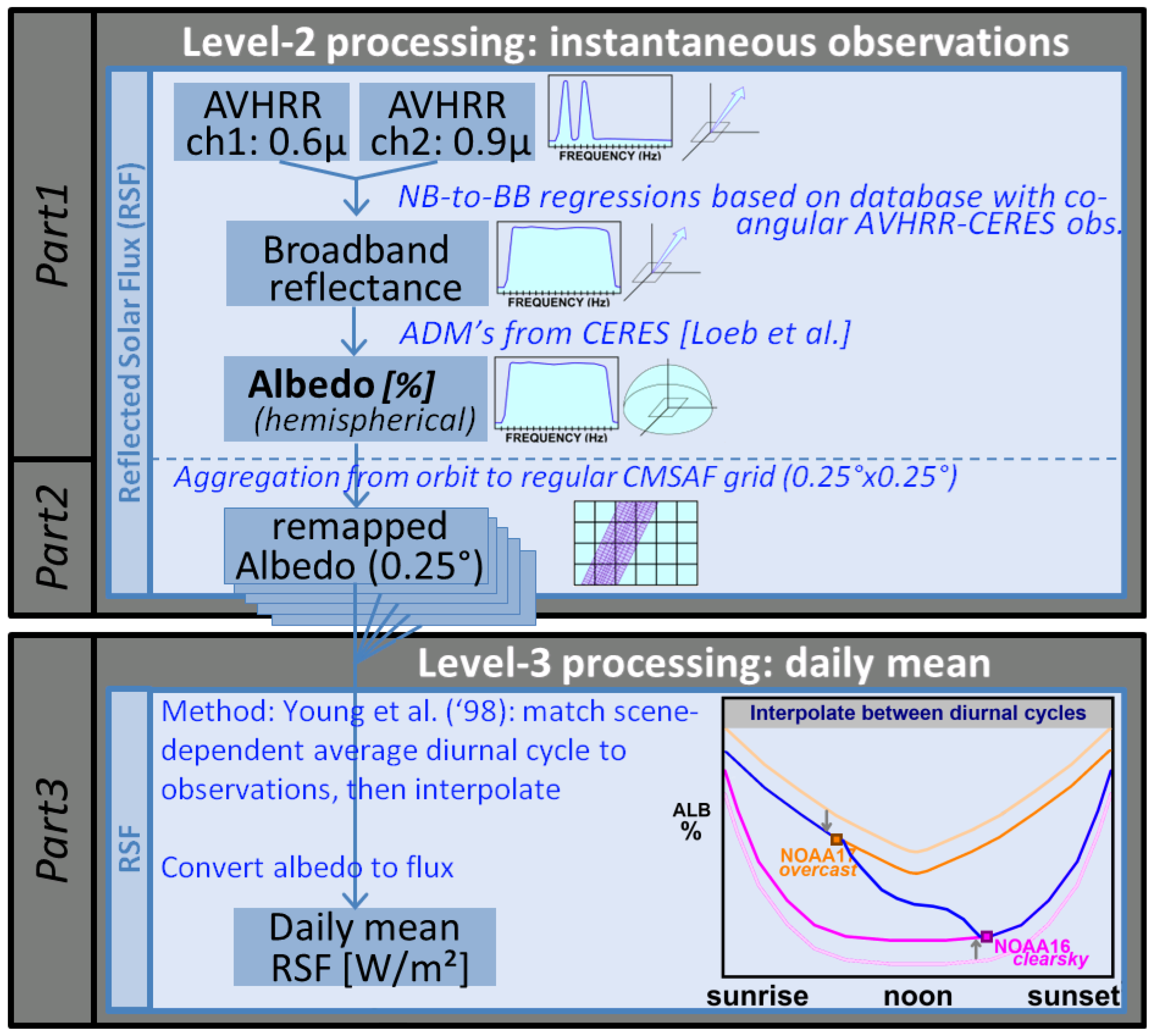
Conversion of narrowband to broadband (NTB) reflectance was carried out empirically by creating multivariate linear regressions on matched AVHRR-CERES observations (i.e., collocated, coangular, and simultaneous). The method is explained in detail by Akkermans and Clerbaux [17]. Achieving a sufficient matching sample size is only possible when the orbital planes of both CERES- and AVHRR-carrying satellites coincide, which limits the amount of useful data to these favorable periods (2004–2005, 2007–2008, 2011–2012). The spatial resolution of AVHRR and CERES is at nadir at about 4 km and 32 km, respectively, which requires a considerable spatial aggregation of AVHRR footprints to match a single CERES footprint. The main objective of Akkermans and Clerbaux (2020) was to derive regressions with high scene-specific accuracy, which is possible by narrowing down each scene type to a very homogeneous sample. However, there is a trade-off between the regression-specific theoretical accuracy (=internal), and the practical accuracy of the regressions when applied to the entire range of possible scene types (global result), including non-homogeneous scenes. Therefore, it was decided to slightly modify the regressions from Akkermans and Clerbaux [17] by loosening the cloud cover range, thereby redefining the “clear-sky” and “overcast” regressions: (1) “clear-sky” is now defined as cloud cover from 0% to 10% (instead of strictly 0%), and (2) “overcast” is now defined as cloud cover from 90% to 100% (instead of strictly 100%). Note that the cloud cover thresholds are imposed on both (fractional) AVHRR and CERES cloud masks in the SSF footprint, for example, clear-sky means that both cloud fractions should be below 10%. Furthermore, some small bug fixes in the code were found and solved. Together, the above mentioned adaptations resulted in updated coefficients, listed in

Table 3. NTB (Narrowband-to-Broadband) regression coefficients to be used in Equation (3), generated from all matched NTB pairs (update of Table 3 in Akkermans and Clerbaux [17]).

	Clear-Sky					Overcast
NTB Surface Type	${\mathit{b}}_{\mathbf{0}}$	${\mathit{b}}_{\mathbf{1}}$	${\mathit{b}}_{\mathbf{2}}$	${\mathit{b}}_{\mathbf{3}}$	${\mathit{b}}_{\mathbf{4}}$	${\mathit{b}}_{\mathbf{0}}$	${\mathit{b}}_{\mathbf{1}}$	${\mathit{b}}_{\mathbf{2}}$	${\mathit{b}}_{\mathbf{3}}$	${\mathit{b}}_{\mathbf{4}}$
Ocean	1.811	1.148	−0.523	−0.043	0.390	4.013	0.313	0.447	0.709	1.286
Forests	1.471	0.480	0.377	1.358	1.211	3.622	0.366	0.395	0.905	1.542
Savannas	1.421	0.463	0.382	2.696	0.769	3.328	0.403	0.355	4.127	1.059
Grass/crop	2.575	0.443	0.339	1.101	1.430	3.704	0.393	0.368	1.093	1.893
Dark deserts	2.384	0.367	0.376	1.279	0.724	3.031	0.291	0.473	1.377	1.597
Bright deserts	3.225	0.365	0.335	1.467	1.291	1.305	0.462	0.317	2.648	1.419
Perm. snow/ice	7.511	0.202	0.479	−0.507	1.612	15.075	0.164	0.463	−1.231	6.254
Fresh snow	1.598	0.310	0.412	1.627	3.213	2.487	0.334	0.430	1.223	3.272
Sea ice 100%	7.214	0.212	0.460	−0.163	4.139	8.590	0.270	0.423	0.029	4.896
Sea ice 95–99%	8.486	0.220	0.437	−0.424	3.847	9.553	0.238	0.449	−0.266	4.424
Sea ice 90–95%	6.376	0.253	0.430	−0.209	3.320	10.353	0.214	0.466	−0.466	4.176
Sea ice 80–90%	3.619	0.345	0.367	0.191	2.635	9.456	0.207	0.484	−0.218	3.879
Sea ice 60–80%	2.922	0.410	0.296	0.562	2.734	6.188	0.275	0.455	0.455	3.148
Sea ice 10–60%	2.540	0.458	0.227	0.492	4.172	4.259	0.290	0.472	0.444	2.518
Sea ice 0–10%	1.868	0.806	−0.121	0.382	2.267	4.195	0.326	0.436	0.392	2.839

$b_0$, $b_1$, $b_2$, $b_3$, $b_4$: coefficients in Equation (3). Similar to the reflectance, these coefficients are expressed as percentage, with a range of 0–100.

, which is an update compared to Akkermans and Clerbaux [17] (Table 3 therein). Overall, the updates are relatively small and did not affect the main analyses, results and conclusions of Akkermans and Clerbaux [17].

3. Method

This section describes the most important steps in the TOA flux retrieval’s methodology. A detailed Algorithm Theoretical Basis Document [21] provides additional clarifications on the algorithms, technical details and example figures. Figure 4 shows a breakdown of the different processing steps. Part 1 (Section 3.1) performs the retrieval of Level-2 instantaneous TOA albedo. Part 2 (Section 3.2) is responsible for the spatial aggregation from irregular GAC orbit into regular lat–lon grid boxes. Finally, Part 3 (Section 3.3) temporally integrates the instantaneous observations into Level-3 daily mean fluxes.

3.1. Part 1: Retrieval Algorithm for Instantaneous TOA Albedo (Level-2)

3.1.1. Data Pre-Processing

The “true isotropic reflectance” [14], here simply referred to as “narrowband reflectance” (${\rho }_{\lambda }$), is calculated from scaled radiance ($S{R}_{\lambda }$) by applying a normalization using the cosine of the solar zenith angle (Equation (2)).

$${\rho }_{\lambda }=\frac{S{R}_{\lambda }}{cos\left({\theta }_0\right)}.$$

(2)

The PPS probabilistic cloud mask was converted to a binary mask by reclassifying probabilities ≥$50\%$ as overcast and <50% as clear-sky. PPS Cloud Optical Thickness (COT) was only used if the corresponding PPS CPP quality flag indicated ‘good quality’ for this pixel. If not, the COT was instead taken from a multi-year climatology of monthly mean COT from CERES EBAF. The Pythagorean wind speed magnitude was calculated from the ERA5 10m U and V wind speed components. ERA5 snow depth was converted to snow cover with the depth-cover relation used by the ECMWF Integrated Forecasting System [38,39]. Finally, the IGBP land cover class was determined from the IGBP map by means of the nearest neighbor method.

Different kinds of surface types were derived for the narrowband-to-broadband conversion (“NTB surface types”), for the ADM and albedo model (“CERES surface types”), and for the Twilight model (“TWL surface types”). For overcast conditions, ERA5-derived snow cover leads to surface type “fresh snow”, whereas for clear-sky conditions the observation-based “snow presence flag” (PPS classical cloud mask) is decisive. The OSI SAF sea ice concentration determines whether the surface type is “sea ice”, regardless of cloud cover; the sea ice NTB surface types were subdivided according to concentration (cfr leftmost column in Table 3). When it did not concern fresh snow or sea ice, the surface types are mapped according to

Table 4. Mapping of IGBP class (water + land types) to NTB, CERES, TWL surface types.

IGBP Class	NTB Surface Type	CERES Surface Type (ADM, Albedo Model)	TWL Surface Type
Water	WATER	OCEAN	WATER
Evergreen Needleleaf Forest
Evergreen Broadleaf Forest
Deciduous Needleleaf Forest	FOREST
Deciduous Broadleaf Forest		VEGETATION-DARK
Mixed Forest
Woody Savannas	SAVANNA
Savannas
Grasslands
Croplands		VEGETATION-BRIGHT	LAND
Cropland/Natural Vegetation Mosaic	GRASS-CROP
Closed Shrublands
Wetlands		VEGETATION-DARK
Urban and Built-Up
Open Shrubland	DESERT-DARK	DESERT-DARK
Tundra		or *
Barren or Sparsely Vegetated	DESERT-BRIGHT	DESERT-BRIGHT
Permanent Snow and Ice	PERM-SNOW-ICE	SNOW	PERM-SNOW-ICE

* for CERES surface types, the discrimination between dark and bright desert is done using the CERES low resolution map.

.

It should be noted that all the above mentioned surface types are not scene types, which are only derived in combination with cloud properties (cover, phase, optical thickness) or other subdivisions (e.g., discretized categories of wind speed or snow cover fraction).

Many of the above mentioned pre-processing steps were only performed if required for that particular pixel. For instance, wind speed was only calculated for clear-sky ocean pixels, because it is only useful as a determination criterion for the clear-sky ocean scene types.

3.1.2. Sunglint Treatment

The exposed water fraction was calculated: this is the areal fraction (%) of the AVHRR pixel that is covered by visible water on the surface, that is, the part not covered by land, clouds or sea ice. When the exposed water fraction was higher than 10%, the angle between the direction of the Sun specular reflection and the direction of observation was calculated (called the sun glint angle). When this angle was lower than 25${}^{\circ }$, the regular albedo calculation was not based on observations but derived from the CERES albedo models, which are available together with the CERES ADMs and which describe the variation of albedo with solar elevation. For each scene type, the albedo was given for a number of solar zenith angle bins, and the final albedo was calculated by linear interpolation in ${\theta }_0$.

3.1.3. Narrowband-to-Broadband (NTB) Conversion

Except for su nglint conditions, the albedo calculation was based on observations. Depending on the scene type, which was a combination of cloud cover and NTB surface type (Table 4), the regression coefficients $b_i$ (Table 3) were selected. These coefficients were then applied with the narrowband reflectances (${\rho }_{0.6}$, ${\rho }_{0.8}$) to obtain the broadband reflectance ${\rho }_{SW}$:

$${\rho }_{SW}=b_0+b_1·{\rho }_{0.6}+b_2·{\rho }_{0.8}+b_3·ln\left(\frac{1}{cos\left({\theta }_0\right)}\right)+b_4·ln\left(\frac{1}{cos\left(\theta \right)}\right).$$

(3)

The reflectances as well as the coefficients $b_i$ are expressed as a percentage, with a range of 0–100. The regression model described by Equation (3) is partly based on existing literature, and was calibrated, validated, and documented by Akkermans and Clerbaux [17]. Besides the actual narrowband reflectances, the model contains two more predictors which improve the regression model’s accuracy: solar zenith angle and viewing zenith angle, with the inverse of the cosine being an approximation of the atmospheric optical path. The multivariate linear regressions were found to be robust and well-fitting, as demonstrated by the regression statistics on a calibration subset: adjusted $R^2$ higher than 0.9 and relative RMS residual mostly below 3%, which is a significant improvement compared to previous regressions [17].

3.1.4. Angular Distribution Modeling

Following the narrowband-to-broadband conversion, the Angular Distribution Models (ADMs) [35,36] were used to determine the anisotropic factor (R) needed to convert directional reflectance to hemispherical albedo.

The ADM scene type is a combination of CERES surface type (Table 4) and cloud properties (cover, phase, optical thickness), and in the case of clear-sky water, also wind speed. The basic scene type selection was straightforward, by using look-up tables in which surface types, wind speed, and cloud parameters were classified in discretized bins, with each combination of bins leading to a single scene type. However, using discretized scene type criteria introduces a bias in the resulting anisotropic factor when the observed parameters deviate too much from their respective bin center values. Therefore, the wind speed bins (and hence the corresponding scene types) were weighted by considering the relative distance between the observed value and the lower and upper bin centers (linear interpolation). For cloud cover and cloud optical thickness this was done in a similar way, but here the interpolation was bilinear.

Once the number of relevant scene types (n) and their respective relative weights ($w_j$) had been determined, for each scene type j the interpolated ADM radiance (${\tilde{I}}_j$) was derived by trilinearly interpolating viewing and illumination angular bins (${\theta }_0,\theta ,\varphi$), and the interpolated ADM flux (${\tilde{F}}_j$) was derived by linearly interpolating solar zenith angle bins (${\theta }_0$). Then, using the scene type weights $w_j$, the scene type weighted mean radiance ($\tilde{I}$) and flux ($\tilde{F}$) were calculated (Equation (4)), and from that the anisotropic factor ($\tilde{R}$). The tilde (~) indicates quantities that had been determined from interpolated ADM values.

$$\tilde{R}=\frac{\pi ·\tilde{I}}{\tilde{F}}=\frac{\pi ·\sum _{j=1}^n\left[w_j·{\tilde{I}}_j(\theta ,{\theta }_0,\varphi )\right]}{\sum _{j=1}^n\left[w_j·{\tilde{F}}_j\left({\theta }_0\right)\right]}.$$

(4)

The instantaneous shortwave TOA albedo ${\alpha }_{SW}$ was then obtained by dividing the previously derived broadband reflectance (${\rho }_{SW}$) by the scene type weighted mean anisotropic factor ($\tilde{R}$). A potential source of bias is the linear interpolation between the angular bins (${\theta }_0,\theta ,\varphi$) in which the originally collected ADM radiances sometimes vary non-linearly [35]. This effect is minor for most of the angular bins. To remove it, an invariant but scene- and angular-dependent correction term ($\delta {\alpha }_{SW}$) was added to the instantaneous albedo:

$${\alpha }_{SW}=\frac{{\rho }_{SW}}{\tilde{R}}+\delta {\alpha }_{SW}.$$

(5)

The retrieval of input data (e.g., COT), needed for scene type identification (e.g., NTB, ADMs, ⋯), requires a minimum amount of illumination. Therefore, the Level-2 albedo retrieval described in the previous Section 3.1.1, Section 3.1.2, Section 3.1.3 and Section 3.1.4 was only performed for AVHRR pixels with a solar zenith angle lower than 84${}^{\circ }$ (“daytime pixels”).

3.2. Part 2: Spatial Aggregation from GAC Orbit Grid to Regular CM SAF Grid (Level-2b)

All the variables included in the output of Program Part 1 (Section 3.1) were remapped from their irregular GAC orbit grid to a regular lat–lon grid with a spatial resolution of 0.25${}^{\circ }$ (1440 × 720 grid boxes). The aggregated value was calculated as the average of all contributing GAC/AVHRR pixels in each 0.25${}^{\circ }$× 0.25${}^{\circ }$ grid box. The number of pixels contributing to each grid box typically decreases from nadir towards swath edges due to the increasing distance between AVHRR pixel centers in the across-track direction (Figure 5).

Near the swath edges, about eight AVHRR pixels per grid box are observed. Decreasing the grid box size to, for example, 0.05${}^{\circ }$× 0.05${}^{\circ }$ (i.e., decreasing its area by factor 25) would thus introduce large gaps in the orbit and prevent a spatially continuous analysis. There is also a latitudinal effect: towards the poles, a decrease of AVHRR pixels per grid box is observed, due to the decreasing area of a grid box as a consequence of the regular lat–lon projection. Due to the aggregation, some (originally binary) variables, such as cloud cover and cloud phase, become fractional.

The regular lat-l-on grid causes enormous grid box size distortions towards the poles. To solve this issue, during the remapping, the grid boxes towards both poles (N and S) were systematically merged—in the longitudinal direction—according to their combined area. This does not mean that a true equal area grid was created, but rather that the enormous areal distortions towards both poles were minimized. The concept is similar to what is done operationally in the CERES processing [40,41]. This nested grid configuration is based on two criteria. First, the number of merged grid boxes per latitude should be an integer (i.e., no half-merged grid boxes), and second, a merged grid box area can never exceed the original grid box area at equator (0.25${}^{\circ }$× 0.25${}^{\circ }$ or 772.8 km${}^2$). So, when iterating latitudes from equator towards North Pole, merging two neighboring grid boxes can only occur if the combined grid box size decreases below 772.8 km${}^2$, which happens at 60${}^{\circ }$N. An illustrative example of the varying grid box width in longitudinal direction is given for Northern Europe in Figure 6, showing the gradient between nested grid boxes sized 0.25${}^{\circ }$× 0.25${}^{\circ }$ (South) to nested grid boxes sized 0.25${}^{\circ }$× 5.0${}^{\circ }$ (North). To conclude, the output of Part 2 consists of remapped instantaneous albedo (Figure 4).

3.3. Part 3: Processing of Instantaneous Albedo to Daily Mean RSF (Level-3)

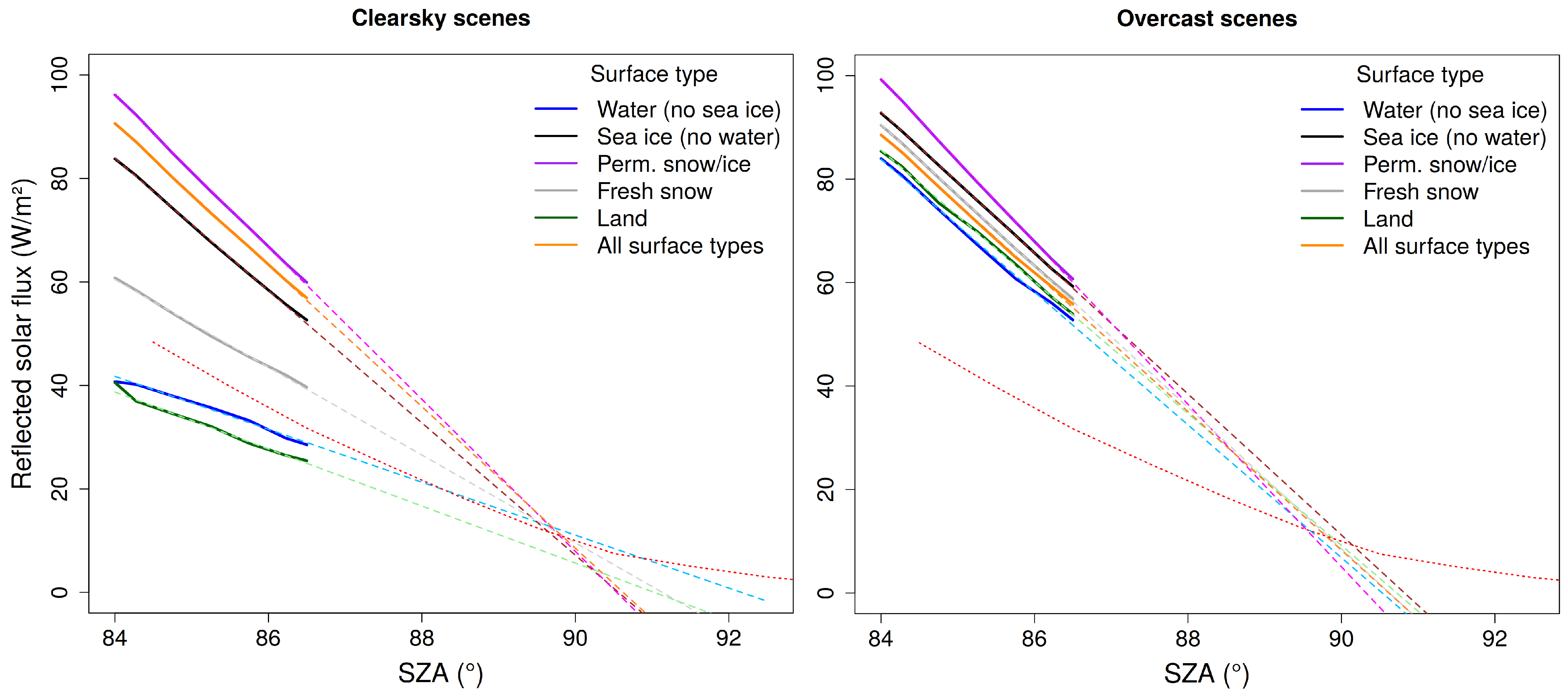
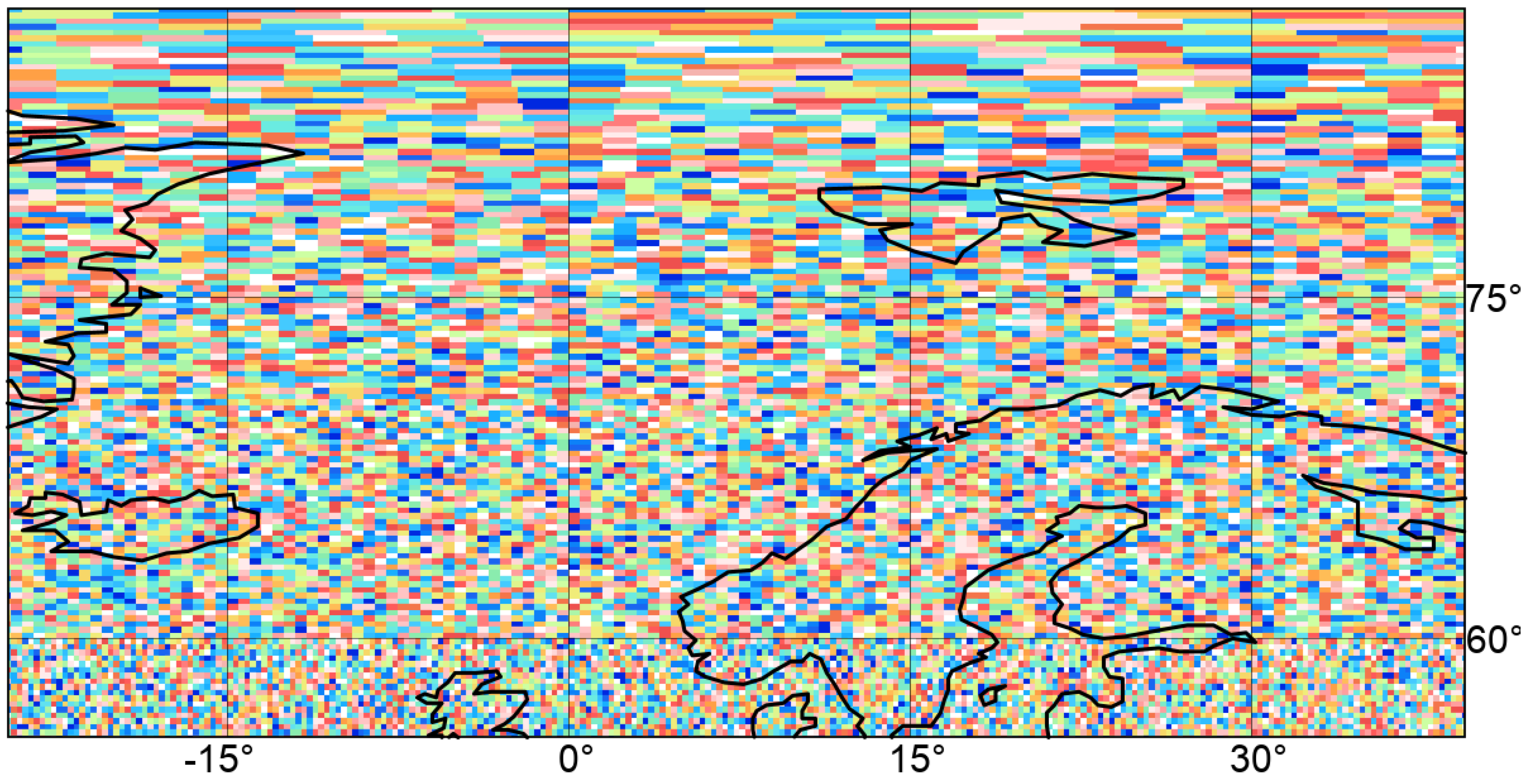
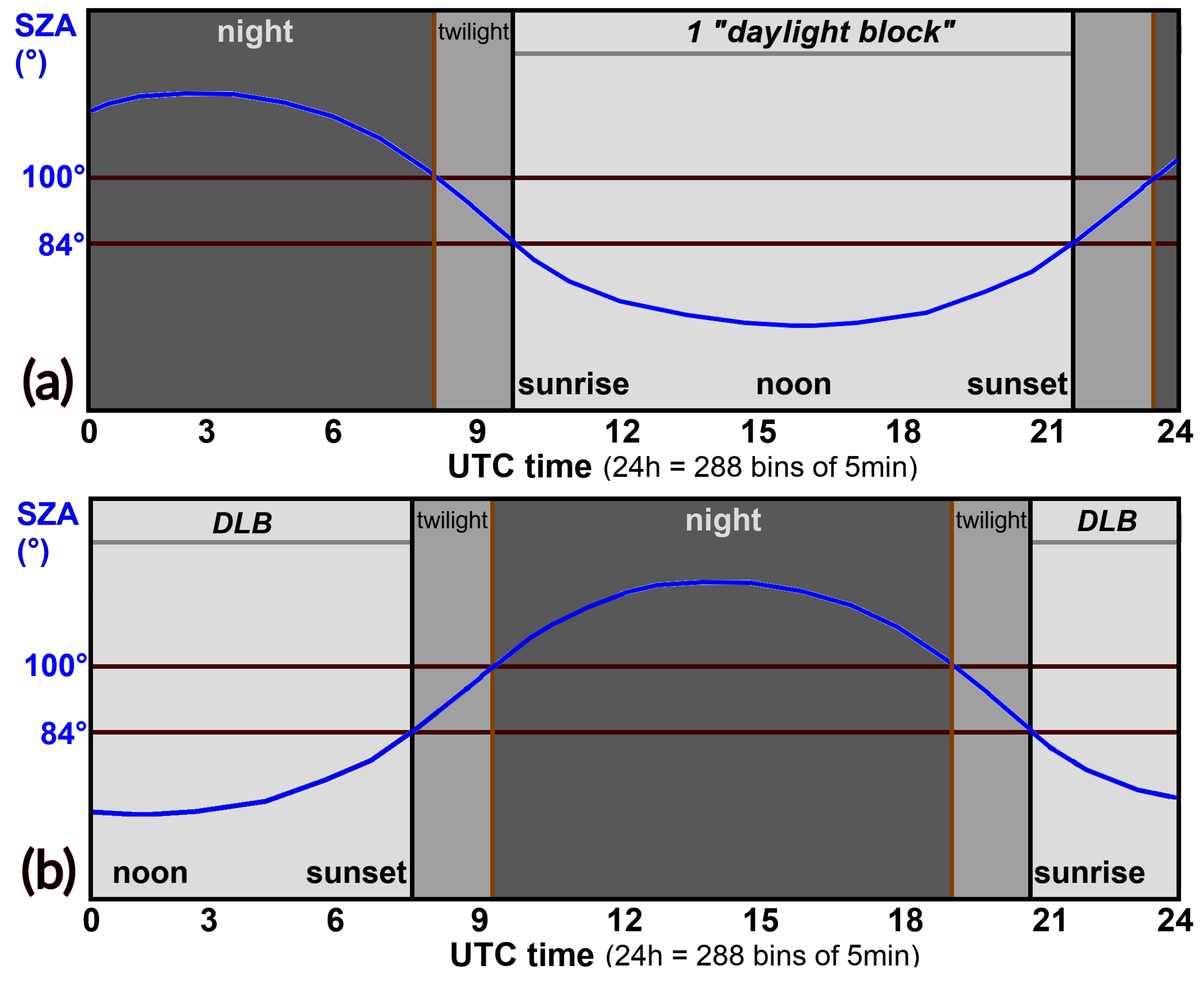
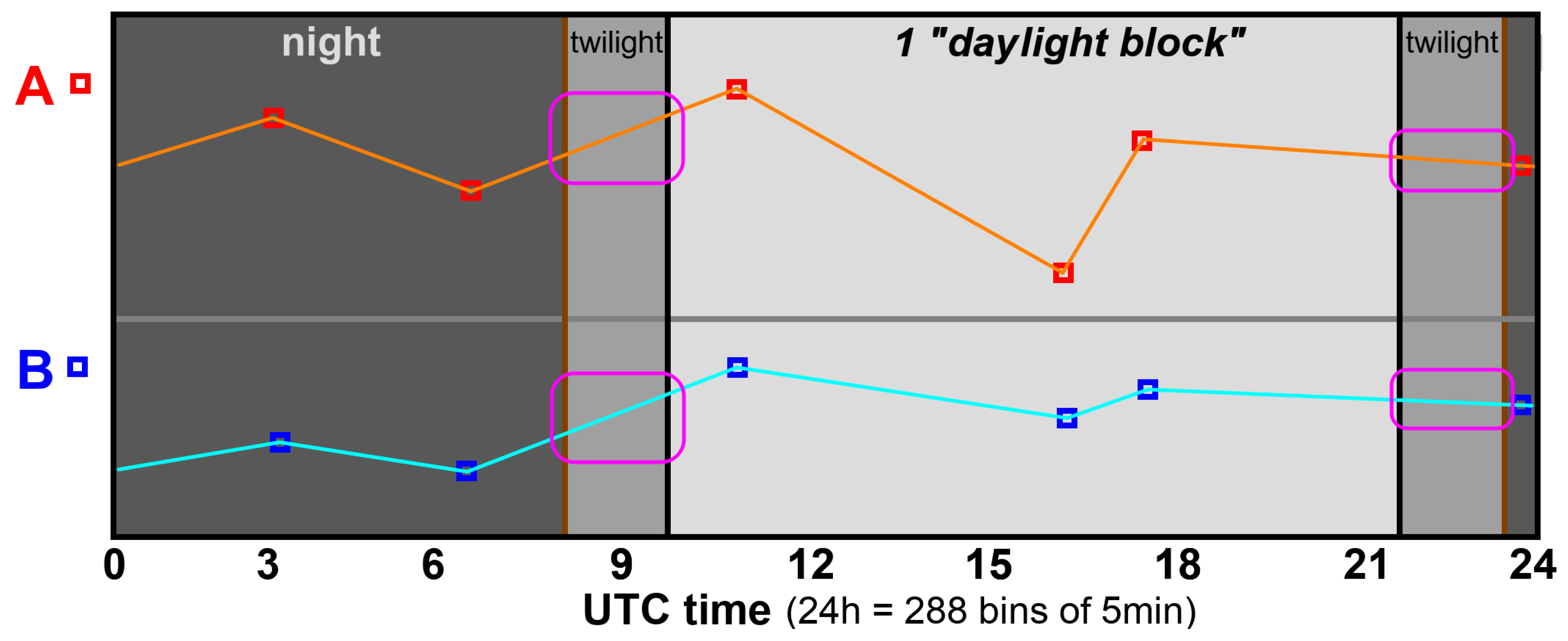
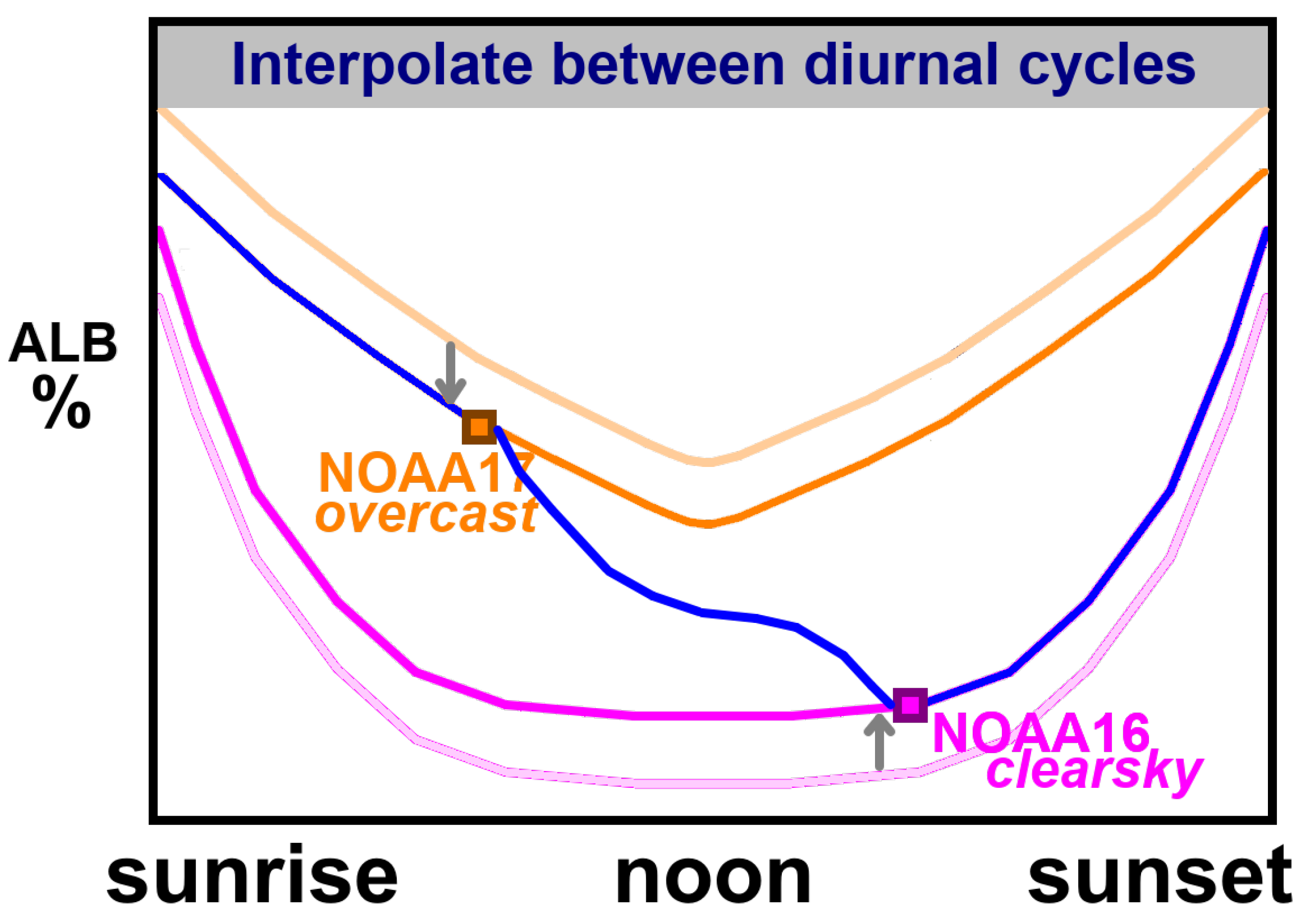
The third part of the TOA flux retrieval consisted of temporally integrating all available instantaneous observations for a given day, which makes it a multi-satellite product. Figure 2a shows the different orbits as a function of local solar time: typically there is at least one (mid-)morning and one afternoon observation, and depending on latitude this may be complemented by an early morning and/or late afternoon observation. This section describes how all these instantaneous albedo observations are fused together to construct a daily mean value.

For each nested 0.25${}^{\circ }$ grid box, the UTC day (24 h) was subdivided in 288 temporal bins of 5 min each (referred to as 5 min bins). For each of these temporal 5 min bins, the solar zenith angle was calculated based on the grid box’s location and time in the 5 min bin center. The day was subdivided into three types of 5 min bins (Figure 7a): (1) daylight bins, for which ${\theta }_0<{84}^{\circ }$, cf. Section 3.3.1, (2) twilight bins, for which 84${}^{\circ }\le {\theta }_0<{100}^{\circ }$, cf. Section 3.3.2, and (3) nighttime bins, for which ${\theta }_0\ge {100}^{\circ }$, cf. Section 3.3.3.

3.3.1. Daylight Conditions (${\theta }_0<{84}^{\circ }$): Modeling Albedo Diurnal Cycle

A consecutive time period of 5 min bins with daylight conditions (${\theta }_0<{84}^{\circ }$) is called a “daylight block (DLB)” (Figure 7a). Depending on the grid box’s location and season, a single UTC day may contain zero, one, or two DLBs. Each DLB was processed separately.

All the remapped Level-2b observations (output from Section 3.2) of previous, current, and next UTC day were collected, and only those were selected from which the observation’s time stamp falls within the temporal range of the daylight block. Each observation was assigned to the temporally nearest 5 min bin. In cases where more than one observation fell within the same 5 min bin, priority was given to the observation with the lowest temporal difference with the 5 min bin center.

The temporal interpolation method used here, called the “constant meteorology method”, has been documented extensively by Young et al. [42] and used subsequently in the CERES processing, where it is also called the “CERES-only (CO) method” [41]. An illustrative example for a hypothetical DLB is shown in Figure 8, showing a DLB with two observations, in this case from NOAA-17 and NOAA-16. Each observation has an associated scene type, that is, a combination of surface type and cloud properties (cover, phase, optical thickness).

An iteration was started over all observations in the DLB. The scene type of each observation was used to select its corresponding albedo model, which describes the variation of TOA albedo depending on solar zenith angle ${\theta }_0$ (Section 2.1). Each 5 min bin of the DLB has its own ${\theta }_0$ (Figure 7a), and hence can be assigned an albedo value based on the selected albedo model, resulting in a diurnal cycle. In Figure 8 this is shown for the first observation (NOAA-17; overcast) by the light orange curve.

The diurnal cycle’s albedo should not be too far off the observed albedo, but there will be a difference in most cases because the albedo model provides an average value and not an instantaneous observation. However, rather than the absolute magnitude, it is mostly the shape of this curve which is important. Therefore, the diurnal cycle curve (from the albedo model) was scaled to match the observation, as shown by the dark orange curve in Figure 8. This was done by calculating the ratio between observed and modeled albedo, and applying it to scale the entire diurnal cycle (Equation (4) in [42]).

Some situations require additional corrections. For instance when an observation around solar noon has a relatively high observed albedo but due to errors in the auxiliary input data, the diurnal cycle is much lower and more curved. The scaling could then lead to erroneous albedo values, exceeding 100% around sunrise and sunset. In these cases, iterative modifications were applied to the scene type, in steps of +25% cloud cover, and then, if needed, steps of +15 optical thickness, which ‘flatten’ the albedo model’s diurnal cycle and hence decrease the risk of excessive scaling (which would lift albedo’s over 100%). As soon as the (iteratively modified) diurnal cycle does not exceed 100%, it is accepted.

The iteration then proceeded to the next observation, in this example NOAA-16 with a clear-sky scene type. The same steps were applied to this observation, that is, determination of the albedo model’s diurnal cycle (light pink curve in Figure 8) and scaling of the albedo model’s diurnal cycle (dark magenta curve in Figure 8).

The final step consists of interpolating between the scaled diurnal cycles. This was done for each 5 min bin as a linear mean of the cycles corresponding to the closest preceding and closest following observation. This method assumes that the scene types (cloud properties) evolve linearly between the observations. From sunrise to the first observation, and after the last observation until sunset, there was no interpolation and a single scaled diurnal cycle was used. The final result was obtained by connecting the interpolated diurnal cycles, cfr the blue curve in Figure 8.

In the example of Figure 7a and Figure 8, the DLB was entirely situated within the 24 h temporal range of the UTC day, and hence, only a single DLB contributed to the daily mean calculation. However, for part of the globe (centered around the antimeridian) the UTC day contained two partial DLBs, typically with the first DLB containing 0 h UTC and the second DLB containing 24 h UTC (Figure 7b). In these cases, an additional last step was required (after the TOA albedo has been interpolated), that is, cutting off the redundant part(s) of the diurnal cycle that did not belong to the current UTC day.

Finally, for every 5 min bin in the DLB, the albedo (${\alpha }_{SW}$) was converted to daylight flux $F_{daylight}$ (Wm${}^{-2}$) as follows:

$$F_{daylight}=\left(\frac{{\alpha }_{SW}·TSI·cos\left({\theta }_0\right)}{d^2}\right)·{\left(\frac{r_e}{r_e+h_{20}}\right)}^2.$$

(6)

The first term contains the daily Total Solar Irradiance (TSI, Wm${}^{-2}$) supplied as input data cfr. Section 2.1. The Sun–Earth distance (d) was calculated using the Bretagnon method and coefficient look-up tables [43]. The second term in Equation (6) is a correction to scale the reference level of the flux to 20km, according to Loeb et al. [35] (Equation (18) in that reference), and equals 0.993751 ($r_e$ is the Earth’s equatorial radius).

If the DLB did not contain any observations, the entire daily mean was flagged as invalid. This may happen because the Level-2 input data is corrupted or invalid. Another, more frequent reason is that the duration of the DLB is very short, typically occurring in wintertime at high latitudes, which decreases the chance of having an observation falling within its temporal range. To avoid too many daily mean grid boxes being flagged as invalid, an exception was made for these situations: if the minimum solar zenith angle (${\theta }_0$) remained higher than 80${}^{\circ }$ over the entire DLB, all its 5 min bins would be re-categorized to “twilight” and processed as such (Section 3.3.2), meaning that the twilight model was exceptionally extended to the range of 80${}^{\circ }<{\theta }_0<{84}^{\circ }$. This exception is a trade-off between data coverage (avoiding too much missing grid boxes) and accuracy (not relying too much on modeling by setting requirements to the minimum contribution of observations).

In the example of Figure 8, there would be two shortwave instantaneous Level-2b observations used to create the albedo’s diurnal cycle (one from NOAA-17 and one from NOAA-16) from only one DLB. Note that in the case of multiple DLBs, these were added and the total number was higher. An example for the daily mean of 23 July 1983 is shown in Figure 2b. Latitudinal variation is seen in the winter hemisphere (here South) which is characterized by shorter daylight blocks, that is, by more observations falling outside the DLBs limits. In the northern hemisphere, the dominant feature is an increase towards the pole due to overlapping orbits. Furthermore, there is longitudinal variation due to: (1) number of DLBs per UTC day—because each DLB should have at least one observation, regions with two DLBs have at least two observations; and (2) sideways overlap of consecutive orbits, that is, where the swath edges of each orbit overlap with the edges of next orbit, resulting in a double temporal frequency compared to the center part of the swath. Similar to the latitudinal sampling variation due to overlapping orbits, this is considered an inherent feature of polar orbiting satellite processing, and the increased temporal sampling was fully used (i.e., there was no selection) since it increased the observational impact of the diurnal cycle compared to the modeling/interpolation impact.

3.3.2. Twilight Conditions (${84}^{\circ }\le {\theta }_0<{100}^{\circ }$)

The typical AVHRR/MetOp constellation does not have any orbits near the terminator, and consequently (sub-)tropical and midlatitude regions lack observations around sunrise and sunset (i.e. twilight). The discretized ${\theta }_0$-dependent albedo models that were used to interpolate the RSF diurnal cycle during daytime (Section 3.3.1) are not suitable for extrapolation beyond solar zenith angles of 84${}^{\circ }$. In (sub-)Polar regions, however, observations near the terminator are common, but the low illumination conditions make observation-based RSF retrievals difficult, for instance it complicatesthea proper scene type identification required for the narrowband-to-broadband conversion and for the ADM.

Hence, rather than relying on observations, RSF in twilight conditions needs to be simulated using a model. Such models can simulate the physical processes, for example, RTMs. However, their disadvantages, as mentioned in Section 1, are only aggravated in twilight conditions: first, the computational complexity increases (it becomes harder to achieve stable solution for the equations); furthermore, the illumination geometry becomes fully three-dimensional which requires a different kind of calculation and input data (e.g., cloud profiles); also, the nature of the required parameters changes, for example, surface parameters become less important at the cost of atmospherical parameters. Finally, radiative transfer simulations in twilight conditions should account for the Earth’s curvature and the Earth’s tangent radiation (radiation that goes through the atmosphere without touching the surface). These effects are not simulated in most of the (plane parallel) radiative transfer models.

The above mentioned obstacles were avoided by making use of a ${\theta }_0$-dependent empirical twilight model which needs very few input data (static surface map and easily retrievable binary cloud mask).

In contrast to the Level-2 albedo retrieval, the twilight coefficients A (intercept) and B (slope) (Table 2) were calculated for each observation, regardless of day- or nighttime. This was done based on its observed scene type, that is, the combination of TWL surface type (Table 4) and cloud cover. There was no cloud cover weighting, since the cloud mask is binary (either overcast or clear-sky). However, for surface type there is some need for weighting, more specifically for the sea ice: the TWL surface type “(1) sea ice, 100%” is for pure sea ice surfaces. Hence, a weighted average was made for sea ice and water depending on their relative areal share of sea ice in the pixel.

For each observation, the associated twilight coefficients were assigned to the temporally closest 5 min bin (Figure 9). Because the pixel’s scene type may vary between subsequent observations throughout the day (changing cloud cover, sea ice concentration), these scene type dependent coefficients were linearly interpolated (orange and cyan lines in Figure 9).

Finally, for each twilight 5 min bin (purple boxes in Figure 9), a flux was calculated ($F_{twilight}$; Wm${}^{-2}$) by combining the interpolated A and B coefficients with their corresponding bin-specific Solar Zenith Angle (${\theta }_0$, degrees) in Equation (1). When the result was lower than the all-sky twilight model by Kato and Loeb [37], cfr. the dotted lines in Figure 3, it was matched to the latter. This was done because the linear Flux-${\theta }_0$ relation is not valid anymore for very small fluxes (${\theta }_0>{90}^{\circ }$) where it is characterized by a smooth asymptotic transition to the nighttime zero flux.

3.3.3. Nighttime Conditions (${\theta }_0>{100}^{\circ }$)

For all the 5 min bins with nighttime conditions (${\theta }_0>{100}^{\circ }$) the flux was set to zero.

$$F_{night}=0.0{\mathrm{Wm}}^{-2}.$$

(7)

3.3.4. Daily Integral

The daily mean Reflected Solar Flux ($F_{daily}$; Equation (8)) was calculated by taking the average of all 5 min bins that had been processed either with conditions for daylight ($F_{daylight}$, Section 3.3.1), twilight ($F_{twilight}$, Section 3.3.2) or nighttime ($F_{night}$, Section 3.3.3), with the number of contributing 5 min bins for the three components being respectively I, J and K. As the UTC day has 288 temporal 5 min bins, it follows that $I+J+K=288$.

$$F_{daily}=\frac{1}{I+J+K}·\left(\sum _{i=1}^I{F}_{daylight,i}+\sum _{j=1}^J{F}_{twilight,j}+\sum _{k=1}^K{F}_{night,k}\right).$$

(8)

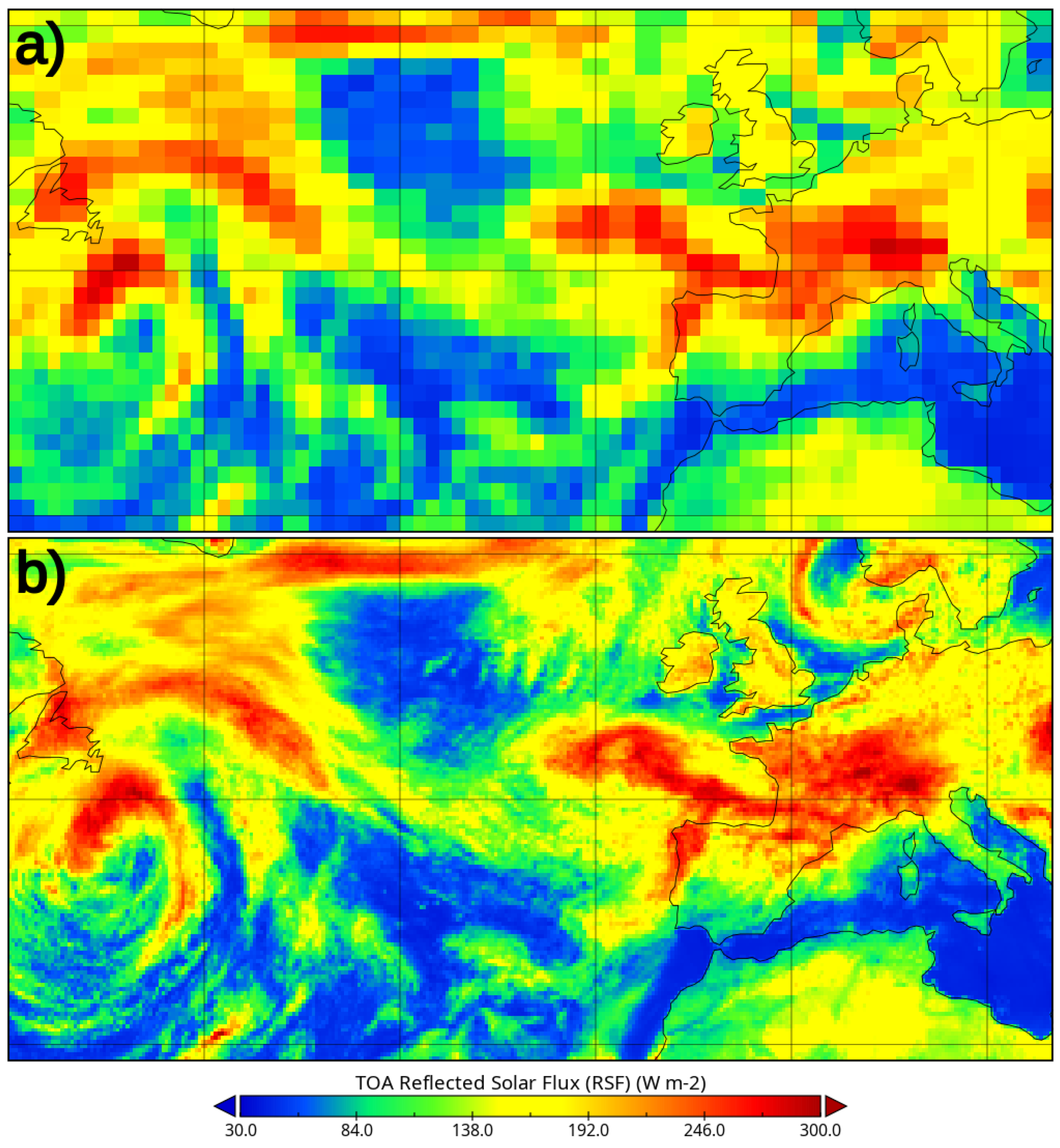
4. Results and Validation

Results and validation are shown here for the year 2008, for which all input data are made available in the preparatory test phase of the CLARA-A3 data record.

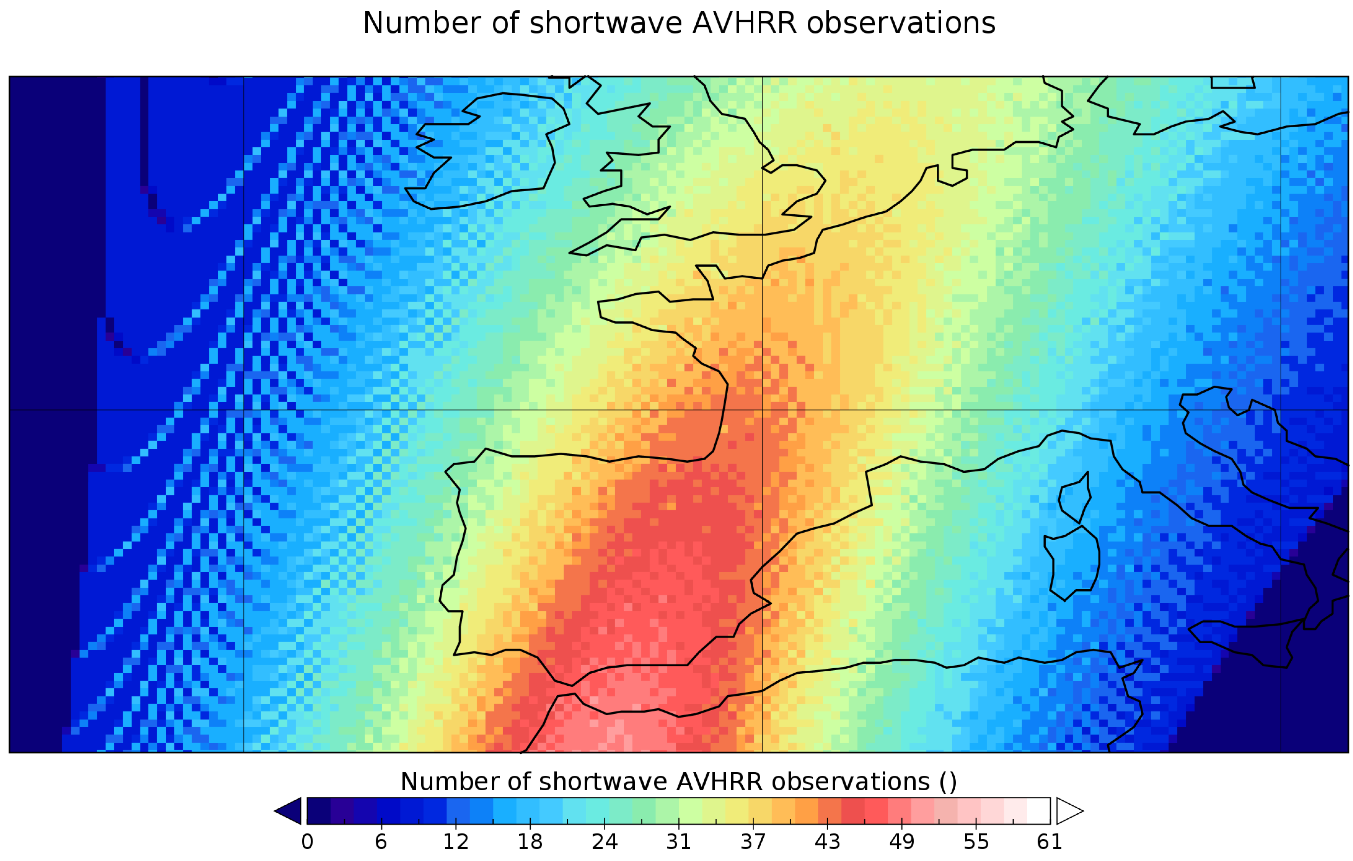
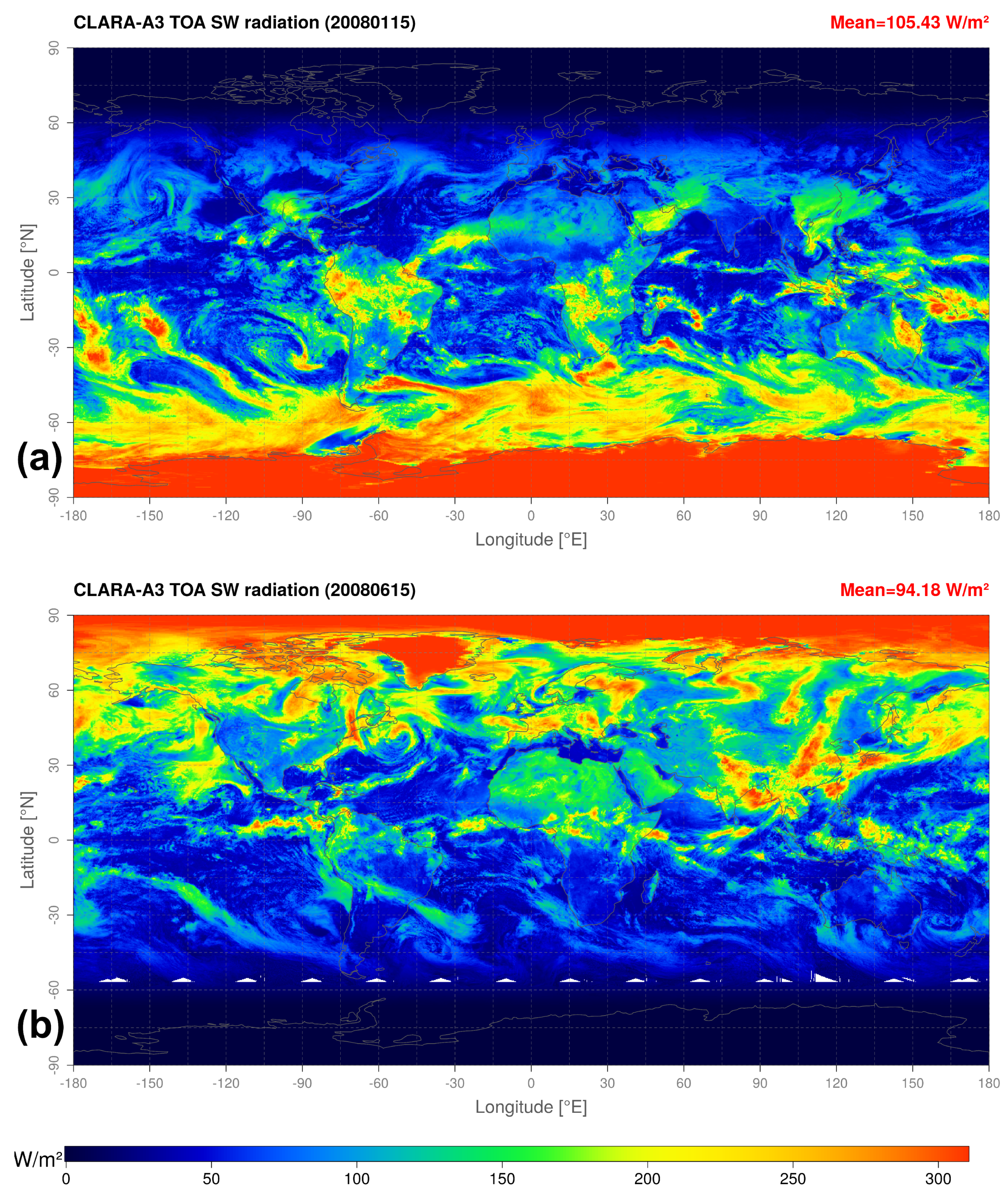
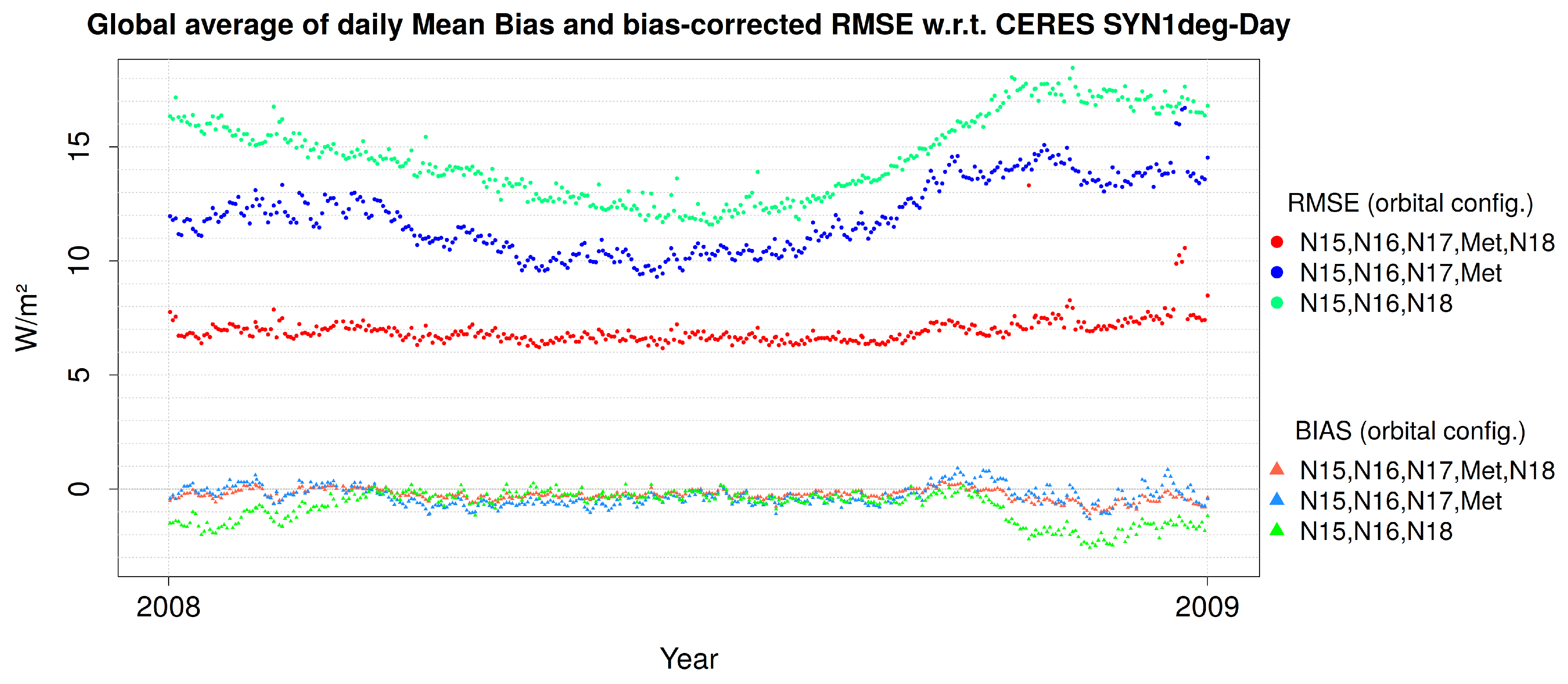
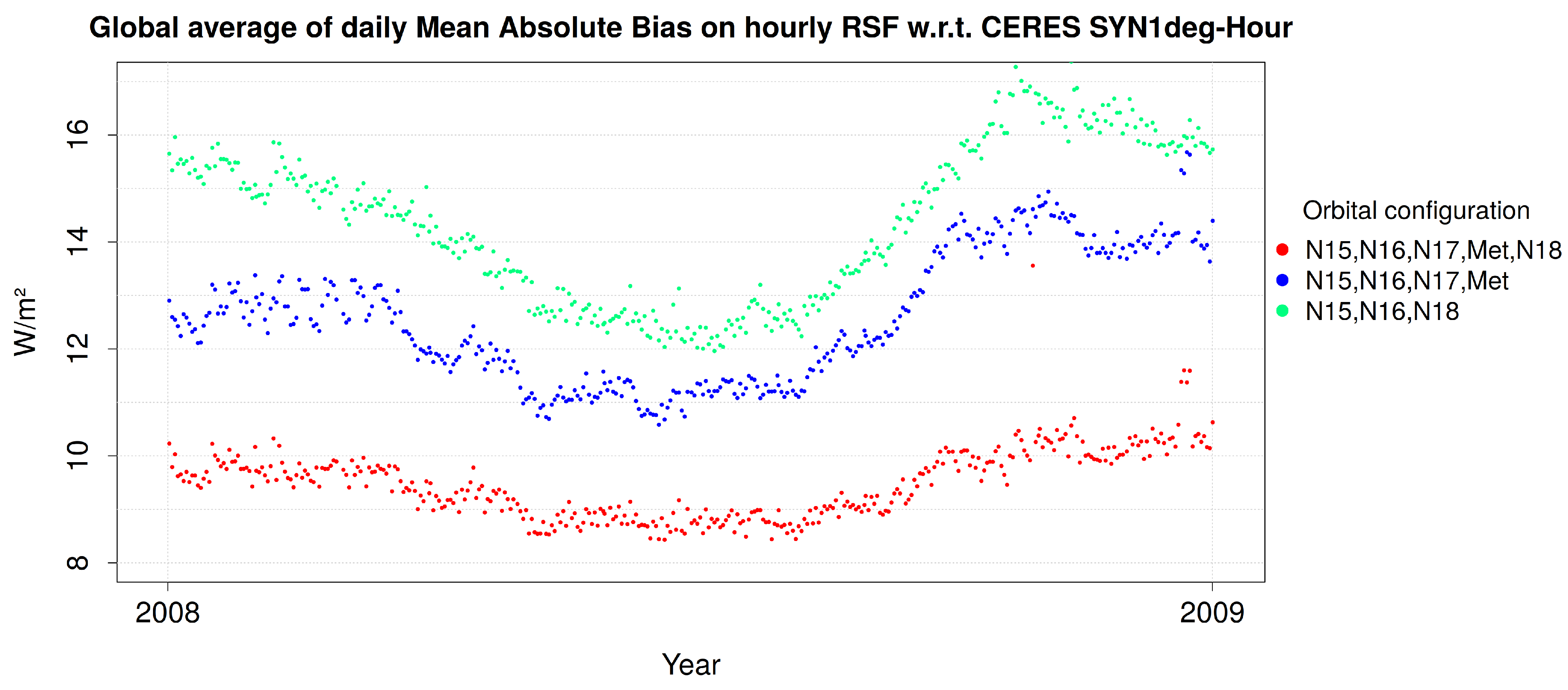
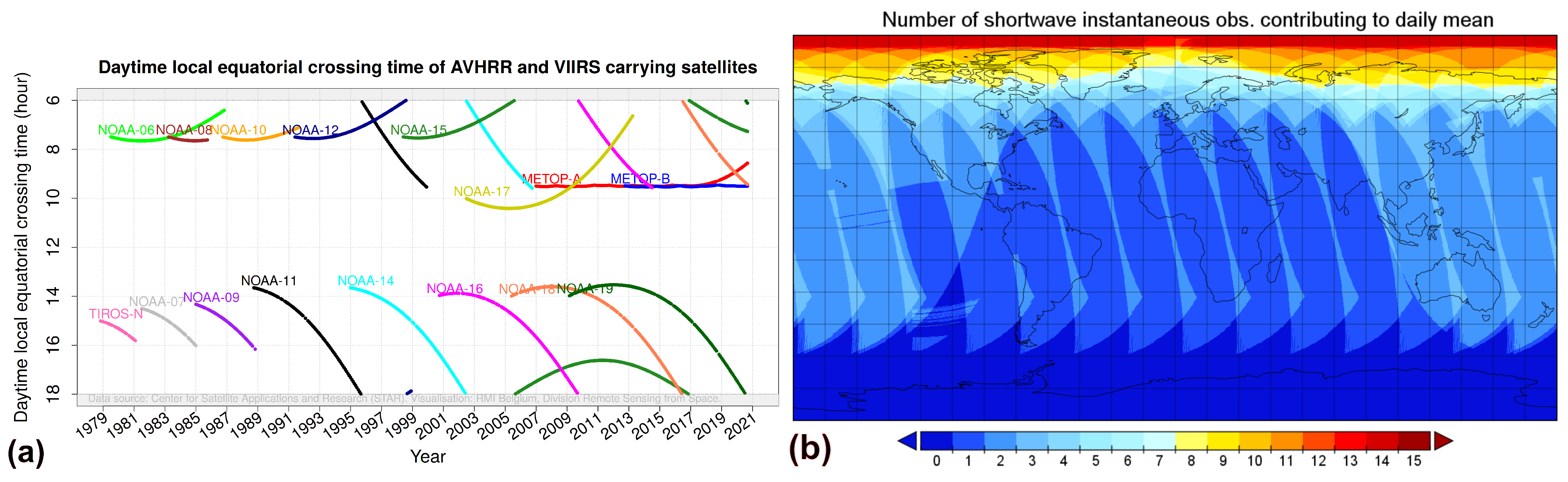
4.1. Orbital Configurations

The year 2008 is characterized by an AVHRR-carrying constellation of five satellites (Figure 2a), each with a specific semi-constant local equatorial crossing time: NOAA-15 (~5 h,~17 h), MetOp-A (~9 h30), NOAA-17 (~10 h), NOAA-18 (~13 h30), and NOAA-16 (~4 h30,~16 h30). Most important are the (mid-)morning (MetOp,NOAA-17) and early afternoon (NOAA-18) orbits, since these observations have superior illumination conditions and are generally better suited for temporally interpolating the diurnal cycle, compared to early morning or late afternoon observations. A big challenge of the Level-3 TOA flux retrieval is to capture the diurnal variability, which depends on the dominant regional climate features. Features that exhibit systematic asymmetry around solar noon especially require observations during both morning and afternoon (e.g., marine stratocumulus clouds that “burn off” during the afternoon).

On time scales longer than the particular year 2008, this orbital configuration is subject to orbital drift and eventually phasing out of some satellites, as well as their replacement with new satellites which keep the orbital configuration more or less similar until about 2016. However, during its drift towards an evening orbit from 2016 onwards (Figure 2a), the most recent early afternoon AVHRR instrument has not been replaced because it was the last produced piece of its series (NOAA-19); the Visible Infrared Imaging Radiometer Suite (VIIRS) instrument has been mounted on the new satellites instead. For data records exclusively relying on AVHRR observations, this has a considerable impact, which is estimated here by performing the validation for different orbital configurations. Besides the default configuration, using all available satellites, an alternative configuration was validated, which excludes the early afternoon satellite NOAA-18 and thus mimics the post-drift NOAA-19 situation.

Furthermore, the added value of mid-morning orbits can be estimated by excluding NOAA-17 and MetOp. The mid-morning orbits were considered together, as they are almost simultaneous in local equatorial crossing time and hence do not provide a lot of added value with respect to each other. Their removal anticipates the future situation when the MetOp satellites will be decommissioned.

Finally, five additional configurations consist of each satellite separately, to estimate their relative importance. Early morning or late evening satellites do not provide global coverage, as the day length determines whether these observations can be used that early (or late) on a given UTC day, which in turn depends on the latitude and season. An overview of all the tested orbital configurations is given in Table 5.

Two daily means from 15th January and 15th June, retrieved using all available satellites, are shown in Figure 10 to illustrate the level of detail and realism of the obtained TOA flux.

4.2. Validation Approach and Performance Indicators

The retrieved daily mean CLARA-A3 RSF ($F_{CLARA}$) was validated against the daily mean TOA Shortwave Flux from the CERES synoptic gridded product SYN1deg [44] edition 4.1, denoted by $F_{CERES}$. Note that CERES’ Energy Balanced and Filled (EBAF) product [32] was not used since it is a monthly product optimized regarding absolute accuracy (calibration), stability, and long term (decadal) trend detection, whereas this validation was done on daily and sub-daily scale.

The bias of daily mean RSF for every grid box with indices $(i,j)$ was calculated as $F_{CLARA,i,j}-F_{CERES,i,j}$. Prior to the validation, the spatial resolution of $F_{CLARA}$ was first downgraded to match the nested grid of CERES. Maps of this bias were created (daily “bias maps”), from which the global Mean Bias ($MB$) and corresponding bias-corrected RMS of the bias ($RMSB$) were calculated over all grid boxes’ biases, as follows:

$$MB=\frac{1}{m·n}·\sum _{i=1}^m\sum _{j=1}^n(F_{CLARA,i,j}-F_{CERES,i,j})$$

(9)

$$RMSB=\sqrt{\frac{1}{m·n}·{\sum }_{i=1}^m{\sum }_{j=1}^n{(F_{CLARA,i,j}-F_{CERES,i,j}-MB)}^2},$$

(10)

where m and n are the number of grid boxes in longitude (360) and latitude (180) dimension, respectively. The $RMSB$ is a commonly used measure of spatial validation between data records, or with respect to a reference record (considered truth), also called regional uncertainty (precision). The $MB$ is a measure for the absolute calibration of the data record with respect to the reference data (accuracy). Note that these global statistics were calculated using a latitudinal area weighting to prevent an over-representation of the polar areas, which is not shown in the simplified equations to preserve readability.

Besides the $MB$ and $RMSB$, the absolute bias of daily mean RSF for every grid box $(i,j)$ was calculated as $\left|F_{CLARA,i,j}-F_{CERES,i,j}\right|$. Similar to the mean bias (Equation (9)), the Mean Absolute Bias ($MAB$) was then calculated as the global spatial mean over all grid boxes, as shown in Equation (11). The daily $MAB$ is another measure for regional uncertainty.

$$MAB=\frac{1}{m·n}·\sum _{i=1}^m\sum _{j=1}^n\left|F_{CLARA,i,j}-F_{CERES,i,j}\right|.$$

(11)

The above mentioned performance indicators ($MB$, $RMSB$ and $MAB$) are based on biases between daily mean quantities (daily mean RSF from CLARA-A3 and daily mean RSF from CERES-SYN1deg). Therefore, these indicators may be hiding (temporal) intra-day compensating errors, for instance an overestimation in the morning followed by an underestimation in the afternoon which cancel each other, resulting in an apparently low bias for a given grid box. This was investigated by calculating the $MAB$ on hourly time scale ($MABH$) between the retrieved dataset (CLARA-A3) and the reference dataset (CERES SYN1deg-Hour Ed.4.1). The daily absolute bias on an hourly time scale for a single grid box $(i,j)$ was thus calculated from 24 h, denoted h, and hence 24 biases (Equation (12)). From this, the spatial global mean was calculated to obtain the $MABH$:

$$MABH=\frac{1}{m·n}·\sum _{i=1}^m\sum _{j=1}^n\left[\frac{1}{24}·\sum _{h=1}^{24}\left|F_{CLARA,i,j,h}-F_{CERES,i,j,h}\right|\right].$$

(12)

All the mentioned performance indicators are so-called “indicators of dispersion (Class A)” in the terminology of Gueymard [45]. The use of more sophisticated indicators is beyond the scope of this article, in which the validation primarily serves as a first confirmation of the retrieval algorithm’s capabilities following the preparatory test phase of CLARA-A3 (with only one year of data). However, once the full data record is generated and released, a more extensive in-depth validation will be performed.

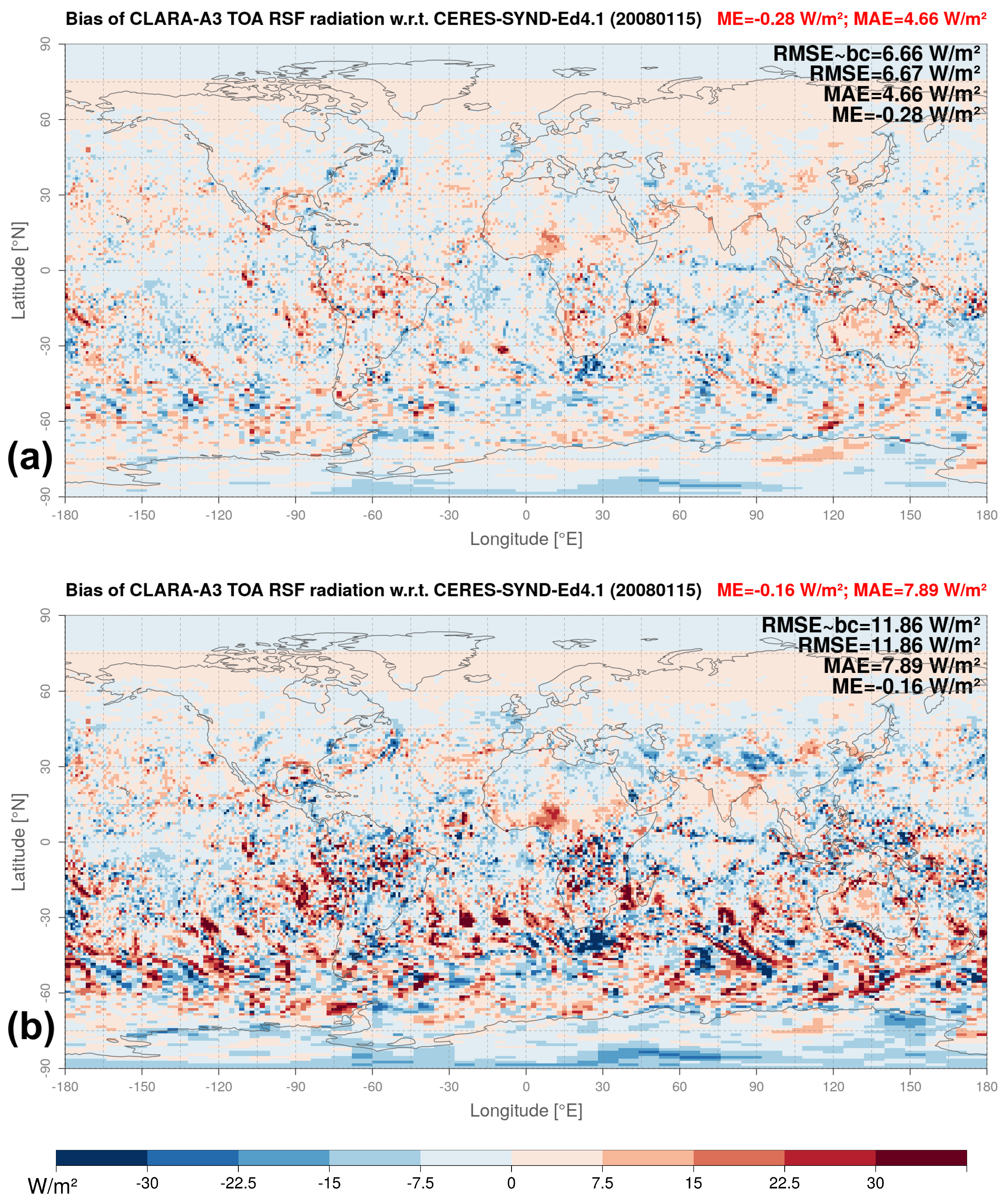
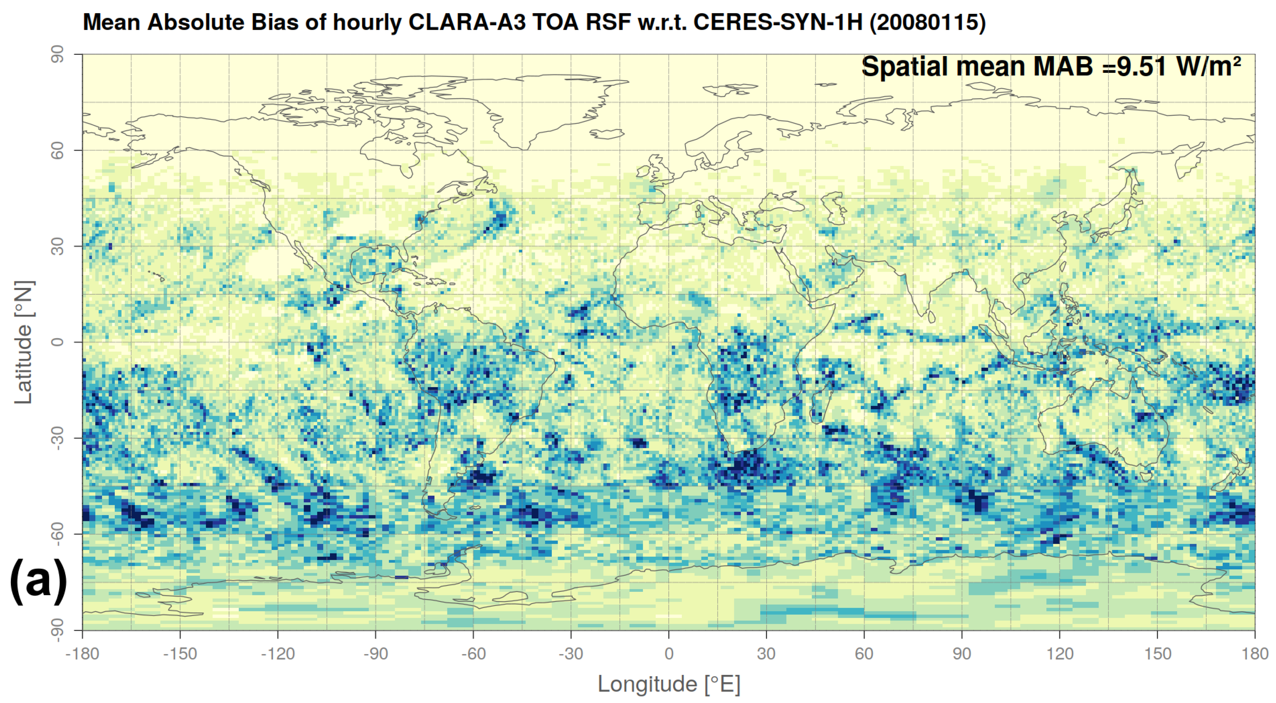
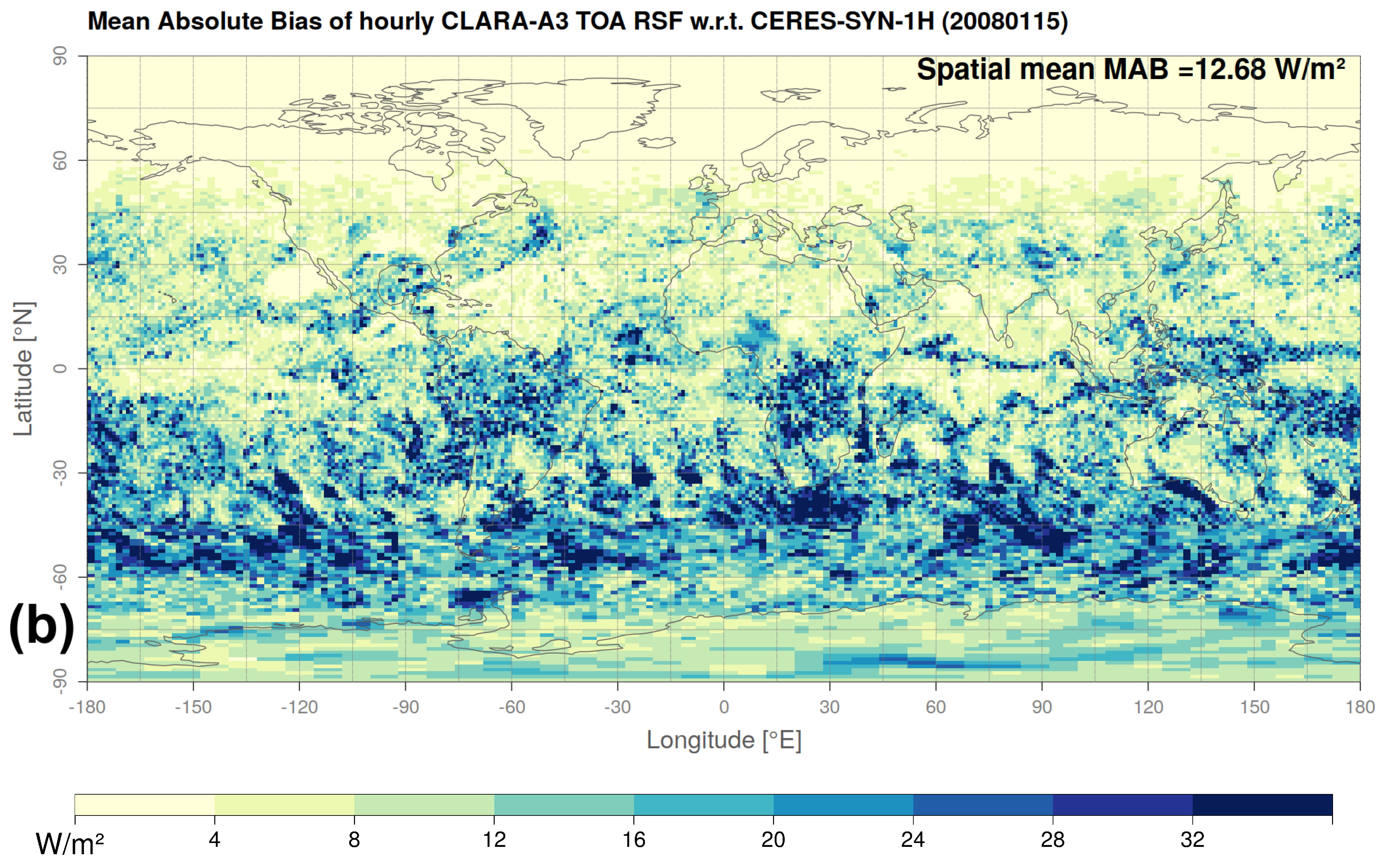
4.3. Validation on Daily Time Scale

An example of the calculated daily “bias maps” is shown in Figure 11a, whose date corresponds to Figure 10a (15 January 2008). With the default orbital configuration, most regions are characterized by a daily mean bias within +/−7.5 Wm${}^{-2}$ (Figure 11a). As expected, the largest biases can be found in regions with highly dynamic weather systems (requiring frequent temporal sampling), and are in general also related to RSF’s absolute magnitude (driven by insolation and reflectance). The configuration without early afternoon orbit (Figure 11b) has several regions with pronounced biases (+/−30 Wm${}^{-2}$), often consisting of swirls with positive alongside negative bias.

The configuration using all satellites is characterized by a stable mean bias ($MB$) around 0 Wm${}^{-2}$ (red triangles in Figure 12). The bias corrected RMSB also shows a relatively stable performance of about 7 Wm${}^{-2}$ (red dots in Figure 12). The annual average of these statistics is shown in Table 5, where the colors refer to the same configurations used in Figure 12.

The configuration excluding NOAA-18, that is, without early afternoon orbit (blue in Figure 12), has a significantly degraded performance, with a bias corrected RMSB ranging seasonally between 10 and 14 Wm${}^{-2}$, which is about 12 Wm${}^{-2}$ annually (Table 5). Excluding the mid-morning orbits (NOAA-17 and MetOp-A) causes the RMSB to increase even more, to 12–18 Wm${}^{-2}$ (green in Figure 12), with an annual average of 14.6 Wm${}^{-2}$ (Table 5). The mean bias is less stable, with seasonal deviations up to −2 Wm${}^{-2}$ (light green triangles in Figure 12).

Table 5. Average annual validation statistics for different orbital configurations, during year 2008. The colored configurations refer to the ones in Figure 12.

Orbital Configurations					Annual Average of Daily Statistics (Wm${}^{-2}$)
Early/Late		Midmorning		Aftern.	$\mathit{MB}$	$\mathit{RMSB}$	$\mathit{MAB}\left(\mathit{H}\right)$
N15	N16	Met	N17	N18	***	***	Daily **	Hourly **
x	x	x	x	x	−0.27	6.93	4.83	9.47
		x	x	x	−0.14	7.20	4.91	9.24
x	x	x		x	−0.15	7.59	5.24	9.97
x	x		x	x	−0.31	7.18	5.01	9.76
x	x	x	x		−0.31	11.92	8.05	12.56
x	x			x	−0.76	14.63	9.62	14.42
				x	−0.33	15.56	10.01	14.40
			x		0.28	17.32	11.14	15.41
		x			0.65	18.50	11.87	16.11
	x *				−2.45	28.86	19.28	24.13
x *					0.39	30.40	20.02	25.07

* these orbits do not provide complete global coverage; to be interpreted with care. ** Mean Absolute Bias (MAB) is calculated on both daily and hourly time scale. *** Mean Bias (and hence RMSB) are identical on daily and hourly timescale.

Table 5. Average annual validation statistics for different orbital configurations, during year 2008. The colored configurations refer to the ones in Figure 12.

Orbital Configurations					Annual Average of Daily Statistics (Wm${}^{-2}$)
Early/Late		Midmorning		Aftern.	$\mathit{MB}$	$\mathit{RMSB}$	$\mathit{MAB}\left(\mathit{H}\right)$
N15	N16	Met	N17	N18	***	***	Daily **	Hourly **
x	x	x	x	x	−0.27	6.93	4.83	9.47
		x	x	x	−0.14	7.20	4.91	9.24
x	x	x		x	−0.15	7.59	5.24	9.97
x	x		x	x	−0.31	7.18	5.01	9.76
x	x	x	x		−0.31	11.92	8.05	12.56
x	x			x	−0.76	14.63	9.62	14.42
				x	−0.33	15.56	10.01	14.40
			x		0.28	17.32	11.14	15.41
		x			0.65	18.50	11.87	16.11
	x *				−2.45	28.86	19.28	24.13
x *					0.39	30.40	20.02	25.07

* these orbits do not provide complete global coverage; to be interpreted with care. ** Mean Absolute Bias (MAB) is calculated on both daily and hourly time scale. *** Mean Bias (and hence RMSB) are identical on daily and hourly timescale.

Some additional orbital configurations were validated to test the performance sensitivity to individual satellites. First, the very early and very late orbits (NOAA-15 and NOAA-16) were excluded, resulting in only a small performance degradation (second row in Table 5). Furthermore, the mid-morning orbits were tested individually, by excluding each of them separately (third and fourth row in Table 5). The resulting performance was only slightly affected. Finally, the single-satellite configurations (last five rows in Table 5) were not able to achieve the performance obtained by any of the combination configurations. However, there are significant differences, with the best performance by the afternoon satellite ($RMSB$ of 15.5 Wm${}^{-2}$), followed by each of the mid-morning satellites (around 18 Wm${}^{-2}$), and at a large distance the early and late satellites (28–30 Wm${}^{-2}$).

The daily $MAB$ is another measure for regional uncertainty, and its annual average statistics (Table 5, third column) confirm the orbital-specific performance assessment obtained by $RMSB$ (second column).

4.4. Validation on Hourly Time Scale

Daily maps with mean absolute bias calculated on an hourly time scale ($MABH$) are shown in Figure 13. The maps are similar to the daily mean bias maps (Figure 11), also showing the bias patterns associated with dynamic weather systems, which significantly increase by excluding the early afternoon observation, with the absolute bias regionally exceeding 32 Wm${}^{-2}$ (Figure 13b).

The $MABH$ of each day is plotted in Figure 14 and its annual average is listed in Table 5 (fourth column). The resulting statistics exhibit orbital-dependent performance differences similar to those seen for the $RMSB$ and $MAB$ on a daily time scale: the default configuration, using all satellites, is characterized by a relatively stable performance with $MABH$ between 9–10 Wm${}^{-2}$. However, excluding the early afternoon orbit (NOAA-18) results in a year-round performance degradation, with $MABH$ ranging seasonally between 11–14 Wm${}^{-2}$. Exclusion of mid-morning orbits (NOAA-17 and MetOp-A) has an even worse impact, with $MABH$ ranging between 12–16 Wm${}^{-2}$. For the additional orbital configurations listed in Table 5, the configuration-specific performance differences echo those obtained with $RMSB$ and $MAB$ on a daily time scale.

5. Discussion

The retrieval of daily mean RSF performs well when all orbits are used, demonstrated by a global RMSB below 7 Wm${}^{-2}$ and a stable bias around 0 Wm${}^{-2}$.

The configuration without NOAA-18 results in several regions with pronounced biases (+/−30 Wm${}^{-2}$), often consisting of swirls with positive alongside negative bias, caused by the extrapolation of the mid-morning observation to the afternoon: this is problematic for fast moving small-scale or heterogeneous weather systems (e.g., fronts) or for large-scale weather phenomena with asymmetrical diurnal cycle (e.g., afternoon marine stratocumulus burn-off). The significantly degraded performance (RMSB of 12 Wm${}^{-2}$) stresses the important role of the early afternoon satellite in constructing the RSF diurnal cycle. A similar performance degradation is expected due to the orbital drift of NOAA-19 towards an evening orbit during 2016–2020. Even more important are the mid-morning orbits (NOAA-17 and MetOp-A), demonstrated by the even larger performance degradation when they are excluded (RMSB of 14.6 Wm${}^{-2}$). Loss of mid-morning AVHRR orbits is not expected in the near future, but should at some point occur after MetOp-C is decommissioned. Combined, these results demonstrate and quantify the added value of both early afternoon and mid-morning observations, proving them essential for capturing the diurnal variability and obtaining accurate daily mean RSF.

The fact that performance is only slightly affected by excluding only one of the two mid-morning orbits demonstrates that the added value of individual orbits is related to their temporal spread throughout the day. In other words, both orbits are “interchangeable” concerning the performance of the daily mean RSF. The negligible performance degradation following the exclusion of NOAA-15 or NOAA-16 shows that these very early and very late orbits provide little added value to the reconstruction of the diurnal cycle, which may be partly caused by their small impact on the diurnal cycle interpolation.

The difference between Mean Absolute Bias calculated on a daily time scale and an hourly time scale is indicative of the intra-day compensating error. It is limited and systematic (about 4.5 Wm${}^{-2}$), meaning that it does not cause or influence the orbital-specific performance assessment on a daily time scale from which the results and conclusions remain valid.

After the release of the full CLARA-A3 data record, the 42-year data record of TOA RSF will allow more in-depth analyses, including an assessment on the long term data series’ stability and radiometric calibration, for example, by cross-comparison of monthly mean RSF from all existing reference data records.

6. Conclusions

A methodology to obtain daily mean top-of-atmosphere RSF (Wm${}^{-2}$) from AVHRR is presented. The different steps consist of: (1) a narrowband-to-broadband conversion of the AVHRR reflectances using empirical regressions with CERES observations; (2) an anisotropy correction using ADMs resulting in hemispherical albedo; and (3) a temporal interpolation between the available instantaneous albedos using a flexible diurnal cycle model.

This methodology is subsequently demonstrated by validating a full year (2008) of RSF daily means with the CERES SYN1deg data record, both on daily and subdaily scales. Several orbital configurations are tested, each excluding particular satellites from the constellation. Early afternoon and mid-morning orbits are proven essential for the daily mean RSF retrieval.

References

1. GCOS. Systematic Observation Requirements for Satellite-Based Products for Climate (2011 Update): Supplemental Details to the Satellite-Based Component of the “Implementation Plan for the Global Observing System for Climate in Support of the UNFCCC”. Reference Document GCOS-154. WMO. 2011. Available online: www.wmo.int (accessed on 1 August 2021).
2. Dewitte, S.; Clerbaux, N. Measurement of the earth radiation budget at the top of the atmosphere—A review. Remote Sens. 2017, 9, 1143. [Google Scholar] [CrossRef] [Green Version]
3. Barkstrom, B.R. The earth radiation budget experiment (ERBE). Bull. Am. Meteorol. Soc. 1984, 65, 1170–1185. [Google Scholar] [CrossRef]
4. Wielicki, B.A.; Barkstrom, B.R.; Harrison, E.F.; Lee, R.B., III; Smith, G.L.; Cooper, J.E. Clouds and the Earth’s Radiant Energy System (CERES): An earth observing system experiment. Bull. Am. Meteorol. Soc. 1996, 77, 853–868. [Google Scholar] [CrossRef] [Green Version]
5. Harries, J.E.; Russell, J.; Hanafin, J.; Brindley, H.; Futyan, J.; Rufus, J.; Kellock, S.; Matthews, G.; Wrigley, R.; Last, A.; et al. The geostationary earth radiation budget project. Bull. Am. Meteorol. Soc. 2005, 86, 945–960. [Google Scholar] [CrossRef] [Green Version]
6. Kandel, R.; Viollier, M.; Raberanto, P.; Duvel, J.P.; Pakhomov, L.; Golovko, V.; Trishchenko, A.; Mueller, J.; Raschke, E.; Stuhlmann, R.; et al. The ScaRaB earth radiation budget dataset. Bull. Am. Meteorol. Soc. 1998, 79, 765–784. [Google Scholar] [CrossRef] [Green Version]
7. Hersbach, H.; Bell, B.; Berrisford, P.; Hirahara, S.; Horányi, A.; Muñoz-Sabater, J.; Nicolas, J.; Peubey, C.; Radu, R.; Schepers, D.; et al. The ERA5 global reanalysis. Q. J. R. Meteorol. Soc. 2020, 146, 1999–2049. [Google Scholar] [CrossRef]
8. Hogan, R.J.; Bozzo, A. A flexible and efficient radiation scheme for the ECMWF model. J. Adv. Model. Earth Syst. 2018, 10, 1990–2008. [Google Scholar] [CrossRef] [Green Version]
9. Young, A.H.; Knapp, K.R.; Inamdar, A.; Hankins, W.; Rossow, W.B. The international satellite cloud climatology project H-Series climate data record product. Earth Syst. Sci. Data 2018, 10, 583–593. [Google Scholar] [CrossRef] [Green Version]
10. Stengel, M.; Stapelberg, S.; Sus, O.; Finkensieper, S.; Würzler, B.; Philipp, D.; Hollmann, R.; Poulsen, C.; Christensen, M.; McGarragh, G. Cloud_cci Advanced Very High Resolution Radiometer post meridiem (AVHRR-PM) dataset version 3: 35-year climatology of global cloud and radiation properties. Earth Syst. Sci. Data 2020, 12, 41–60. [Google Scholar] [CrossRef] [Green Version]
11. Poulsen, C.A.; McGarragh, G.R.; Thomas, G.E.; Stengel, M.; Christensen, M.W.; Povey, A.C.; Proud, S.R.; Carboni, E.; Hollmann, R.; Grainger, R.G. Cloud_cci ATSR-2 and AATSR data set version 3: A 17-year climatology of global cloud and radiation properties. Earth Syst. Sci. Data 2020, 12, 2121–2135. [Google Scholar] [CrossRef]
12. Lee, H.T.; Gruber, A.; Ellingson, R.G.; Laszlo, I. Development of the HIRS outgoing longwave radiation climate dataset. J. Atmos. Ocean. Technol. 2007, 24, 2029–2047. [Google Scholar] [CrossRef] [Green Version]
13. Urbain, M.; Clerbaux, N.; Ipe, A.; Tornow, F.; Hollmann, R.; Baudrez, E.; Velazquez Blazquez, A.; Moreels, J. The CM SAF TOA radiation data record using MVIRI and SEVIRI. Remote Sens. 2017, 9, 466. [Google Scholar] [CrossRef] [Green Version]
14. Heidinger, A.K.; Straka III, W.C.; Molling, C.C.; Sullivan, J.T.; Wu, X. Deriving an inter-sensor consistent calibration for the AVHRR solar reflectance data record. Int. J. Remote Sens. 2010, 31, 6493–6517. [Google Scholar] [CrossRef]
15. Hollman, R.; Schlundt, C.; Finkensieper, S.; Raspaud, M.; Karlsson, K.G.; Stengel, M. Technical Report on AVHRR GAC FCDR Generation. Technical Report Issue 1, Revision 0, ESA Cloud cci. 2017. Available online: http://www.esa-cloud-cci.org/sites/default/files/upload/Cloud_cci_RAFCDR_v1.0.pdf (accessed on 1 August 2021).
16. Abel, P.; Gruber, A. An Improved Model for the Calculation of Longwave Flux at 11 um. NOAA Technical Memorandum NESS 106. 1979. Available online: https://repository.library.noaa.gov/view/noaa/18548 (accessed on 1 August 2021).
17. Akkermans, T.; Clerbaux, N. Narrowband-to-broadband conversions for top-of-atmosphere reflectance from the Advanced Very High Resolution Radiometer (AVHRR). Remote Sens. 2020, 12, 305. [Google Scholar] [CrossRef] [Green Version]
18. Karlsson, K.G.; Riihelä, A.; Müller, R.; Meirink, J.; Sedlar, J.; Stengel, M.; Lockhoff, M.; Trentmann, J.; Kaspar, F.; Hollmann, R.; et al. CLARA-A1: A cloud, albedo, and radiation dataset from 28 yr of global AVHRR data. Atmos. Chem. Phys. 2013, 13, 5351–5367. [Google Scholar] [CrossRef] [Green Version]
19. Karlsson, K.G.; Anttila, K.; Trentmann, J.; Stengel, M.; Fokke Meirink, J.; Devasthale, A.; Hanschmann, T.; Kothe, S.; Jääskeläinen, E.; Sedlar, J.; et al. CLARA-A2: The second edition of the CM SAF cloud and radiation data record from 34 years of global AVHRR data. Atmos. Chem. Phys. 2017, 17, 5809–5828. [Google Scholar] [CrossRef] [Green Version]
20. Clerbaux, N.; Akkermans, T.; Baudrez, E.; Velazquez Blazquez, A.; Moutier, W.; Moreels, J.; Aebi, C. The Climate Monitoring SAF Outgoing Longwave Radiation from AVHRR. Remote Sens. 2020, 12, 929. [Google Scholar] [CrossRef] [Green Version]
21. Akkermans, T.; Clerbaux, N.; Karlsson, K.G.; Hollman, R. CM SAF Algorithm Theoretical Basis Document for Top-of-Atmosphere Products from the CMSAF Cloud, Albedo, Radiation Data Record, AVHRR-Based, Edition 3 (CLARA-A3). SAF/CM/RMIB/ATBD/GAC/TOA, Issue 1, Rev 0. 27 April 2021. EUMETSAT Satellite Application Facility on Climate Monitoring (CM SAF); Prepared by Royal Meteorological Institute Belgium (RMIB). 2021. Available online: www.cmsaf.eu; ftp://gerb.oma.be/tomakker/ATBD-TOA.pdf (accessed on 1 August 2021).
22. Devasthale, A.; Raspaud, M.; Schlundt, C.; Hanschmann, T.; Finkensieper, S.; Dybbroe, A.; Hörnquist, S.; Håkansson, N.; Stengel, M.; Karlsson, K. PyGAC: An open-source, community-driven Python interface to preprocess more than 30-year AVHRR Global Area Coverage (GAC) data. GSICS Quartherly Newsl. 2018, 11, 3–5. [Google Scholar]
23. Dybbroe, A.; Karlsson, K.G.; Thoss, A. NWCSAF AVHRR cloud detection and analysis using dynamic thresholds and radiative transfer modeling. Part I: Algorithm description. J. Appl. Meteorol. 2005, 44, 39–54. [Google Scholar] [CrossRef]
24. Dybbroe, A.; Karlsson, K.G.; Thoss, A. NWCSAF AVHRR cloud detection and analysis using dynamic thresholds and radiative transfer modeling. Part II: Tuning and validation. J. Appl. Meteorol. 2005, 44, 55–71. [Google Scholar] [CrossRef]
25. Roebeling, R.; Feijt, A.; Stammes, P. Cloud property retrievals for climate monitoring: Implications of differences between Spinning Enhanced Visible and Infrared Imager (SEVIRI) on METEOSAT-8 and Advanced Very High Resolution Radiometer (AVHRR) on NOAA-17. J. Geophys. Res. Atmos. 2006, 111, D20210. [Google Scholar] [CrossRef]
26. CMSAF. CM SAF Algorithm Theoretical Basis Document for the Cloud Probability Product of the NWC/PPS Package. NWC/CDOP3/PPS/SMHI/SCI/ATBD/CloudProbability, Issue 2, Rev 0; 26 April 2021. EUMETSAT Satellite Application Facility on Climate Monitoring (CM SAF); Prepared by Swedish Meteorological and Hydrological Institute (SMHI). 2021. Available online: www.cmsaf.eu (accessed on 1 August 2021).
27. Karlsson, K.G.; Johansson, E.; Håkansson, N.; Sedlar, J.; Eliasson, S. Probabilistic Cloud Masking for the Generation of CM SAF Cloud Climate Data Records from AVHRR and SEVIRI Sensors. Remote Sens. 2020, 12, 713. [Google Scholar] [CrossRef] [Green Version]
28. CMSAF. CM SAF Algorithm Theoretical Basis Document for the Cloud Mask of the NWC/PPS. NWC/CDOP3/PPS/SMHI/SCI/ ATBD/CloudMask, Issue 3, Rev 0. 26 April 2021. EUMETSAT Satellite Application Facility on Climate Monitoring (CM SAF); Prepared by Swedish Meteorological and Hydrological Institute (SMHI). 2021. Available online: www.cmsaf.eu (accessed on 1 August 2021).
29. CMSAF. CM SAF Algorithm Theoretical Basis Document for Cloud Micro Physics of the NWC/PPS. NWC/CDOP3/PPS/SMHI/ SCI/ATBD/CMIC, Issue 3, Rev 0e; 26 April 2021. EUMETSAT Satellite Application Facility on Climate Monitoring (CM SAF); Prepared by Swedish Meteorological and Hydrological Institute (SMHI). 2021. Available online: www.cmsaf.eu (accessed on 1 August 2021).
30. Tonboe, R.; Lavelle, J.; Pfeiffer, R.H.; Howe, E. Product user Manual for Osi Saf Global Sea Ice Concentration; Danish Meteorological Institute: Copenhagen, Denmark, 2016. [Google Scholar]
31. Dewitte, S.; Nevens, S. The total solar irradiance climate data record. Astrophys. J. 2016, 830, 25. [Google Scholar] [CrossRef]
32. Loeb, N.G.; Doelling, D.R.; Wang, H.; Su, W.; Nguyen, C.; Corbett, J.G.; Liang, L.; Mitrescu, C.; Rose, F.G.; Kato, S. Clouds and the earth’s radiant energy system (CERES) energy balanced and filled (EBAF) top-of-atmosphere (TOA) edition-4.0 data product. J. Clim. 2018, 31, 895–918. [Google Scholar] [CrossRef]
33. Townshend, J.; Justice, C.; Skole, D.; Malingreau, J.P.; Cihlar, J.; Teillet, P.; Sadowski, F.; Ruttenberg, S. The 1 km resolution global data set: Needs of the International Geosphere Biosphere Programme. Int. J. Remote Sens. 1994, 15, 3417–3441. [Google Scholar] [CrossRef]
34. Loveland, T.R.; Reed, B.C.; Brown, J.F.; Ohlen, D.O.; Zhu, Z.; Yang, L.; Merchant, J.W. Development of a global land cover characteristics database and IGBP DISCover from 1 km AVHRR data. Int. J. Remote Sens. 2000, 21, 1303–1330. [Google Scholar] [CrossRef]
35. Loeb, N.G.; Manalo-Smith, N.; Kato, S.; Miller, W.F.; Gupta, S.K.; Minnis, P.; Wielicki, B.A. Angular distribution models for top-of-atmosphere radiative flux estimation from the Clouds and the Earth’s Radiant Energy System instrument on the Tropical Rainfall Measuring Mission satellite. Part I: Methodology. J. Appl. Meteorol. 2003, 42, 240–265. [Google Scholar] [CrossRef]
36. Loeb, N.G.; Kato, S.; Loukachine, K.; Manalo-Smith, N. Angular distribution models for top-of-atmosphere radiative flux estimation from the Clouds and the Earth’s Radiant Energy System instrument on the Terra satellite. Part I: Methodology. J. Atmos. Ocean. Technol. 2005, 22, 338–351. [Google Scholar] [CrossRef]
37. Kato, S.; Loeb, N.G. Twilight irradiance reflected by the earth estimated from Clouds and the Earth’s Radiant Energy System (CERES) measurements. J. Clim. 2003, 16, 2646–2650. [Google Scholar] [CrossRef]
38. De Rosnay, P.; Isaksen, L.; Dahoui, M. Snow data assimilation at ECMWF. ECMWF Newsl. 2015, 143, 26–31. [Google Scholar]
39. Dutra, E.; Balsamo, G.; Viterbo, P.; Miranda, P.M.; Beljaars, A.; Schär, C.; Elder, K. An improved snow scheme for the ECMWF land surface model: Description and offline validation. J. Hydrometeorol. 2010, 11, 899–916. [Google Scholar] [CrossRef]
40. Young, D.F.; Wong, T.; Wielicki, B.A.; Minnis, P.; Gibson, G.G.; Barkstrom, B.R.; Charlock, T.P.; Doelling, D.R.; Miller, A.J.; Mitchum, M.V.; et al. Clouds and the Earth’s Radiant Energy System (CERES) Algorithm Theoretical Basis Document; Atmospheric Sciences Division, NASA Langley Research Center: Hampton, Virginia, 1997. [Google Scholar]
41. Doelling, D.R.; Loeb, N.G.; Keyes, D.F.; Nordeen, M.L.; Morstad, D.; Nguyen, C.; Wielicki, B.A.; Young, D.F.; Sun, M. Geostationary enhanced temporal interpolation for CERES flux products. J. Atmos. Ocean. Technol. 2013, 30, 1072–1090. [Google Scholar] [CrossRef]
42. Young, D.; Minnis, P.; Doelling, D.; Gibson, G.; Wong, T. Temporal interpolation methods for the Clouds and the Earth’s Radiant Energy System (CERES) experiment. J. Appl. Meteorol. 1998, 37, 572–590. [Google Scholar] [CrossRef] [Green Version]
43. Bretagnon, P.; Simon, J.L. Planetary Programs and Tables from −4000 to +2800; Willmann-Bell: Richmond, VA, USA, 1986. [Google Scholar]
44. Rutan, D.A.; Kato, S.; Doelling, D.R.; Rose, F.G.; Nguyen, L.T.; Caldwell, T.E.; Loeb, N.G. CERES synoptic product: Methodology and validation of surface radiant flux. J. Atmos. Ocean. Technol. 2015, 32, 1121–1143. [Google Scholar] [CrossRef]
45. Gueymard, C.A. A review of validation methodologies and statistical performance indicators for modeled solar radiation data: Towards a better bankability of solar projects. Renew. Sustain. Energy Rev. 2014, 39, 1024–1034. [Google Scholar] [CrossRef]
Figure 1. Daily mean RSF for 15 June 2008, zoomed in on the Northern Atlantic and Europe, from (a) CERES-SYN1deg, and (b) the TOA flux retrieval discussed in this article (and part of CM SAF CLARA-A3).
Remotesensing 13 03695 g001
Figure 2. (a) Daytime Local Equatorial Crossing Time (LECT) for the different NOAA and MetOp satellites used in CLARA-A3. (b) Number of SW instantaneous observations contributing to daily mean of UTC day 23 July 1983 (NOAA-17 orbit).
Remotesensing 13 03695 g002
Figure 3. Twilight model with θ 0 -dependent RSF for clear-sky (left) and overcast (right) conditions; The red dotted lines are the CERES twilight model taken from [37].
Remotesensing 13 03695 g003
Figure 4. Overview of the RSF processing chain.
Remotesensing 13 03695 g004
Figure 5. Example: Number of GAC pixels contributing to each CM SAF 0.25 × 0.25 grid box.
Remotesensing 13 03695 g005
Figure 6. Nested regular CM SAF grid 0.25 (unprojected, a.k.a. plate carrée).
Remotesensing 13 03695 g006
Figure 7. Solar zenith angle (SZA; θ 0 ) for all temporal “5 min bins” during a single UTC day in a single 0.25 grid box, with (a) only one relevant daylight block (DLB), and (b) two relevant DLBs.
Remotesensing 13 03695 g007
Figure 8. Conceptual example of modeling the albedo diurnal cycle.
Remotesensing 13 03695 g008
Figure 9. Conceptual example of interpolating Twilight Coefficients A and B.
Remotesensing 13 03695 g009
Figure 10. Maps depicting daily mean RSF, retrieved using all available satellites (N15,N16,N17,Met,N18), (a) for 15 January 2008 and (b) for 15 June 2008.
Remotesensing 13 03695 g010
Figure 11. Bias of daily mean RSF with respect to CERES-SYN1deg-Day for 15 January 2008, retrieved using (a) all available satellites, and (b) excluding early afternoon satellite NOAA-18.
Remotesensing 13 03695 g011
Figure 12. RSF mean bias ( M B ) and bias-corrected RMSB ( R M S B ) with respect to CERES SYN1deg-Day, with RSF retrieved using (red) all satellites, (blue) all satellites excluding early afternoon i.e., NOAA-18, (green) all satellites excluding mid-morning i.e., NOAA-17 and MetOp-A.
Remotesensing 13 03695 g012
Figure 13. RSF mean absolute bias calculated on an hourly time scale ( M A B H ) with respect to CERES-SYN1deg-Hour for 15 January 2008, retrieved using (a) all available satellites, and (b) excluding early afternoon satellite NOAA-18.
Remotesensing 13 03695 g013aRemotesensing 13 03695 g013b
Figure 14. RSF mean absolute bias calculated on an hourly time scale ( M A B H ) with respect to CERES-SYN1deg-Hour, with RSF retrieved using (red) all satellites, (blue) all satellites excluding NOAA-18 (early afternoon), (green) all satellites excluding NOAA-17 and MetOp-A (mid-morning).
Remotesensing 13 03695 g014