Abstract
Cloud, one of the poor atmospheric conditions, significantly reduces the usability of optical remote-sensing data and hampers follow-up applications. Thus, the identification of cloud remains a priority for various remote-sensing activities, such as product retrieval, land-use/cover classification, object detection, and especially for change detection. However, the complexity of clouds themselves make it difficult to detect thin clouds and small isolated clouds. To accurately detect clouds in satellite imagery, we propose a novel neural network named the Pyramid Contextual Network (PCNet). Considering the limited applicability of a regular convolution kernel, we employed a Dilated Residual Block (DRB) to extend the receptive field of the network, which contains a dilated convolution and residual connection. To improve the detection ability for thin clouds, the proposed new model, pyramid contextual block (PCB), was used to generate global information at different scales. FengYun-3D MERSI-II remote-sensing images covering China with 14,165 × 24,659 pixels, acquired on 17 July 2019, are processed to conduct cloud-detection experiments. Experimental results show that the overall precision rates of the trained network reach and the overall recall rates reach , which performs better both in quantity and quality than U-Net, UNet++, UNet3+, PSPNet and DeepLabV3+.
1. Introduction
With the rapid development of remote-sensing technology, more and more remote-sensing images are employed for farmland monitoring, land use, target detection and so on in production and supporting living [1]. Image quality is equally as important as the processing algorithms. Due to the influence of complex atmospheric environments, most images cannot be directly used, and among these influencing factors is the presence of clouds. Nearly 70% of the world is often covered with clouds [2] leading to a compromised determination of the surface reflection information and thus significant impact on the analysis and application. Hence, improved cloud-detection procedures are essential to service the requirements of a range of Earth applications.
In recent years, many cloud-detection methods have been proposed. These methods can be divided into two classes: threshold-based and classification-based approaches. The threshold-based methods detect clouds with extremely high accuracy and good robustness by classifying the reflectance and brightness temperature of different spectra. Iris [3] proposed an Automated Cloud Cover Assessment System to estimate the cloud cover of Landsat satellite imagery. Oreopoulos [4] improved the clear sky synthesis algorithm of MODIS to evaluate the performance of the cloud mask of Landsat-7 imagery. Huang [5] used clear forest pixels as a reference to define the cloud boundary in the spectral temperature space, and predicted shadows based on the geometric relationship between cloud height and solar elevation. Zhu and Woodcock [6] proposed a scene threshold-based object-matching algorithm Fmask to detect the clouds and their shadows. Though threshold-based methods perform well for certain features, they do not perform well in some complex circumstances such as urban and mountainous environments [7,8]. This effect arises because the threshold set for the specific pixels of the image, such as clear sky, is not constant since it is limited by spectral domains. Meanwhile, these threshold-based methods generally need to manually determine concise values.
In contrast to threshold-based methods, methods based on classification can automatically detect clouds with high reliability. The fields of machine learning, pattern recognition and computer vision have made great progress recently. Some automatic classification algorithms have been transferred and used in cloud detection [9,10,11,12,13,14]. This enables cloud detection to omit threshold selection and the description of feature values, which greatly improves the efficiency of cloud detection. Tan [15] applied a neural network classifier to track the changes of clouds in a series of images by using temporal changes of texture information. André Hollstein [16] presented several ready-to-use classification algorithms based on a publicly available database of manually classified Sentinel-2A images and showed excellent performance concerning classification skill and processing performance. Shao [17] proposed a fuzzy auto-encoder neural network to integrate feature information to detect cloud and its shadow. Joshi [18] proposed a novel algorithm (STmask) combining tasseled cap band 4 (TC4) with shortwave infrared spectral band 2, SWIR2 (2.107–2.294 m) for generating cloud, water, shadow, snow and vegetation masks. Wei [19] proposed a method by combining the random forest approach and extracted superpixels to detect clouds. To achieve higher detection accuracy rates, the machine-learning-based approach needs to manually design the proper features and perform massive feature calculations.
Beyond machine learning, the deep-learning neural network has attracted much attention from academia since Alexnet achieved excellent performance on Imagenet in 2012 [20]. Owing to the powerful feature extraction capabilities and minimal manual intervention, the neural network has been widely used in target detection [21,22,23,24], land cover/use [25,26,27,28] and change detection tasks [29,30,31,32]. Based on automatically extracted geographical and semantic features from a network, the performance of the cloud-detection algorithm is accelerated by deep-learning techniques in image classification tasks [33]. In recent research, deep learning has also been used for cloud detection in satellite images. Mateo-García [34] designed a simple convolutional neural network (CNN) architecture for cloud masking of Proba-V multispectral images. Their experimental results demonstrate that compared with traditional machine-learning algorithms, CNN can improve cloudy area detection. Li [35] proposed a convolutional network using multi-scale features to detect clouds and their shadows. Shao [36] integrated spectral information from visible, near-infrared (NIR), shortwave infrared (SWIR), and thermal infrared (TIR) bands as the input of CNN to detect cloud, learning the more comprehensive characteristics of clouds. Liu [37] used superpixels to assist cloud detection, and improved the accuracy of cloud detection by classifying pixels into thick clouds, cirrus clouds, buildings, and other land features. However, this method was still restricted by the requirement to generate superpixels. Yang [38] used a Feature Pyramid Module (FPM) and Boundary Refinement Module (BR) to effectively extract the cloud mask from the RSI thumbnail (i.e., preview image, which contains the information of the original multispectral or panchromatic image). This solution effectively solved the loss of resolution and spectrum information when detecting clouds from thumbnails. Luotamo [39] proposed an architecture of two cascaded CNNs processing the under-sampled and full-resolution images simultaneously. Mwigereri [40] proposed a multi-feature fusion convolutional network with coarse–fine structure to detect clouds. Kanu [41] proposed a robust encoder–decoder architecture with Atrous Spatial Pyramid Pooling (ASPP) and separable convolutional layers to make the network more efficient. Nevertheless, the previous methods seldom highlighted thin clouds. The feature of transparency makes its detection easily affected by complex ground information while the thin clouds have a great impact on cloud removal and other image applications.
Additionally, we found that most of the existing methods are based on multispectral images, which require NIR, SWIR or other bands. Given restrictions on data release, only RGB data were available. Based on the issues of these methods and the distributions of clouds in images, we propose a new Pyramid Contextual Network (PCNet) using the global information at different scales comprehensively. We construct two new modules in the proposed PCNet: the Dilated Residual Block (DRB) to expand the perception field of feature extraction and the pyramid contextual block (PCB) to explore the relationship between each pixel in the image. The PCB could detect isolated small clusters of thick clouds and thin clouds. To decrease the redundancy of feature maps, we use Channel Attention Block (CAB) [42] to refine the feature maps. In our network, the multi-scale global features of thick and thin clouds are automatically extracted that contain global contextual information at multiple scales. Our method can enhance the connection between each pixel and all remaining pixels, which makes better delineation for thin clouds.
The remainder of this paper is organized as follows. In Section 2, the data sources and the proposed methodology for cloud detection is described. Section 3 demonstrates the design of cloud-detection experiments and corresponding results to validate the superior performance of the proposed PCNet. In Section 4, the conclusions are presented.
2. Materials and Methods
The FY-3D is a satellite independently developed and launched by China. It has been widely used in meteorological forecasting, hydrological monitoring, and other tasks [43]. The current cloud-detection methods are mostly based on the algorithms developed for the Landsat and MODIS satellites. There is none for the FY-3D. There is a long-standing gap of cloud-detection methods for usage of FY-3D satellite images. Therefore, the cloud-detection task for the FY-3D satellite remote-sensing image is imminent. All data used in this paper can be downloaded from http://satellite.nsmc.org.cn/ (accessed on 10 July 2020).
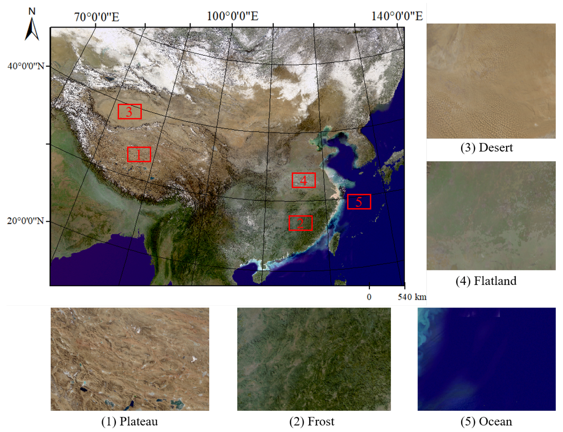
To better show the practicability of our method, the region we selected is the entire Chinese region, as shown in Figure 1, and the resolution of the image is 250 m. The dataset contains different types of features such as deserts, grasslands, oceans, etc. We only use the visible light band for training and testing. In our work, we downloaded several pieces of FY-3D satellites images, and these data cover different landcovers. Our dataset is marked and verified individually by an independent and skilled group from the China Meteorological Administration. A pixel is marked as cloud if more than half the members agree. According to statistics, most of the ambiguous pixels are cloud boundaries and thin cloud regions, and these pixels account for no more than of all pixels.

Figure 1.
Location and true-color combination 250 m FY-3D data (R, G, B) of the study area. The region contains many kinds of landcover, including oceans, deserts, forests, plateau, and others.
2.1. Preprocessing of Experimental Data
The spatial resolution of the FY-3D remote-sensing imagery used in the experiment is 250 m. This work uses the consensus of several experts to label remote-sensing images to ensure the correct classification of clouds. We choose the entire Chinese region for research because this area contains various landcovers, including oceans, deserts, forests, grasslands, and others. At the same time, the diverse climate in the region leads to clouds with different shapes, all of which increase the difficulty of detection. After data preprocessing (such as cropping), the data contains 24,659 × 14,165 pixels. The remote-sensing image is cropped by a sliding window in 512-pixel steps. In addition, we used random left and right flips and up and down flips for some data during training, and added “salt and pepper noise” to increase the size of the dataset and avoid overfitting. There will be a large number of whole images that are all clouds after cropping. Such a large number of full cloud and fog samples will make the model difficult to train and reduce the accuracy of detection. Therefore, we include images with different cloud coverage in the training set and test set, so that the network can be well trained.
After our careful selection, the dataset has 6959 images, of which (1392 images) are used as the test set to verify the proposed model, and (5567 images) are used as the training set. There are 669, 623, 879 cloud pixels and 789, 731, 769 clear pixels in the training set, which account for 45.88% and 54.12% of the whole training pixels. On the other hand, the test set contains 146, 582, 117 cloud pixels and 218, 322, 331 clear pixels, which occupy 40.17% and 59.83% of the entire testing pixels.
The distribution of image patches with different cloud coverage ratios are roughly similar in the two datasets. The details of the image patch distribution are summarized in Table 1.

Table 1.
Image distribution of cloud coverage in training and test datasets.
2.2. Our Method
To meet the needs of subsequent experiments, we divided the downloaded satellite images into a training set and a test set. The training set contains 5567 images, and the test set contains 1392 images. Coverage of clouds and the types of surface objects are fully considered when dividing the dataset. Most of the images contain cloud and free areas. Cloud regions include small, medium, and large clouds; the underlying surface environment includes vegetation, agricultural, water and snow.
Deep learning has been widely used in various tasks of remote-sensing image processing. Convolutional neural networks are used in tasks such as object detection, semantic segmentation, saliency detection, because of its excellent fitting ability. The Feature Pyramid Network [44] is adopted in many tasks because of its ability to synthesize features from different scales. Large-scale features can ensure that details are mined, while small-scale features can make the global information easily extracted. Non-Local Block [45] is introduced to build the connection between the global information and the local information, which allows for a better characterization and exploitation of clouds by combining rich global and local information. These two ideas are both important to the task of cloud detection, so we combine these two blocks to exploit long-range correlation information to detect cloud. The network structure is shown in Figure 2.
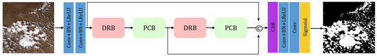
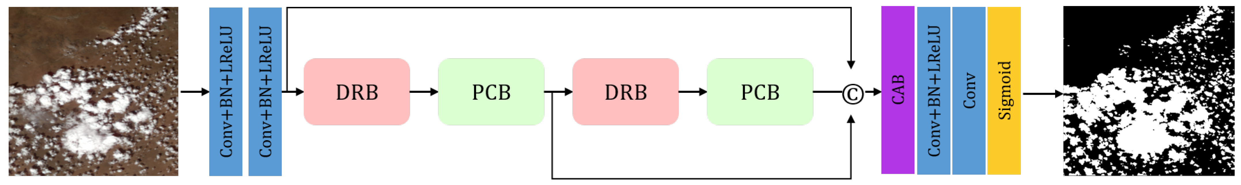
Figure 2.
The architecture of the proposed Pyramid Contextual Network for cloud detection contains Dilated Residual Blocks (DRB), Pyramid Contextual Blocks (PCB), and Channel Attention Block (CAB). The DRB includes dilated convolution and residual connection to acquire a wider receptive field. The PCB is designed for grasping global contextual information. The CAB is used for choosing the best channel to make the cloud mask. The network takes a cloud image as input and outputs the cloud mask.
2.2.1. Dilated Residual Block
In cloud detection, because of the existence of large clouds, we should pay more attention to global information when extracting features. Dilated convolution [46] is adopted because of its excellent ability to extract features. Dilated convolution is embedded holes in the regular convolution which increases the receptive field. It has one more hyper-parameter called dilation rate, which refers to the number of kernel intervals, e.g., the dilated rate of regular convolution is 1.
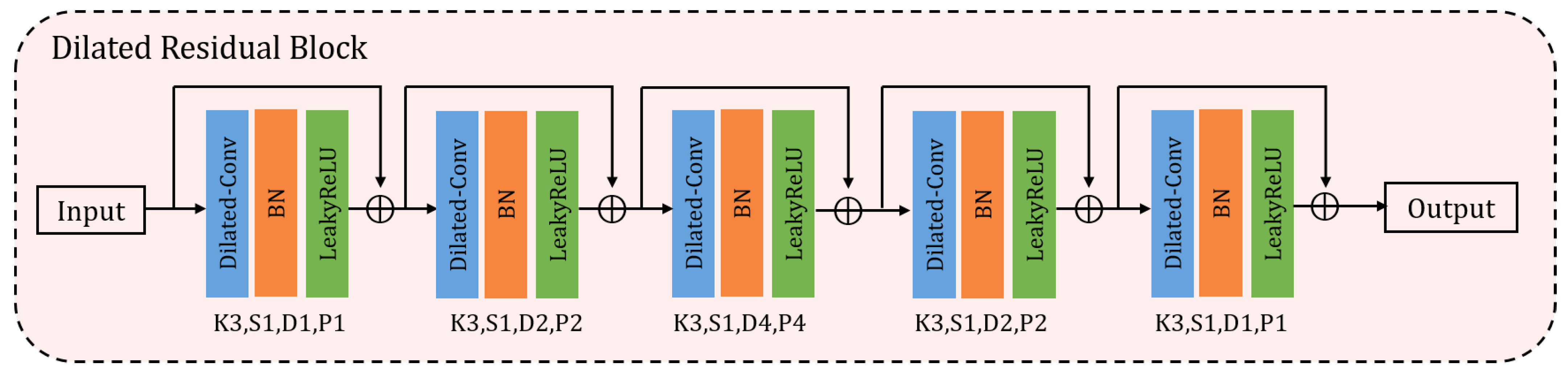
The architecture of DRB is shown in Figure 3. First, the input feature map is fed into dilated convolution and then normalizes the feature values through the Batch Normalization layer. Finally, it is activated by LeakyReLU layer. Our DRB contains five blocks; each block is composed of Dilated Conv-BN-LeakyReLU. All the size of convolution kernel is , and the dilatation ratios are 1, 2, 4, 2, 1; the padding sizes are also 1, 2, 4, 2, 1 to ensure the size of feature maps remains unchanged, the details are shown in Table 2. To preserve the information of the first group, we also add the residual connection to ensure that there is no loss of information from the beginning layers. The number of blocks and the dilated rates will be detailed in Section 3.3.2.
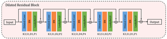
Figure 3.
Architecture of Dilated Residual Block. The input feature is fed into DRB block and go through five Dilated Conv-BN-LeakyReLU groups. To preserve the information of the input feature, we add the residual connection to ensure that there is no loss of information from the beginning layers. K, S, D, P mean kernel size, stride, dilated rate and padding size, respectively.
Table 2.
The structure of Dilated Residual Block (input size = ).
2.2.2. Pyramid Contextual Block
After the image is processed by the initial convolution and DRB, we obtain feature map , H, W, C representing height, weight and channel, respectively. Before we introduce pyramid contextual block, we first review non-local block [45], specified as follows:
means the feature map processed by non-local block. is attention map, means similarity between i pixel and j pixel of the original feature maps. is feature map embedded to N-dimension. is a diagonal matrix for normalization purposes. is a transforming function to recover the channel of feature map to C as equal as the original feature F. In this way, the feature map can be globally enhanced by the whole position of the feature map and the correlation between all pixels. Additionally, in [45], it can be constructed by taking the linear embedded Gaussian kernel to compute the feature map , and the linear function to calculate :
is convolutional operation with parameters of . When generating , we use and as the convolution kernels. and have the same size. To compress the features in channel dimension and reduce the amount of calculation, all convolutions use kernel size of [45].
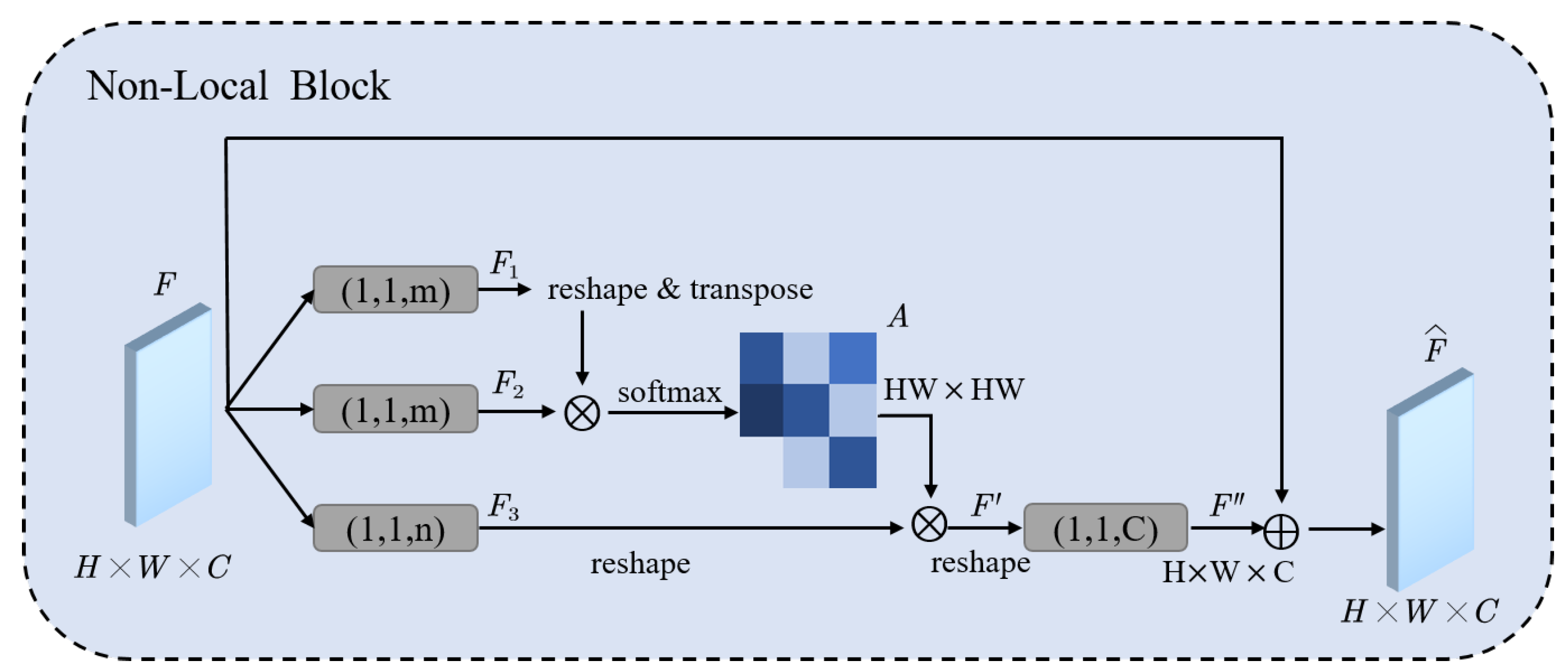
As we can see in Figure 4, feature map is fed to three convolution layers to generate , , and then reshape them to , , . We obtain the attention map A by SoftMax the result of multiplying and , attention map indicates the similarity of each pixel. is calculated by multiplying the attention map and , then recover the channel of by feeding it to a convolution layer. Finally, we obtain the enhanced feature map by adding and F.
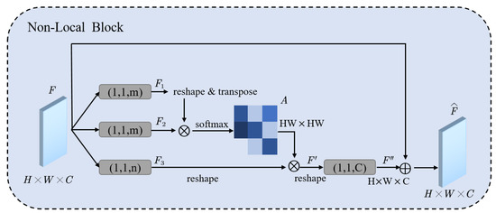
Figure 4.
The architecture of non-local block [45]. “⨂” denotes matrix multiplication, and “⨁” denotes the element-wise sum. The SoftMax operation is performed on each row. A is the attention map which can capture long-range dependencies. The gray boxes denote convolutions, (k, s, f) mean kernel size k, stride s and number of filters f.
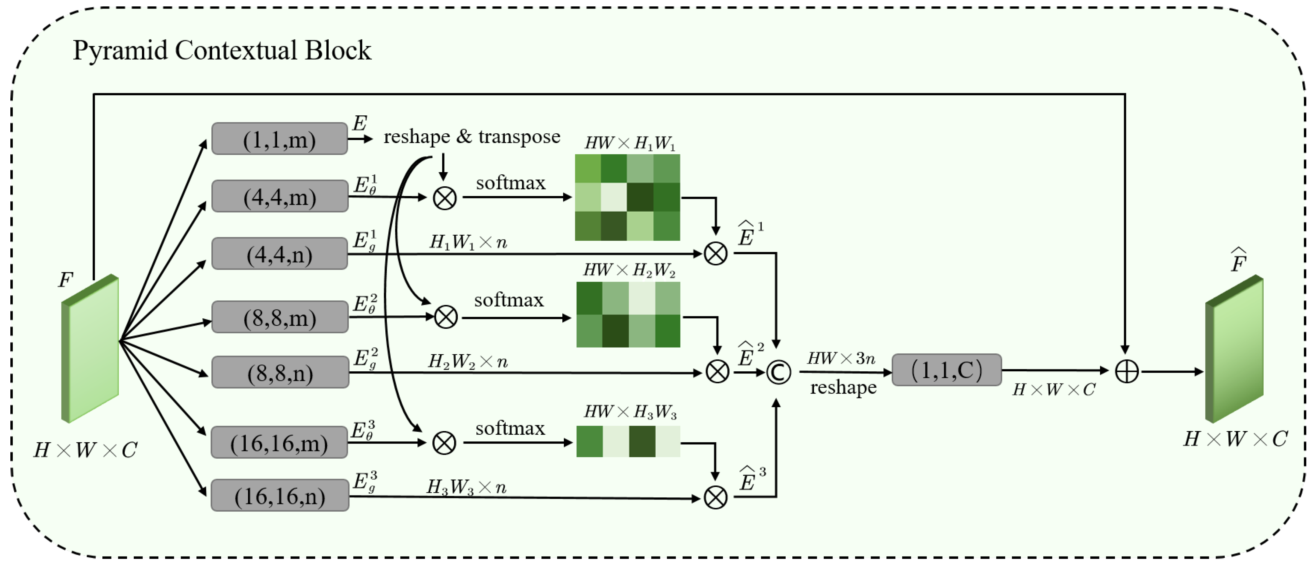
Please note that the non-local block is a brilliant attention mechanism, but there is a major trade-off. The attention map is generated by two feature maps, whose sizes are . The computational costs and memory consumptions of non-local block arise quadratically as the spatial size of input feature map increases. To solve this problem and to obtain long-range correlation of the whole image, we use multi-scale features and different sizes of convolution kernels to reduce the parameters. From the structure of our block in Figure 5, we can see that our block contains three branches, E is the result of the input feature map to convolution, and are the feature maps obtained by convolution layers. The size of and becomes , the sizes of and , and are , respectively, which greatly reduces the cost of computation, such that the global information can be grasped by the larger kernel sizes and the larger strides.
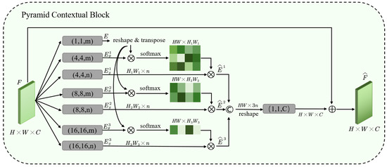
Figure 5.
The architecture of our Pyramid Contextual Block. “⨂” denotes matrix multiplication, and “⨁” denotes element-wise sum. The SoftMax operation is performed on each row. Compared with non-local block, we use multi-scale features and different sizes of convolution kernels to reduce the parameters and obtain long-range correlation of the whole image. , and are the enhanced features generated by multi-scale attention maps. is the output feature of PCB. The gray boxes denote convolutional layers, (k, s, f) mean kernel size k, stride s and number of filters f.
Then, the feature map of each of our branches can be expressed by the following equation:
Finally, we concatenate the features from all the branches and feed the result to convolution to change channels of the result to be consistent with the input feature map, and add the input feature to obtain the .
is a diagonal matrix for normalization purposes, is result of the branch. is the final convolution layer.
Under the premise of reducing the amount of calculation, PCB fully uses the information from multi-scale features to capture clouds with different sizes. Moreover, it can exploit the long-range connection between each pixel. In cloud detection, we should expand the receptive field to the entire image because the cloud can exist anywhere and have any size.
2.2.3. Channel Attention Block
After DRB and PCB have processed the feature map, it has used the contextual information in the image to perceive the area where clouds and fog exist. As shown in Figure 2, the feature map passes through the last PCB and concatenates the features of the previous layer together. There will inevitably be some redundant feature layers. We used SE Block [42] to select the appropriate channels that adaptively recalibrates channel-wise feature responses by explicitly modelling interdependencies between channels.
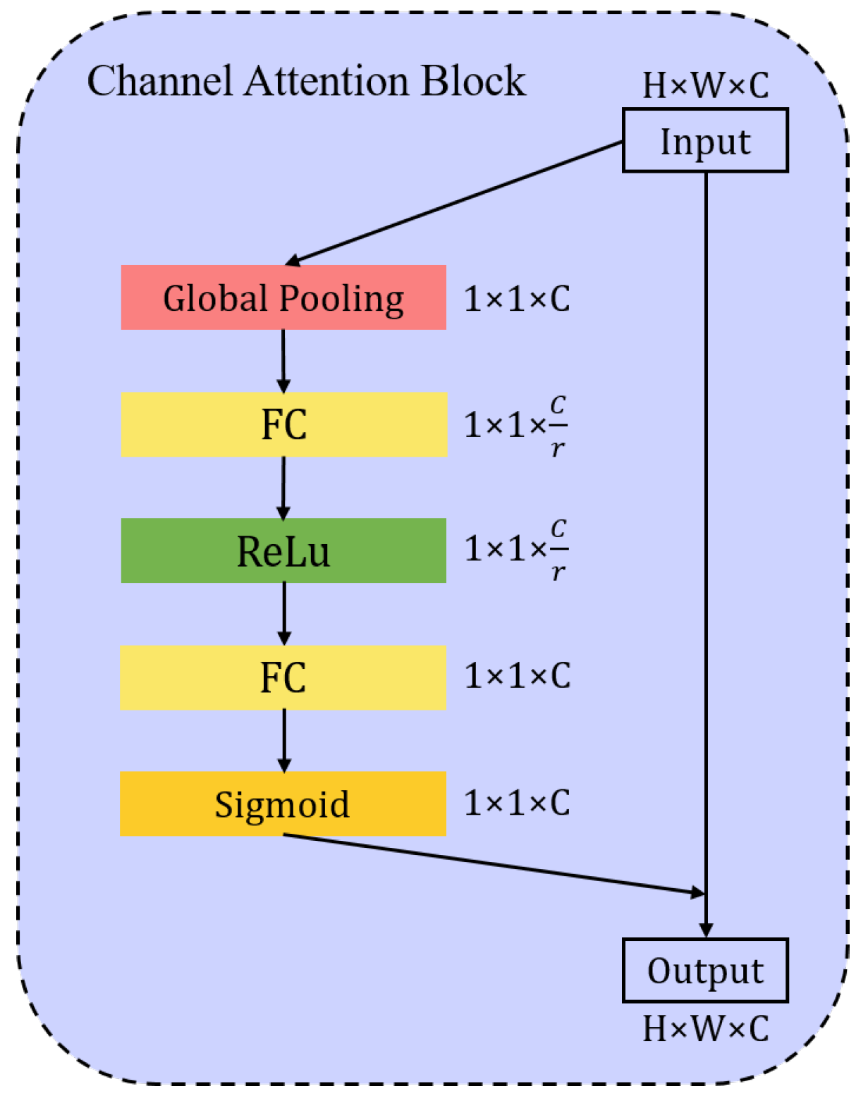
The input features are first passed through squeeze and resample operations (Global Pooling, FC, ReLU, FC shown in Figure 6), which aggregates the feature maps across spatial dimensions to produce a channel descriptor. This descriptor embeds the global distribution of channel-wise feature responses, enabling information from the global receptive field of the network to be fully used. This is followed by an excitation operation (Sigmoid shown in Figure 6), in which sample-specific activations, learned for each channel by a self-gating mechanism based on channel dependence, govern the excitation of each channel. The feature maps are then reweighted to generate the output which can be fed directly into subsequent layers.

Figure 6.
The architecture of Channel Attention Block. The feature map obtains a channel descriptor of after squeeze and resampling operations. Then, it is activated by a self-gating mechanism based on channel dependence. The feature maps are reweighted to generate the output which can be fed directly into subsequent layers.
In Figure 6, sigmoid is set as the second activation function to obtain the normalized channel weights because it can remap any real number to (0, 1) and keep the original information in channel dimension [42].
2.2.4. Pyramid Contextual Network
Our proposed network as shown in Figure 2. The input is processed by two convolution layers to calculate the feature map with ,
where I is the input image and is the initial convolution layers. Subsequently, we send to our enhanced block, where each block contains DRB and PCB, we assume is the output of the block,
and is PCB and DRB, and is the weight of them. After the same processing twice, we concatenate the final output feature map of each module together and output it after processing by the output convolutional layer.
2.2.5. Loss Function Optimization
Cloud detection is a binary classification problem, so we use cross-entropy as our loss function to obtain the cloud mask with high accuracy,
where is the classification result generated by our network, is the true cloud mask.
3. Results and Discussion
3.1. Implementation Details
3.1.1. Input Data
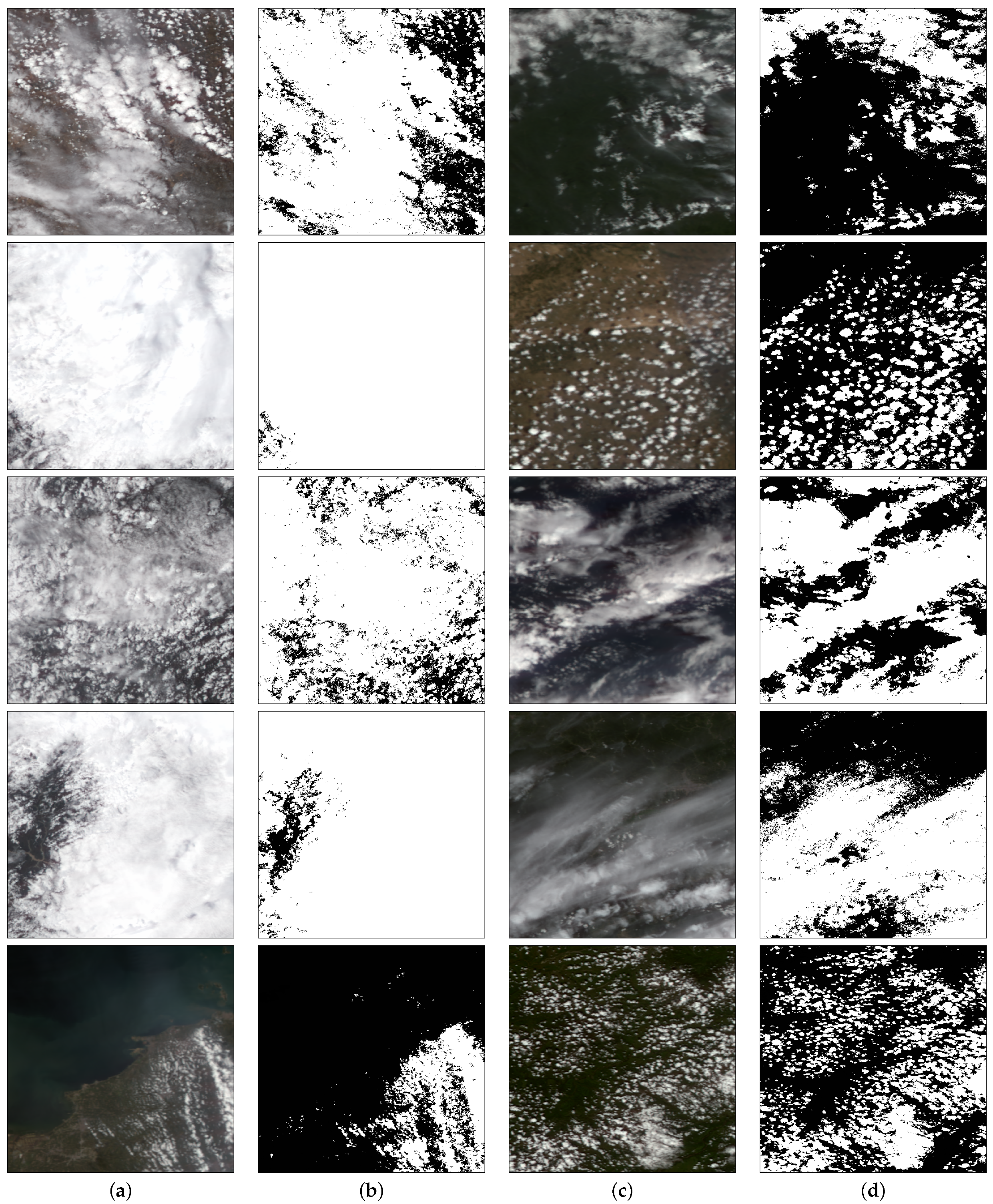
All the prepared sample data, including three original bands, namely R, G, B and the corresponding ground truth labels were used as inputs to the Pyramid Contextual Net. The input data used by the deep neural network are shown in Figure 7.
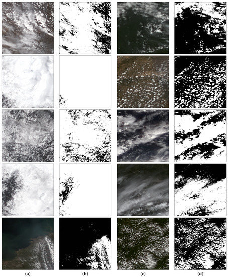
Figure 7.
Some samples in our dataset. Our dataset contains different landcovers, including oceans, deserts, forests, grasslands, and others. (a,c) Cloud Images; (b,d) Masks.
3.1.2. Set of Hyperparameters
Due to the complexity of our network structure, we need to initialize the network parameters. The weight of the convolution operation is initialized to a Gaussian distribution with a mean of 0 and a variance of 0.01, the bias is 0.1, and the weight of Batch Normalization is set to 0.1. To fit the network as quickly as possible, we use Adam optimizer [47] to optimize the network. The exponential decay rates for the first and second moment estimates are set to 0.9 and 0.999, respectively. The initial learning rate is set to 1 × 10⁻⁴, and reduced to half of the original number every 20 epochs, a total of 100 epochs, and the batch size is set to 1. All the output probabilities of each pixel from a Sigmoid classifier are translated to binary values with a threshold of 0.5 (0.5 as a default setting in a binary segmentation) [48].
3.2. Experimental Results
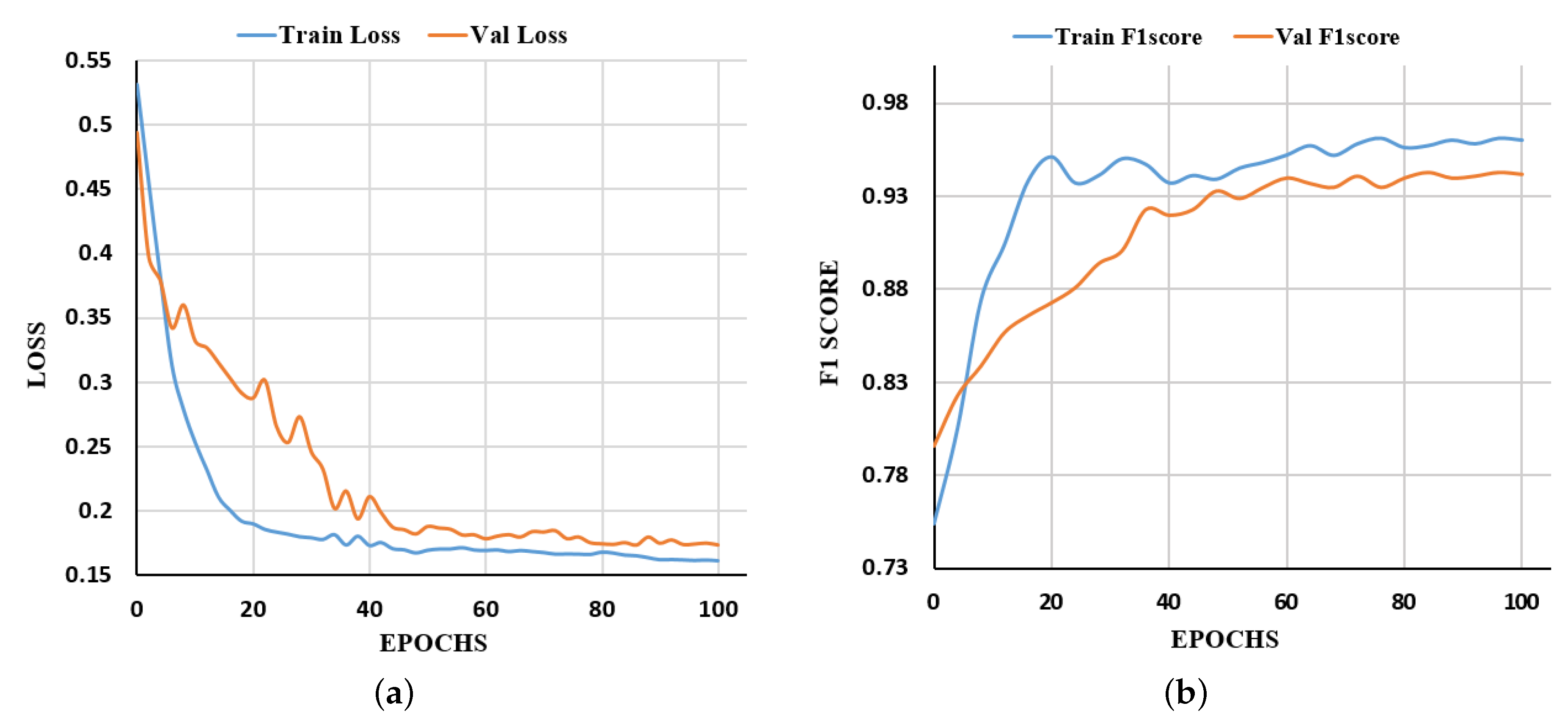
In this section, we compared our model with other state-of-the-art methods to verify the validity of our model. The training and testing environments are as follows: Our proposed model was implemented using the open-source Pytorch framework provided by Facebook in Python. Our platform is Ubuntu 20.04 with NVIDIA GTX 3090 GPU (24 GB). After 100 epochs, our model achieved state-of-the-art results on the dataset (Figure 8).
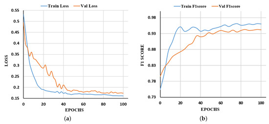
Figure 8.
Loss and F1 Score of PCNet for training and validating the datasets. (a) The training and validation loss change with the epochs on the datasets. (b) The training and validation F1 Score change with the epochs on the datasets.
3.2.1. Quantitative Analysis
In this section, we will compare the quantitative performance of our model. This work is compared with some new methods, including U-Net [49], UNet++ [50], UNet3+ [51], PSPNet [52] and DeepLabV3+ [53] to evaluate the effectiveness of the proposed PCNet in detecting cloud from remote-sensing images. The methods mentioned above are open-source and available on https://github.com/ (accessed on 15 February 2021). All methods have been trained and tested on the same dataset. The dataset has 6959 images, of which (1392 images) are used as the test set and (5567 images) are used as the training set. Compared with U-Net, UNet++ adds Dense Connections to re-use the feature maps. UNet3+ adds Full-scale Skip Connections to explore the full-scale ability of sufficient information and uses Full-scale Deep Supervision to constrain the intermediate features extracted by the network and improves the network’s capabilities. PSPNet is also listed as a comparison method. PSPNet uses the Pyramid pooling Module to collect hierarchical information to classify the pixels in the image better. Moreover, we also compare with DeepLabV3+. DeepLabV3+, as the best method in the DeepLab family, uses Atrous Spatial Pyramid Pooling to obtain a larger field of perception. In addition, the network is also improved an encoder–decoder structure to preserve feature information. To show the outstanding performance of our method, we compared with the current commonly used U-Net, UNet++, UNet3+, PSPNet and DeepLabV3+.
We used precision, recall, F1 Score and accuracy [36,38,54] to quantitatively evaluate the performance of our model in detecting clouds from remote-sensing images. These measurements are defined as follows:
where TP is true positive, TN is true negative, FP is false positive and FN is false negative. P and R are Precision and Recall, respectively. The accuracy assessment was performed as binary, all non-cloud features were combined into one feature. The results are shown in Table 3. The overall precision of our model reached , and the F1 score reached , which proved that our proposed method was excellent in detecting clouds from the remote-sensing imagery.
Table 3.
Quantitative comparison of cloud detection with Precision, Recall, F1 Score and Accuracy. The best results are marked in bold font.
The experimental results in Table 3 prove the better performance of our proposed method. The F1 Score of PCNet was 0.951, which is higher than the other four results generated by U-Net, UNet++, UNet3+, PSPNet and DeepLabV3+. Our approach considers accuracy while maintaining a high recall rate and a low missed detection rate. Thanks to pyramid contextual block, the network has a better detection accuracy for small isolated clouds in the image. Dilated Residual Block with dilated convolution and residual connection allows the model to retain information from different stages and have a larger receptive field. We will test the effectiveness of these two modules in ablation experiments.
3.2.2. Quality Analysis
After analyzing the quantitative results, we will compare our results with the other four results qualitatively. All these samples are typical and have varying degrees of complexity, involving oceans, deserts, forests, etc. Particular diagnoses for different features also include clouds with different morphological characteristics such as thin clouds and thick clouds.
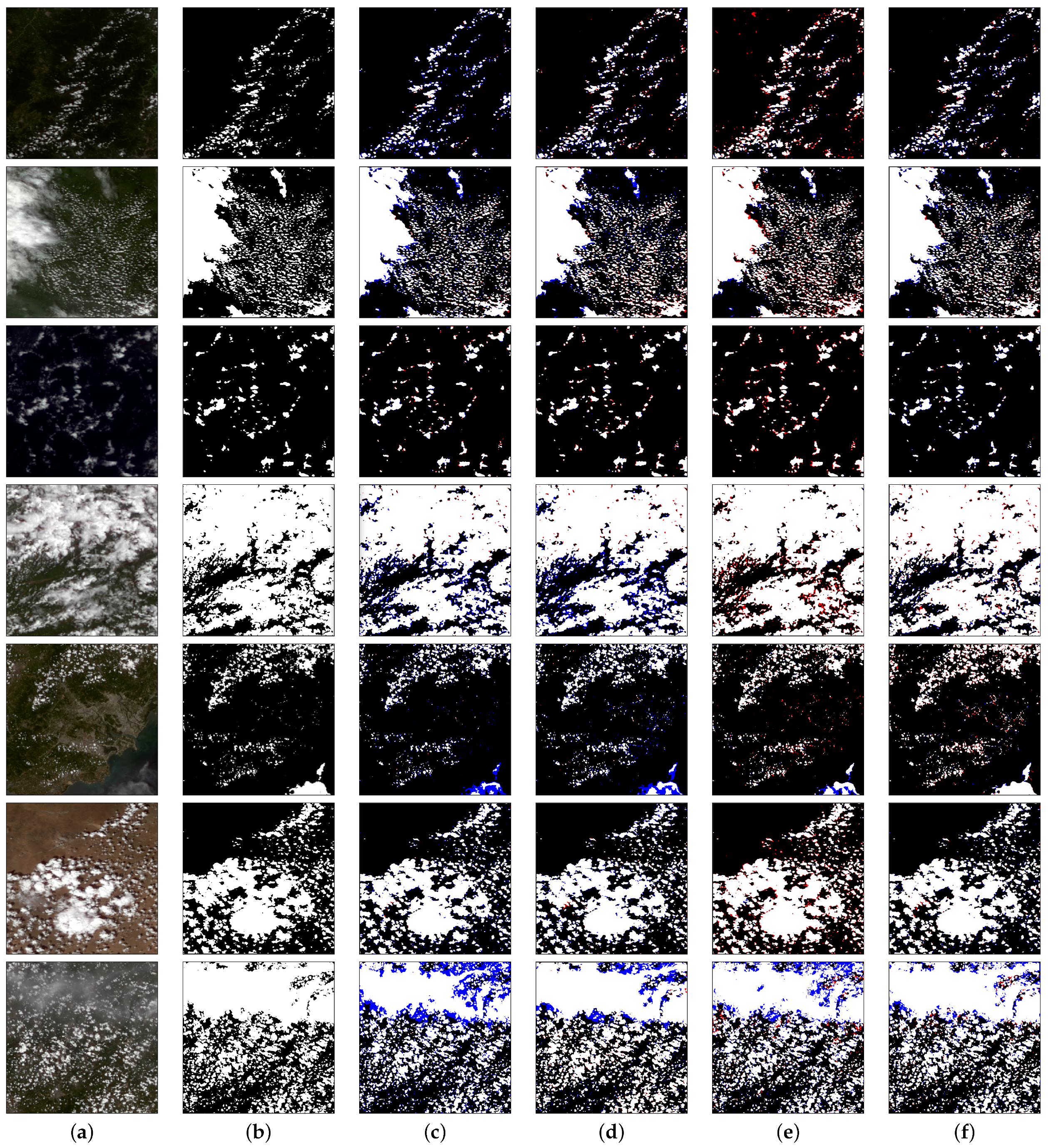
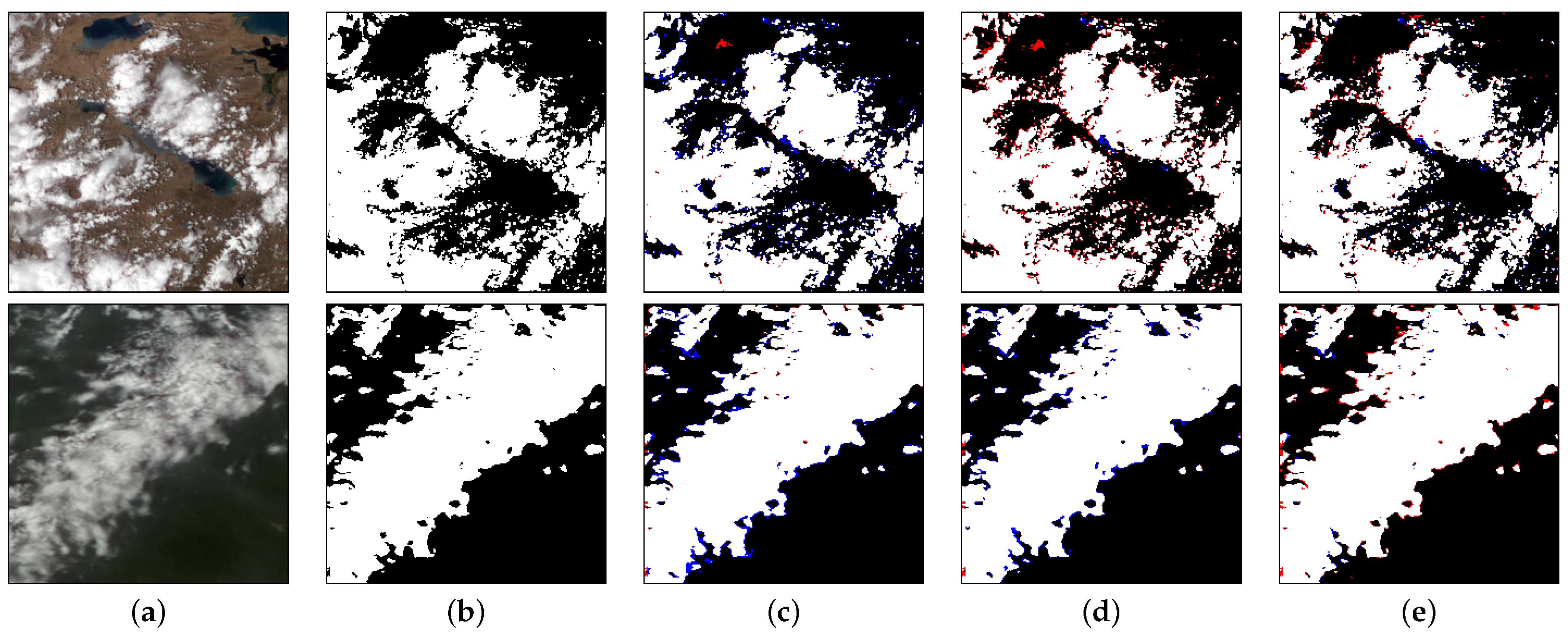
As can be seen from Table 3, due to the relatively low F1 Score of results generated by the U-Net and PSPNet, the predictions of these two methods will not be shown here; only UNet++, UNet3+, DeepLabV3+, and our model are compared. In Figure 9, the first line where UNet++ misses more detections may be because the method does not have strong constraints on the intermediate results and cannot perceive the global information of the image. Because DeepLabV3+ uses the ASPP module, it has a robust global perception of the image, but it treats some bright objects such as clouds, which causes more false detections. In addition to our method, the thin cloud area in the second row is more or less missed by the other three ways. The data in the 5th and 7th columns of Figure 9 show that the blue area in the DeepLabV3+ prediction result is much smaller than the other areas. This finding indicates that the perception ability of DeepLabV3+ model is more potent than UNet++ and UNet3+. The analysis of the network structure of the DeepLabV3+ shows that the model using dilated convolution and ASPP can effectively capture multi-scale information and improve the performance of cloud detection. We found that the blue area is significantly reduced in our results, but the red area has increased. This finding indicates that our method has vital data=fitting ability and can effectively mine the relationship between pixels to ensure precision while ensuring recall. The boundaries of some clouds are over-fitted, some non-cloud areas are classified as clouds because of the usage of PCB. Although some overfitting cases have been found, the overall performance of PCNet in cloud detection is still better than other pixel classification models.
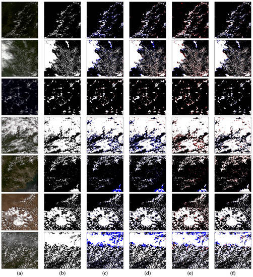
Figure 9.
The visualization of cloud detection. The first column (a) is the actual color of the FY-3D remote-sensing imagery; the second column (b) shows the corresponding ground truth; the third column (c) shows the results generated by UNet++ and the fourth column (d) shows the results generated by UNet3+; the fifth column (e) shows the prediction results of DeepLabV3+; the sixth column (f) shows the prediction results of our method. White, red, blue and black mean the TP, FP, FN and TN, respectively. (a) Input; (b) Ground Truth; (c) UNet++ [50]; (d) UNet3+ [51]; (e) DeepLabV3+ [53]; (f) Our.
3.2.3. Extended Experiments
- (a)
- Experiments in large-scale FY-3D true-color imagery
In the quantitative analysis and quality analysis mentioned earlier, the performance of our model has been intuitively reflected. To visually prove the superiority of PCNet, we selected some remote-sensing images of China in different periods to show the improved performance of our method. The size of the image is so large that it cannot be fed into the network, so we crop the image to a size of , and there is a overlap between each patch.
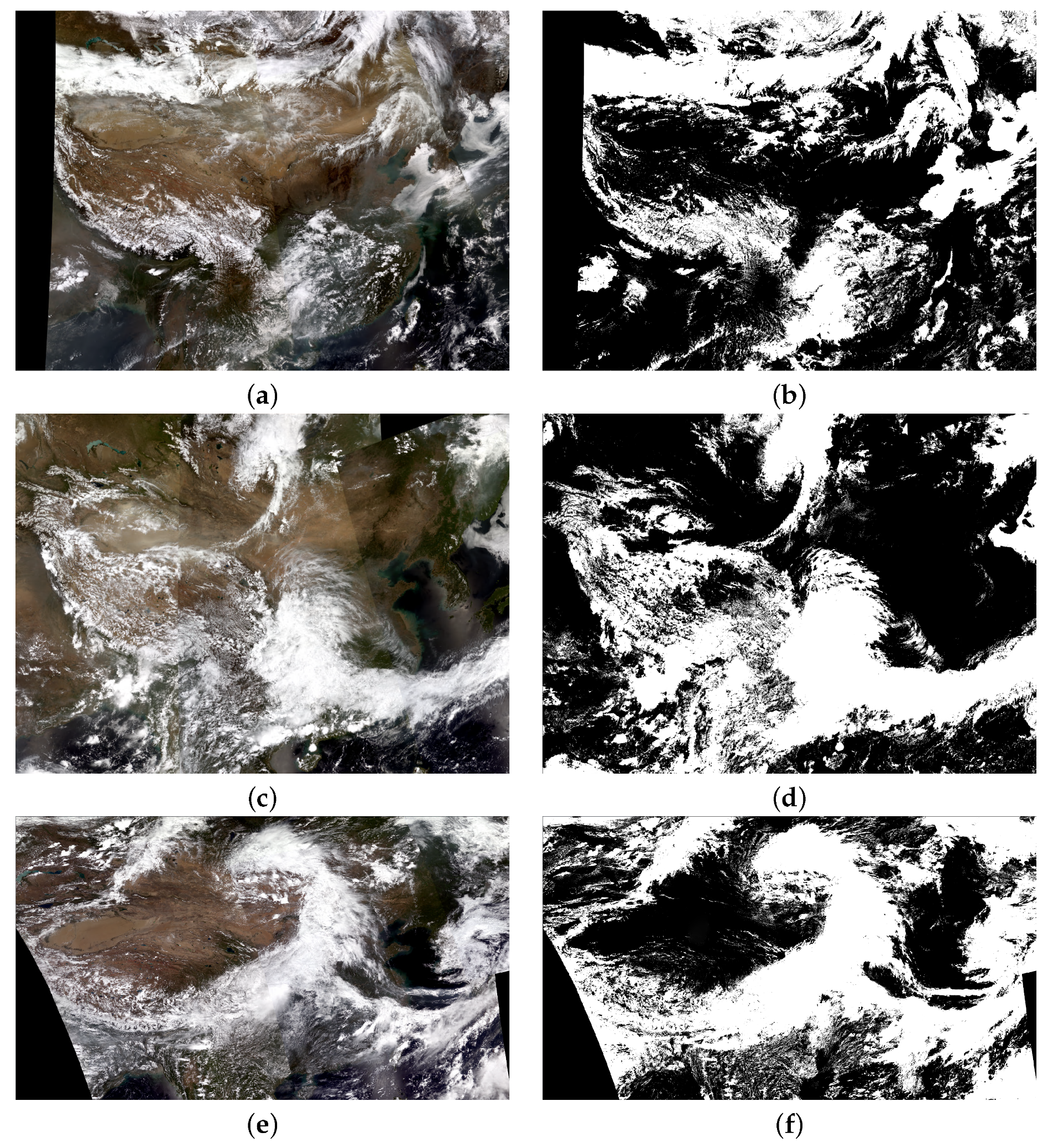
It can be seen from Figure 10 that the FY-3D images we used can cover the entire Chinese region. The sizes of the three images are as follows: 13,108 × 17,968, 13,108 × 17,968 and 14,165 × 24,659. Our method can also be better processed for large images. From the Figure 10b,d,f, the prediction results show that our method can detect both thin clouds, thick clouds and some isolated cloud clusters. Although we divide the whole picture into patches, there is no sense of division between blocks without any post-processing, which is enough to show the superiority of our method.

Figure 10.
The visualization of results for Chinese region. (a,c,e) True-color remote-sensing image of FY-3D MERSI 250 m. (b,d,f) The cloud masks generated by our method. (a) 1 April 2018, FY-3D MERSI-250 m actual color image of China. (b) The result generated by our method. (c) 1 June 2019, FY-3D MERSI-250 m actual color image of China. (d) The result generated by our method. (e) 3 July 2020, FY-3D MERSI-250 m actual color image of China. (f) The result generated by our method.
As the plateau area presented the left side of Figure 10, clouds and snow are hard to distinguish considering the confused visual features of the RGB images. According to the corresponding detection result by PCNet in the right side of Figure 10, snow was falsely detected as clouds.
- (b)
- Experiments in Landsat 8 true-color imagery
To show the applicability of our method, we added some experiments in Landsat 8 true-color imagery. We obtained the test images in https://earthexplorer.usgs.gov/ (accessed on 27 August 2021), and the serial numbers are LC08_L1TP_015032_20210614_20210622_01_T1 and LC08_L1TP_199026_20210420_20210430_01_T1, respectively.
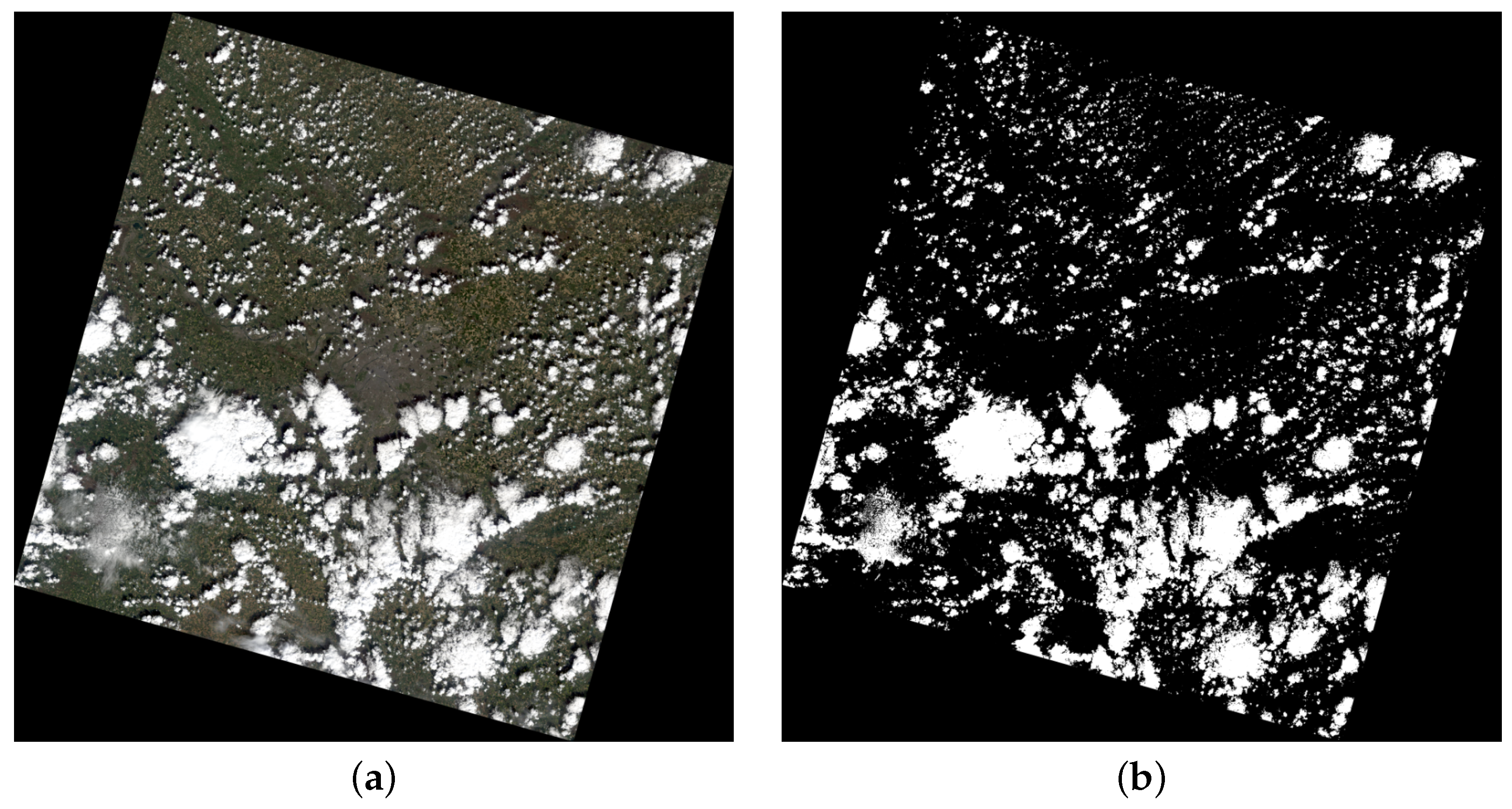
We employed the trained model using the FY-3D dataset to test in Landsat 8 true-color remote-sensing imagery. As we can see in Figure 11 and Figure 12, our method can acquire superior results for both isolated small clouds and clustered large clouds. However, some thin clouds are not detected because the model is not fine-tuned with Landsat 8 data.
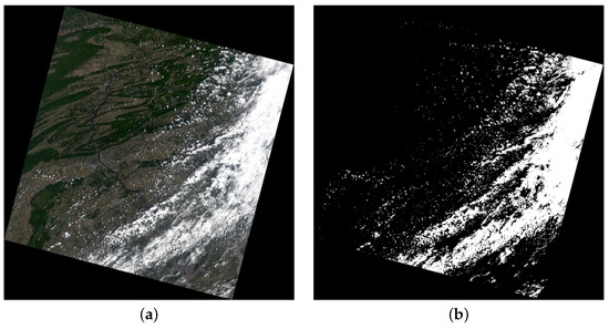
Figure 11.
The visualization of results for LC08_L1TP_015032_20210614_20210622_01_T1. (a) True-color imagery of Landsat 8. (b) The cloud mask generated by our method.
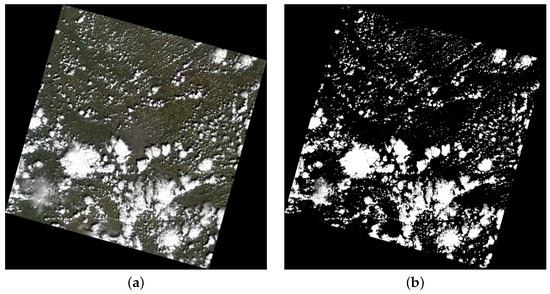
Figure 12.
The visualization of results for LC08_L1TP_199026_20210420_20210430_01_T1. (a) True-color imagery of Landsat 8. (b) The cloud mask generated by our method.
3.3. Ablation Study
To evaluate our network, we analyze the effect of each block and hyper-parameter used in our model. To make a fair comparison, all cases are trained, validated and tested, and conducted objective and fair investigations on the same dataset.
3.3.1. Effectiveness of Threshold for Sigmoid Classifier
The feature map is fed into a sigmoid classifier to generate the final result. As we can see in Table 4, we choose different thresholds to make comparisons, and they are set to 0.2, 0.3, 0.4, 0.5, 0.6, 0.7, 0.8.
Table 4.
The effectiveness of threshold for sigmoid classifier.
In Table 4, we can see that the values of precision rise and the values of recall fall as the number of thresholds increases. We choose as our threshold number because the value of F1 Score and accuracy is the highest. All the output probabilities of each pixel from a sigmoid classifier are translated to binary values with a threshold of 0.5 in our method. When the value of the output probabilities is greater than 0.5, we set it to 1 (cloud pixels). Otherwise, it is set to 0 (non-cloud pixels).
3.3.2. Effectiveness with Different Number of Blocks and Dilated Rates in DRB
In Figure 3, the input feature is fed into a DRB block and goes through five Dilated Conv-BN-LeakyReLU groups. To illustrate the effectiveness with different numbers of blocks and dilated rates in DRB, we choose different blocks and dilated rates to make comparisons. As shown in Table 5, when the number of blocks is four, we set the dilated rates as , , ; The dilated rates are set to , , , , and when the number of blocks is five. Furthermore, we compared the results which dilated rates are set to , , . Please note that dilated rates are equal to padding sizes in DRB.
Table 5.
This is effect analysis of the number of blocks and dilated rates.
When dilated rate = , it is regular convolution. In this case, the indicators are the worst when there are five blocks in DRB because the receptive fields are too small to consider the global information of the feature map. We can see that the precision is higher when dilated rate = than it when dilated rate = , and the recall is higher when dilated rate = than it when dilated rate = . It indicated that the network’s perception field is more extensive to correlate a larger area when dilated rate = , the bright objects may also be regarded as clouds, so the precision is low. When there are four Conv-BN-LeakyReLU groups in DRB, the network has difficulty fitting the distribution pattern of the dataset, which makes the results inferior to the results generated by five blocks. The results of the six blocks are the worst in Table 5, because the network has too many parameters to converge. To guarantee both precision and recall, we choose dilated rate = in our network.
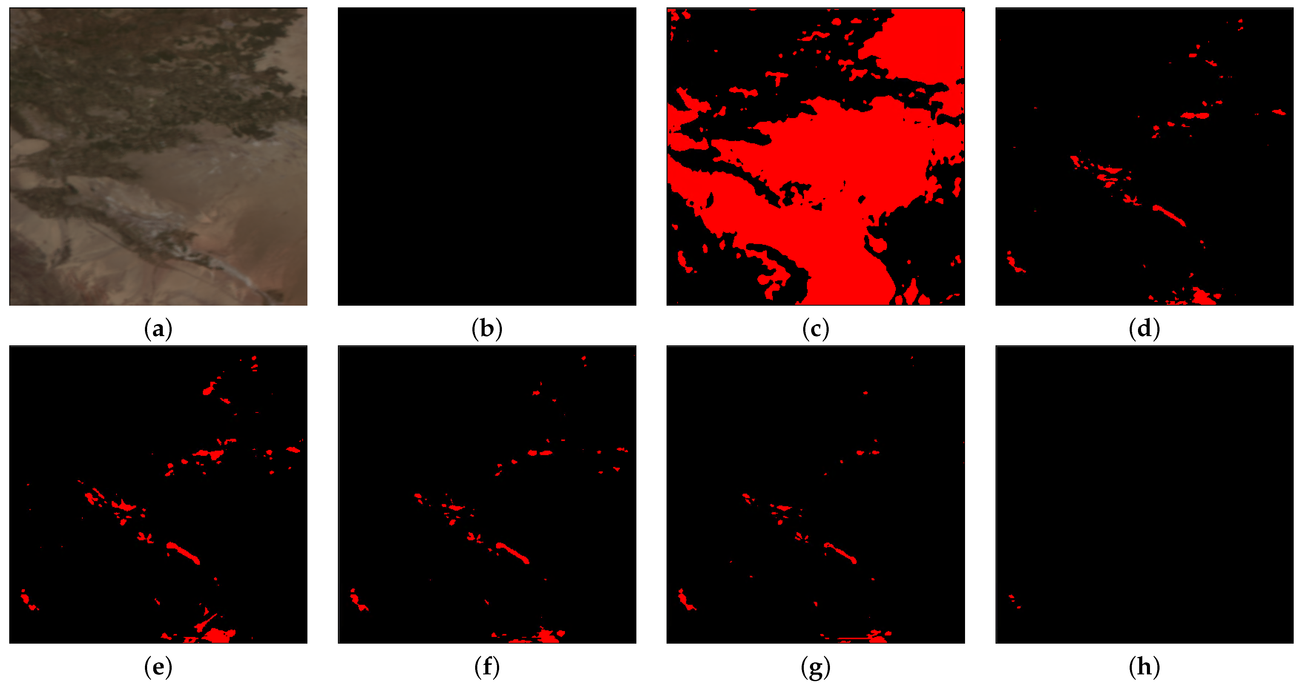
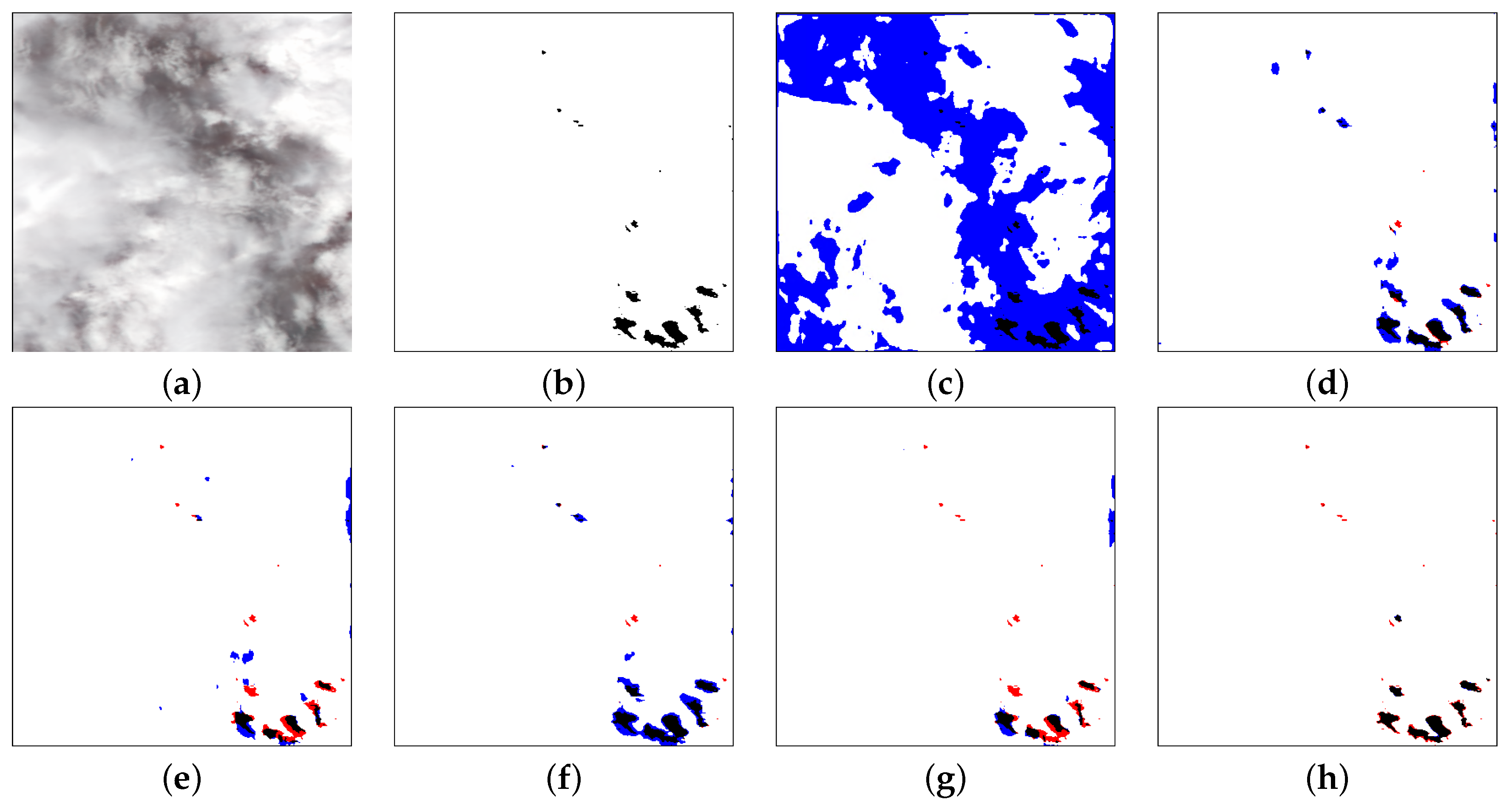
We only show the visualized results generated by the DRB, which has five Conv-BN-LeakyReLU blocks. In Figure 13, it is a regular convolution when dilated rate = , and the result of this case is the worst. When dilated rate = , Figure 14 shows that there are still more missed detections because the receptive field is relatively small compared with others; when dilated rate = , the receptive field is too large to classify the light pixels into clouds, resulting in more false detections. Figure 13 and Figure 14 show that the dilated rate adopted in our network can generate the most optimal prediction results.

Figure 13.
Cloud-detection results comparisons. From left to right are (a) input; (b) ground truth; (c) dilated rate = ; (d) dilated rate = ; (e) dilated rate = ; (f) dilated rate = ; (g) dilated rate = ; (h) dilated rate = . White, red, blue and black mean the TP, FP, FN and TN, respectively.

Figure 14.
Cloud-detection result comparisons. From left to right are (a) input; (b) ground truth; (c) dilated rate = ; (d) dilated rate = ; (e) dilated rate = ; (f) dilated rate = ; (g) dilated rate = ; (h) dilated rate = . White, red, blue and black mean the TP, FP, FN and TN, respectively.
3.3.3. Effectiveness with Different Number of Kernel Sizes in PCB
After determining the dilated rate as , since the effect of wider receptive field is obvious, we will compare the different kernel sizes in PCB, including , and .
As we can see in Table 6, the precision is the highest when kernel sizes = [2, 4, 8]. To take into account precision and recall, we choose as our kernel sizes. Additionally, there are some results shown in Figure 15. It can be seen from the first row that when strides = [2, 4, 8], the red part is small, which indicates the precision is higher as similar to the results shown in Table 6. Compared to the other two cases, our result has a higher recall.
Table 6.
The effectiveness of different numbers of kernel sizes in PCB for cloud detection.
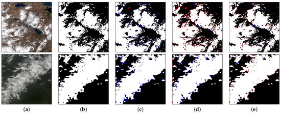
Figure 15.
Cloud-detection results comparisons. From left to right are (a) input; (b) ground truth; (c) strides = ; (d) strides = ; (e) strides = . White, red, blue and black mean the TP, FP, FN and TN, respectively.
3.3.4. Effectiveness of PCB Part
When the kernel sizes in PCB are determined, we will verify the necessity of PCB. We set two situations to confirm the robustness of PCB. Since the non-local block [45] is a widely used self-attention mechanism, we add one case that replaces PCB with Non-Local Block. “Only DRB” means replace the PCB with DRB, “NLB” means replace the PCB with Non-Local Block, “Params” refers to the number of variables that the model can automatically learn from the data. “MACs” refers to the number of multiply-accumulate operations and .
It can be seen from Table 7 that the Params of the module with only DRB have the smallest value. The Params and MACs of the module with PCB are similar to the module with non-local block but can achieve better results. There are also some results shown in Figure 16.
Table 7.
The effectiveness of PCB for cloud detection. The Params and MACs are calculated at the input size is .
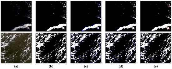
Figure 16.
Cloud-detection result comparisons. From left to right are (a) input; (b) ground truth; (c) replace the PCB with DRB; (d) replace the PCB with Non-Local Block; (e) Our method. White, red, blue and black mean the TP, FP, FN and TN, respectively.
3.3.5. Effectiveness of CAB Part
The feature map is concatenated and fed into the CAB after going through the DRB and PCB in Figure 2. Because the number of input feature channels is too large, there will inevitably be many useless feature maps. To alleviate this kind of problem, we added the CAB as our channel selector. “w/o CAB” means without CAB part, and “CAB” means with CAB part. As we can see from Table 8, if the CAB is not added, the result is slightly inferior to that which adds the CAB module. That is easy to say, during the training process, there is some redundant information in the feature maps.
Table 8.
The effectiveness of CAB for cloud detection.
In Table 8, we see that the quantitative result is slightly raised when adding the CAB, but the parameters of the network are increased. If a lighter model is required, we can choose the network without CAB.
4. Conclusions
Remote-sensing images from Landsat and MODIS are mostly investigated in cloud-detection research. The present research explores, for the first time, the effective cloud-detection method for the images from FY-3D. To this end, we generated a new dataset based on the FY-3D satellite and proposed a new cloud-detection model Pyramid Contextual Network. Based on the characteristics of clouds, a series of targeted modules are constructed: First, because of the small receptive field of regular convolutional blocks, we proposed DRB to expand the perception field of feature extraction. Second, we proposed PCB to explore the relationship between each pixel in the image for detecting isolated small clusters of thick clouds and thin clouds. Third, to reduce the redundancy of the feature maps, we used CAB to refine the feature maps.
The comparative experiments and adaptation to large-size remote-sensing imageries all proved the superiority of the proposed PCNet in cloud extraction. Moreover, in terms of the effectiveness of each module in the PCNet, a series of ablation experiments were conducted and evaluated by Precision, Recall, F1 Score, Params, etc. The proposed PCNet provides new insights into automatic cloud detection and is shown to outperform other typical deep-learning methods. Nevertheless, this work still has some unresolved problems. The proposed PCNet fails to distinguish clouds from snow at high latitudes since only RGB bands were used. In the future, more wavelengths will be used to support higher completeness and correctness of cloud detection. Additionally, we will focus on implementing a geoscience-knowledge-guided network and a network with extraordinary transferability. Geographical knowledge is barely integrated deeply to guide the network in detection of clouds and fog. For instance, thick clouds will not appear in desert areas as water vapor rarely exists. In terms of transferability, it is necessary that the PCNet or more networks in future to adapt to different satellite sensors and diverse geo-scenes.
Author Contributions
W.L. (Wangbin Li), K.S. and W.L. (Wenzhuo Li) designed the experiments; W.L. (Wangbin Li) conducted the experiments; X.H., J.W. and S.G. prepared the data; W.L. (Wangbin Li), K.S., Z.D. and W.L. (Wenzhuo Li) discussed the results. All authors contributed to the writing and revising of the manuscript. All authors have read and agreed to the published version of the manuscript.
Funding
This work was supported by the National Natural Science Foundation of China (No. 41801344, No. 41871249, No. 92038301, No. 91738301 and No. 41471354).
Institutional Review Board Statement
Not applicable.
Informed Consent Statement
Not applicable.
Data Availability Statement
All the data are available from the National Satellite Meteorological Center of China Meteorological Administration http://satellite.nsmc.org.cn/ (accessed on 10 July 2020).
Acknowledgments
We would like to thank the National Satellite Meteorological Center of China Meteorological Administration for providing satellite data. Moreover, we would like to thank the authors of these methods we compared, including U-Net, Unet++, Unet3+, PSPNet, Deeplabv3+. Our deepest gratitude goes to the reviewers and editors for their careful work and thoughtful suggestions that have helped improve this paper substantially. Code and data are available at https://github.com/WHUlwb/PCNet (accessed on 24 July 2021).
Conflicts of Interest
The authors declare no conflict of interest.
References
- Masó, J.; Serral, I.; Domingo-Marimon, C.; Zabala, A. Earth observations for sustainable development goals monitoring based on essential variables and driver-pressure-state-impact-response indicators. Int. J. Digit. Earth 2020, 13, 217–235. [Google Scholar] [CrossRef] [Green Version]
- Zhang, B.; Guo, Z.; Zhang, L.; Zhou, T.; Hayasaya, T. Cloud characteristics and radiation forcing in the global land monsoon region from multisource satellite data sets. Earth Space Sci. 2020, 7, e2019EA001027. [Google Scholar] [CrossRef] [Green Version]
- Irish, R.R.; Barker, J.L.; Goward, S.N.; Arvidson, T. Characterization of the Landsat-7 ETM+ automated cloud-cover assessment (ACCA) algorithm. Photogramm. Eng. Remote Sens. 2006, 72, 1179–1188. [Google Scholar] [CrossRef]
- Oreopoulos, L.; Wilson, M.J.; Várnai, T. Implementation on Landsat data of a simple cloud-mask algorithm developed for MODIS land bands. IEEE Geosci. Remote Sens. Lett. 2011, 8, 597–601. [Google Scholar] [CrossRef] [Green Version]
- Huang, C.; Thomas, N.; Goward, S.N.; Masek, J.G.; Zhu, Z.; Townshend, J.R.; Vogelmann, J.E. Automated masking of cloud and cloud shadow for forest change analysis using Landsat images. Int. J. Remote Sens. 2010, 31, 5449–5464. [Google Scholar] [CrossRef]
- Zhu, Z.; Woodcock, C.E. Object-based cloud and cloud shadow detection in Landsat imagery. Remote Sens. Environ. 2012, 118, 83–94. [Google Scholar] [CrossRef]
- Oishi, Y.; Ishida, H.; Nakamura, R. A new Landsat 8 cloud discrimination algorithm using thresholding tests. Int. J. Remote Sens. 2018, 39, 9113–9133. [Google Scholar] [CrossRef]
- Qiu, S.; He, B.; Zhu, Z.; Liao, Z.; Quan, X. Improving Fmask cloud and cloud shadow detection in mountainous area for Landsats 4–8 images. Remote Sens. Environ. 2017, 199, 107–119. [Google Scholar] [CrossRef]
- Zhang, R.; Sun, D.; Li, S.; Yu, Y. A stepwise cloud shadow detection approach combining geometry determination and SVM classification for MODIS data. Int. J. Remote Sens. 2013, 34, 211–226. [Google Scholar] [CrossRef]
- Li, P.; Dong, L.; Xiao, H.; Xu, M. A cloud image detection method based on SVM vector machine. Neurocomputing 2015, 169, 34–42. [Google Scholar] [CrossRef]
- Hu, X.; Wang, Y.; Shan, J. Automatic recognition of cloud images by using visual saliency features. IEEE Geosci. Remote Sens. Lett. 2015, 12, 1760–1764. [Google Scholar]
- Ma, C.; Chen, F.; Liu, J.; Duan, J. A new method of cloud detection based on cascaded AdaBoost. In Proceedings of the 8th International Symposium of the Digital Earth (ISDE8), Kuching, Malaysia, 26–29 August 2013; Volume 18, p. 012026. [Google Scholar]
- Zhang, Q.; Xiao, C. Cloud detection of RGB color aerial photographs by progressive refinement scheme. IEEE Trans. Geosci. Remote Sens. 2014, 52, 7264–7275. [Google Scholar] [CrossRef] [Green Version]
- Vivone, G.; Addesso, P.; Conte, R.; Longo, M.; Restaino, R. A class of cloud detection algorithms based on a MAP-MRF approach in space and time. IEEE Trans. Geosci. Remote Sens. 2013, 52, 5100–5115. [Google Scholar] [CrossRef]
- Tan, K.; Zhang, Y.; Tong, X. Cloud extraction from Chinese high resolution satellite imagery by probabilistic latent semantic analysis and object-based machine learning. Remote Sens. 2016, 8, 963. [Google Scholar] [CrossRef] [Green Version]
- Hollstein, A.; Segl, K.; Guanter, L.; Brell, M.; Enesco, M. Ready-to-use methods for the detection of clouds, cirrus, snow, shadow, water and clear sky pixels in Sentinel-2 MSI images. Remote Sens. 2016, 8, 666. [Google Scholar] [CrossRef] [Green Version]
- Shao, Z.; Deng, J.; Wang, L.; Fan, Y.; Sumari, N.S.; Cheng, Q. Fuzzy autoencode based cloud detection for remote sensing imagery. Remote Sens. 2017, 9, 311. [Google Scholar] [CrossRef] [Green Version]
- Joshi, P.P.; Wynne, R.H.; Thomas, V.A. Cloud detection algorithm using SVM with SWIR2 and tasseled cap applied to Landsat 8. Int. J. Appl. Earth Obs. Geoinf. 2019, 82, 101898. [Google Scholar] [CrossRef]
- Wei, J.; Huang, W.; Li, Z.; Sun, L.; Zhu, X.; Yuan, Q.; Liu, L.; Cribb, M. Cloud detection for Landsat imagery by combining the random forest and superpixels extracted via energy-driven sampling segmentation approaches. Remote Sens. Environ. 2020, 248, 112005. [Google Scholar] [CrossRef]
- Krizhevsky, A.; Sutskever, I.; Hinton, G.E. Imagenet classification with deep convolutional neural networks. Adv. Neural Inf. Process. Syst. 2012, 25, 1097–1105. [Google Scholar] [CrossRef]
- Liu, M.; Wang, X.; Zhou, A.; Fu, X.; Ma, Y.; Piao, C. UAV-YOLO: Small Object Detection on Unmanned Aerial Vehicle Perspective. Sensors 2020, 20, 2238. [Google Scholar] [CrossRef] [PubMed] [Green Version]
- Huang, Z.; Wang, J.; Fu, X.; Yu, T.; Guo, Y.; Wang, R. DC-SPP-YOLO: Dense connection and spatial pyramid pooling based YOLO for object detection. Inf. Sci. 2020, 522, 241–258. [Google Scholar] [CrossRef] [Green Version]
- Zhang, S.; Mu, X.; Kou, G.; Zhao, J. Object Detection Based on Efficient Multiscale Auto-Inference in Remote Sensing Images. IEEE Geosci. Remote Sens. Lett. 2020, 18, 1650–1654. [Google Scholar] [CrossRef]
- Xu, D.; Wu, Y. FE-YOLO: A Feature Enhancement Network for Remote Sensing Target Detection. Remote Sens. 2021, 13, 1311. [Google Scholar] [CrossRef]
- Zhang, C.; Harrison, P.A.; Pan, X.; Li, H.; Sargent, I.; Atkinson, P.M. Scale Sequence Joint Deep Learning (SS-JDL) for land use and land cover classification. Remote Sens. Environ. 2020, 237, 111593. [Google Scholar] [CrossRef]
- Kwan, C.; Ayhan, B.; Budavari, B.; Lu, Y.; Perez, D.; Li, J.; Bernabe, S.; Plaza, A. Deep learning for Land Cover Classification using only a few bands. Remote Sens. 2020, 12, 2000. [Google Scholar] [CrossRef]
- Liu, C.; Zeng, D.; Wu, H.; Wang, Y.; Jia, S.; Xin, L. Urban land cover classification of high-resolution aerial imagery using a relation-enhanced multiscale convolutional network. Remote Sens. 2020, 12, 311. [Google Scholar] [CrossRef] [Green Version]
- Pan, S.; Guan, H.; Chen, Y.; Yu, Y.; Gonçalves, W.N.; Junior, J.M.; Li, J. Land-cover classification of multispectral LiDAR data using CNN with optimized hyper-parameters. ISPRS J. Photogramm. Remote Sens. 2020, 166, 241–254. [Google Scholar] [CrossRef]
- Chen, J.; Yuan, Z.; Peng, J.; Chen, L.; Haozhe, H.; Zhu, J.; Liu, Y.; Li, H. DASNet: Dual attentive fully convolutional siamese networks for change detection of high resolution satellite images. IEEE J. Sel. Top. Appl. Earth Obs. Remote Sens. 2020, 14, 1194–1206. [Google Scholar] [CrossRef]
- Song, A.; Kim, Y.; Han, Y. Uncertainty analysis for object-based change detection in very high-resolution satellite images using deep learning network. Remote Sens. 2020, 12, 2345. [Google Scholar] [CrossRef]
- Saha, S.; Bovolo, F.; Bruzzone, L. Building change detection in VHR SAR images via unsupervised deep transcoding. IEEE Trans. Geosci. Remote Sens. 2020, 59, 1917–1929. [Google Scholar] [CrossRef]
- Zhang, C.; Yue, P.; Tapete, D.; Jiang, L.; Shangguan, B.; Huang, L.; Liu, G. A deeply supervised image fusion network for change detection in high resolution bi-temporal remote sensing images. ISPRS J. Photogramm. Remote Sens. 2020, 166, 183–200. [Google Scholar] [CrossRef]
- Mahajan, S.; Fataniya, B. Cloud detection methodologies: Variants and development—A review. Complex Intell. Syst. 2020, 6, 251–261. [Google Scholar] [CrossRef] [Green Version]
- Mateo-García, G.; Gómez-Chova, L.; Camps-Valls, G. Convolutional neural networks for multispectral image cloud masking. In Proceedings of the 2017 IEEE International Geoscience and Remote Sensing Symposium (IGARSS), Fort Worth, TX, USA, 23–28 July 2017; pp. 2255–2258. [Google Scholar]
- Li, Z.; Shen, H.; Cheng, Q.; Liu, Y.; You, S.; He, Z. Deep learning based cloud detection for medium and high resolution remote sensing images of different sensors. ISPRS J. Photogramm. Remote Sens. 2019, 150, 197–212. [Google Scholar] [CrossRef] [Green Version]
- Shao, Z.; Pan, Y.; Diao, C.; Cai, J. Cloud detection in remote sensing images based on multiscale features-convolutional neural network. IEEE Trans. Geosci. Remote Sens. 2019, 57, 4062–4076. [Google Scholar] [CrossRef]
- Liu, H.; Du, H.; Zeng, D.; Tian, Q. Cloud detection using super pixel classification and semantic segmentation. J. Comput. Sci. Technol. 2019, 34, 622–633. [Google Scholar] [CrossRef]
- Yang, J.; Guo, J.; Yue, H.; Liu, Z.; Hu, H.; Li, K. CDnet: CNN-based cloud detection for remote sensing imagery. IEEE Trans. Geosci. Remote Sens. 2019, 57, 6195–6211. [Google Scholar] [CrossRef]
- Luotamo, M.; Metsämäki, S.; Klami, A. Multiscale Cloud Detection in Remote Sensing Images Using a Dual Convolutional Neural Network. IEEE Trans. Geosci. Remote Sens. 2020, 59, 4972–4983. [Google Scholar] [CrossRef]
- Mwigereri, D.G.; Nderu, L.; Mwalili, T. A Multi-Feature Fusion Deep Convolutional Network Based on a Coarse-Fine Structure for Cloud Detection. 2020. Available online: http://ceur-ws.org/Vol-2689/paper9.pdf (accessed on 24 July 2021).
- Kanu, S.; Khoja, R.; Lal, S.; Raghavendra, B.; Asha, C. CloudX-net: A robust encoder-decoder architecture for cloud detection from satellite remote sensing images. Remote Sens. Appl. Soc. Environ. 2020, 20, 100417. [Google Scholar] [CrossRef]
- Hu, J.; Shen, L.; Sun, G. Squeeze-and-excitation networks. In Proceedings of the IEEE Conference on Computer Vision and Pattern Recognition, Salt Lake City, UT, USA, 18–23 June 2018; pp. 7132–7141. [Google Scholar]
- Yang, Z.; Zhang, P.; Gu, S.; Hu, X.; Tang, S.; Yang, L.; Xu, N.; Zhen, Z.; Wang, L.; Wu, Q.; et al. Capability of Fengyun-3D satellite in earth system observation. J. Meteorol. Res. 2019, 33, 1113–1130. [Google Scholar] [CrossRef]
- Lin, T.Y.; Dollár, P.; Girshick, R.; He, K.; Hariharan, B.; Belongie, S. Feature pyramid networks for object detection. In Proceedings of the IEEE Conference on Computer Vision and Pattern Recognition, Honolulu, HI, USA, 21–26 July 2017; pp. 2117–2125. [Google Scholar]
- Wang, X.; Girshick, R.; Gupta, A.; He, K. Non-local neural networks. In Proceedings of the IEEE Conference on Computer Vision and Pattern Recognition, Salt Lake City, UT, USA, 18–23 June 2018; pp. 7794–7803. [Google Scholar]
- Yu, F.; Koltun, V. Multi-scale context aggregation by dilated convolutions. arXiv 2015, arXiv:1511.07122. [Google Scholar]
- Kingma, D.P.; Ba, J. Adam: A method for stochastic optimization. arXiv 2014, arXiv:1412.6980. [Google Scholar]
- Wei, S.; Ji, S.; Lu, M. Toward automatic building footprint delineation from aerial images using cnn and regularization. IEEE Trans. Geosci. Remote Sens. 2019, 58, 2178–2189. [Google Scholar] [CrossRef]
- Ronneberger, O.; Fischer, P.; Brox, T. U-net: Convolutional networks for biomedical image segmentation. In Proceedings of the International Conference on Medical image computing and computer-assisted intervention, Munich, Germany, 5–9 October 2015; pp. 234–241. [Google Scholar]
- Zhou, Z.; Siddiquee, M.M.R.; Tajbakhsh, N.; Liang, J. Unet++: A nested u-net architecture for medical image segmentation. In Deep Learning in Medical Image Analysis and Multimodal Learning for Clinical Decision Support; Springer: Berlin/Heidelberg, Germany, 2018; pp. 3–11. [Google Scholar]
- Huang, H.; Lin, L.; Tong, R.; Hu, H.; Zhang, Q.; Iwamoto, Y.; Han, X.; Chen, Y.W.; Wu, J. Unet 3+: A full-scale connected unet for medical image segmentation. In Proceedings of the ICASSP 2020—2020 IEEE International Conference on Acoustics, Speech and Signal Processing (ICASSP), Barcelona, Spain, 4–8 May 2020; pp. 1055–1059. [Google Scholar]
- Zhao, H.; Shi, J.; Qi, X.; Wang, X.; Jia, J. Pyramid scene parsing network. In Proceedings of the IEEE Conference on Computer Vision and Pattern Recognition, Honolulu, HI, USA, 21–26 July 2017; pp. 2881–2890. [Google Scholar]
- Chen, L.C.; Zhu, Y.; Papandreou, G.; Schroff, F.; Adam, H. Encoder-decoder with atrous separable convolution for semantic image segmentation. In Proceedings of the European Conference on Computer Vision (ECCV), Munich, Germany, 8–14 September 2018; pp. 801–818. [Google Scholar]
- Long, J.; Shelhamer, E.; Darrell, T. Fully convolutional networks for semantic segmentation. In Proceedings of the IEEE Conference on Computer Vision and Pattern Recognition, Boston, MA, USA, 7–12 June 2015; pp. 3431–3440. [Google Scholar]


Publisher’s Note: MDPI stays neutral with regard to jurisdictional claims in published maps and institutional affiliations. |
© 2021 by the authors. Licensee MDPI, Basel, Switzerland. This article is an open access article distributed under the terms and conditions of the Creative Commons Attribution (CC BY) license (https://creativecommons.org/licenses/by/4.0/).