Abstract
This study examines the response of a cold-regions deltaic wetland ecosystem in northwestern Canada to two separate and differing seasonal wetting cycles. The goal of this paper was to examine the nature of reflected electromagnetic energy measured by earth observation (EO) satellites, and to assess whether seasonal wetland hydroperiod and episodic flooding events impact the information retrieved by the Sentinel-2 sensors. The year 2018 represents a year characterized by a large spring freshet and ice-jam flooding, while 2019 represents a year characterized more by summer open-water flooding. We applied the Modified Normalized Difference Wetness Index (MNDWI) to address the effects of the wetting cycles. The response of the vegetative cover was tracked using the fraction of the absorbed photosynthetically active radiation (fAPAR) and the Leaf Area Index (LAI). All three indices were viewed through the lens of cover classes as derived through a previously published study by the authors. The study provides a framework for designing longer-term studies where multiple intra- and inter-annual hydrological cycles can be accessed via EO data. Future studies will enable the examination of lag times inherent in the response to the various water sources applied to spectral response and incorporate this EO approach into a monitoring framework.
1. Introduction
Wetlands are important features in the landscape that provide numerous ecosystem services for people and animals, including storage of water and carbon, protecting and improving water quality, providing essential habitats and access to food, hunting and trapping areas, etc. [1]. These valuable functions are the result of the unique natural characteristics of wetlands; namely, that they form where the landscape is permeated or submerged by water on a permanent or temporary basis for a sufficient length of time to promote aquatic processes. With vegetation adapted to fluctuating water level/depth, wetlands are among the most productive ecosystems in the world, and the only ecosystem designated for conservation by an international convention [2]. Wetlands represent sensitive transition areas between terrestrial and aquatic ecosystems and thus, provide a critical indicator of environmental health [3]. Monitoring of the state of water extent and natural vegetation cover, along with associated processes such as green-up and senescence, provides us with insight as to the stresses being exerted on these sensitive areas as well as their state of health [4].
Earth observation (EO) data have long been applied to the monitoring of various landscapes and ecosystems. Toolboxes commonly applied to EO data contain a myriad of vegetation indices that have been used to assess the state of the vegetation cover [5,6]. Many of these indices are designed to use narrowly focused band-sets (known as narrow band indices, NBI) that are commonly available from hyperspectral imagers. These NBIs are inappropriate for use with the broad band sensors that are housed on most EO platforms. These sensors rely on broad-band indices that are less specific in their ability to characterize detailed vegetation properties, but rather, they provide insight into broader biomass-related issues [7]. With the advent of EO sensors with spectral band-sets that extend to the Shortwave Infrared (SWIR), we now have the opportunity to exploit a broader range of vegetation indices (VI). This allows us to be more specific in our characterization of the state of the vegetative cover and related ecological processes. One of the more recent additions to the portfolio of EO platforms is the Copernicus Sentinel-2 mission based on a constellation of two identical satellites in the same orbit, designed to collect wide-swath and high-resolution multispectral images [8].
The 13 band-set available through the Sentinel-2 constellation provides us with the possibility to extract a larger number of indices [9,10] that have been commonly available with, for example, the Landsat series of satellites. Three of the more intriguing indices are the modified normalized difference water index (MNDWI), fraction of the absorbed photosynthetically available radiation (fAPAR) and leaf area index (LAI). fAPAR is the amount of photosynthetically active radiation (400 to 700 nm wavelength range) that is used in photosynthesis. As such, it is commonly used as a surrogate for primary productivity [11,12,13] and is considered to be an indicator of plant or ecosystem health [13,14]. The leaf area index (LAI) is defined as the area of a leaf that is projected onto an underlying surface. LAI is related to the stomatal area and uptake of CO2, and as such, is tied to the fAPAR [15,16]; however, it is also seen as being responsive to longer-term biological processes. While there can be considerable discussion as to the efficacy, or indeed, relevance, of many globally defined or intended EO-derived metrics, these two Sentinel-2 derived metrics have been found to be consistent in describing the earth surface for the boreal mixed-wood ecosystem in which our study is based [17]. Discrepancies, however, were noted by previous work to be due to the “global” nature of the algorithm used to define the metrics. Putzenlechner et al. [17] found that fAPAR was linked to seasonal process patterns, but that these patterns were not as evident in the stands where conifers dominated.
The goal of this paper is to examine the nature of reflected electromagnetic energy as measured by EO satellites and to assess whether seasonal wetland hydroperiods, as well as episodic flooding events, impact the information retrieved by the Sentinel-2 sensors. To do this, we have derived three indices: MNDWI, fAPAR, and LAI. MNDWI will be used to track the wetting and drying of the surface through time. While the fAPAR is seen as being related to biological processes, and as such, is considered relatively instantaneous in its response, LAI is interpreted as being more of a delayed seasonal response to variations in growing conditions. Using these three indices, we examine the response of a deltaic wetland landscape within the context of the Peace–Athabasca Delta (PAD) located in northwestern Canada. The segmentation strategy detailed by Peters et al. [18] will be used to investigate a more nuanced examination of the response of the individual vegetation cover classes/ecosystems in this delta. Two years were chosen to focus upon as they represent a year with extensive spring ice-jam-related flooding in 2018 and a year characterized by notable summer open-water flooding in 2019.
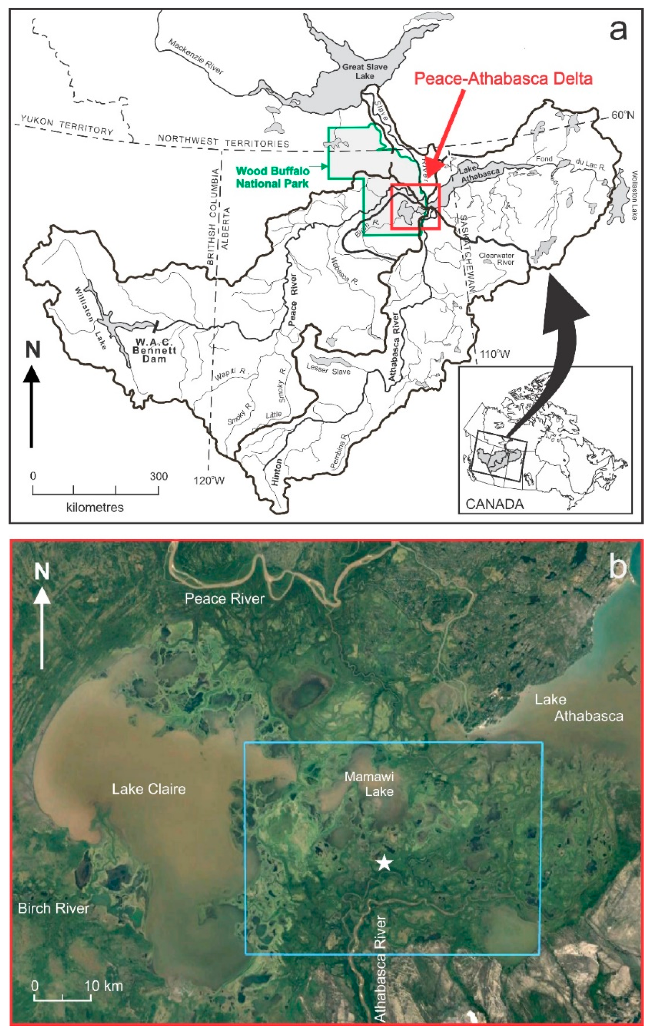
2. Study Area
The PAD formed at the convergence of the Peace, Athabasca and Birch River at the west end of Lake Athabasca in northern Alberta, Canada (Figure 1). The PAD is recognized by the Ramsar Convention as a wetland of international importance. Approximately 80% lies within the Wood Buffalo National Park, which is a UNESCO World Heritage Site. In addition to extensive deltaic floodplain areas (Peace ~1680 km2; Athabasca Delta ~1970 km2; Birch Delta ~170 km2), the PAD complex (~6000 km2) encloses several large interconnected lakes.
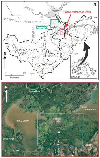
The river–lake–delta system drains Cordilleran and Boreal areas of approximately 600,000 km2 flowing northwards towards the Slave River. During high water events on the lower Peace River resulting from ice jams and high flows, drainage may reverse southward into the central lakes, and in extreme events, via overland pathways due to small elevational gradients [19,20]. The Peace River has been regulated since 1968 by a number of dams, which control the headwater runoff for the generation of hydroelectricity, leading to important changes to the flow regime near and within the delta, which were partially remediated with the building of weirs on outflow channels [19,20,21]. The Athabasca River mainstem is unregulated, with <5% of the natural flow allocated for agriculture, municipal and industrial water uses and has, thus, retained a near natural hydrological regime [22,23]. Oil sanding mining (open pit and in situ) is occurring in tributaries of the Lower Athabasca River, just upstream of the PAD, where landscape alterations and small amounts of water are abstracted from the mainstem for processing of bitumen [23,24].
The PAD contains >1000 inland wetland and lake basins with varying degrees of connectivity to the main flow system: open drainage, restricted and isolated basins [25,26]. The latter two classes are perched above and separated from the main flow system. Other than areas with significant local runoff input (e.g., Shield areas in northeast area of the PAD), restricted and isolated basins require periodic replenishment of water via overland flow routes activated during spring breakup ice jams or summer high flows to offset loses of water in between inundation events mainly through potential evapotranspiration. Potential evapotranspiration rates are, on average, greater (~10 cm) than local precipitation [27,28]. The generally prevailing semi-arid climate dominated by evapotranspiration rates, therefore, strongly influences surface water extents and depths in this area, with periodic flooding and water drawdown cycle resulting in a spatiotemporally variable wetland landscape, but highly productive ecosystem [29].
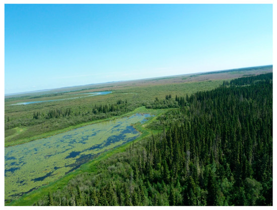
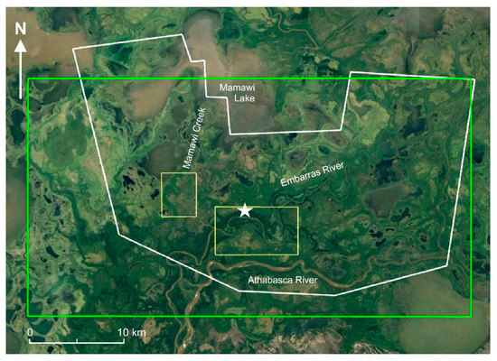
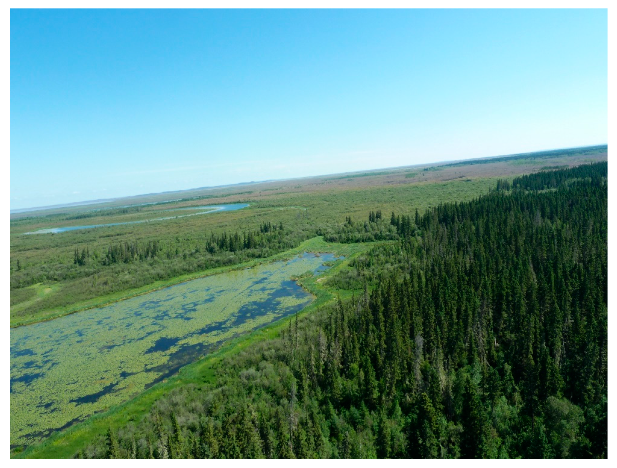
The PAD has been recognized as a primary habitat for a large range of insects, birds and mammals [29,30,31]. The vegetation cover, as reported on by Timoney [30], is affected by topography, frequency of flooding and depth to the groundwater table. Vegetation classes are generally organized along an elevation and moisture gradient: from forests (balsam poplar, white spruce) at the highest elevations, followed by thickets and savannahs (willows, grasses), marshes and meadows (sedges, grasses, rushes, cattails and reeds), and aquatic communities at the lowest elevations (algae-diatoms, bladderwort-duckweed-coontail, pond-lily) [29]. An example of such vegetation cover gradient and wetland channel complexes in the study area of interest within the Athabasca Delta are shown in Figure 2 and Figure 3.
3. Data and Processing
Sentinel-2 A and B data were obtained for the years 2018 and 2019. From the available image archive, largely cloud-free scenes spanning the growing seasons, and with relatively close calendar date correspondence between the years, were selected for analyses. As such, we acquired images during the open-water season from May, July, August, and September for both years (Table 1). Level 1c processed data, which provided orthorectified TOA (top-of-atmosphere) reflectance data, were employed.

Table 1.
Earth observation acquisition dates.
3.1. Ecosystem Structure
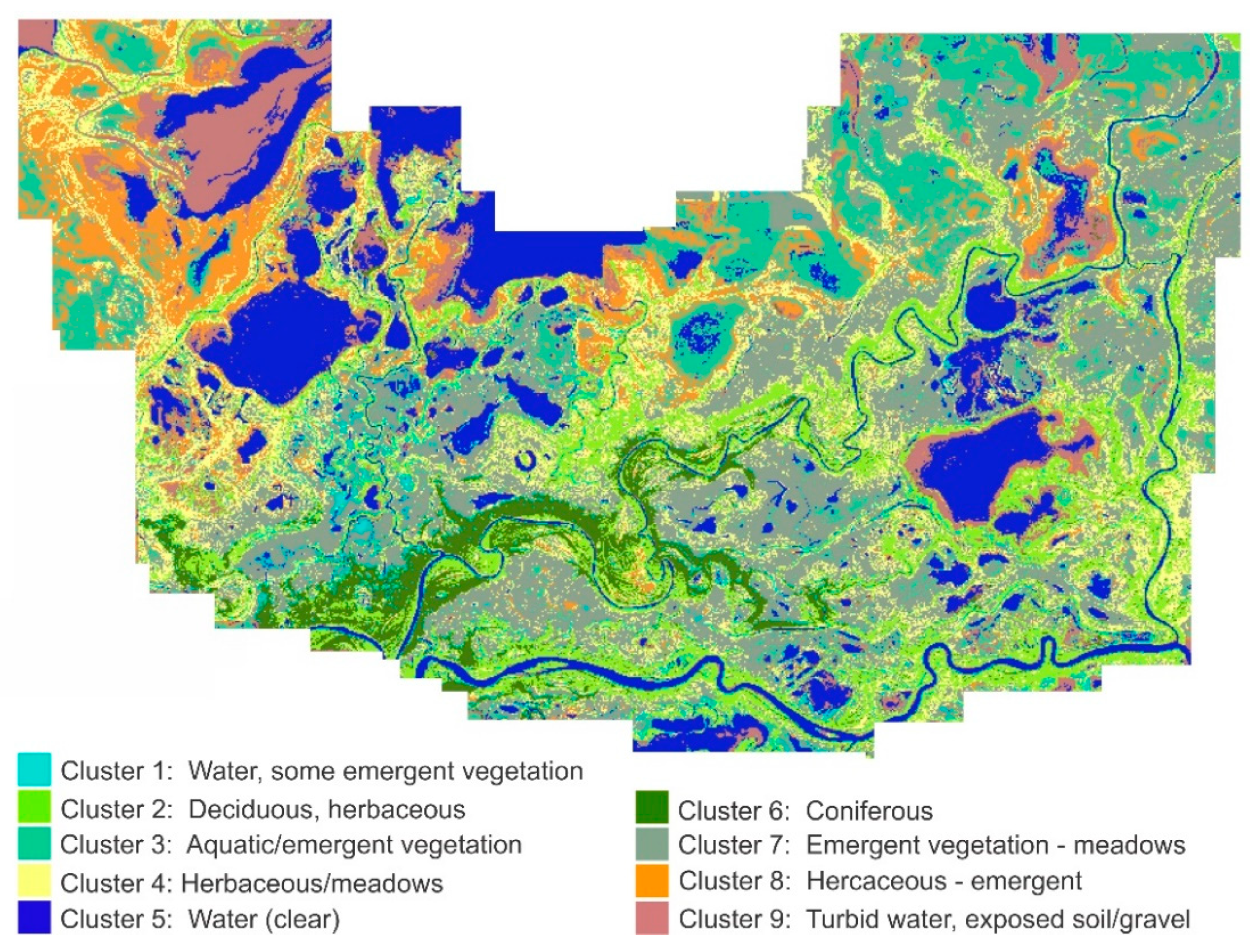
The study area was originally classified based on an integration of Sentinel-2 imagery and airborne LiDAR data into reflectance/structurally based cover classes. A detailed description of the process by which the cover classes were generated is provided in Peters et al. [18]. A visual, spatial summary of the segmentation of the landscape is provided in Figure 4, with the cluster numbering sequence retained in this study for the description of the behavior of the time series-based VI.
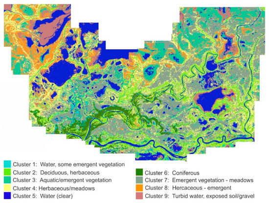
Figure 4.
A spatial representation of the structural classes of the cover for the study area. Reproduced with permission from Peters et al. [18].
3.2. Spectral Indices
As a precursor to our analysis of the consistency of the annual vegetative response, the degree and persistence of wetting conditions throughout the 2018 and 2019 growing seasons were examined. The MNDWI originally proposed by McFeetters [32] for LANDSAT MSS data, and later modified by Du et al. [33] to utilize the longer wavelengths on the ETM+ and Sentinel-2 sensors was selected to describe the land surface wetness. fAPAR and LAI were also chosen as they more closely describe meaningful vegetated conditions [15].
LAI is defined as half of the total foliage area per unit ground area [34], and has been used extensively as a proxy for physical and biological plant processes [35,36]. Sellers [37] noted that there was a maximum PAR absorption at LAI of 2 to 3, with absorption saturation >3 resulting in no change with changes in LAI. Sellers [37] also notes that there is some correspondence between area-based physiological processes and multi-spectrally based indices, but that the relationships are attenuated by effects of vegetation species, leaf orientation, LAI, and amount of plant litter. However, a low LAI was interpreted as an indicator of area physiological response to environmental inputs.
VIs used in this work were derived through the Sentinel Application Platform (SNAP) tool as published by the European Space Agency (ESA). The SNAP algorithm, used to derive the indices, was calibrated to rely on Level 1c or TOA reflectance data for the derivation of the indices. The algorithms behind each of the indices are described by Weiss and Baret [9].
3.3. Hydrometeorological Data
To evaluate the relative differences in hydrology and meteorology influencing the PAD for the two years of image sequences, flow on the lower Athabasca River at the Embarras Airport hydrometric station (07DD001) entering the AOI were obtained from the Water Survey of Canada [38] and the air temperature and precipitation data from the Meteorological Service of Canada for the nearby climate station at Fort Chipewyan (~30–40 km to the north of the AOI) available through the Government of Alberta portal [39]. A 1st of April snowpack index was calculated from accumulating the daily total precipitation from 1 November to 31 March [22]. The date of the spring 0 °C isotherm was calculated as the first positive air temperature along a 31-day running means [40]. Potential evapotranspiration was estimated using the Hamon [41] model based on daylength and air temperature that was validated for wetlands in the AOI by Peters et al. [27].
4. Results
4.1. Comparison of Wetting Conditions for the 2018 and 2019 Growing Seasons
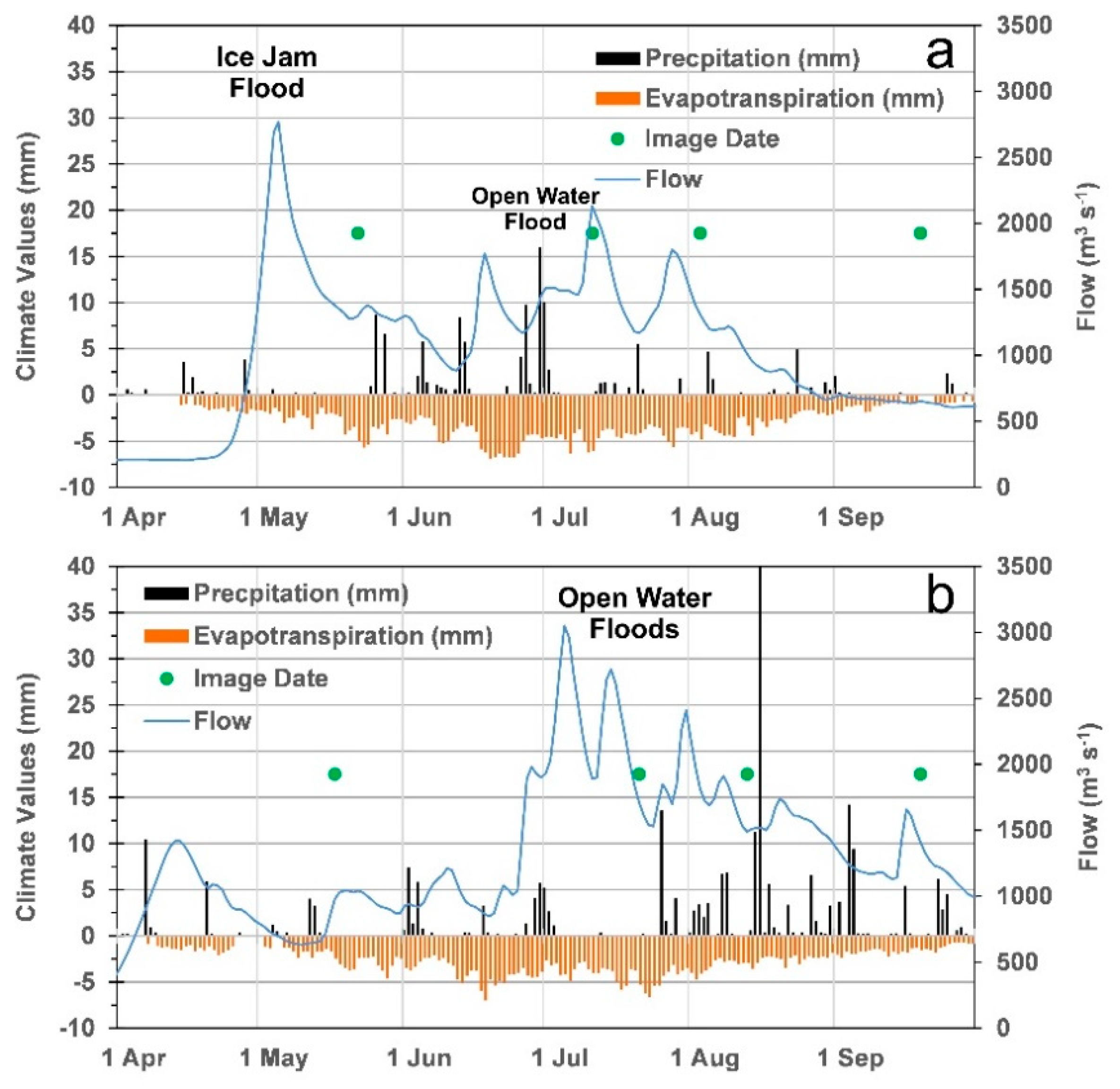
Compared to the 30-year mean climate, both study years 2018 and 2019 were slightly cooler than normal, received less than normal annual precipitation, and experienced above and below normal rates of total potential evapotranspiration, respectively (Table 2). Noteworthy to our analysis timeline was the spring ice-jam flood event of 2018 (later date of snowmelt as indicated by 0 °C isotherm, greater 1st of April snowpack index, and a larger spring peak flow magnitude coupled with mechanical ice breakup) around the lower Athabasca River, Embarras River and Mamawi Creek region that inundated adjacent lakes and wetlands in the delta floodplain covered by our AOI [42] (Figure 5). Furthermore, both summers experienced open-water flooding/connectivity events from high flows (i.e., >1750 m3 s−1) entering the Athabasca Delta as observed in several wetlands along the Mamawi Creek (unpublished data, Peters), with 2019 experiencing large and multiple summer overbanking events. Although the year 2019 had an earlier start to spring 0 °C isotherm, 2018 experienced considerably more potential evapotranspiration and less precipitation, leading to greater climatological net water loss during the growing season than in 2019 (i.e., precipitation minus potential evapotranspiration).
Table 2.
Hydrometeorological indices based on Fort Chipewyan (Alberta) data.
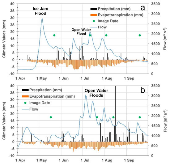
Figure 5.
Hydrometeorological data for the 2018 (a) and 2019 (b) study periods. Flow is on the lower Athabasca River at Embarras Airport just before entering the delta, potential evapotranspiration estimated via the Hamon (1961) model using climate data from Fort Chipewyan area.
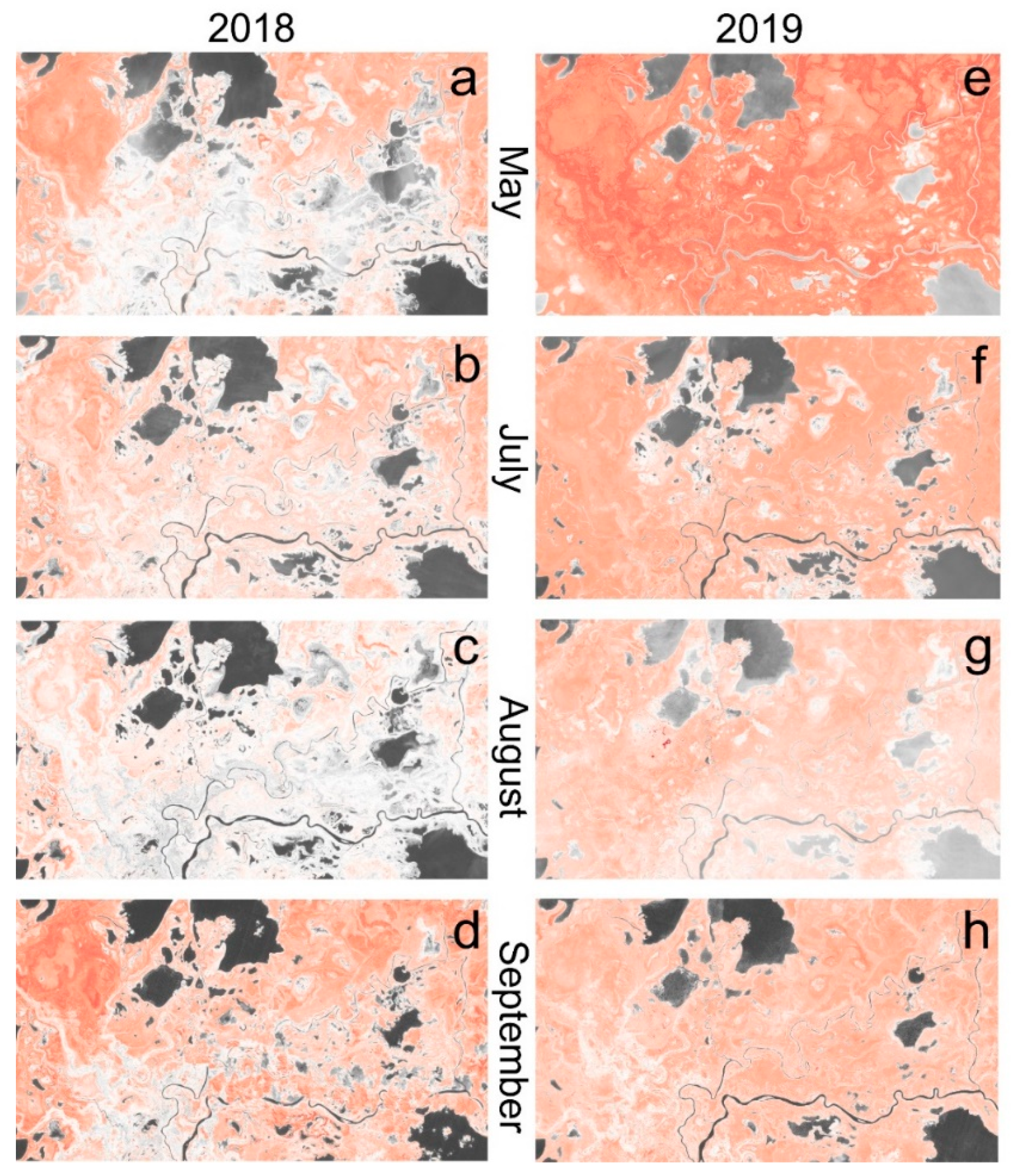
Figure 6 illustrates the spatial and temporal variations in the wetness conditions for the two years as determined by the MNDWI. As is evident in the two annual sequences of imagery, the 2018 data (Figure 6a–d) indicate that the May through August periods were characterized by wetter conditions than in the September scene. The levee and floodplain areas bordering the Athabasca River and Embarras River channels in the southern portion of the study area indicate extensive wetness. The intensity of this wetness decreases in July, increasing in the August and decreases in the September 2018 MNDWI image in the areas bordering the Athabasca River in the south. This is especially apparent in the early scenes, while the August scene indicates that there was a widespread increase in the MNDWI. If we relate the local temporal hydroclimatic patterns in Figure 5a to these MNDWI images, we can see that there were inundation events and several periods of rainfall prior to the acquisition dates for the three first scenes. There was a relatively dry period and declining flows leading up to the September acquisition, which is also reflected in the MNDWI output for that date.
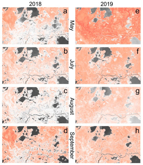
Figure 6.
Summary images of changes to the Modified Normalized Difference Water Index (MDNWI) over the two time periods used in this work: May, July, August and September images for 2018 (a–d) and 2019 (e–h), respectively. Grey indicates increasing wetness and red increasing dryness; all images stretched from −1 (drier—red) to 1 (wetter—grey).
The 2019 MNDWI imagery (Figure 6e–h) provides us with a different scenario, with an initially drier spring characterized with relatively lower spring flows (i.e., no ice-jam flooding), followed by a wetting period through August and then drying into the start of Autumn. These patterns are consistent with the hydrometeorological patterns presented in Figure 5b above. For the 2019 growing season, there was a period of precipitation which started prior to the July acquisition date, lasting throughout the summer until after the August imaging date. Moisture was also diverted into areas of the delta landscape as a result of several high flow events. There was an extended drying period prior to the September image.
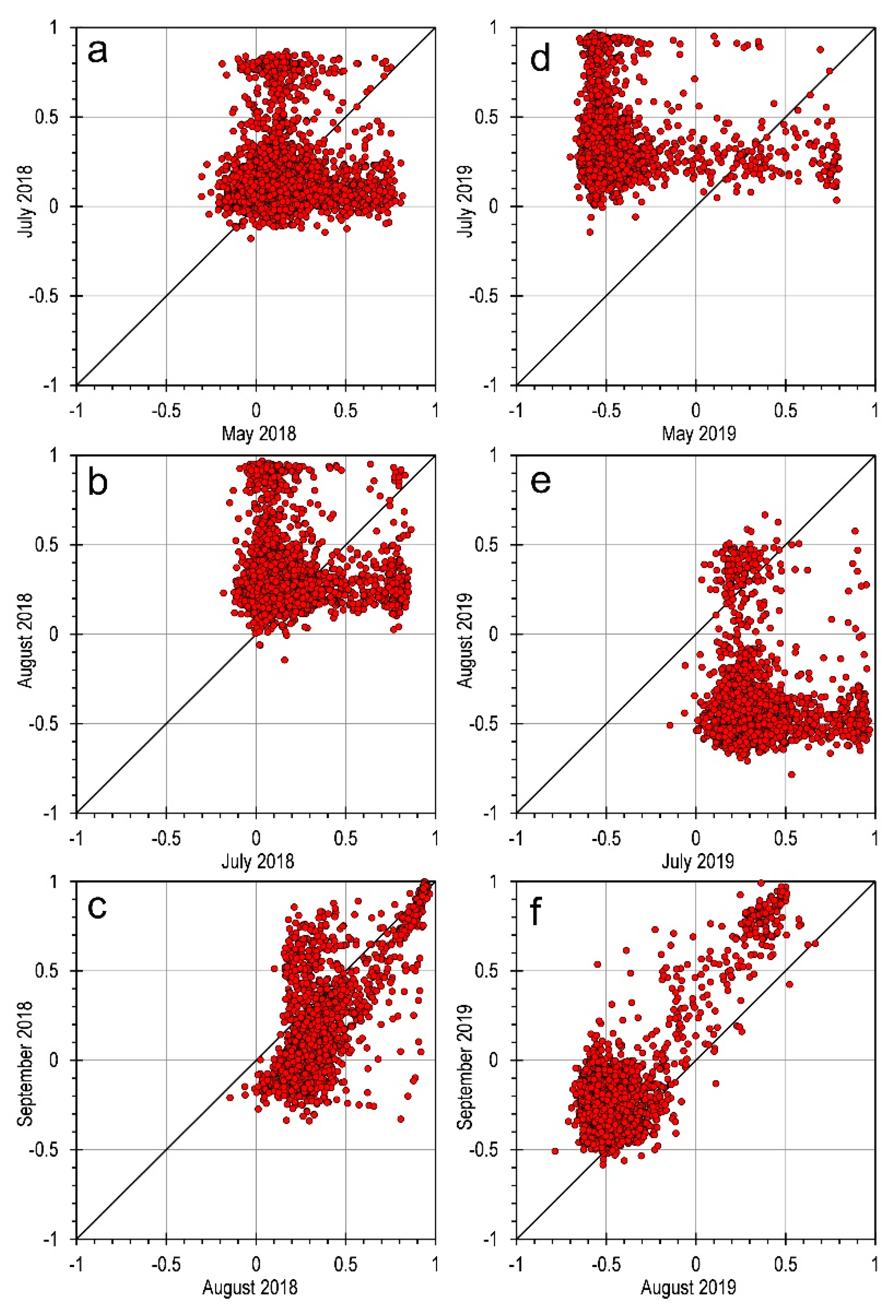
For a more detailed examination of the inter- and intra-year changes, we generated a set of 4000 randomly spaced points on which to base our sample. The distribution of these points is from south to north (see Figure 3 for polygons of points sampled), which corresponds to the observable variations in moisture content, especially as related to the 2018 flooding. These points were chosen because the areas bounded by the polygons: (i) encompassed the range of cover classes present in the study area; (ii) minimized the occurrence of standing water in the form of shallow ponds and lakes; and (iii) known to have experienced a range of flood timing and flood types. These same points were subsequently used below to address the changing vegetation indices. The intra-year comparison of the wetting patterns provided in Figure 7 shows that for 2018, there were inconsistencies between the early images. In comparing the July–August data, there was a general wetting of the area, while the August–September comparison was more organized, although the area was slightly wetter in the August scene. For 2019, the sample point comparison supports our more qualitative interpretation of Figure 6. Note that a 1:1 line was added to Figure 7 and Figure 8 to facilitate interpretation; in the case of no difference between the two periods, the points would lie on this line.
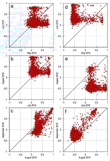
Figure 7.
Intra-year (2018 (a–c); 2019 (d–f)) comparison of the Modified Normalized Difference Water Index (MDNWI) for 2018–2019.
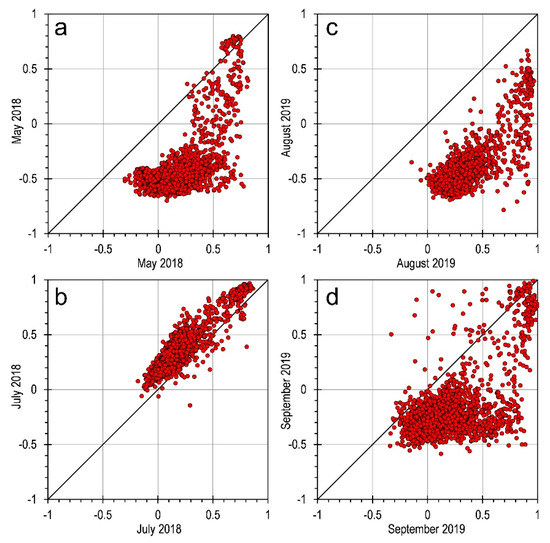
Figure 8.
Inter-year comparison of the Modified Normalized Difference Water Index (MDNWI) for 2018 vs. 2019 for May (a), July (b), August (c) and September (d).
The inter-year comparison presented in Figure 8 again supports our previous interpretation of Figure 6, with 2018 being considerably wetter in May, August and September than for the same periods in 2019 as indicated by MNDWI. Of the months examined, July appeared to be the more consistent between the two study years, but that could be attributed to the hydrometeorology of these specific years and may not extend to other years. Overall, wetness in the AOI of the Athabasca Delta was highly dynamic in response to various water inputs and outputs.
While meteorological—wetness associations would account for a general wetting or drying of the study area, they do not account for the spatial wetting/drying patterns. If we examine the May 2018 MNDWI image (Figure 6a–d), we see that the wetness was concentrated around the Athabasca and Embarras Rivers in the southern portions of the AOI, which is an important inflow zone of runoff generated from >150,000 km2, while the farther inland and lower elevation areas in the more northern deltaic portions of the study area remained dry relative to the higher areas closer to these rivers. This pattern is not as apparent in the time sequence of images for 2019 (Figure 6e–h). This is consistent with the 2018 flooding event, which was a result of ice jams temporarily impeding incoming spring freshet flow and generating extremely high waters that flowed over banks during that event. The year 2019, which provides us with a very different spatial wetting and drying pattern is more consistent with what we would expect with no spring ice jam, and summer rainfall-related processes enhanced by localized high flows overbanking channels into adjacent deltaic landscape, followed by drainage and drawdown.
In addition to the general wetting and drying pattern within the terrestrial portion of the delta, there were changes to the number and surface water extent of wetlands and small lakes scattered throughout the AOI. In examining Figure 6, we can see that in 2018, the small lakes and open water wetlands in the top half of the study area were larger and more numerous. The 2019 pattern is different in that the water bodies were less numerous in the early (May) image in comparison to July, which is particularly evident in the areas between the Athabasca and Embarras Rivers. MNDWI values surrounding these water bodies are lower than seen in the later data, indicating that not only has there been draining subsequent to inundations, but also a general drying of the landscape throughout the course of the growing season via evapotranspiration.
4.2. Response Comparison of Vegetation-Related Spectral Indices for 2018 and 2019
Capitalizing on the spatiotemporally changing hydrometeorological conditions in the study area, and the interdependency of the vegetation and the hydroperiod and moisture within wetland/lake basins and surrounding landscape, we examined the response of the vegetation indices during the 2018 and 2019 snow/ice-free seasons. To make this assessment, the same random point set described above was used to address the indices (LAI, fAPAR, MNDWI) from both years corresponding to the cover class cluster number found in Figure 4.
We performed a test of the separability of the clusters using a Kruskal–Wallis test. The results of these statistical tests on an intra- and inter-year basis are presented in Appendix Table A1, Table A2, Table A3 and Table A4. For the sake of clarity, the individual clusters were grouped into their interpreted cover classes (see Figure 4), and the examination was restricted to the non-water classes. This was done due to the transient nature of the water bodies over time and that LAI and fAPAR for water bodies may not be the most appropriate metrics to use. Kruskal–Wallis tests applied to the pooled samples indicated that there are no statistical differences between the datasets for the same periods for the two years (Table A2). The exception being for the fAPAR between May and July 2018, with the remaining two periods for 2018 showing no significant differences (p > 0.05). Consistent with observed fAPAR values in 2019, the three comparison periods for LAI returned no significant differences in the observed output. Table A4 summarizes the examination of the changes in the within-year cluster position and in all cases, the LAI and fAPAR index clusters differed seasonally.
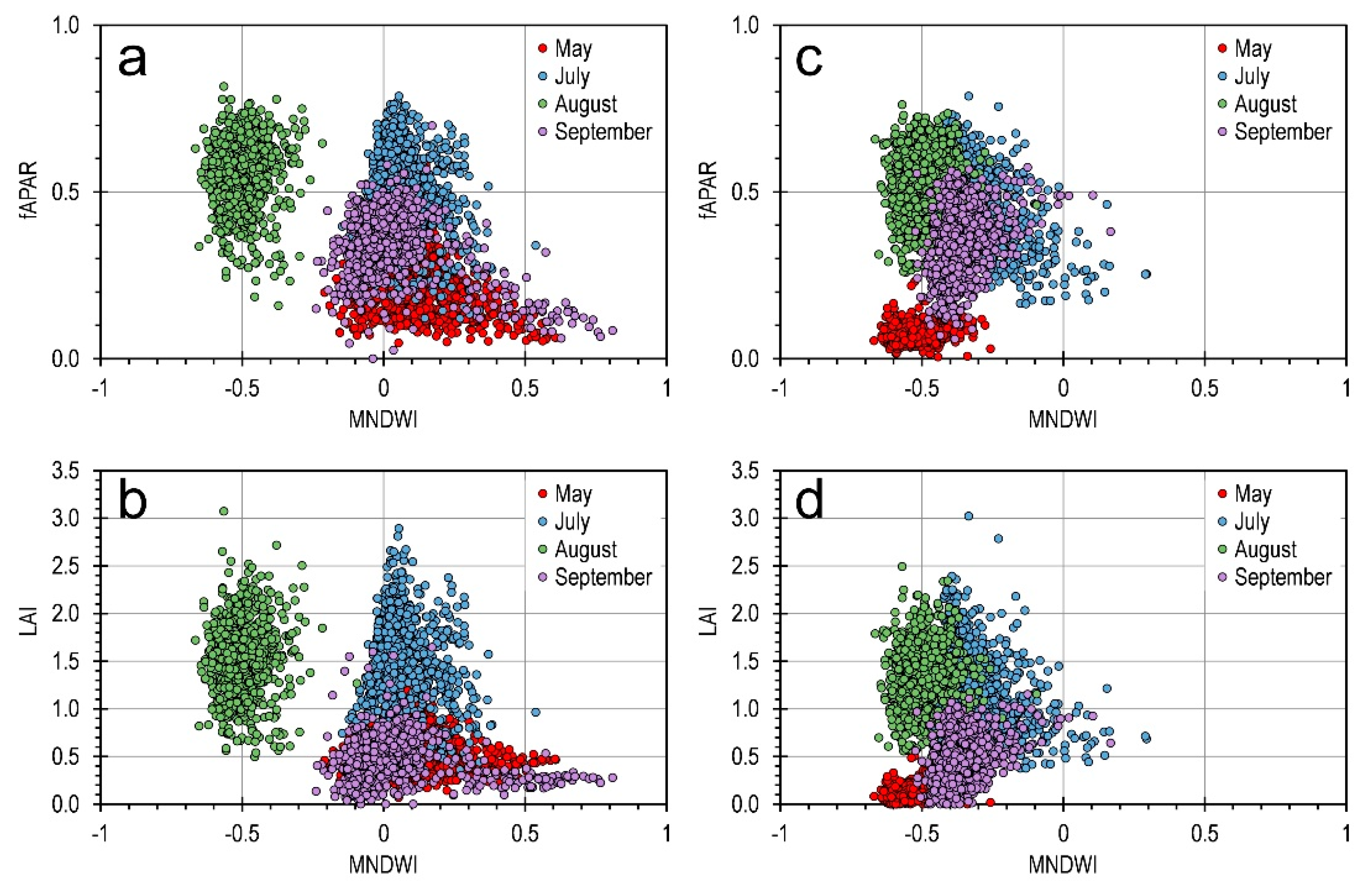
A summary of the LAI and fAPAR for both the 2018 and 2019 datasets are presented in Figure 9, Figure 10, Figure 11 and Figure 12. The behavior of the fAPAR and LAI during 2018 for the coniferous class is relatively consistent between periods (Figure 9). The early (May) fAPAR data cluster is slightly lower than that seen for the end of growing seasons (September) data. The July and August fAPAR clusters are at the same levels, even though the MNDWI levels for August are lower (drier). A similar pattern is observed with the 2018 LAI data with MNDWI. For the May 2019 fAPAR cluster, the levels are lower than we see for the other months. The fAPAR data for the three remaining 2019 acquisition dates are relatively consistent, although the MNDWI data ranges are not. The LAI data suggest that there was an increase in the overall LAI data from May through the summer acquisitions. However, the September cluster LAI levels decreased and are somewhat consistent with those seen in the May imagery. The differences between the May and September are primarily in the MNDWI levels. When we examine the relationships between fAPAR and LAI, we see a consistency between the May, July and August dates, with higher fAPAR values relative to LAI in September. These patterns can also be seen in the 2019 datasets, although there is less overlap between the May and July/August data.
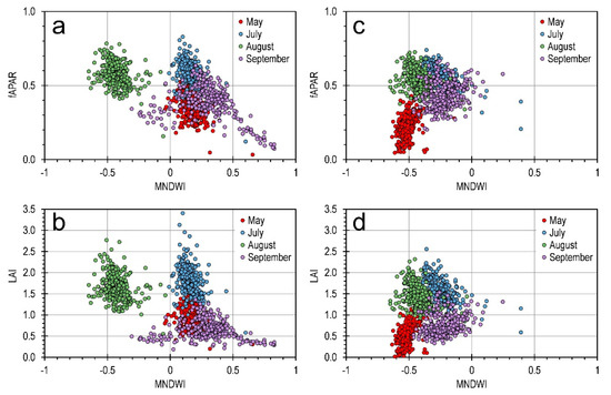
Figure 9.
Comparison of Coniferous class leaf area index (LAI) and absorbed photosynthetically available radiation (fAPAR) vs. Modified Normalized Difference Water Index (MDNWI) indices for the 2018 (a,b) and 2019 (c,d) growing seasons.
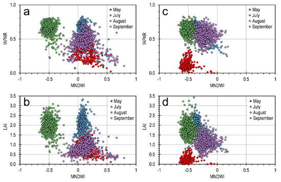
Figure 10.
Comparison of Deciduous class LAI and fAPAR vs. MDNWI indices for the 2018 (a,b) and 2019 (c,d) growing seasons. See Figure 9 for definition of acronyms.
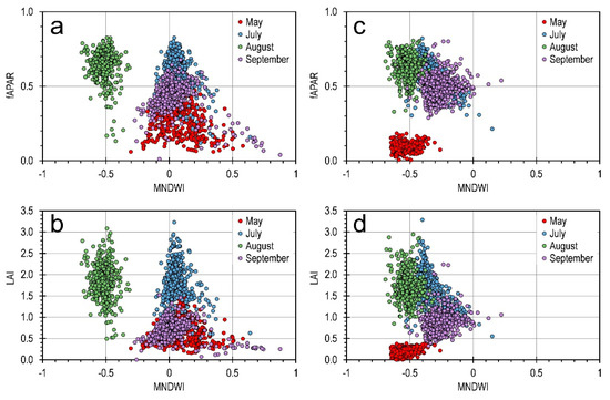
Figure 11.
Comparison of Herbaceous/Meadow class LAI and fAPAR vs. MDNWI indices for the 2018 (a,b) and 2019 (c,d) growing seasons. See Figure 9 for definition of acronyms.
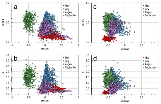
Figure 12.
Comparison of Emergent class LAI and fAPAR vs. MDNWI indices for the 2018 (a,b) and 2019 (c,d) growing seasons. See Figure 9 for definition of acronyms.
The Deciduous and Herbaceous/Meadow class patterns (Figure 10 and Figure 11) are similar to the those observed for the Coniferous class for the 2018 fAPAR data. There is a gradual increase in fAPAR from May through July and August, with a decrease into September. A similar pattern can be seen for the LAI values. In 2019, the fAPAR metrics were lower in the May image than we see for 2018, rising to equivalent levels in July and August but also maintaining a similar level into September. LAI patterns were similar again, with the May imagery being lower than the other three periods.
The Emergent vegetation (Figure 12) behaved differently than for the other three classes observed in that the 2018 early (May) fAPAR data are consistent with the observations for July and September, and that there is little change in this index for these three observation dates. The LAI data indicate less overlap between the early/late and mid-season values. For the 2019 fAPAR data, the pattern observed is more consistent with the other cover classes; however, the clustering is not as tight in this class as in the other three.
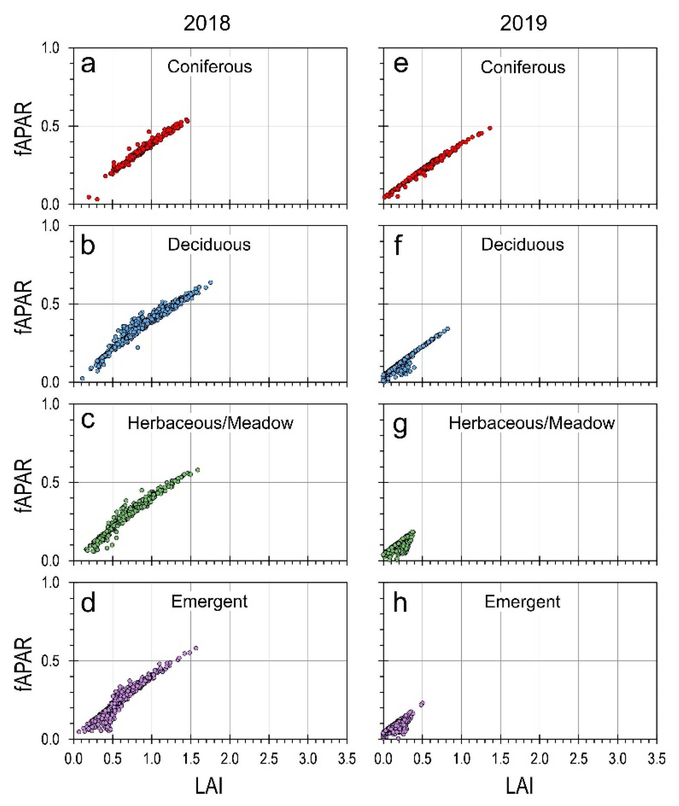
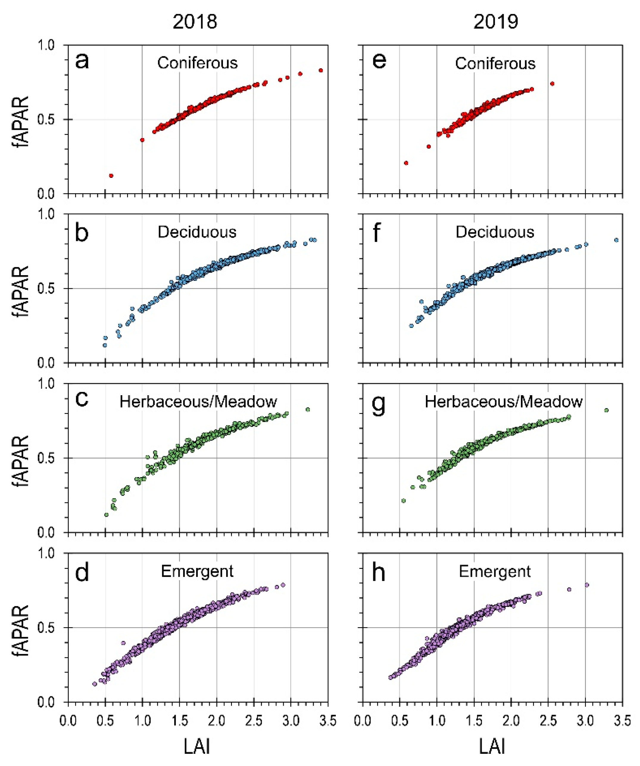
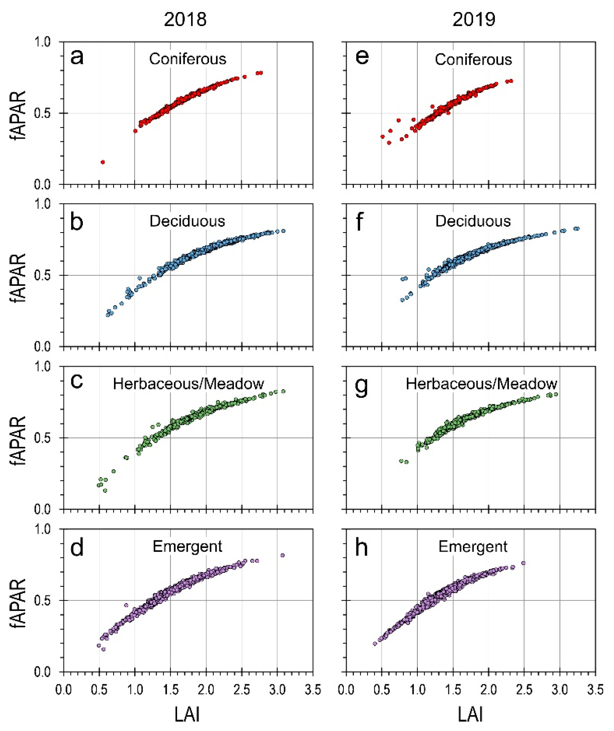
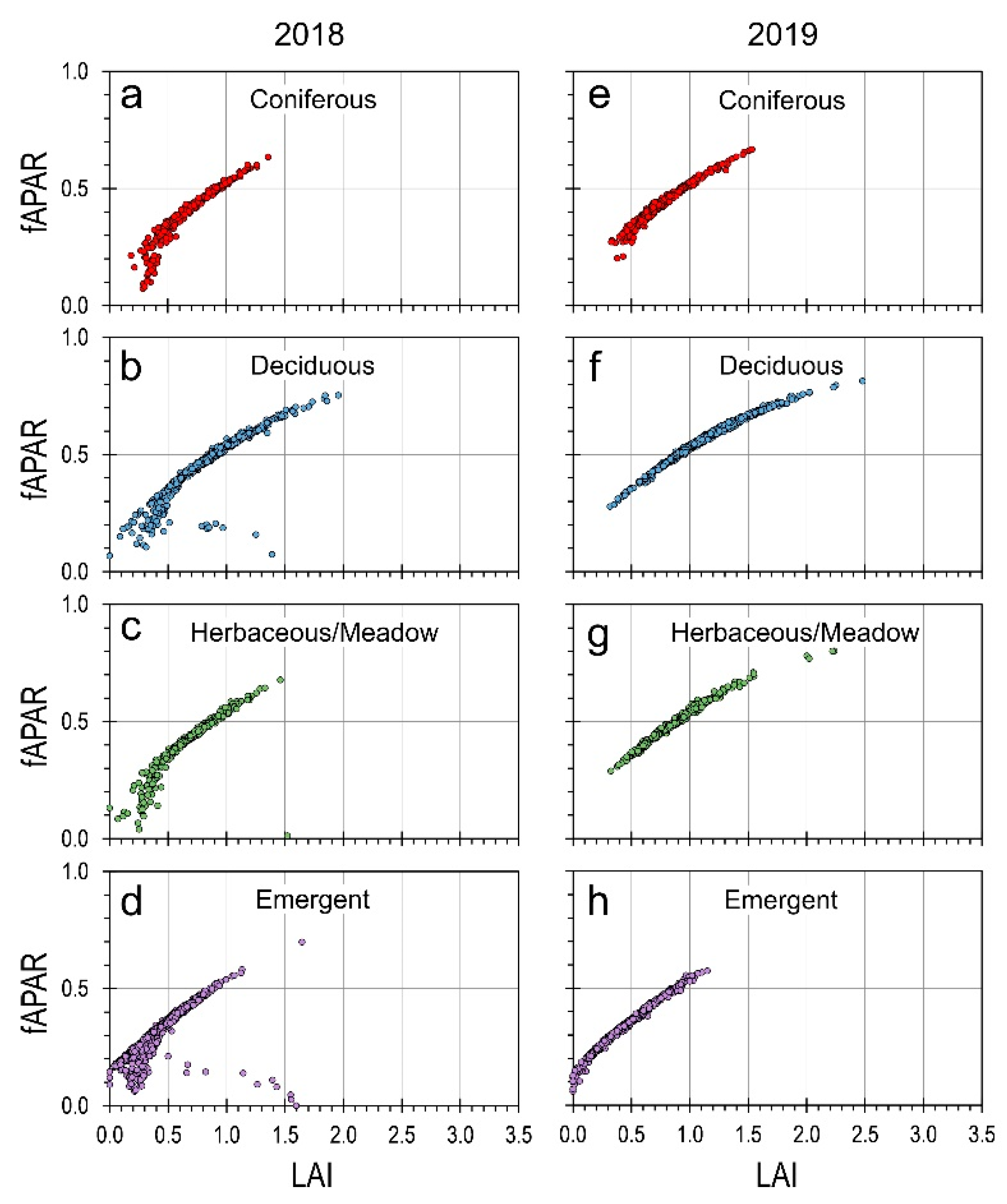
Figure 13, Figure 14, Figure 15 and Figure 16 summarize the relationship of fAPAR vs. LAI for the four vegetation classes (Coniferous, Deciduous, Herbaceous/Meadow, Emergent) for the sequences of images over the growing season of both study years. The May comparisons indicate a slightly broader range in LAI in the 2019 Coniferous samples than in 2018. The 2018 data also display a slight increase in the fAPAR for this image date. The Deciduous, Herbaceous/Meadow, and Emergent classes all show a much greater range in the 2018 indices than found in 2019. All three classes suggest a much lower level of development/green-up than is the case for the Coniferous class in 2019. The July and August data both yield similar patterns for both dates. The September data indicate slightly higher fAPAR levels in 2018, but also less organized fAPAR levels at lower LAI. This may suggest the initial onset of senescence for this later near Fall date, when mean daily air temperatures dropped below 5 °C and daylength shortened to <12 h.
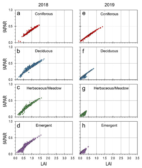
Figure 13.
May comparison of absorbed photosynthetically available radiation (fAPAR) vs. emergent leaf area index (LAI) for the 2018 (a–d) and 2019 (e–h) for the Coniferous, Deciduous, Herbaceous/Meadow and Emergent classes.
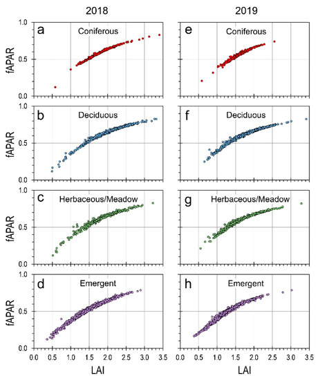
Figure 14.
July comparison of absorbed fAPAR vs. LAI for the 2018 (a–d) and 2019 (e–h) for the Coniferous, Deciduous, Herbaceous/Meadow and Emergent classes. See Figure 13 for definition of acronyms.
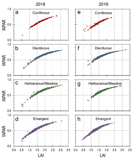
Figure 15.
August comparison of fAPAR vs. LAI for the 2018 (a–d) and 2019 (e–h) for the Coniferous, Deciduous, Herbaceous/Meadow and Emergent classes. See Figure 13 for definition of acronyms.
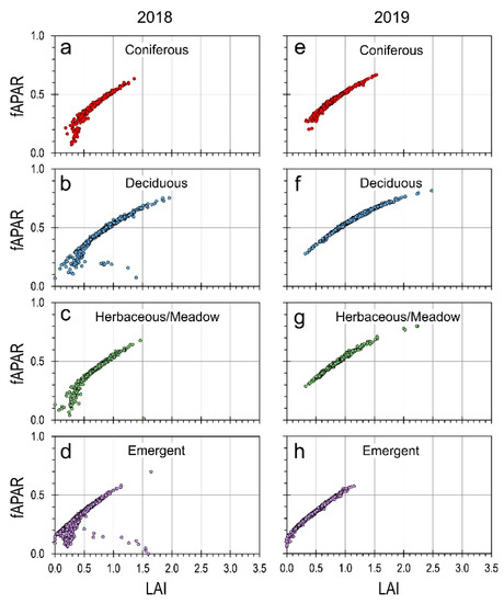
Figure 16.
September comparison of fAPAR vs. LAI for the 2018 (a–d) and 2019 (e–h) for the Coniferous, Deciduous, Herbaceous/Meadow and Emergent classes. See Figure 13 for definition of acronyms.
5. Discussion
The wetting patterns observed through the MNDWI spatiotemporal sequences presented in Figure 6 indicate that water dispersal in a complex, cold-regions wetland-lake landscape can be tracked through the use of EO data such as those acquired by the Sentinel-2 platform. The observed patterns in the 2018 dataset clearly indicate that the spring wetting radiated out from the major river and distributary channels that feed into the Athabasca Delta sector of the PAD. It is interesting to note that the areas to the north of our study area, which are generally at lower elevations and in closer proximity to the large central lakes (Lake Athabasca, Mamawi Lake, Lake Claire), were distant from and subsequently not as affected by ice-jam flooding, and thus, seen as drier than the southern areas more proximal to the river channels. It is also notable in the 2018 July and August data that the image acquisitions follow periods of rainfall and high flow events which would account for the increasing wetness, and that there was a drying pattern in the September image date consistent with the period of little rainfall immediately preceding the acquisition.
The wetting signal for 2019 was very different given that there was a relatively small spring runoff and no ice jams to divert water onto the landscape early in the growing season. The May image reveals a relatively dry study area that was influenced mostly by a local, below normal snowmelt amount. Wetting occurred throughout July and August consistent with a wetter mid-summer from higher rainfall and high flow-driven inundations of areas proximal to the river channels (e.g., Mamawi Creek). However, these areas were not as spatially pronounced as those affected by an ice-induced flood mechanism, which was capable of shunting water farther inland and into more elevated floodplain areas [19]. Similar to 2018, a general drying period prior to the September image date was seen in 2019.
The observed patterns in Figure 9, Figure 10, Figure 11 and Figure 12 are generally consistent with those observed by Kozlov et al. [43] who note that for large boreal wetlands in Russia, there is a general increase in fAPAR during the year peaking at around June. The wetter “marsh” vegetation, they note, has fAPAR peaks in the order of 0.8, while the woodland values peak at fAPAR 0.5–0.6. In our study, we see somewhat higher fAPAR levels with the coniferous samples for 2018, but a lower peak in 2019. Deciduous stands are consistent between the two years. Herbaceous samples peak at 0.8 in both 2018 and 2019, which is in line with the observations reported by Kozlov et al. [43]. What is particularly interesting to observe in Figure 9, Figure 10, Figure 11 and Figure 12 is the consistent cyclical nature of the point distributions patterns. The exception is in the case of the early season (May) observations, which appear to be more consistent with variations in the hydroclimate and flooding data. The patterns of observations from the later parts of the growing season may speak more to the influence of the long periods of solar insolation experienced in northern regions, which may dominate the growth cycle rather than water being the main growth-influencing variable (see expansion of this point below).
The relationship between fAPAR and LAI as described in Figure 13, Figure 14, Figure 15 and Figure 16 for the woodland samples (coniferous and deciduous) is typically linear for lower LAI values, but when considering the entire range of LAI, values tend towards a nonlinear relationship towards the upper end of the LAI range (LAI > 2.0). This can be interpreted as a decreasing sensitivity of satellite-derived LAI to describe changes in fAPAR values during the mid-summer period when the foliage is at its peak. This is consistent with observations from others that have examined the behavior of vegetation indices as they relate to vegetation structure [44,45]. An interesting observation from the data point in Figure 13, Figure 14, Figure 15 and Figure 16 is that the relationship between LAI and fAPAR is highly correlated. These two indices were chosen as they were thought to represent the canopy reaction to environmental inputs at different time scales (fAPAR more immediate, LAI more delayed). The take-away from this observation is that the LAI-based index could be used as a surrogate for fAPAR and foliar functioning. This is an important detail if we transition to a LANDSAT-based archive, which contains a longer time series, but with fewer spectral bands on which to derive a more limited set of vegetation indices.
As discussed above, the daily hydrometeorological data summarized in Figure 5 provide some insight as to the key environmental variables and their potential impact on the observed EO data. The MNDWI data for May 2018 map a general wetter surface, the cause of which may be related to the snowmelt/rainfall immediately preceding the May acquisition. However, this does not explain the spatial distribution of the MNDWI values observed in Figure 6. The wetness patterns for 2018, especially in the early image, radiate out from the larger river channels from south to north, which is more reflective of the spring flooding episode, rather than weather-related factors. While the MNDWI values for the 2019 map are spatially more homogeneous and indicate a drier overall surface over the growing season, there does not seem to be as dramatic a correlation with the wetter rainfall and peak flow period recorded in the weeks prior to the August image date. The sampled fAPAR and LAI values for those two image dates also indicate a consistency between the mid-summer sample dates for the two years. It is predominantly the May samples that provide a major difference between the two study years. The 2018 data suggest a higher level of photosynthetic activity and leaf area in the May data than observed for the same month in 2019. This is in spite of the fact that the spring melt commenced earlier in 2019 than it did in 2018. However, the May mean air temperature in 2018 was 4 °C higher than in 2019 (10.8 °C vs. 6.2 °C, respectively), promoting greater vegetation growth. The July and August observations suggest that the LAI and fAPAR measurements normalize during the mid-summer period and that the supposed effects of the spring flooding are mitigated, unless the occurrence of subsequent inundation events.
6. Conclusions
While this work examined one extensive spring ice-jam flooding and one less extensive open-water flooding year, there was an apparent early biological response to the former. These results demonstrate the utility of using indices such as MNDWI, fAPAR and LAI to track vegetation responses in a complex, cold-regions deltaic wetland ecosystem to two separate and differing seasonal wetting cycles. Future work utilizing a longer record, incorporating various combinations of large vs. small snowmelt years, as well as both flooding and non-flooding years, should provide a greater insight into the biological processes across the PAD. As the Sentinel-2 data archive grows, there will be an opportunity to expand this work to include multiple wetting and drying cycles, as well as examine lag times inherent in the response to various hydroclimatic conditions. Integrating the EO-based methodology outlined in this paper into an environmental monitoring framework to support ecosystem assessments, such as for the Wood Buffalo National Park World Heritage Action Plan [46] and Canada-Alberta Oil Sands Monitoring Program [47], will provide an opportunity to assess potential cumulative effects from regional climate change/variability, flow regulation and mining on the downstream PAD region ecosystem.
Author Contributions
Conceptualization, D.L.P., K.O.N. and R.S.; methodology, K.O.N., D.L.P. and R.S.; software, K.O.N., D.L.P. and R.S.; validation, K.O.N., D.L.P. and R.S.; formal analysis, K.O.N., D.L.P. and R.S.; investigation, D.L.P., K.O.N. and R.S.; resources, D.L.P., K.O.N. and R.S.; Data curation, D.L.P., K.O.N. and R.S.; writing—original draft preparation, D.L.P., K.O.N. and R.S.; writing—review and editing, D.L.P., K.O.N. and R.S.; visualization, D.L.P., K.O.N. and R.S.; supervision, D.L.P. and K.O.N.; project administration, D.L.P. and K.O.N.; funding acquisition, D.L.P. and K.O.N. All authors have read and agreed to the published version of the manuscript.
Funding
This work was funded by Environment and Climate Change Canada (ECCC) and the Oil Sands Monitoring (OSM) Program. This work is contribution to the OSM Program but does not necessarily reflect the position of the Program.
Acknowledgments
This work was initiated and supported by Environment and Climate Change Canada (ECCC) through several programs and projects: Oil Sands Monitoring (OSM) Program “Acquisition of Aerial High Resolution Digital Ground Terrain Information in the Peace-Athabasca Delta” and “Design of a Deltaic Wetland Ecosystem Health Monitoring” Projects; Climate Change and Adaptation (CCA) Program; ECCC Grants and Contributions to the University of Victoria; LookNorth Funding to Terra Remote Sensing Inc that conducted the aerial surveys. This work was partially funded under the OSM Program and is a contribution to the Program but does not necessarily reflect the position of the program.
Conflicts of Interest
The authors declare no conflict of interest.
Appendix A
Table A1.
Kruskal–Wallis test results for between year separability comparison of leaf area index (LAI) and absorbed photosynthetically available radiation (fAPAR). The presence of *** denotes that the null hypothesis was rejected and that the samples are significantly different at p = 0.05 level.
Table A1.
Kruskal–Wallis test results for between year separability comparison of leaf area index (LAI) and absorbed photosynthetically available radiation (fAPAR). The presence of *** denotes that the null hypothesis was rejected and that the samples are significantly different at p = 0.05 level.
| fAPAR | May 2018 | July 2018 | August 2018 | September 2018 |
| May 2019 | - | |||
| July 2019 | - | |||
| August 2019 | - | |||
| September 2019 | - | |||
| LAI | May 2018 | July 2018 | August 2018 | September 2018 |
| May 2019 | - | |||
| July 2019 | - | |||
| August 2019 | - | |||
| September 2019 | - |
Table A2.
Kruskal–Wallis test results for fAPAR between adjacent image acquisitions dates. The presence of *** denotes that the null hypothesis was rejected and that the samples are significantly different at p = 0.05 level.
Table A2.
Kruskal–Wallis test results for fAPAR between adjacent image acquisitions dates. The presence of *** denotes that the null hypothesis was rejected and that the samples are significantly different at p = 0.05 level.
| fAPAR | July 2018 | August 2018 | September 2018 |
| May 2018 | *** | ||
| July 2018 | - | ||
| August 2018 | - | ||
| fAPAR | July 2019 | August 2019 | September 2019 |
| May 2019 | - | ||
| July 2019 | - | ||
| August 2019 | - |
Table A3.
Kruskal–Wallis test results for LAI between adjacent image acquisitions dates. The presence of *** denotes that the null hypothesis was rejected and that the samples are significantly different at p = 0.05 level.
Table A3.
Kruskal–Wallis test results for LAI between adjacent image acquisitions dates. The presence of *** denotes that the null hypothesis was rejected and that the samples are significantly different at p = 0.05 level.
| LAI | July 2018 | August 2018 | September 2018 |
| May 2018 | - | ||
| July 2018 | - | ||
| August 2018 | - | ||
| LAI | July 2019 | August 2019 | September 2019 |
| May 2019 | - | ||
| July 2019 | - | ||
| August 2019 | - |
Table A4.
Kruskal–Wallis test results for comparison of separation metrics (LAI and fAPAR) based on vegetation cover class/clusters through time for LAI between adjacent image acquisitions dates. The presence of *** denotes that the null hypothesis was rejected and that the samples are significantly different at p = 0.05 level.
| Conifer 2018 (Cluster 6) | May–July | July–August | August–September |
| fAPAR | *** | *** | *** |
| LAI | *** | *** | *** |
| Conifer 2019 (Cluster 6) | May–July | July–August | August–September |
| fAPAR | *** | *** | *** |
| LAI | *** | *** | *** |
| Deciduous 2018 (Cluster 2) | May–July | July–August | August–September |
| fAPAR | *** | *** | *** |
| LAI | *** | - | *** |
| Deciduous 2019 (Cluster 2) | May–July | July–August | August–September |
| fAPAR | *** | *** | *** |
| LAI | *** | *** | *** |
| Herbaceous/Meadows 2018 (Cluster 4 and 8) | May–July | July–August | August–September |
| fAPAR | *** | *** | *** |
| LAI | *** | - | *** |
| Herbaceous/Meadows 2019 (Cluster 4 and 8) | May–July | July–August | August–September |
| fAPAR | *** | *** | *** |
| LAI | *** | *** | *** |
| Emergent 2018 (Cluster 3 and 7) | May–July | July–August | August–September |
| fAPAR | *** | *** | *** |
| LAI | *** | - | *** |
| Emergent 2019 (Cluster 3 and 7) | May–July | July–August | August–September |
| fAPAR | *** | *** | *** |
| LAI | *** | *** | *** |
References
- U.S. Environmental Protection Agency (EPA). Why Are Wetlands Important? Available online: https://www.epa.gov/wetlands/why-are-wetlands-important (accessed on 29 August 2020).
- Ramsar Homepage. Available online: https://www.ramsar.org/ (accessed on 29 August 2020).
- Dennison, W.C.; Orth, R.J.; Moore, K.A.; Stevenson, J.C.; Carter, V.; Kollar, S.; Bergstrom, P.W.; Batiuk, R.A. Assessing water quality with submersed aquatic vegetation. BioScience 1993, 43, 86–94. [Google Scholar] [CrossRef]
- Adam, E.; Mutanga, O.; Rugege, D. Multispectral and hyperspectral remote sensing for identification and mapping of wetland vegetation: A review. Wetl. Ecol. Manag. 2010, 18, 281–296. [Google Scholar] [CrossRef]
- Bannari, A.; Morin, D.; Bonn, F.; Huete, A.R. A review of vegetation indices. Remote Sens. Rev. 1995, 13, 95–120. [Google Scholar] [CrossRef]
- Xue, J.; Su, B. Significant remote sensing vegetation indices: A review of developments and applications. J. Sens. 2017, 2017, e1353691. [Google Scholar] [CrossRef] [Green Version]
- Mutanga, O.; Skidmore, A.K. Narrow band vegetation indices overcome the saturation problem in biomass estimation. Int. J. Remote. Sens. 2004, 25, 3999–4014. [Google Scholar] [CrossRef]
- ESA Sentinel-2 European Space Agency. Available online: http://www.esa.int/Applications/Observing_the_Earth/Copernicus/Sentinel-2 (accessed on 21 March 2021).
- Weiss, M.; Baret, F. Sentinel-2 ToolBox Level2 Products: LAI, FAPAR, FCOVER Version 1.1. 2016. Available online: http://step.esa.int/docs/extra/ATBD_S2ToolBox_L2B_V1.1.pdf (accessed on 10 August 2021).
- Kamenova, I.; Dimitrov, P. Evaluation of Sentinel-2 vegetation indices for prediction of LAI, FAPAR and FCover of winter wheat in Bulgaria. Eur. J. Remote Sens. 2021, 54, 89–108. [Google Scholar] [CrossRef]
- Gower, S.T.; Kucharik, C.J.; Norman, J.M. Direct and indirect estimation of leaf area index, fAPAR, and net primary production of terrestrial ecosystems. Remote Sens. Environ. 1999, 70, 29–51. [Google Scholar] [CrossRef]
- Gobron, N.; Pinty, B.; Taberner, M.; Merlin, F.; Widlowski, J.-L.; Verstraete, M.M. Monitoring FAPAR over land surfaces with remote sensing data. In Remote Sensing for Agriculture, Ecosystems, and Hydrology V; International Society for Optics and Photonics: Bellingham, WA, USA, 2004; Volume 5232, pp. 237–244. [Google Scholar]
- Ogutu, B.O.; Dash, J.; Dawson, T.P. Evaluation of the influence of two operational fraction of absorbed photosynthetically active radiation (FAPAR) Products on terrestrial ecosystem productivity modelling. Int. J. Remote Sens. 2014, 35, 321–340. [Google Scholar] [CrossRef]
- Liu, N.; Treitz, P. Modelling high arctic percent vegetation cover using field digital images and high resolution satellite data. Int. J. Appl. Earth Obs. Geoinf. 2016, 52, 445–456. [Google Scholar] [CrossRef]
- Baret, F.; Guyot, G. Potentials and limits of vegetation indices for LAI and APAR assessment. Remote Sens. Environ. 1991, 35, 161–173. [Google Scholar] [CrossRef]
- Bonan, B.B. Importance of leaf area index and forest type when estimating photosynthesis in boreal forests. Remote Sens. Environ. 1993, 43, 303–314. [Google Scholar] [CrossRef]
- Putzenlechner, B.; Castro, S.; Kiese, R.; Ludwig, R.; Marzahn, P.; Sharp, I.; Sanchez-Azofeifa, A. Validation of sentinel-2 FAPAR products using ground observations across three forest ecosystems. Remote Sens. Environ. 2019, 232, 111310. [Google Scholar] [CrossRef]
- Peters, D.L.; Niemann, K.O.; Skelly, R. Remote sensing of ecosystem structure: Fusing passive and active remotely sensed data to characterize a deltaic wetland landscape. Remote Sens. 2020, 12, 3819. [Google Scholar] [CrossRef]
- Peters, D.L.; Prowse, T.D.; Pietroniro, A.; Leconte, R. Flood hydrology of the peace-athabasca delta, Northern Canada. Hydrol. Process. 2006, 20, 4073–4096. [Google Scholar] [CrossRef]
- Peters, D.L.; Buttle, J.M. The effects of flow regulation and climatic variability on obstructed drainage and reverse flow contribution in a Northern river–lake–Delta complex, Mackenzie basin headwaters. River Res. Appl. 2010, 26, 1065–1089. [Google Scholar] [CrossRef]
- Peters, D.L.; Prowse, T.D. Regulation effects on the Lower Peace River, Canada. Hydrol. Process. 2001, 15, 3181–3194. [Google Scholar] [CrossRef]
- Peters, D.L.; Prowse, T.D. Generation of streamflow to seasonal high waters in a freshwater delta, northwestern Canada. Hydrol. Process. 2006, 20, 4173–4196. [Google Scholar] [CrossRef]
- Peters, D.L.; Atkinson, D.; Monk, W.A.; Tenenbaum, D.E.; Baird, D.J. A multi-scale hydroclimatic analysis of runoff generation in the Athabasca River, Western Canada. Hydrol. Process. 2013, 27, 1915–1934. [Google Scholar] [CrossRef]
- Alexander, A.C.; Chambers, P.A. Assessment of seven canadian rivers in relation to stages in oil sands industrial development, 1972–2010. Environ. Rev. 2016, 24, 484–494. [Google Scholar] [CrossRef] [Green Version]
- PAD-PG. Peace-Athabasca Delta Project Group Technical Report: A Report on Low Water Levels in Lake Athabasca and Their Effect on the Peace-Athabasca Delta; Governments of Canada, Alberta and Saskatchewan: Canada, 1973; p. 176.
- Jaques, D.R. Topographic Mapping and Drying Trends in the Peace-Athabasca Delta, Alberta Using LANDSAT MSS Imagery; Report Prepared by Ecostat Geobotanical Surveys Inc. for Wood Buffalo National Park, Parks Canada: Fort Smith, NT, Canada, 1989. [Google Scholar]
- Peters, D.L.; Prowse, T.D.; Marsh, P.; Lafleur, P.M.; Buttle, J.M. Persistence of water within perched basins of the Peace-Athabasca Delta, Northern Canada. Wetl. Ecol. Manag. 2006, 14, 221–243. [Google Scholar] [CrossRef]
- Peters, D.L. Multi-Scale Hydroclimatic Controls on the Duration of Water in Perched Wetlands of a Cold Regions Delta, Northwestern Canada; Environment Canada: Saskatoon, SK, Canada, 2013; p. 43. [Google Scholar]
- Timoney, K.P. The Peace-Athabasca Delta: Portrait of a Dynamic Ecosystem; The University of Alberta Press: Edmonton, AB, Canada, 2013; ISBN 978-0-88864-730-6. [Google Scholar]
- Timoney, K. Landscape cover change in the Peace-Athabasca Delta, 1927–2001. Wetlands 2006, 26, 765–778. [Google Scholar] [CrossRef]
- Bush, A.; Monk, W.A.; Compson, Z.G.; Peters, D.L.; Porter, T.M.; Shokralla, S.; Wright, M.T.G.; Hajibabaei, M.; Baird, D.J. DNA metabarcoding reveals metacommunity dynamics in a threatened boreal wetland wilderness. Proc. Natl. Acad. Sci. USA 2020, 117, 8539–8545. [Google Scholar] [CrossRef] [Green Version]
- McFeetters, S.K. The use of the normalized difference water index (NDWI) in the delineation of open water features. Int. J. Remote Sens. 1996, 17, 1425–1432. [Google Scholar] [CrossRef]
- Du, Y.; Zhang, Y.; Ling, F.; Wang, Q.; Li, W.; Li, X. Water bodies’ mapping from Sentinel-2 imagery with modified normalized difference water index at 10-m spatial resolution produced by sharpening the SWIR band. Remote Sens. 2016, 8, 354. [Google Scholar] [CrossRef] [Green Version]
- Chen, J.M.; Black, T.A. Measuring leaf area index on plant canopies with branch architecture. Agric. For. Meteorol. 1991, 57, 1–12. [Google Scholar] [CrossRef]
- Moulin, S.; Bondeau, A.; Delecolle, R. Combining Agricultural crop models and satellite observations: From field to regional scales. Int. J. Remote Sens. 1998, 19, 1021–1036. [Google Scholar] [CrossRef]
- Running, S.W.; Baldocchi, D.D.; Turner, D.P.; Gower, S.T.; Bakwin, P.S.; Hibbard, K.A. A global terrestrial monitoring network integrating tower fluxes, flask sampling, ecosystem modeling and EOS satellite data. Remote Sens. Environ. 1999, 70, 108–127. [Google Scholar] [CrossRef]
- Sellers, P.J. Canopy reflectance, photosynthesis and transpiration. Int. J. Remote Sens. 1985, 6, 1335–1372. [Google Scholar] [CrossRef]
- ECCC HYDAT Water Survey Data Products 2020. Available online: https://www.canada.ca/en/environment-climate-change/services/water-overview/quantity/monitoring/survey/data-products-services.html (accessed on 1 May 2021).
- GOA Government of Alberta—Interpolated Weather Data Since 1961 for Alberta Townships. Available online: https://agriculture.alberta.ca/acis/township-data-viewer.jsp (accessed on 1 May 2021).
- Bonsal, B.; Prowse, T. Trends and variability in spring and autumn 0 °C-isotherm dates over Canada. Clim. Chang. 2003, 57. [Google Scholar] [CrossRef]
- Hamon, W.R. Estimating potential evapotranspiration. J. Hydraul. 1961, 87, 107–120. [Google Scholar]
- Remmer, C.R.; Owca, T.; Neary, L.; Wiklund, J.A.; Kay, M.; Wolfe, B.B.; Hall, R.I. Delineating extent and magnitude of river flooding to lakes across a northern delta using water isotope tracers. Hydrol. Process. 2020, 34, 303–320. [Google Scholar] [CrossRef] [Green Version]
- Kozlov, A.; Kozlova, M.; Skorik, N. A simple harmonic model for FAPAR temporal dynamics in the wetlands of the Volga-Akhtuba Floodplain. Remote Sens. 2016, 8, 762. [Google Scholar] [CrossRef] [Green Version]
- Aklilu Tesfaye, A.; Gessesse Awoke, B. Evaluation of the saturation property of vegetation indices derived from Sentinel-2 in mixed crop-forest ecosystem. Spat. Inf. Res. 2021, 29, 109–121. [Google Scholar] [CrossRef]
- Chernetskiy, M.; Gómez-Dans, J.; Gobron, N.; Morgan, O.; Lewis, P.; Truckenbrodt, S.; Schmullius, C. Estimation of FAPAR over croplands using MISR data and the earth observation land data assimilation system (EO-LDAS). Remote Sens. 2017, 9, 656. [Google Scholar] [CrossRef] [Green Version]
- WBNP. Development of a Multi-Jurisdiction Action Plan to Protect the World Heritage Values of Wood Buffalo National Park. 2019. Available online: https://www.pc.gc.ca/en/pn-np/nt/woodbuffalo/info/action (accessed on 10 August 2021).
- JOSM. The Joint Canada | Alberta Implementation Plan. for Oil Sands Monitoring Annual Report; Government of Canada: Ottawa, ON, Canada, 2012; p. 32. Available online: http://www.publications.gc.ca/site/eng/9.697128/publication.html (accessed on 10 August 2021).


Publisher’s Note: MDPI stays neutral with regard to jurisdictional claims in published maps and institutional affiliations. |
© 2021 by the authors. Licensee MDPI, Basel, Switzerland. This article is an open access article distributed under the terms and conditions of the Creative Commons Attribution (CC BY) license (https://creativecommons.org/licenses/by/4.0/).