Quality Scoring of the Fengyun 4A Clear Sky Radiance Product

Abstract

The Clear Sky Radiance (CSR) product has been widely used instead of Level 1 (L1) geostationary imager data in data assimilation for numerical weather prediction due to its many advantages concerning superobservation methodology. In this study, CSR was produced in two water vapor channels (channels 9 and channel 10, with wavelengths at 5.8–6.7 μm and 6.9–7.3 μm) of the Advanced Geostationary Radiation Imager aboard Fengyun 4A. The root mean square error (RMSE) between CSR observations and backgrounds was used as a quality flag and was predicted by cloud cover, standard deviation (STD), surface type, and elevation of a CSR field of view (FOV). Then, a centesimal scoring system based on the predicted RMSE was set to a CSR FOV that indicates its percentile point in the quality distribution of the whole FOV. Validations of the scoring system demonstrated that the biases of the predicted RMSE were small for all FOVs and that the score was consistent with the predicted RMSE, especially for FOVs with high scores. We suggest using this score for quality control (QC) to replace the QC of cloud cover, STD, and elevation of CSR, and we propose 40 points as the QC threshold for the two channels, above which the predicted RMSE of a CSR is superior to the RMSE of averaged clear-sky L1 data.

1. Introduction

Weather analysis and numerical weather prediction (NWP) models have benefitted from image data and retrieved motion vectors by water vapor (WV) channels at 6.7 μm, which are usually aboard geostationary satellites [1,2]. To date, all-sky assimilation of satellite radiance remains a significant challenge [3], and clear-sky radiance still has an important role in most operational NWP models worldwide. Neutral-to-positive impacts on forecast skill have been found in both global and regional models when clear-sky WV radiance or brightness temperature (BT) is assimilated. For example, Szyndel et al. [4] assimilated the WV radiances of Spinning Enhanced Visible and InfraRed Imager (SEVIRI) aboard the Meteosat-8 into the NWP model of European Centre for Medium-Range Weather Forecasts (ECMWF) and found a positive impact on wind and height field forecasts, which may result from a better assignment of moisture in the vertical direction. Stengel et al. [5] demonstrated the benefit of a regional NWP model’s analysis and forecasts gained by the assimilation of SEVIRI infrared radiances. The main direct impacts on the analysis were tropospheric humidity and wind increment, and positive impacts were revealed for almost all upper tropospheric variables in forecast verifications. Rani et al. [6] assimilated the clear-sky BTs of WV channels of the INSAT-3D imager into the assimilation and forecast system of the National Centre for Medium Range Weather Forecasting (NCMRWF), demonstrating a positive impact on the humidity and upper tropospheric wind fields, whereas the impact on the temperature field, particularly over the tropics, was neutral. Moreover, studies have shown that assimilating WV radiances would improve the forecasting of convective processes [7], coastal quantitative precipitation [8,9], and the overall tracking and intensity of tropical storms [10].

The Clear Sky Radiance (CSR) product for geostationary satellites has been developed for data assimilation in the NWP model and introduced into operation in ECMWF [11,12] and Japan Meteorological Agency (JMA) [13,14]. In a predefined assembly of pixels for imager WV channels, CSR, by a so-called superobservation methodology, is the average of the radiance or BT over all clear pixels in an assembly [15,16]. An advantage of the superobservation is that it greatly reduces the data volume when upscaling the resolution of the observation. Moreover, as the resolution of geostationary satellite imagers generally exceeds that of global models, the representation errors will also be reduced to gain consistency in the resolutions between the NWP model and satellite observations [17] when CSR is assimilated in NWP compared with L1 data. In another way, observations are assumed to be independent of each other in assimilation, and satellite data with high resolution must be thinned to reduce correlations with neighboring observations before they can be used in assimilations [18]. Studies have been conducted on thinning methods, such as uniformly spaced sampling, superobservation, and many adaptive thinning algorithms [19,20]. The superobservation method has been widely used in assimilations due to its simple algorithm, high ratio of data utilization, and low uncorrelated random error [21]. However, extra errors would be introduced by superobservations when using the averaged radiance or BT of clear-sky pixels to represent the whole segment in clear-sky situations.

Quality control (QC) is a primary process used in data assimilation. Generally, four QC processes must be implemented for the assimilation of clear-sky radiances. First, the quality of satellite L1 data closely corresponds to the parameters of instruments during their observation, and QC methods are necessary for these observations based on the working characteristics, which include the status of the satellite and instrument environment, the observational geometry, and the correctness of instrument calibration [22]. Second, a cloud detection method is necessary to remove the radiances contaminated by clouds. Spatial variability, represented by standard deviation (STD), is often used in cloud screening algorithm [23,24]. Next, limitations are often set to satellite observations, such as latitude, altitude, and surface type, for satellite field of views (FOV) so that the received radiances do not contain emissions of complicated surfaces. Setting a threshold on the observation minus background (O-B) is the last primary QC in assimilation. Large O-B may result from complex scatter radiative transfer in clouds or scale mismatches between observations and simulations. Even correct data should sometimes be rejected if they reflect processes that cannot be resolved on the scale of the grid system used in the analysis [25]. For the CSR product, the representativeness of averaged clear-sky pixels in superobservation segment should be considered for a large number of FOVs that are partly contaminated, and the QC scheme should be designed accordingly.

Fengyun 4A, the first satellite of the second-generation geostationary meteorological satellite in China, was launched on December 11, 2016 and located at 104.7°E. Among the four payloads on Fengyun 4A, the Advanced Geostationary Radiation Imager (AGRI) has a comparable performance with the most cutting-edge geostationary imager [26]. Fourteen channels were set in the AGRI, and there were two WV channels, 5.8–6.7 μm (channel 9) and 6.9–7.3 μm (channel 10), to detect the layer water vapor content in the mid-atmosphere with a 4-km resolution at nadir [27]. The remote sensing products of AGRI are highly qualified and have been widely utilized in many fields of atmospheric science [28,29]. For data assimilation, the impact on bias correction has been analyzed for AGRI radiance [30,31]. In this paper, CSR products were developed for the two WV channels of AGRI, and a scoring system was designed to indicate the CSR quality. Then, a QC scheme was set based on the score. In Section 2, an introduction to the CSR product and its quality flags is presented. Validations of the clear-sky screening and scoring system are shown in Section 3. In Section 4, we discuss the application of the CSR score. Conclusions and some discussion are given in Section 5.

2. Methodology

2.1. Superobservation of FY4A CSR

Duan et al. [21] pointed out that the larger the superobservation segment is, the smaller the uncorrelated random error of observation will be. However, fewer synoptic features would be presented in an observation with lower resolution. In this paper, we designed a superobservation strategy based on a resolution of 15 km for the operational Global and Regional Assimilation in Numerical Model and Prediction System (GRAPES) [32] of the China Meteorological Administration. Therefore, 3 × 3-pixel image segmentation is applied to AGRI L1 raw data, making the resolution 12 km at nadir, and all 3 × 3 pixels are referred to as the CSR FOV. Then, the geolocation, zenith angle, as well as azimuth angle to the sensor and sun for a CSR FOV were set to the fifth (i.e., central) pixel in the superobservation box. The FOVs with sensor zenith angles larger than 60° were removed. We identified the surface type using the following rule: a CSR FOV is over land (sea) only if all the AGRI pixels inside it are over land (sea), and it is over the coast when both terrestrial and marine pixels are found in it.

To calculate the cloud cover in a CSR FOV, the four-level cloud masks of AGRI pixels that were described as cloudy, probably cloudy, probably clear, and clear should be dichotomized as cloudy and clear. Actually, ‘probably cloudy’ would be found at the edge of the cloud and could undoubtedly be considered ‘cloudy’. ‘Probably clear’ would be taken as ‘clear’ to increase the number of CSR data without significantly degrading quality (a detailed evaluation will be indicated in Section 3). Then, cloud cover (f) of CSR could be defined as follows:

$$\begin{array}{c}f=\frac{N^{cld}}{N^{clr}+N^{cld}}\end{array}$$

(1)

where $N$ is the number of pixels inside a CSR FOV, and the superscripts ‘cld’ and ‘clr’ represent pixels in cloudy or clear situations. In practice, cloud cover is represented by an integer arithmetic sequence from 0 to 88 spaced by 11, meaning there are no cloudy pixels to 8 cloudy pixels in a CSR FOV. The main scientific data set (SDS) of the CSR product is the averaged BT of clear-sky pixels in each FOV, denoted as BT^clr. The averaged BT of cloudy pixels (BT^cld) was also calculated, and the averaged BT of the CSR FOV (BT^ave) could be obtained by the following equation:

$$\begin{array}{c}B{T}^{ave}=\left(1-f\right)·B{T}^{clr}+f·B{T}^{cld}\end{array}$$

(2)

In addition, the STD of the nine AGRI pixels’ BT (BT^AGRI) was calculated to represent the homogeneity of a CSR FOV, which is defined as follows:

$$\begin{array}{c}STD=\sqrt{\frac{{{\displaystyle \sum }}_{i=1}^9{\left(B{T}_i^{AGRI}-B{T}^{ave}\right)}^2}{9}}\end{array}$$

(3)

In summary, four kinds of SDS, BT, geographical and geometric information, surface type, and quality flag were involved in the CSR product. The BT subset included the averaged BT of clear, cloudy, and whole pixels of the CSR FOV. The geographical and geometric information subset included latitude, longitude, and the zenith/azimuth angle to the sensor and sun. The quality flag subset included cloud cover, STD, predicted root mean square error (RMSE), and score. The last two SDSs are specific to BT^clr and will be elaborated in the next section.

2.2. The Quality Flags of Clear-Sky BT

Obviously, when there is less cloud coverage and the CSR FOV is more homogeneous, BT^clr is more representative of the BT of the whole segment in a clear situation. Previous works tended to set empirical thresholds on the cloud cover and STD in the QC process [33]. However, few studies have quantified the influence of the two parameters. In this paper, the RMSE between the observation and background fields was used to indicate the quality of BT ^clr, which is:

$$\begin{array}{c}RMSE=\sqrt{\frac{1}{M}{\displaystyle \sum _{j=1}^M}{(B{T}_j^{clr}-B{T}_j^B)}^2}\end{array}$$

(4)

where $B{T}_j^B$ is the BT simulated by radiative transfer for TOVS (RTTOV) [34] in a clear situation using the atmospheric and surface states of ERA5 reanalysis data with 0.25° horizontal resolution [35], and M is the number of CSR FOVs in a specific group characterized by one parameter, such as cloud cover or STD. By calculating the RMSE in each group divided by this parameter, its influence on the quality of BT^clr can be illustrated.

Cloud cover and STD have been demonstrated to robustly influence the RMSE of BT^clr and therefore used to make RMSE lookup-tables (LUT) so that the RMSE of any FOVs could be predicted. Taking into account the impact of surface on RMSE, terrestrial and marine RMSE LUTs were made separately. In addition, the influence of altitude, which could be calculated by means of the altitude of nine pixels inside a CSR FOV, on BT^clr was examined. When the altitude of a CSR FOV was lower than a predefined threshold, H_l, the altitude was considered to have no effect on BT^clr. On the other hand, a tremendous impact would be introduced to BT^clr from the surface when the altitude of an FOV is higher than a predefined threshold, H_h. Therefore, this FOV should be rejected in the QC process. For FOVs with altitudes higher than H_l and lower than H_h, a linear correction is made on the LUT-derived RMSE. Therefore, the RMSE of any BT^clr with altitude h (h < H_h) can be predicted by Equation (5):

$$\begin{array}{c}RMS{E}_p=\left\{\begin{array}{cc}RMS{E}_{LUT},& h\le H_l\\ RMS{E}_{LUT}+l·\left(h-H_l\right),& H_l<h\le H_h\end{array}\right\}\end{array}$$

(5)

where$RMS{E}_{LUT}$ is the RMSE value predicted from RMSE LUTs by cloud cover and STD. The parameter ‘l’ is preacquired from linear fitting of the relationship between altitude and RMSE and is different in different months for different channels. Fixed RMSE LUTs and l-parameters were derived in January, April, July, and October of a year and were used in DJF, MAM, JJA, and SON to introduce the seasonal variations in the RMSE of BT^clr.

$RMS{E}_p$ quantified the quality of BT^clr, but its value could not show whether an FOV was good or bad intuitively. Therefore, we designed a centesimal score system in which the score of an FOV indicates its percentile point in the quality distribution of the whole FOV. For example, an FOV score of 80 points means it is approximately superior to 80% FOVs overall. The FOV with predicted $RMS{E}_p$ score will be determined as follows:

$$\begin{array}{c}score=\left\{\begin{array}{cc}100,& RMS{E}_p=RMS{E}_{min}\\ 100*\exp \left[-k*\left(RMS{E}_p-RMS{E}_{min}\right)\right],& RMS{E}_{min}<RMS{E}_p<3K\\ 0,& RMS{E}_p\ge 3K\end{array}\right\}\end{array}$$

(6)

where RMSE_min is the minimum value of RMSE LUTs and is constant for a channel. The parameter ‘k’ is preacquired from fitting the relationship between RMSE and score, which is also constant for a channel. Any FOVs with $RMS{E}_p$ larger than 3 K would be scored as zero because the $RMS{E}_p$ of 99% FOVs was less than 3 K. In addition, coastal FOVs and FOVs with elevations above H_h also scored zero, as they are generally removed in the QC process. A detailed explanation of the $RMS{E}_p$ and the scoring system will be given in the next section.

3. Validation

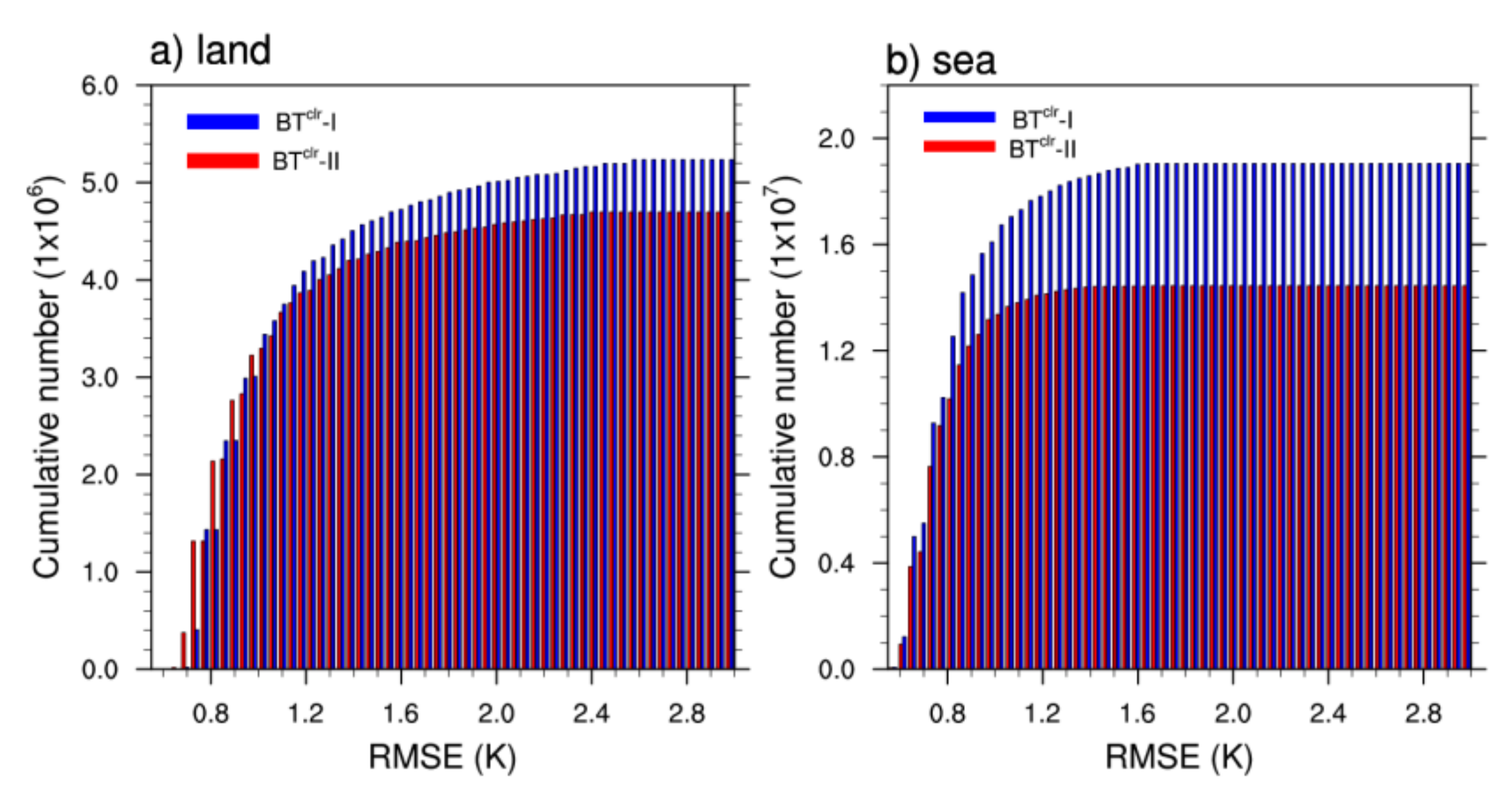
In the superobservation process, taking the ‘probably clear’ pixels as clear, namely use both ‘probably clear’ and ‘clear’ pixels to make BT^clr, actually lower the threshold to make BT^clr comparing to that taking the ‘probably clear’ pixels as cloudy, i.e., only use ‘clear’ pixels to make BT^clr. The former would bring us more FOVs but may degrade the quality of BT^clr comparing to the latter. To determine whether the ‘probably clear’ pixels should be treated as clear or cloudy, we made two kinds of BT^clr, processing the ‘probably clear’ pixels as clear (BT^clr-I) and cloudy (BT^clr-II) respectively. One-month (January of 2019) FOVs of the two kinds of BT^clr were partitioned into different groups according to cloud cover and STD, and the RMSE to background of each group was calculated. Then, the cumulative FOV numbers against the RMSE were counted. The terrestrial and marine results of channel 9 are shown in Figure 1, and the results of channel 10 are similar (not shown). For the FOVs over land, there were more FOVs in BT^clr-II than in BT^clr-I when the RMSE was less than 0.75 K (Figure 1a), meaning BT^clr-II brought us more high-quality observations. In a range of RMSEs between 0.8 K and 1 K, a tiny difference was found between the cumulative FOV numbers of the two cases. The cumulative numbers of BT^clr-I prevailed over BT^clr-II when the RMSE was larger than 1 K and did not change significantly beyond 2 K. Overall, the FOV number of BT^clr-I was about 50,000 more than that of BT^clr-II. This is because BT^clr-I calculate BT at some FOVs that BT^clr-II does not. For example, if a FOV contains 4 ‘probably cloudy’ pixels and 5 ‘probably clear’ pixels. BT^clr-II would take this FOV as totally cloudy and has no value. Whereas BT^clr-I would take this FOV as partially clear and produce a value as the average BT of the 5 ‘probably clear’ pixels. On the other hand, the marine FOV numbers of BT^clr-I were greater than those of BT^clr-II to any RMSE (Figure 1b). Beyond 1.6 K, the numbers became stable, and the FOV number of BT^clr-I was about 500,000 more than that of BT^clr-II in total. In summary, BT^clr-II had more high-quality FOVs over land, but the total FOV numbers were less than BT^clr-I and did not have any advantage over sea. The advantage of BT^clr-II further weakened as we developed a scoring system to filter out high-quality data. Therefore, the ‘probably clear’ pixels were treated as clear in the superobservation process of CSR.d.

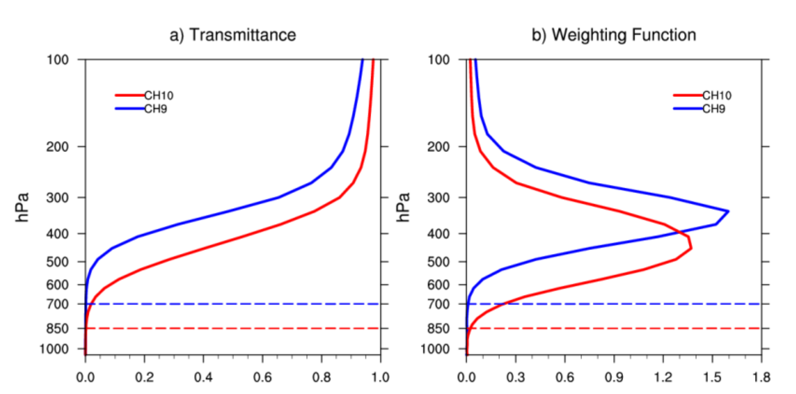
Usually, a weighting function can be used to determine the most sensitive pressure layer in a satellite sounding channel, which can be defined as (7):

$$\begin{array}{c}\mathrm{wf}=\frac{\partial {\tau }_k}{\partial \ln \left(p_k-p_{k+1}\right)}\end{array}$$

(7)

where ${\tau }_k$ is the transmittance between level $p_k$ and level $p_{k+1}$. Layer transmittances of channels 9 and 10 were calculated by RTTOV using a US standard atmosphere profile. The transmittances of the two channels were both close to zero near the surface and increased dramatically in the mid-troposphere (Figure 2a), and the weighting functions peaked at approximately 350 hPa and 450 hPa (Figure 2b). To ensure that the WV-channel observed radiance did not contain too much surface emission, a threshold of height (H_h) was defined at a level at which both the transmittance and its variability were not significantly different from zero, which were 700 hPa and 850 hPa, or approximately 3 km and 1.5 km for channel 9 and channel 10 of the AGRI, respectively.

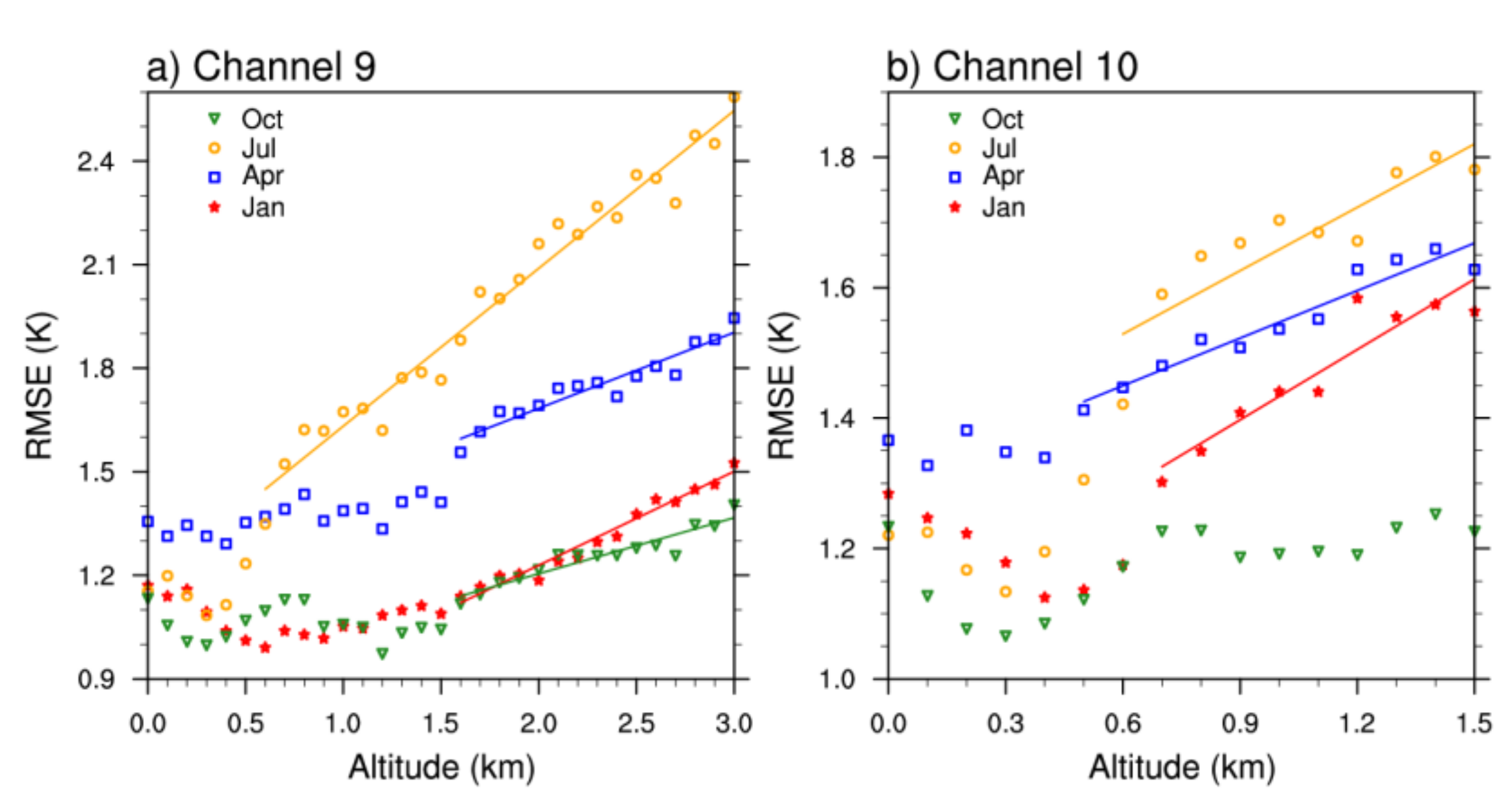
The impact of the altitude on BT^clr quality was explored by examining the relationships between RMSEs and altitude in various months. The altitude was discretized with 100 m intervals from 0 m to H_h. As Figure 3a shows, the RMSE of channel 9 fluctuated by approximately 0.9–1.2 K in January and October and by approximately 1.3–1.5 K in April below 1600 m. Then, RMSE increased almost linearly with different slopes in the three months. However, for RMSE in July, the turning point of RMSE was 1.35 K at 600 m. These phenomena implied that terrain height may not significantly influence BT^clr quality until it reached a certain altitude. Thus, we introduced another height threshold H_l to determine whether we should consider the impact of elevation. H_l could be 1600 m in January, April, and October and 600 m in July for channel 9. Similar results were found for channel 10 (Figure 3b), and the appropriate H_l could be 700 m in January, 500 m in April, and 600 m in July. For October, as the RMSE did not exhibit an increasing trend under 1500 m, we would not consider the impact of altitude. Between H_l and H_h, we linearly fit the relationships between RMSEs and elevation in different months for both channels (solid lines in Figure 3) and used the slopes (parameter ‘l’ in (5)) to represent the influence of altitude.

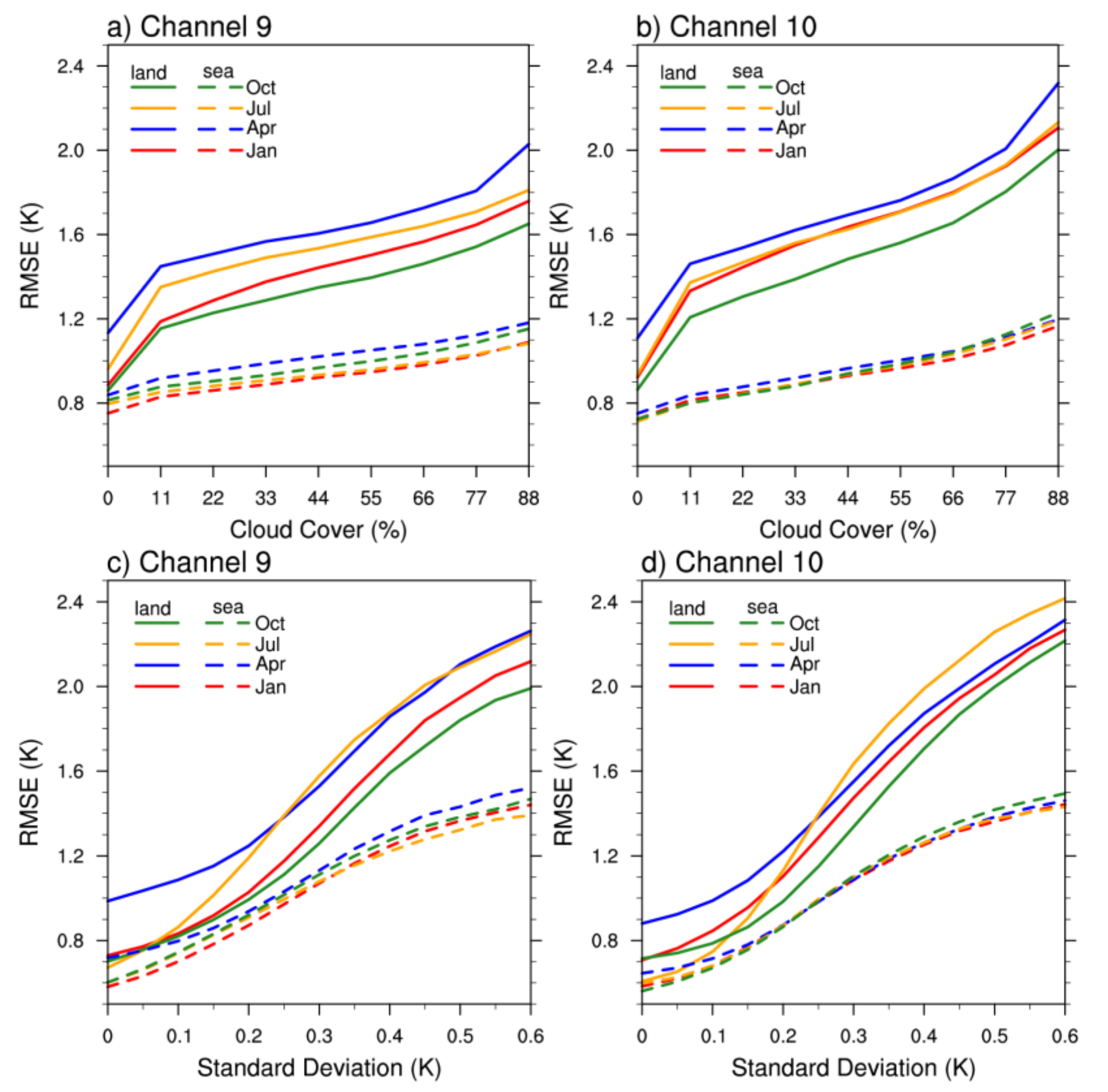
Unlike altitude, cloud cover and STD had robust impacts on the RMSE of BT^clr. The relationships between RMSEs and cloud cover are shown in Figure 4 for the two channels in all four months both over sea and over land with altitudes less than H_l. Both channels suggested that the quality of FOVs over sea was significantly better than that over land. For the channel-9 FOVs over sea, RMSE was approximately 0.8 K in the clear case and grew with a regular slope to 1.1–1.2 K as the cloud cover increase to 88% in the four months (Figure 4a). On the other hand, the RMSE of terrestrial FOVs showed much larger seasonal variation. The RMSE in clear case was 0.85 K in January and October, 0.95 K in July and 1.15 K in April. It increased rapidly to 1.15 K in January and October, to 1.35 K in July and to 1.46 K in April when the cloud cover increased to 11%. Then, the increments of RMSE were approximately 0.5–0.6 K when the cloud cover increased to 88% in all months. Similar results could be obtained for channel 10 in Figure 4b, although with a weaker seasonal variation. The impacts of STD on RMSE were demonstrated using the FOVs with STDs less than 0.6 K, which account for more than 99% total CSR FOVs (Figure 4c,d). Similar to cloud cover, RMSE increased with STD, and the increasing rates were highest between 0.15 K and 0.45 K. A larger RMSE and seasonal variation could be seen for terrestrial FOVs than for marine FOVs for the two channels.

As we had removed the FOVs with sensor zenith angle larger than 60°, more than 50% FOVs were in the regions between 20° S and 20° N. Therefore, the seasonal variation shown in Figure 4 mainly represents the RMSE characteristics of BT^clr in tropical and subtropical regions. We examined the seasonal variation of RMSE in the extratropical northern hemisphere (ENH, north to 20° N), tropical region (TR, between 20° S and 20° N), and extratropical southern hemisphere (ESH, south to 20° S). The results suggested the RMSE characteristics in tropics resemble that in ESH but with larger values (not shown). Comparing to the RMSE in TR, the RMSE in ENH are larger in April and July, whereas they are smaller in October and January. Based on these results, we supposed the representative error introduced by spatial and temporal interpolation when calculating the RMSE would be a key factor affecting the seasonal variation: In tropics and the extratropical regions in summer, there are more mesoscale convection systems and synoptic processes compared to the extratropical regions in winter, which would change the atmospheric WV more rapidly and at a smaller space scale. Thus, there would be larger differences between WV-channel observed BT and NWP simulated BT if their scales are different.

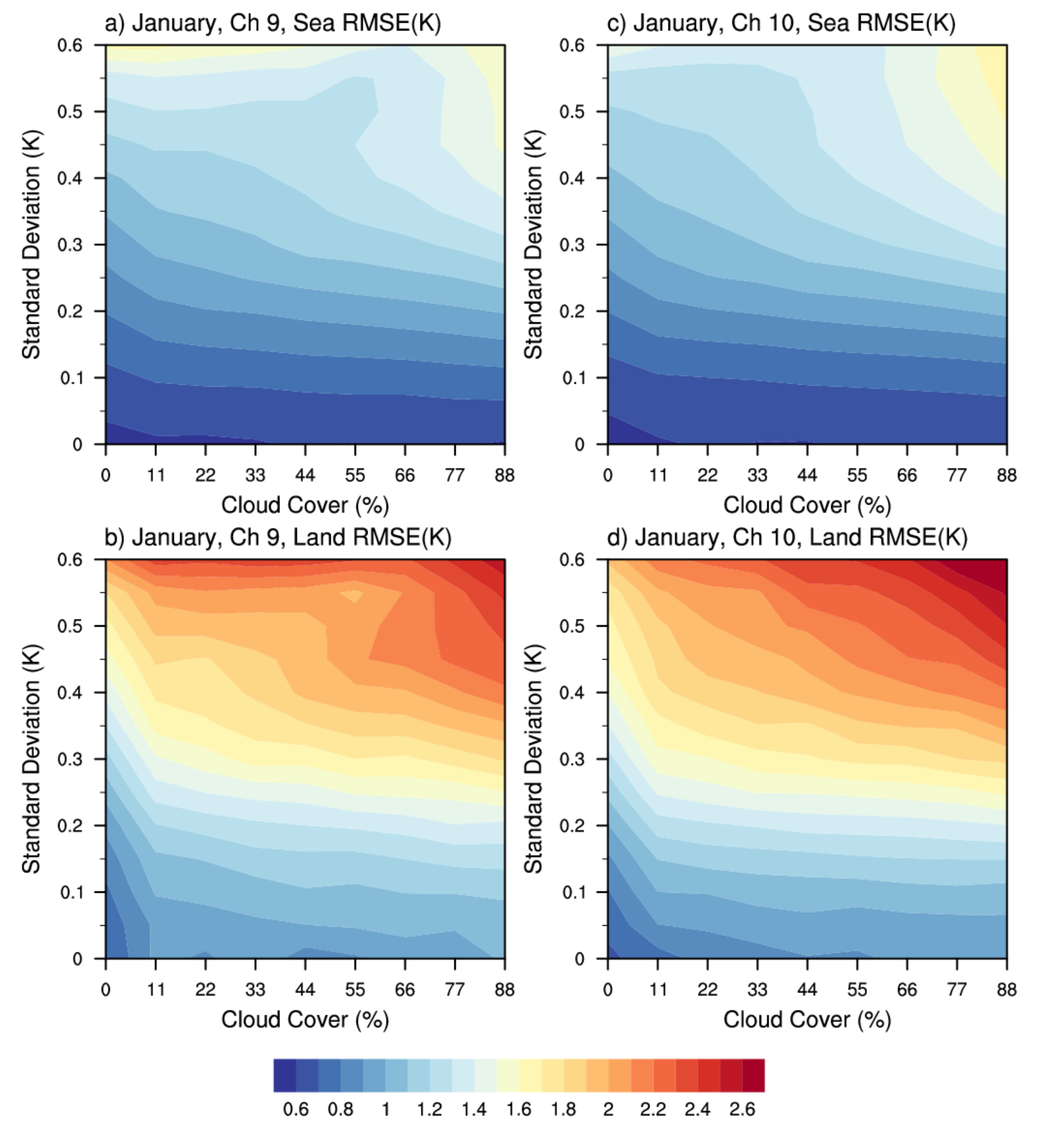
Previous analyses demonstrated RMSE steadily and monotonically increases along with cloud cover and STD. Therefore, we made terrestrial and marine RMSE LUTs in different months taking them as independent variables to predict the RMSE of BT^clr. The LUTs of channel 9 and channel 10 in January are shown in Figure 5. For the marine LUT of channel 9 (Figure 5a), the isolines of RMSE were nearly horizontally distributed when the STD was less than 0.2 K, meaning that the STD was the dominant factor affecting the quality of BT^clr. This result suggested that BT^clr can well represent the BT of the whole FOV despite a high fraction of clouds if the FOV was homogenous enough. As the STD increased, the isolines of RMSE became more slantly distributed, meaning that the influence of cloud coverage increased. The RMSE values with large cloud cover and STD were less reliable since the FOV numbers used to calculate them were small. However, it would not be a problem if the RMSE values exhibit an increasing trend along with the increase of cloud cover and STD. In contrast to the RMSE over sea, the quality of BT^clr over land was much poorer (with a larger RMSE) and more sensitive (with a larger RMSE gradient) to increases in cloud cover and STD (Figure 5b). In addition, cloud cover always played a key role in the BT^clr quality, as the RMSE of all clear FOVs was significantly less than that of FOVs with cloudy pixels. The LUTs of channel 10 resembled those of channel 9 (Figure 5c,d). LUTs in other months were not shown and their main features were similar to the LUTs in January.

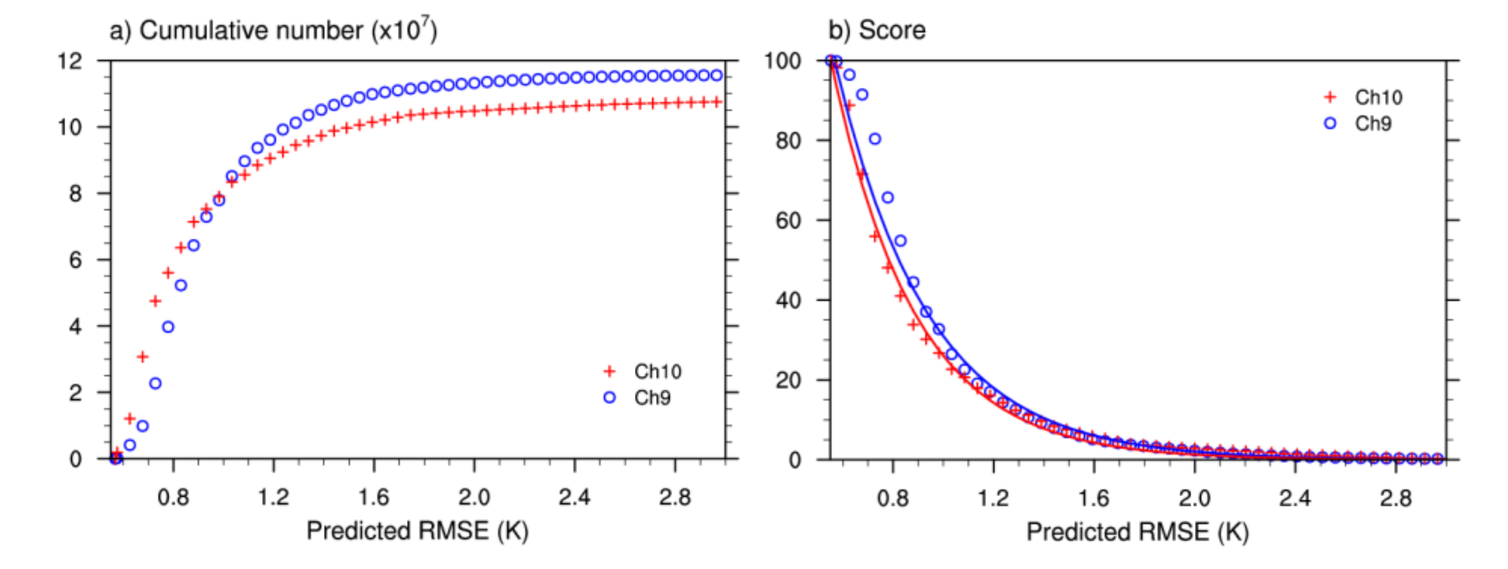
Based on the $RMS{E}_p$, a scoring system was established to indicate the quality of an FOV intuitively. The steps in this process are described as follows: First, equivalent amounts of noncoastal FOVs under H_h were selected from January, April, July and October, and their RMSEs were predicted. Subsequently, the FOVs were ranked according to their $RMS{E}_p$ values. In practice, $RMS{E}_p$ was discretized by a 0.05 K interval, and the cumulative numbers of FOVs were counted. The results of channel 9 and channel 10 are shown in Figure 6a. For both channels, the $RMS{E}_p$ values were no less than 0.55 K. The cumulative numbers grew rapidly between 0.6 K and 1.5 K, meaning that the $RMS{E}_p$ values of most FOVs were in this range. Next, the cumulative numbers were normalized by the total number of FOVs and are denoted by R ranging from 0 to 1. Then, R values were converted to centesimal scores using (8):

$$\begin{array}{c}scor{e}_{LUT}=100-100\times R\end{array}$$

(8)

and the results are LUT scores for $RMS{E}_p$ (dots in Figure 6b). To score the FOVs with continuous $RMS{E}_p$ values, we exploited an exponential decay model to fit the relationship between $RMS{E}_p$ and score in a least squares manner (solid lines in Figure 6b) and derive parameter ‘k’ in (6).

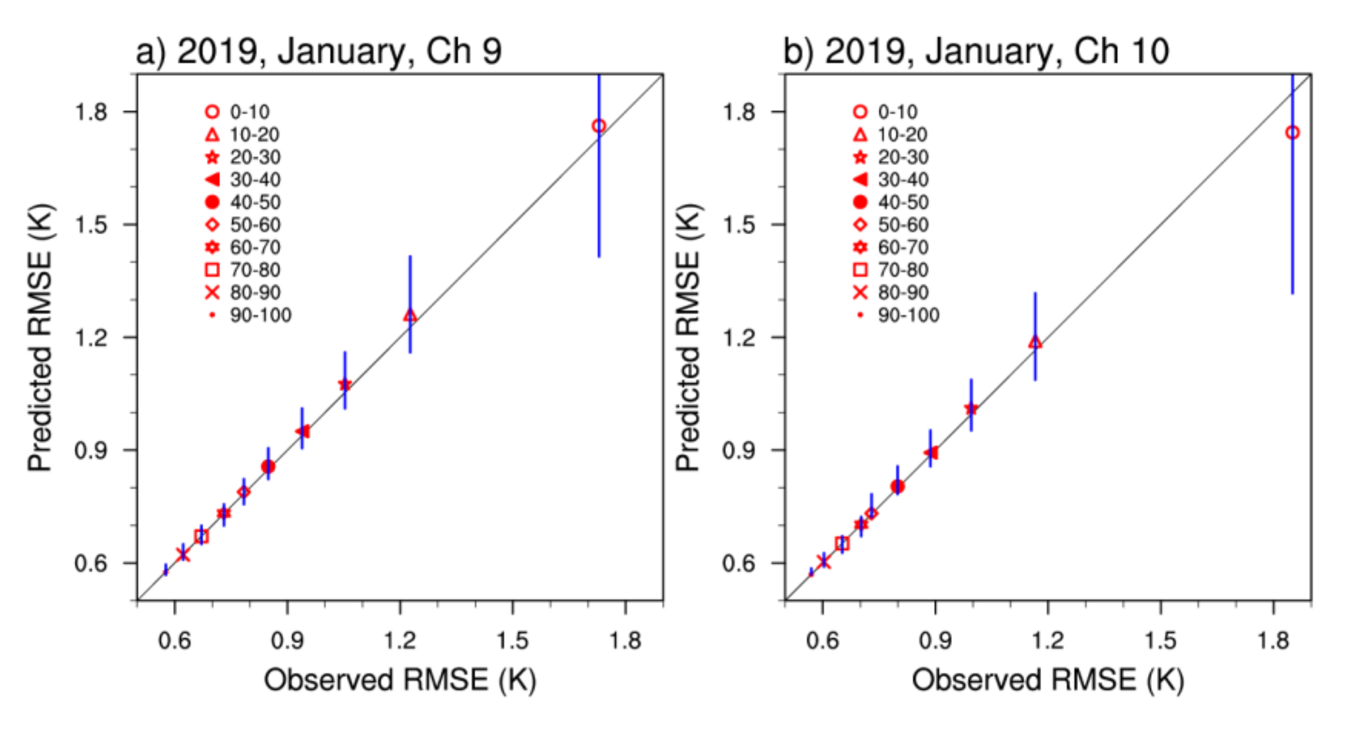
To validate the correctness of the $RMS{E}_p$, we examined the consistency between the observed and predicted RMSEs in different score ranges for both channels. The results of January 2019 are shown in Figure 7, and the same principle could be applied to other months. In this figure, FOVs were partitioned into ten groups according to their score, with ten-point intervals in a left open and right closed manner. The RMSEs of BT^clr and the background fields for each group were calculated, namely, the observed RMSEs, which were taken as independent variables. On the other hand, the $RMS{E}_p$s of all FOVs were taken as dependent variables. The red tabs were the average $RMS{E}_p$s, and the upper and lower blue whiskers indicated the maximum and minimum $RMS{E}_p$s in each group. The average $RMS{E}_p$ values coincided with the observations of both channels for all score groups. However, the $RMS{E}_p$s exhibited a large distribution for low-score FOVs, as the minimum $RMS{E}_p$ for the channel 9 (channel 10) BT^clr under 10 points was 1.41 K (1.26 K), and the maximum reached 2.95 K (3.19 K). As score increased, the dispersion of $RMS{E}_p$ values decreased. For FOVs with scores higher than 90, the difference between the maximum and minimum $RMS{E}_p$s was approximately 0.02 K (0.03 K) for channel 9 (channel 10). In summary, the method in this paper could consistently predict the RMSE of BT^clr, and the score was coherent with the $RMS{E}_p$, especially for FOVs with high scores.

4. Application of CSR Score

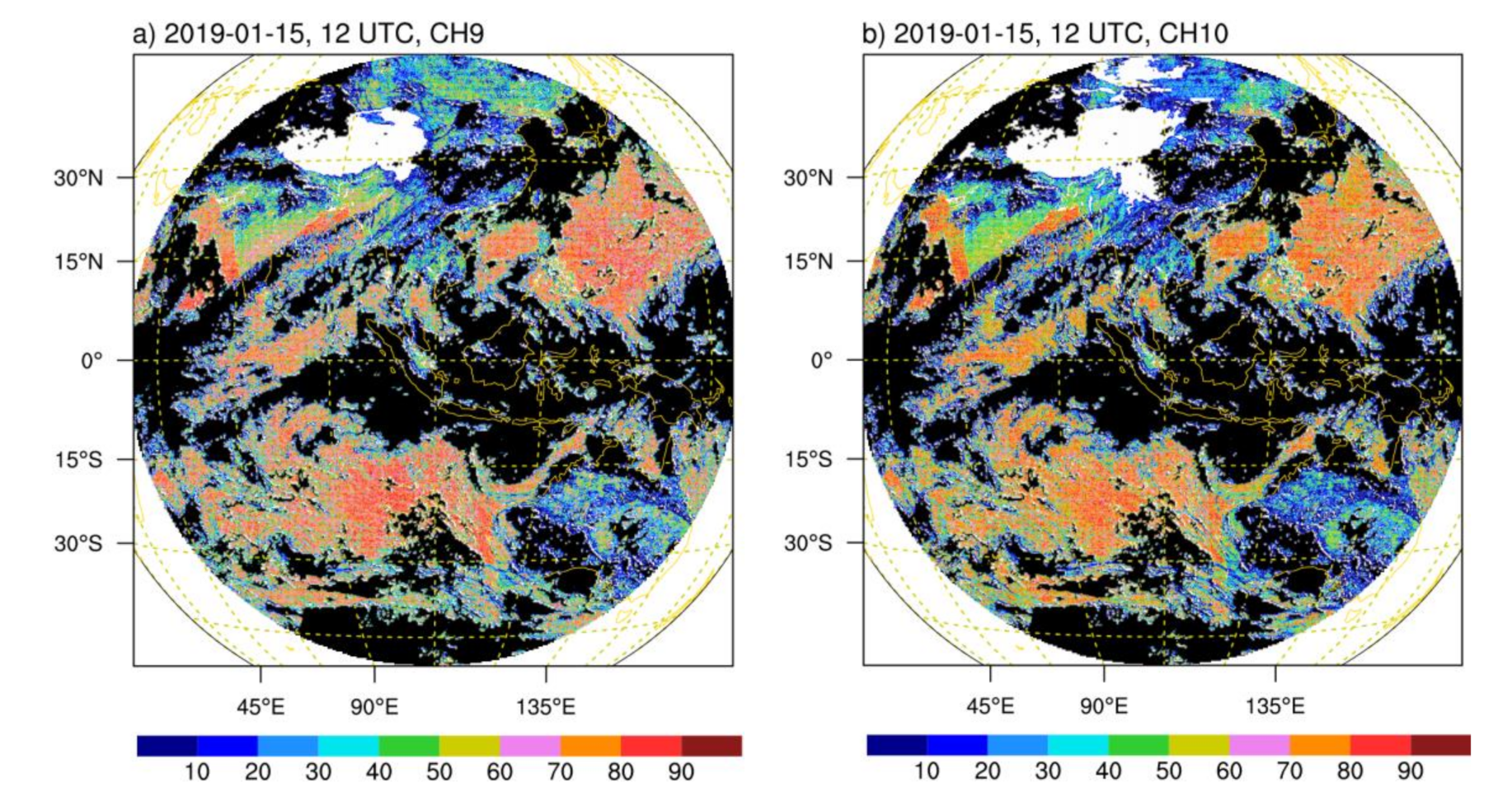
As a demonstration, the BT^clr scores over land and sea with altitudes below H_h are shown in Figure 8 for both channels at 12 UTC on January 15, 2019. The overcast regions derived from cloud fraction product were denoted as black shading. Large areas of clear sky could be found in the Western Pacific and the Southern Indian Ocean. The scores of most FOVs in these areas were higher than 70 points for both channels and decreased to 20–50 points at the edge of the cloud. The impacts of surface type on score were manifested over the clear-sky regions of northern India and the Arabian Sea, where the score changed dramatically across the coast. For channel 9, the scores of the majority of FOVs over northern India were 50–70 points and those over the Arabian Sea were higher than 70 points. By comparison, the score of channel-10 BT^clr was lower over land but higher over sea. When terrestrial FOVs were influenced by cloud, the score would be less than 20 points, such as on the East-Southeast Asian continent and Australia. Moreover, the influence of altitude could be seen by the FOVs around the Tibetan Plateau, especially for channel 9, which was lower than 20 points in a clear situation.

The CSR score ranks the FOVs well according to their quality. However, a threshold is needed to determine whether we should reject an FOV in the QC process. Since CSR was produced to replace L1 data in the data assimilation, the clear-sky L1 data provided a natural reference for setting the threshold. The observed RMSE of BT^clr (RMSE_BT^clr) in each score range spaced by 10 points for channels 9 and 10 are shown in Figure 9, and the lines with various colors represent the observed RMSE to radiance of AGRI pixel (RMSE_L1) under clear skies in January, April, July, and October. For channel 9, the RMSE_L1 was largest in April (1.08 K) and smallest in January (0.76 K), and the averaged value of the four months was 0.90 K. In comparison, the RMSE_BT^clr values under 20 points were larger than the RMSE_L1 in April, the RMSE_BT^clr values above 60 points were smaller than the RMSE_L1 in January, and the RMSE_BT^clr values above 40 points were smaller than the averaged RMSE_L1. Therefore, the quality of CSR above 60 points can be assured, as they were better than the best performance of the L1 data. However, the number of FOVs above 60 points was less than 40% of the total number, and too many FOVs would be discarded if we selected 60 points as the threshold. Therefore, we propose to set the threshold as 40 points, at which the RMSE_BT^clr would be better than the average RMSE_L1 to obtain the balance between amount and quality. For channel 10, the seasonal variation in RMSE_L1 was smaller, with a maximum in April (1.00 K) and a minimum in October (0.75 K), and the average value of the four months was approximately equal to that of channel 9 (0.88 K). The RMSE_BT^clr of channel 10 was similar to channel 9, and above 40 points the RMSE_BT^clr would be significantly less than the average RMSE_L1. Thus, 40 points are proposed as the QC threshold for both channels, which means about 40% data would be discarded in the QC process.

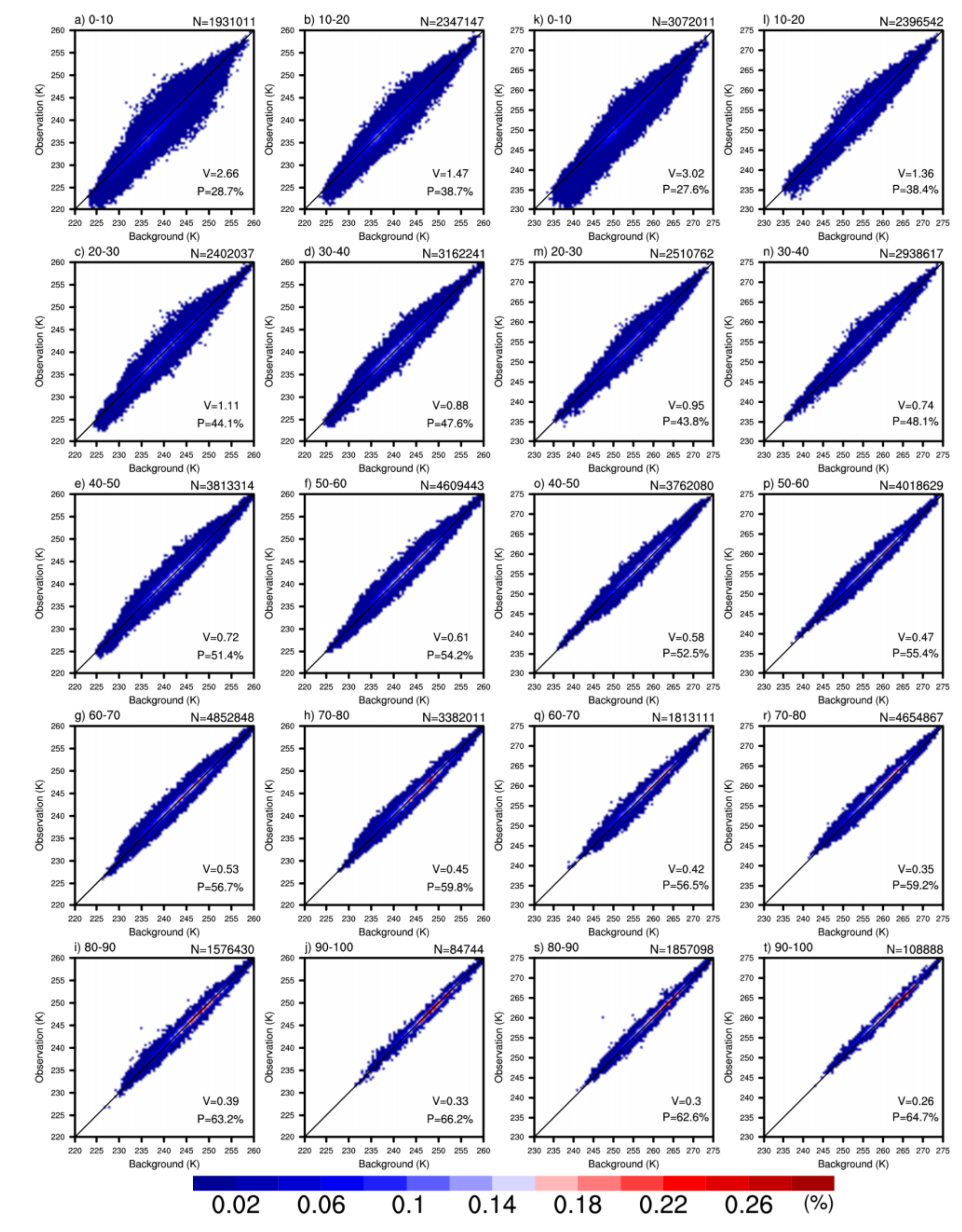
Notably, the score only indicated the quality of BT^clr in a statistical sense. The consistency between observed and background BT^clr in January was examined by their joint probability distributions for both channels, and each is shown in 10 figures with 10-point intervals for the score (Figure 10). The results of other months were similar and not be shown. Low BT (approximately 220 K for channel 9 and 235 K for channel 10) was detected in a score range between 0 and 10, and the lowest BT increased according to the increase in score (approximately 230 K for channel 9 and 240 K for channel 10 in the 90–100 score range). Moreover, the variance in O-B monotonically decreased with increasing score, which was 2.66 K (3.02 K) at a score of 0–10 and 0.33 K (0.26 K) at a score of 90–100 for channel 9 (10). In another way, the probability of small O-B (absolute value < 0.5 K) was calculated to represent the probability of a good BT^clr. The value monotonically increased from 28.7% (27.6%) to 66.2% (64.7%) for channel 9 (10) as the score changed from 10 to 100. When the 40 points that were identified in Figure 9 were used as the QC threshold, the variance of O-B would be less than 0.72 K (0.58 K), and the probability of small O-B would be more than 51.4% (52.5%) for channel 9 (10). It is noted there were some significant outliers in the high-score range (Figure 10i,s). These outliers were over the desert in western and central Australia. In consideration of it is in summer season (January), and the observational BT^clr values are higher than that of background, we believe these outliers were caused by the strong emission of hyperthermal desert surface. These FOVs contaminated by surface emission were scored high because they were all-clear and very homogenous. We could set many criteria to filter out those FOVs and mark them as low score, whereas these outliers were quite easy to remove by setting a threshold on O-B. Our score system was designed to replace the QC of cloud cover and STD of CSR, rather than replace all the QC procedures. Thus, we did not make any corrections for those outliers and suggest using the score and setting a threshold for O-B simultaneously in the QC scheme before assimilation.

5. Discussion

As far as we know, European Organization for the Exploitation of Meteorological Satellites (EUMETSAT) has made a quality index ($QI$) for their CSR product [15]. This index, ranging from 0 to 100, is calculated from two quality indexes based on cloud fraction ($Q{I}_f$) and STD ($Q{I}_{STD}$) as follows:

$$QI=\left(Q{I}_f*Q{I}_{STD}\right)/100$$

(9)

where:

$$Q{I}_f=\left\{{\left[\tan \mathrm{h}\left(\frac{f^{C_f}}{B_f}\right)\right]}^{A_f}\right\}*100$$

(10)

$$Q{I}_{STD}=\left\{{\left[\tan \mathrm{h}\left(\frac{B_{STD}}{ST{D}^{C_{STD}}}\right)\right]}^{A_{STD}}\right\}*100$$

(11)

The tanh function was used because it is monotonic and bounded between 0 and 1 for non-negative values. $A_f$, $B_f$, $C_f$ and $A_{STD}$, $B_{STD}$, $C_{STD}$ are configurable parameters and empirically determined by tuning how quickly the values move from 0 to 1 (personal communication with EUMETSAT user services). The QI has considered the influence of cloud cover and STD on the quality of CSR. In comparison, our scoring system further included the impact of surface type, elevation, and seasonal variation. By using RMSE to indicate the quality of BT^clr, the influence of these factors was evaluated more objectively.

However, we should note that the $RMS{E}_p$ is specific to the background, namely ERA5 reanalysis data in our case. We had taken the background as a reference, but it is not the truth. The error of the background was embedded in the RMSE LUTs so that the $RMS{E}_p$ would change if we use another background. In any case, the RMSE LUTs could reflect how the quality of BT^clr changes along with cloud cover and STD. Therefore, at least the relative quality of BT^clr could be correctly estimated. That is one reason why we convert $RMS{E}_p$ to score to represent the quality of BT^clr in a relative sense. At present, CSR FOVs are assigned the same observation errors in data assimilation, and further improvement is needed to make the observation errors specific [33]. In addition to use for QC, the score may be also used to weight the observation error so that a more accurate assimilation can be achieved, and that will be studied in the future.

References

1. Santurette, P.; Georgiev, C.G. Weather Analysis and Forecasting: Applying Satellite Water Vapor Imagery and Potential Vorticity Analysis, 2nd ed.; Academic Press: New York, NY, USA, 2016; ISBN 9780128001943. [Google Scholar]
2. Velden, C.S.; Hayden, C.M.; Nieman, S.J.; Menzel, W.P.; Wanzong, S.; Goerss, J.S. Upper-Tropospheric Winds Derived from Geostationary Satellite Water Vapor Observations. Bull. Am. Meteorol. Soc. 1997, 78, 173–195. [Google Scholar] [CrossRef] [Green Version]
3. Li, J.; Wang, P.; Han, H.; Li, J.; Zheng, J. On the assimilation of satellite sounder data in cloudy skies in numerical weather prediction models. J. Meteorol. Res. 2016, 30, 169–182. [Google Scholar] [CrossRef]
4. Szyndel, M.D.E.; Kelly, G.; Thépaut, J.N. Evaluation of potential benefit of assimilation of SEVIRI water vapour radiance data from Meteosat-8 into global numerical weather prediction analyses. Atmos. Sci. Lett. 2005, 6, 105–111. [Google Scholar] [CrossRef]
5. Stengel, M.; Unden, P.; Lindskog, M.; Dahlgren, P.; Gustafsson, N.; Bennartz, R. Assimilation of SEVIRI infrared radiances with HIRLAM 4D-Var. Q. J. R. Meteorol. Soc. 2009, 135, 2100–2109. [Google Scholar] [CrossRef]
6. Rani, S.I.; Taylor, R.; Sharma, P.; Bushair, M.T.; Jangid, B.P.; George, J.P.; Rajagopal, E.N. Assimilation of INSAT-3D imager water vapour clear sky brightness temperature in the NCMRWF’s assimilation and forecast system. J. Earth Syst. Sci. 2019, 128, 631. [Google Scholar] [CrossRef] [Green Version]
7. Yang, C.; Liu, Z.; Gao, F.; Childs, P.P.; Min, J. Impact of assimilating GOES imager clear-sky radiance with a rapid refresh assimilation system for convection-permitting forecast over Mexico. J. Geophys. Res. Atmos. 2017, 122, 5472–5490. [Google Scholar] [CrossRef] [Green Version]
8. Zou, X.; Qin, Z.; Weng, F. Improved Coastal Precipitation Forecasts with Direct Assimilation of GOES-11/12 Imager Radiances. Mon. Wea. Rev. 2011, 139, 3711–3729. [Google Scholar] [CrossRef] [Green Version]
9. Qin, Z.; Zou, X.; Weng, F. Evaluating Added Benefits of Assimilating GOES Imager Radiance Data in GSI for Coastal QPFs. Mon. Wea. Rev. 2013, 141, 75–92. [Google Scholar] [CrossRef]
10. Zou, X.; Qin, Z.; Zheng, Y. Improved Tropical Storm Forecasts with GOES-13 / 15 Imager Radiance Assimilation and Asymmetric Vortex Initialization in HWRF. Mon. Wea. Rev. 2015, 143, 2485–2505. [Google Scholar] [CrossRef]
11. Munro, R.; Köpken, C.; Kelly, G.; Thépaut, J.-N.; Saunders, R. Assimilation of Meteosat radiance data within the 4D-Var system at ECMWF: Data quality monitoring, bias correction and single-cycle experiments. Q. J. R. Meteorol. Soc. 2004, 130, 2293–2313. [Google Scholar] [CrossRef]
12. Köpken, C.; Kelly, G.; Thépaut, J.-N. Assimilation of Meteosat radiance data within the 4D-Var system at ECMWF: Assimilation experiments and forecast impact. Q. J. R. Meteorol. Soc. 2004, 130, 2277–2292. [Google Scholar] [CrossRef]
13. Kazumori, M. Satellite Radiance Assimilation in the JMA Operational Mesoscale 4DVAR System. Mon. Wea. Rev. 2014, 142, 1361–1381. [Google Scholar] [CrossRef]
14. Kazumori, M. Assimilation of Himawari-8 Clear Sky Radiance Data in JMA’s Global and Mesoscale NWP Systems. J. Meteorol. Soc. Jap. 2018, 96B, 173–192. [Google Scholar] [CrossRef]
15. EUMETSAT. MSG Meteorological Products Extraction Facility Algorithm Specification Document. EUM/MSG/SPE/022, v7B. 23 October 2015. Available online: https://www-cdn.eumetsat.int/files/2020-04/pdf_msg_met_prod_atbd.pdf (accessed on 12 September 2021).
16. Takahito, I.; Daisaku, U. Clear Sky Radiance (CSR) Product Derived from Himawari-8 Data. Meteorological Satellite Center Technical Note, No. 61. March 2016. Available online: https://www.data.jma.go.jp/mscweb/technotes/msctechrep61-5.pdf (accessed on 12 September 2021).
17. Janjić, T.; Bormann, N.; Bocquet, M.; Carton, J.A.; Cohn, S.E.; Dance, S.L.; Losa, S.N.; Nichols, N.K.; Potthast, R.; Waller, J.A.; et al. On the representation error in data assimilation. Q. J. R. Meteorol. Soc. 2018, 144, 1257–1278. [Google Scholar] [CrossRef]
18. Liu, Z.-Q.; Rabier, F. The interaction between model resolution, observation resolution and observation density in data assimilation: A one-dimensional study. Q. J. R. Meteorol. Soc. 2002, 128, 1367–1386. [Google Scholar] [CrossRef] [Green Version]
19. Ochotta, T.; Gebhardt, C.; Saupe, D.; Wergen, W. Adaptive thinning of atmospheric observations in data assimilation with vector quantization and filtering methods. Q. J. R. Meteorol. Soc. 2005, 131, 3427–3437. [Google Scholar] [CrossRef] [Green Version]
20. Zavodsky, B.; Lazarus, S.; Li, X.; Lueken, M.; Splitt, M.; Ramachandran, R.; Movva, S.; Graves, S.; Lapenta, W. Intelligent Data Thinning Algorithms for Satellite Imagery. In Proceedings of the 2008 IEEE International Geoscience and Remote Sensing Symposium, IGARSS 2008, Boston, MA, USA, 6–11 July 2008; Institute of Electrical and Electronics Engineers: Piscataway, NJ, USA, 2008; Volume 3, pp. 644–647. ISBN 978-1-4244-2807-6. [Google Scholar]
21. Duan, B.; Zhang, W.; Dai, H. ASCAT Wind Superobbing Based on Feature Box. Adv. Meteorol. 2018, 2018, 1–10. [Google Scholar] [CrossRef] [Green Version]
22. Lu, Q.; Hu, J.; Wu, C.; Qi, C.; Wu, S.; Xu, N.; Sun, L.; Li, X.; Liu, H.; Guo, Y.; et al. Monitoring the performance of the Fengyun satellite instruments using radiative transfer models and NWP fields. J. Quant. Spectrosc. Radiat. Transfer. 2020, 255, 107239. [Google Scholar] [CrossRef]
23. Martins, J.V. MODIS Cloud screening for remote sensing of aerosols over oceans using spatial variability. Geophys. Res. Lett. 2002, 29, MOD4-1–MOD4-4. [Google Scholar] [CrossRef] [Green Version]
24. Li, J.; Zou, X. Impact of FY-3A MWTS radiances on prediction in GRAPES with comparison of two quality control schemes. Front. Earth Sci. 2014, 8, 251–263. [Google Scholar] [CrossRef]
25. National Research Council. Four-Dimensional Model Assimilation of Data: A Strategy for the Earth System Sciences; National Academy Press: Washington, DC, USA, 1991; ISBN 0309045363. [Google Scholar]
26. Zhang, P.; Zhu, L.; Tang, S.; Gao, L.; Chen, L.; Zheng, W.; Han, X.; Chen, J.; Shao, J. General Comparison of FY-4A/AGRI With Other GEO/LEO Instruments and Its Potential and Challenges in Non-meteorological Applications. Front. Earth Sci. 2019, 6, 151. [Google Scholar] [CrossRef] [Green Version]
27. Yang, J.; Zhang, Z.; Wei, C.; Lu, F.; Guo, Q. Introducing the New Generation of Chinese Geostationary Weather Satellites, Fengyun-4. Bull. Amer. Meteor. Soc. 2017, 98, 1637–1658. [Google Scholar] [CrossRef]
28. Zhang, P.; Lu, Q.; Hu, X.; Gu, S.; Yang, L.; Min, M.; Chen, L.; Xu, N.; Sun, L.; Bai, W.; et al. Latest Progress of the Chinese Meteorological Satellite Program and Core Data Processing Technologies. Adv. Atmos. Sci. 2019, 36, 1027–1045. [Google Scholar] [CrossRef]
29. Xian, D.; Zhang, P.; Gao, L.; Sun, R.; Zhang, H.; Jia, X. Fengyun Meteorological Satellite Products for Earth System Science Applications. Adv. Atmos. Sci. 2021, 6, 644. [Google Scholar] [CrossRef]
30. Geng, X.; Min, J.; Yang, C.; Wang, Y.; Xu, D. Analysis of FY-4A AGRI bias characteristics and correction experiment. Chin. J. Atmos. Sci. 2019, 44, 679–694. [Google Scholar] [CrossRef]
31. Zhu, J.; Shu, J.; Guo, W. Biases Characteristics Assessment of the Advanced Geosynchronous Radiation Imager (AGRI) Measurement on Board Fengyun–4A Geostationary Satellite. Remote Sens. 2020, 12, 2871. [Google Scholar] [CrossRef]
32. Zhang, L.; Liu, Y.; Liu, Y.; Gong, J.; Lu, H.; Jin, Z.; Tian, W.; Liu, G.; Zhou, B.; Zhao, B. The operational global four-dimensional variational data assimilation system at the China Meteorological Administration. Q. J. R. Meteorol. Soc. 2019, 145, 1882–1896. [Google Scholar] [CrossRef] [Green Version]
33. Burrows, C. Assimilation of Radiance Observations from Geostationary Satellites: Second Year Report, EUMETSAT/ECMWF Fellowship Programme Research Report; ECMWF: Reading, UK, 2019. [Google Scholar]
34. Saunders, R.; Hocking, J.; Turner, E.; Rayer, P.; Rundle, D.; Brunel, P.; Vidot, J.; Roquet, P.; Matricardi, M.; Geer, A.; et al. An update on the RTTOV fast radiative transfer model (currently at version 12). Geosci. Model Dev. 2018, 11, 2717–2737. [Google Scholar] [CrossRef] [Green Version]
35. Hersbach, H.; Bell, B.; Berrisford, P.; Hirahara, S.; Horányi, A.; Muñoz-Sabater, J.; Nicolas, J.; Peubey, C.; Radu, R.; Schepers, D.; et al. The ERA5 global reanalysis. Q. J. R. Meteorol. Soc. 2020, 146, 1999–2049. [Google Scholar] [CrossRef]
Figure 1. (a) Terrestrial and (b) marine cumulative numbers of channel-9 BTclr-I (considering ‘probably clear’ pixels to be clear) and BTclr-II (considering ‘probably clear’ pixels to be cloudy) against RMSE.
Remotesensing 13 03658 g001
Figure 2. (a) Layer transmittances from different pressure levels to the top of the atmosphere and (b) the weighting function for channels 9 and 10 of the AGRI.
Remotesensing 13 03658 g002
Figure 3. Relationships between RMSE and altitude for (a) channel 9 and (b) channel 10 in January, April, July, and October (markers). Solid lines are the linear fitting of the relationships from altitude Hl to Hh.
Remotesensing 13 03658 g003
Figure 4. Relationships between RMSE and cloud cover for (a) channel 9 and (b) channel 10 in January, April, July and October. Different colors are used for different months, and solid (dashed) lines are used for terrestrial (marine) FOVs. (c,d) are the same as (a,b) but for the relationship between RMSE and STD.
Remotesensing 13 03658 g004
Figure 5. (a) Marine and (b) terrestrial RMSE lookup table of channel 9 in January. (c,d) are the same as (a,b) but for channel 10.
Remotesensing 13 03658 g005
Figure 6. (a) Cumulative histogram of the FOV number and (b) resulting score (dots) against RMSE for channel 9 and channel 10. The curves in (b) fit the relationship between the score and RMSE using the exponential decay model.
Remotesensing 13 03658 g006
Figure 7. Average values (red markers) of the predicted RMSE against the observed RMSE in each BTclr group partitioned by 10-point intervals for (a) channel 9 and (b) channel 10 in January 2019. The upper and lower limits of predicted RMSE in each score range are denoted as blue whiskers.
Remotesensing 13 03658 g007
Figure 8. The scores of (a) channel 9 and (b) channel 10 BTclr at 12 UTC on 15 January 2019. Overcast regions were denoted as black shading.
Remotesensing 13 03658 g008
Figure 9. RMSEs in different score ranges for (a) channel 9 and (b) channel 10. The dotted lines of different colors are the RMSE of clear-sky L1 data for backgrounds in different months, and the average RMSE of the four months is denoted as a black solid line.
Remotesensing 13 03658 g009
Figure 10. (aj) are joint probability distributions (in percent) of channel 9 BTclr and background BT in different score ranges for January, 2019. The score range, FOV numbers (denoted as N), variance in O-B (denoted as V) and the probability of O-B in the range of -0.5 K to 0.5 K (denoted as P) are labeled at the top left, top right and bottom right, respectively, in each subfigure. (kt) are the same as (aj) but for channel 10. Totally, more than 28 (27) million FOVs were used for channel 9 (10).
Remotesensing 13 03658 g010
Publisher’s Note: MDPI stays neutral with regard to jurisdictional claims in published maps and institutional affiliations.