Article

Applications of the Advanced Radiative Transfer Modeling System (ARMS) to Characterize the Performance of Fengyun–4A/AGRI

1
Key Laboratory of Transportation Meteorology, China Meteorological Administration, Nanjing 210041, China
2
Nanjing Joint Institute for Atmospheric Sciences, Nanjing 210041, China
3
State Key Laboratory of Severe Weather, Chinese Academy of Meteorological Sciences, Beijing 100081, China
4
National Satellite Meteorological Center, Beijing 100081, China
*
Author to whom correspondence should be addressed.
Remote Sens. 2021, 13(16), 3120; https://doi.org/10.3390/rs13163120
Submission received: 14 May 2021 / Revised: 27 July 2021 / Accepted: 3 August 2021 / Published: 6 August 2021
(This article belongs to the Special Issue Remote Sensing of Clouds and Precipitation at Multiple Scales)

Abstract

:
This study applies the Advanced Radiative Transfer Modeling System (ARMS), which was developed to accelerate the uses of Fengyun satellite data in weather, climate, and environmental applications in China, to characterize the biases of seven infrared (IR) bands of the Advanced Geosynchronous Radiation Imager (AGRI) onboard the Chinese geostationary meteorological satellite, Fengyun–4A. The AGRI data are quality controlled to eliminate the observations affected by clouds and contaminated by stray lights during the mid–night from 1600 to 1800 UTC during spring and autumn. The mean biases, computed from AGRI IR observations and ARMS simulations from the National Center for Environmental Prediction (NCEP) Final analysis data (FNL) as input, are within −0.7–1.1 K (0.12–0.75 K) for all seven IR bands over the oceans (land) under clear–sky conditions. The biases show seasonal variation in spatial distributions at bands 11–13, as well as a strong dependence on scene temperatures at bands 8–14 and on satellite zenith angles at absorption bands 9, 10, and 14. The discrepancies between biases estimated using FNL and the European Center for Medium–Range Weather Forecasts Reanalysis–5 (ERA5) are also discussed. The biases from water vapor absorption bands 9 and 10, estimated using ERA5 over ocean, are smaller than those from FNL. Such discrepancies arise from the fact that the FNL data are colder (wetter) than the ERA5 in the middle troposphere (upper–troposphere).

1. Introduction

As the first of China’s new-generation geostationary meteorological satellites, Fengyun (FY) –4A was launched on 11 December 2016. The main imager instrument onboard FY-4A is the Advanced Geosynchronous Radiation Imager (AGRI). It has fourteen bands, including eight infrared (IR), two visible, and four near-IR bands. The AGRI is very similar to the Advanced Himawari Imager (AHI) onboard the Japanese geostationary meteorological satellites Himawari–8 and –9 [1], and the Advanced Baseline Imager (ABI) onboard the U.S. Geostationary Operational Environmental Satellite (GOES)–R series [2]. These new–generation geosynchronous imagers are important for numerical data assimilation and weather forecasting [3,4,5,6,7], disaster prevention and mitigation [8,9], as well as atmosphere and surface parameter retrievals [10,11,12,13].
In atmospheric parameter retrievals and numerical data assimilations, it is important to characterize the biases of the measurements with respect to “truth” data. Two common approaches are used to quantify the biases of a geosynchronous imager. The first one performs intercomparisons of radiance observations with the multispectral imagers or hyperspectral infrared sounders onboard other geostationary or polar–orbiting meteorological satellites [14]. This approach is applicable in any sky conditions and for any surface type. However, the intercomparison is limited to equatorial regions in which the coincident, co–angled, and collocated measurements can be found [15]. Another way is to compare observations to the radiative transfer model simulations from Numerical Weather Prediction (NWP) fields as inputs. This Observation Minus Background–simulation (OMB) approach is applicable over the full–disk observations under clear–sky conditions. It is worth mentioning that the OMB statistics include not only the instrumental observation errors, but also the systematic errors in a radiative transfer model and an NWP field [16]. However, it is not crucial to separate the radiative transfer model bias from the observation bias, since it is their sum that is required for radiance data assimilation [17,18].
An accurate and fast radiative transfer model is required in the OMB approach. Currently, the most widely used fast radiative transfer models for satellite data applications are the Radiative Transfer for TIROS Operational Vertical Sounder (RTTOV) [19,20] and the Community Radiative Transfer Model (CRTM) [21,22]. Zou et al. [23] analyzed the bias characteristics of Himawari–8/AHI IR bands using two radiative transfer models (the CRTM and RTTOV) and compared the bias results obtained from the simulations of both models. Their work on bias estimation has facilitated the use of AHI in data assimilation [7,24,25,26]. For FY–4A/AGRI, three existing studies have contributed to its IR band biases using the OMB approach [27,28,29]. Qu et al. [27] used ECMWF Reanalysis–5 (ERA5) data as input to the RTTOV model in order to calculate and analyze the biases of the AGRI seven 4 km–resolution IR bands. Geng et al. [28] also employed RTTOV, but they used Global Forecast System (GFS) analysis data as input. They incorporated a variational bias correction scheme for the future application of AGRI data in the Weather Reacher and Forecasting Data Assimilation (WRFDA). Zhu et al. [29] coupled the RTTOV and ERA5 to evaluate the AGRI IR bands’ bias over its full–disk.
In parallel with the rapid development of Chinese geostationary and polar-orbit meteorological satellites (also known as FY–series satellites), the Advanced Radiative Transfer Modeling System (ARMS) was also developed by China’s Meteorological Administration (CMA). ARMS can now simulate the radiances observed by various spaceborne instruments in IR and microwave spectrum under different atmospheric and surface conditions. The ARMS version 1.0 is expected to be released to the public soon. Preliminary test results obtained by Yang et al. (2020) have shown that ARMS’s performance is very reliable in terms of its accuracy and precision [30,31].
ARMS has improved upon CRTM and RTTOV in both scientific and software aspects. For the radiative transfer model solvers in ARMS, both the polarized two–stream model [32] and the scalar Discrete Ordinate Adding Method [33] are used as standard solvers in addition to some advanced radiative transfer schemes, such as the advanced doubling–adding (ADA) method [34], Vector Doubling–Adding method [35], and the vector discrete–ordinate radiative transfer model [36,37,38]. The abovementioned two solvers are designed for simulating in ultraviolet to visible wavelengths, where it is possible for scattering from molecules and aerosols to exhibit high anisotropic behaviors and where more accurate streams in the radiative transfer simulations are required [30]. However, CRTM and RTTOV employed the ADA and delta-Eddington approximation methods [39] as their main drivers, respectively, and these can only handle the polarized signals generated by the surfaces and not the polarization related to the scattering of clouds and aerosol particles [30]. For particle absorption and scattering, a super spheroidal model was implemented in ARMS. It has the advantage of generating a lookup table for the fast calculation of aerosols [30]. The ARMS model uses a fast gaseous absorption approach that is similar to Optical Path TRANsmittance [40]. In this approach, the monochromatic atmospheric transmittance is calculated based on the European Center for Medium–Range Weather Forecasts (ECMWF)–83 training profiles and the latest HIgh-resolution TRANsmission molecular absorption database [41]. The Line By Line Radiative Transfer Model [42,43] is used for the calculation of visible and infrared spectrum, while the Monochromatic Radiative Transfer Model [43] is applied for the microwave spectrum. After convolving with the instrumental Spectral Response Function, the band–averaged atmospheric transmittance can be obtained [20]. Then, the clear–sky radiance received at the Top of Atmosphere is simulated. The cloudy radiance simulation additionally requires the vertical profiles of hydrometeor variables, such as the liquid water path, ice water path, and effective radius. Six hydrometeors (e.g., cloud, rain water, cloud ice, snow, graupel, and hail) can be considered in ARMS. Further details about ARMS can be found in References [30,31,33].
To date, no publications have been concerned with the use of ARMS to evaluate the biases of satellite remote-sensing observations. The bias characteristics of AGRI IR bands derived from a radiative transfer model other than RTTOV, such as ARMS, have not been investigated so far. In addition, the existing three efforts on AGRI biases [27,28,29] used only one type of reanalysis or analysis information as input to the radiative transfer models. However, the difference in AGRI bias results caused by different NWP background fields is not clear. In this study, ARMS is applied for the first time to the OMB approach in order to characterize the bias of FY–4A/AGRI IR bands 8–14. The National Center for Environmental Prediction (NCEP) Final analysis data (FNL) is used as input to the ARMS model to generate AGRI radiance simulations. Differences of biases based on FNL and ERA5 are also discussed in this study.
This paper is organized as follows: Section 2 introduces the instrument characteristics of AGRI. The observation anomalies of AGRI band 8 are also analyzed in this section. Section 3 introduces the requirements of the ARMS simulations, including the NWP background datasets, surface emissivity model, and the quality control method for removing cloud-affected radiance data. Section 4 verifies the performance of the ARMS simulation, and biases calculated by ARMS are compared with those calculated by RTTOV. Section 5 presents the biases and standard deviations of OMB differences for seven AGRI IR bands, the seasonal characteristics of biases, and their dependence on scene brightness temperatures and satellite zenith angles. Discussions of discrepancy in biases estimated using FNL and ERA5 background datasets as inputs to ARMS are given in Section 6. Conclusions are provided in Section 7.

2. AGRI Observations

2.1. FY–4A/AGRI Characteristics

The FY–4A satellite adopts a three–axis stabilized attitude control, which can significantly improve the efficiency of Earth observations compared with a spin–stabilized platform. Currently, it is located 35,786 km above the equator, at 104.7°E. AGRI, onboard the FY–4A satellite, has a total of 14 bands, including two visible, four near-IR, and eight IR. It provides a full–disk observation with an interval of 15 min. The nadir spatial resolutions are 0.5 km for the AGRI 0.65 μm band; 1 km for 0.47 and 0.83 μm bands; and 2 km for the 1.378, 1.61, and 2.23 μm bands and the high–resolution 3.75 μm band. For the low–resolution 3.75 μm and the remaining IR bands, the AGRI observation resolution is 4 km. These multiband data can be directly used for the assimilation and retrieval of parameters based on band differences [44]. Table 1 gives the characteristics of AGRI IR bands such as the central wavelengths and spatial resolutions. Note that this study only focuses on the bias characteristics of AGRI IR bands 8–14 over the full–disk domain.
Figure 1 shows the weighting functions of AGRI bands 8–14, calculated using ARMS with the US 1976 standard atmosphere as the input. Among these seven AGRI IR bands, bands 8, 11, 12, and 13 are surface–sensitive. AGRI bands 9 and 10 are located in a water vapor absorption band and, thus, the observations of AGRI bands 9 and 10 are sensitive to water vapor in the troposphere with peak weighting located at 350 hPa and 500 hPa, respectively. AGRI band 14 resides in a carbon dioxide absorption band.
The FY–4A/AGRI data are provided by the National Satellite Meteorological Center of the China Meteorological Administration. The data are in hdf5 format, which is a preprocessed product obtained from AGRI Level 0 source package data after a quality check, and geolocation and radiometric calibration processing. For the full–disk data with a spatial resolution at 4 km, there are always 2748 scan lines, with 2748 scan pixels on each scan line.

2.2. Anomalies of AGRI Brightness Temperature at Band 8

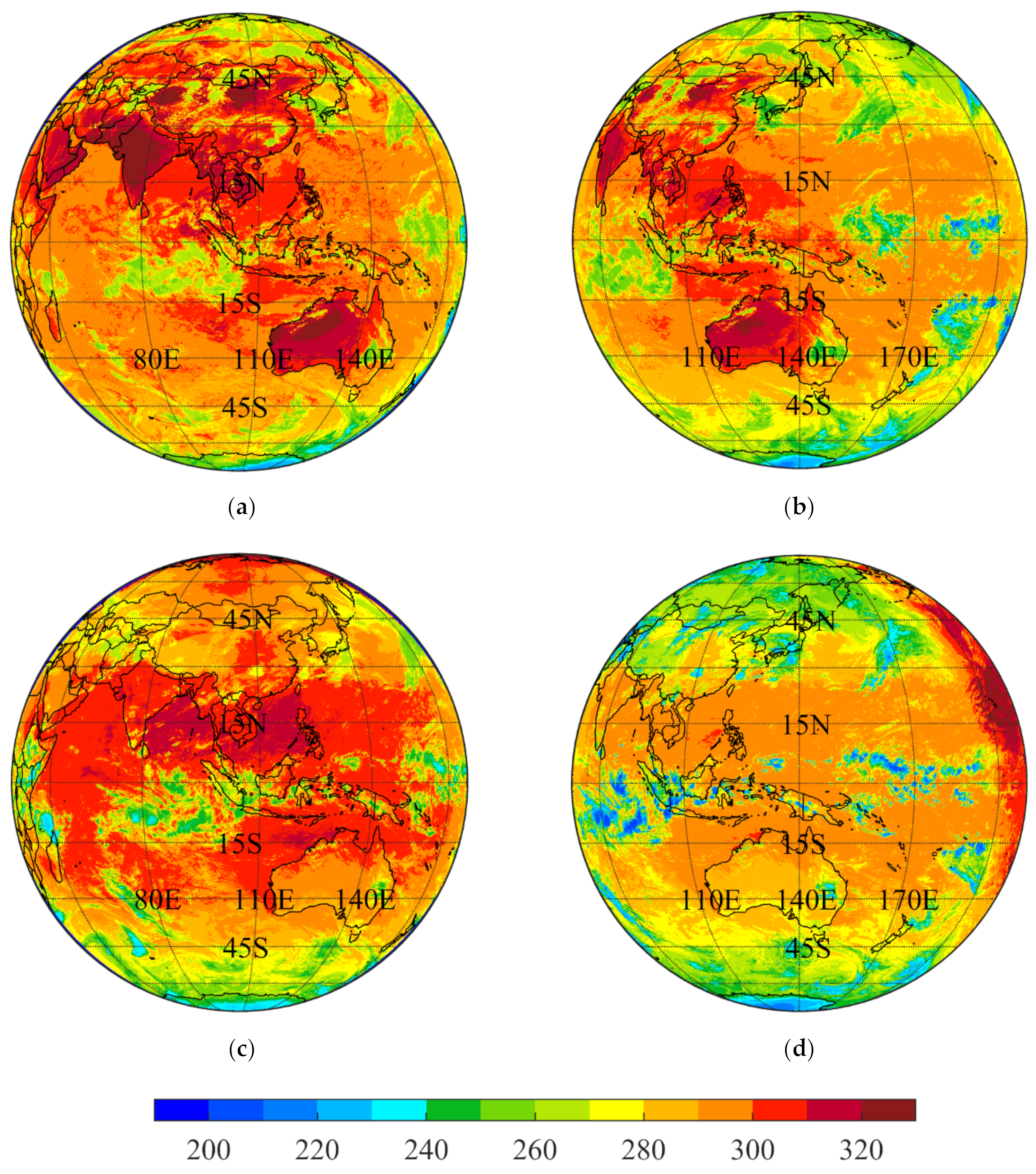
After our diagnoses of AGRI data, AGRI band 8 was found to have some outstanding anomalies around the mid–night hours, which has a serious impact on its bias estimation. However, this problem has not been paid attention by existing literatures. Figure 2 shows the brightness temperatures of both AGRI and AHI at the ~3.75 μm band at 0600 and 1700 UTC on 23 April 2019. It can be seen that, at 0600 UTC, which is during daytime, the AGRI and AHI brightness temperatures in the overlapping region agree well except for clouds, where the AGRI brightness temperatures are slightly higher than those of AHI. However, in the mid–night hours around 1700 UTC, the AGRI brightness temperatures are about 10–20 K higher than the AHI brightness temperatures in both cloudy and clear–sky areas, regardless of whether they are over oceans or over land. For bands 9–14 of AGRI, the observations are generally in reasonable ranges at the high–temperature end when compared with their AHI counterparts (figures omitted).
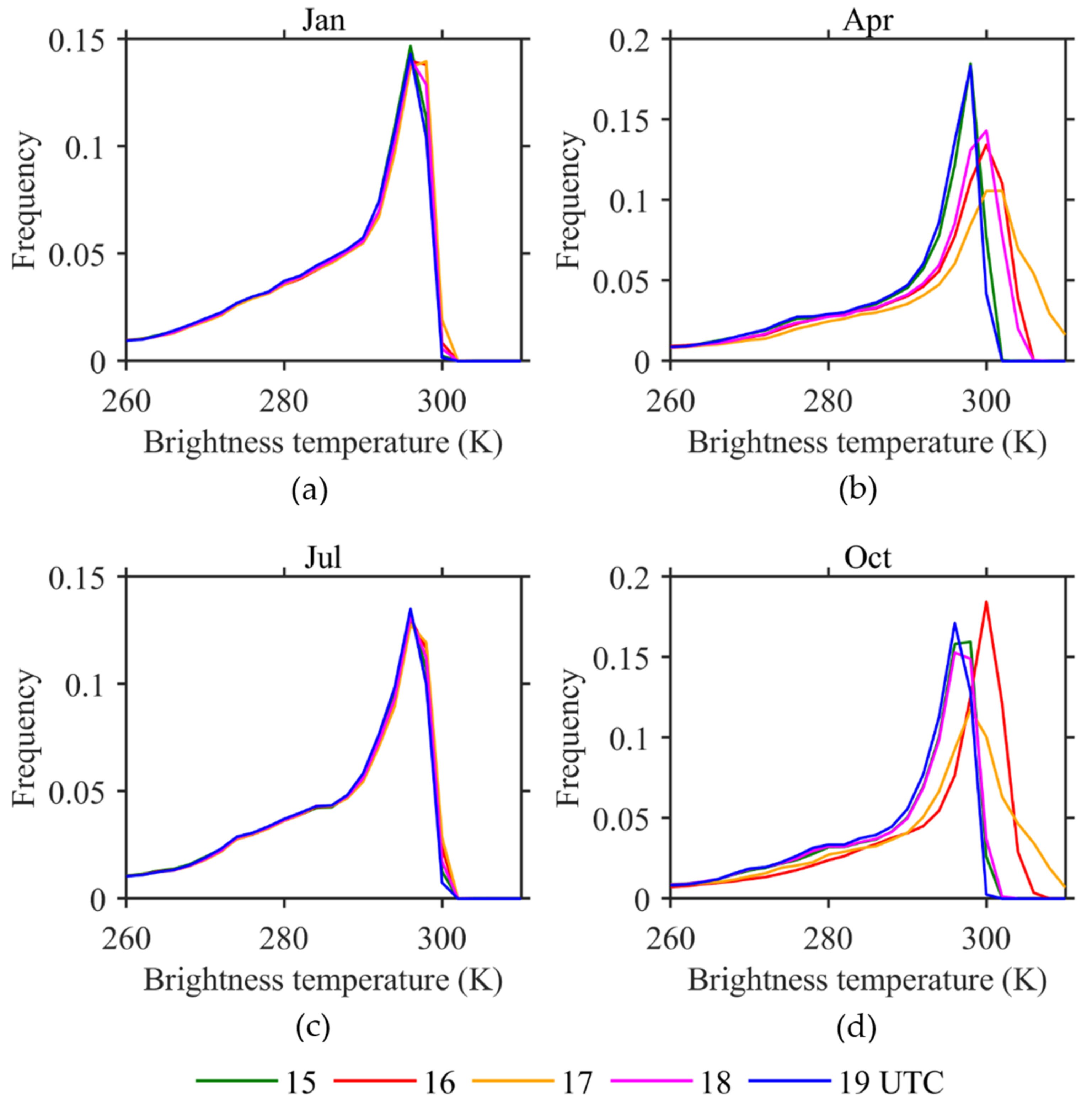
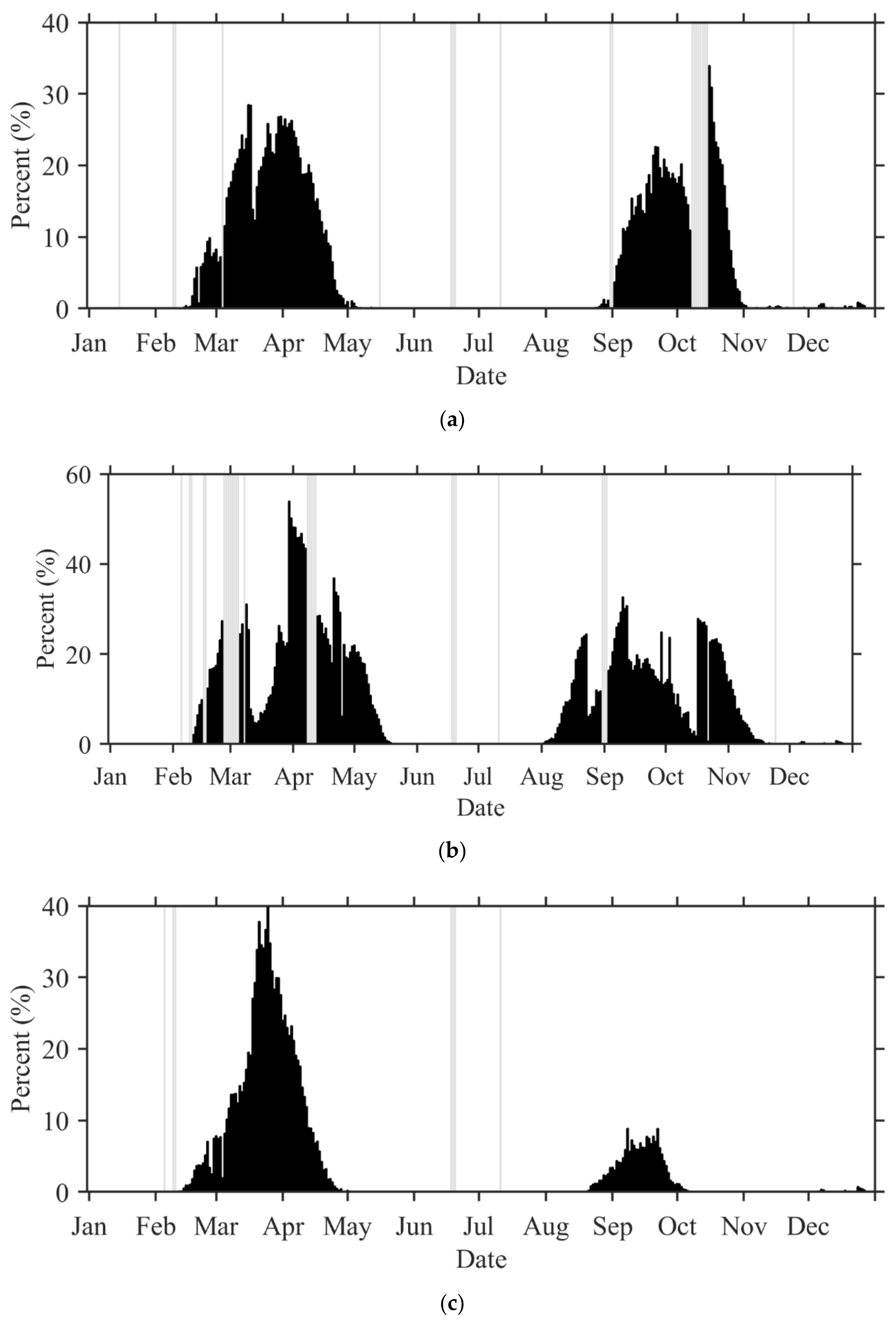
In order to further analyze the temporal characteristics of the observation anomalies in AGRI band 8, the frequency of the brightness temperature values of band 8 at 2 K–intervals was counted by selecting the observations at 1500, 1600, 1700, 1800, and 1900 UTC in January, April, July, and October 2019, respectively, as shown in Figure 3. It can be seen that the brightness temperatures for all five hours in January and July are distributed in a range of less than 300 K (Figure 3a,c). In April, the brightness temperature values at 1500 and 1900 UTC were distributed in a range of less than 300 K, while at 1600, 1700, and 1800 UTC, the brightness temperature distributions shifted to the right with maximum values greater than 310 K (Figure 3b). A similar feature was found in the brightness temperature distributions in October (Figure 3d). This suggests that the brightness temperature anomaly at band 8 had a seasonal dependence during mid–night hours, from 0000 to 0200 local solar time (LST) (i.e., 1600–1800 UTC). To demonstrate this, the number of brightness temperature values for AGRI band 8 above 300 K at 1600, 1700, and 1800 UTC for each day, as a proportion of the total number of observations at that time (i.e., the anomaly proportion), were calculated, and the time series of the anomaly proportion in 2019 were shown in Figure 4. It was found that the anomalies at all these three hours occurred during the 1–2 month period before and after the vernal or autumnal equinoxes. The anomalies at 1700 UTC lasted longer than those during the other two hours. The anomalies at 1700 UTC started from early February and early August, respectively, and ended in mid-May and mid-November, whereas the anomalies at 1600 and 1800 UTC started later than those at 1700 UTC, but ended earlier. The cause of this brightness temperature anomaly in AGRI band 8 is unclear. One possible reason is the contamination of the 3.75 μm band by stray light at midnight, a problem that was reported in relation to the predecessor of FY–4A, namely, the FY–2 series satellites [45].
In this study, when assessing the accuracy of AGRI bands using ARMS, all band data at the hours when the band–8 observations had anomalies are excluded from our statistics.

3. Simulation of AGRI IR Measurements

The AGRI brightness temperature observations of seven, 4 km–resolution IR bands (bands 8–14) under clear–sky conditions were simulated using ARMS version 1.0 or RTTOV version 12.3, with the profiles of atmospheric temperature, water vapor, ozone, and carbon dioxide, as well as surface skin temperature, surface emissivity, and surface wind (both speed and direction) as inputs. A summary of the input variables and parameters used to generate clear–sky radiance simulations is provided in Table 2.

3.1. NWP Background Dataset

Atmospheric three–dimensional variables of pressure, temperature, water vapor, and ozone mixing ratio, and surface two–dimensional variables of skin temperature and surface wind were obtained from ERA5 and FNL, with a resolution of a 0.25° × 0.25° grid at 0000, 0600, 1200, and 1800 UTC. The ERA5 and FNL data had 37 and 31 pressure levels in the vertical direction, respectively. The ozone (water vapor) profile below the 400–hPa height (below the 100–hPa height) was not provided in the FNL dataset. Therefore, when dealing with FNL data, the ozone mixing ratio value at 400–hPa level was used for a level below the 400–hPa height and the water vapor mixing ratio at 100 hPa level was used for levels above the 100–hPa height.

3.2. Infrared Surface Emissivity Dataset

ARMS integrates a series of infrared surface emissivity modules that can handle different surface types including land, ocean, ice, and snow. It also provides an option to allow users to enter their own emissivity spectra. Zhuge et al. [47] demonstrated that the Combined Advanced Spaceborne Thermal Emission and Reflection Radiometer (ASTER) and Moderate Resolution Imaging Spectroradiometer (MODIS) Emissivity over Land (CAMEL) High Spectral Resolution Emissivity dataset (CAMEL_HSRemis) [48] has the highest accuracy, especially over the desert, when compared with other infrared land surface emissivity datasets that are currently available. Therefore, the CAMEL_HSRemis was incorporated into the ARMS simulations as the source of infrared land surface emissivity in this study. The infrared sea surface emissivity was calculated based on the algorithm proposed by Wu and Smith (1997) [46]. Similar approach was used when generating RTTOV simulations.

3.3. Cloud Detection

Since we only evaluated AGRI observational biases under clear–sky conditions, cloud detection was needed before comparing the observations with the model simulations. In this study, the official AGRI cloud products were not used since they were still subject to some errors and uncertainties [49]. Instead, the MODIS cloud mask product (known as MOD35 for Terra satellite and MYD35 for Aqua satellite, hereafter MOD35 for simplicity) of Collection 6 [50] was employed to identify AGRI clear–sky pixels. It has four categories: cloudy, probably cloudy, probably clear, and clear. MOD35 product data were provided by the National Aeronautics and Space Administration.
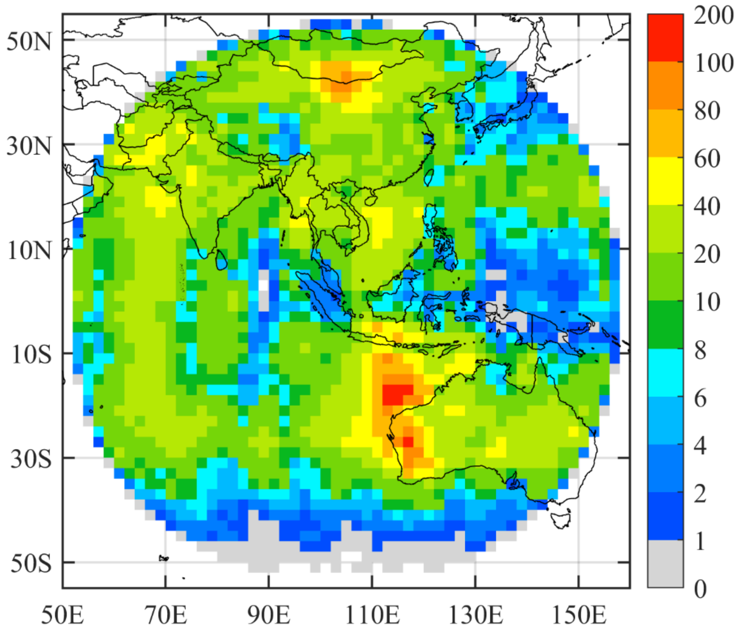
The AGRI and MOD35 data in January, April, July, and October 2019, were selected for seasonal biases analysis. Since MODIS onboard Terra and Aqua satellites observed the Earth at the local times of mid–morning and early afternoon, respectively, the data must be collocated with the FY–4A/AGRI satellite observations. In doing so, the data from Aqua or Terra passing over the AGRI full–disk observation area within 15 min were matched to AGRI observation pixels. If there were probably cloudy, cloudy, or probably clear pixels from the MODIS cloud product found within an AGRI pixel of 4 km, then that AGRI pixel was regarded as cloud–contaminated and excluded from the statistics sample. The total data counts of clear–sky AGRI pixels within 2° × 2° grid boxes for the four months are presented in Figure 5. More than 1000 clear pixel samples per 2° × 2° box were found almost everywhere (about 98% of the domain) in the AGRI full disk. Note that AGRI observations with satellite zenith angles greater than 60° were not considered in this study.

4. Verification of the Performance of ARMS

In order to verify the performance of the newly developed ARMS model, it is essential to compare the bias of the AGRI calculated by ARMS (OMBARMS) with the results of other models. Given that the three previous studies [27,28,29] have consistently used the RTTOV model when analyzing the bias characteristics of the AGRI IR bands, this study employ the RTTOV model to estimate the AGRI bias (OMBRTTOV) as a comparative test.
The inputs required for RTTOV are the same as those listed in Table 2 for ARMS, except for the water vapor unit, which was in kilograms per kilogram (kg/kg). For simplicity in this section, only ERA5 data with satellite zenith angles less than 60° were used.
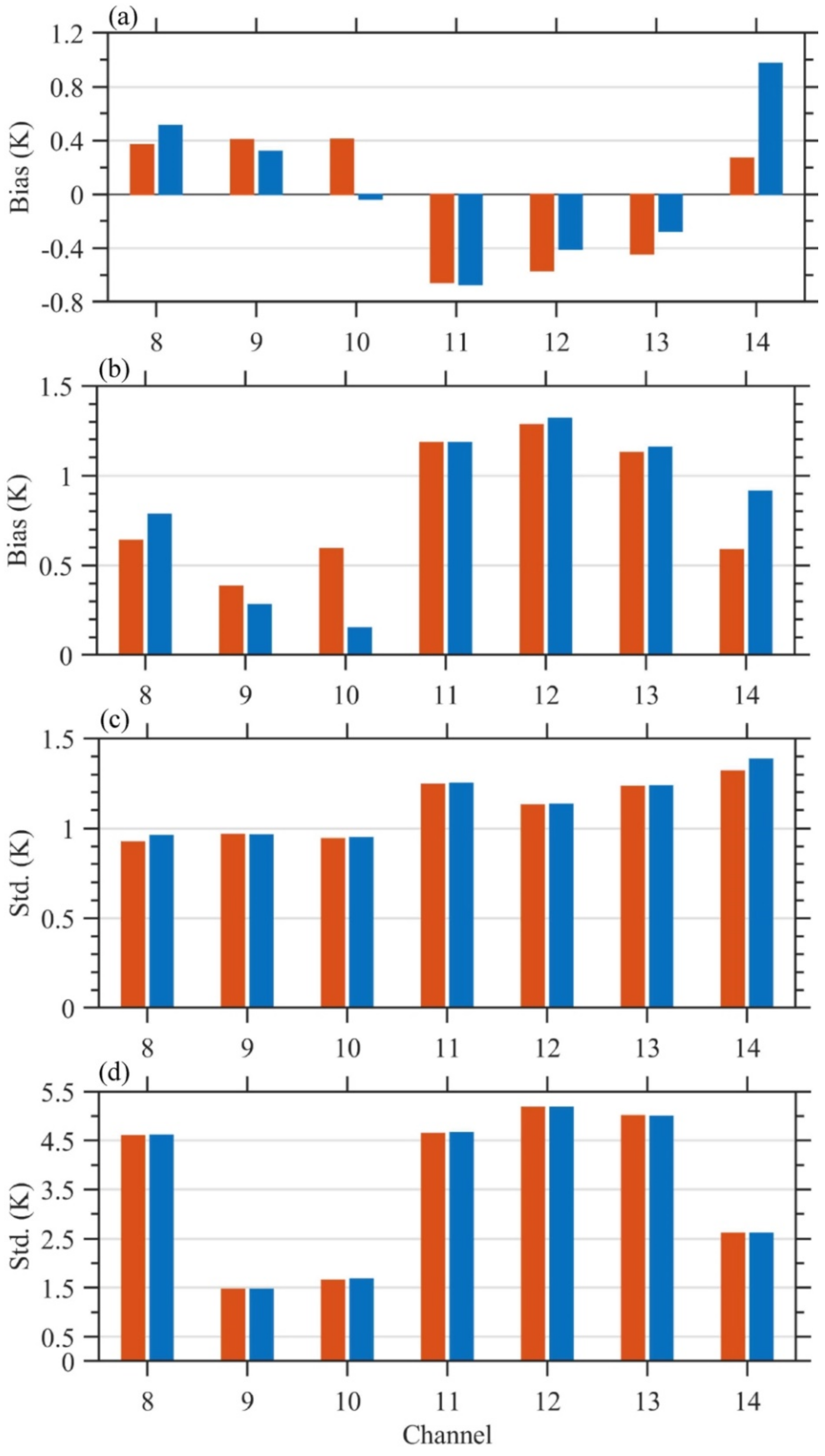
Figure 6 demonstrates that the discrepancies of the OMB results between two models at the AGRI surface–sensitive bands 11–13 were negligible, with a magnitude less than 0.2 K, regardless of whether they were over the ocean or over land. However, large discrepancies were found at band 8 and three gas absorption bands (9, 10, and 14). The OMBARMS of bands 8 and 14 were smaller than those of OMBRTTOV, while the OMBARMS of water vapor bands 9 and 10 were larger than OMBRTTOV. The largest discrepancy was 0.7 K, which occurred at band 14 over the ocean. The differences in the OMB values at non–surface–sensitive bands may be induced in the calculation of absorption coefficients by the two models. There is little difference in the standard deviation of OMBARMS and OMBRTTOV, both over land and the ocean. The results suggest that ARMS has an acceptable capability to simulate IR clear–sky observations.

5. Results

5.1. Spatical Distrubutions of AGRI Biases

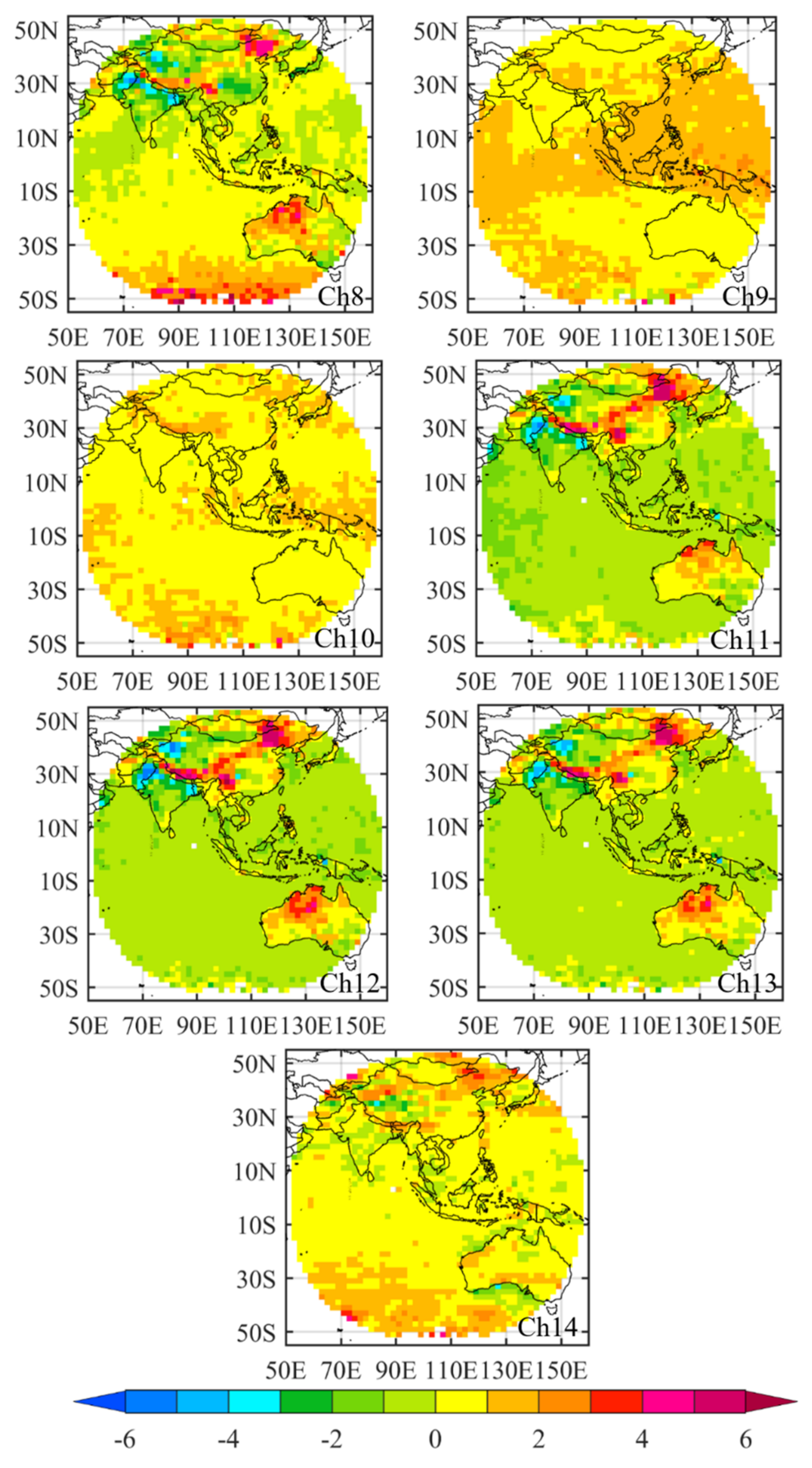
AGRI biases are estimated by the differences between the AGRI observations and ARMS simulations with the FNL dataset as input (OMBFNL). Figure 7 presents the spatial distributions of the mean biases calculated based on OMBFNL for AGRI bands 8–14 within the 2° × 2° grid boxes, respectively. Bands 8, 9, 10, and 14 show systematic positive biases, while bands 11, 12, and 13 show systematic negative biases. The biases over the ocean are relatively homogeneous, with an amplitude of less than 1 K. Over land, spatial distributions of biases are heterogeneous, especially for the surface–sensitive bands. The biases of several degrees in magnitude are positive over Northeastern China, the Tibetan Plateau, as well as Central and Western Australia, with a maximum value reaching 6 K. This is due to the radiance simulations in these areas not being as accurate as those over the ocean.

5.2. Seasonal Variations of Biases at Surface-Sensitive Bands 11–13

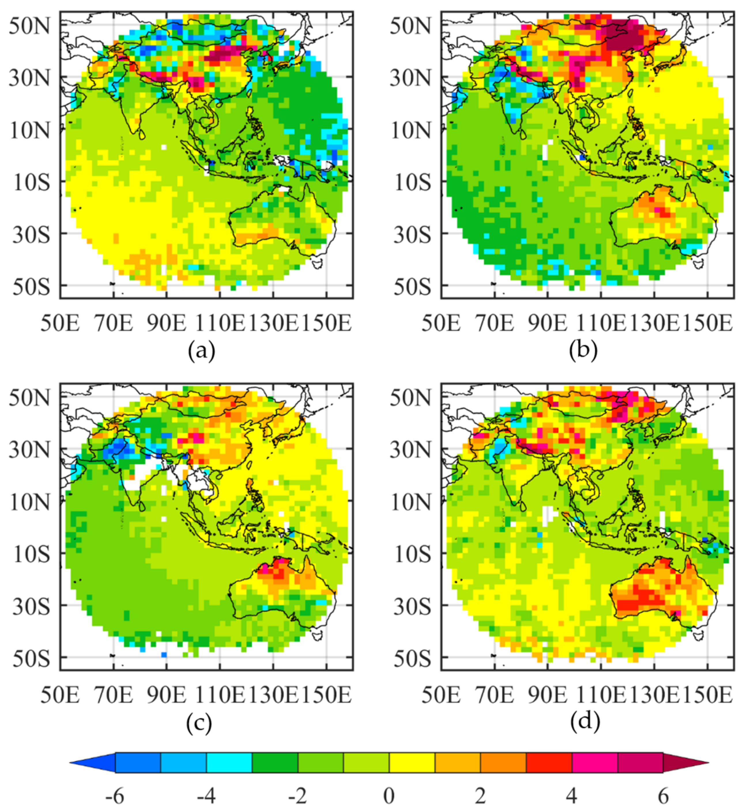
Seasonal variations in the spatial distribution of OMBFNL biases were also investigated. Figure 8 presents the bias distributions in January, April, July, and October 2019, which represents the four seasons of spring, summer, autumn, and winter, respectively, using band 11 as an example (figures for the other bands were omitted). Note that no clear–sky data were found over the Indian Subcontinent and Indo–China Peninsula in July (Figure 8c). This is due to the MOD35 algorithm usually misjudging clear–sky pixels as water-phase clouds during the summer season there, as demonstrated by Zhuge et al. [10].
In April and July (i.e., boreal spring and summer), biases show a negative spatial signature in the southwest (Indian Ocean) and a positive one in the northeast (western North Pacific) over the full disk of AGRI (Figure 8b,c). By contrast, the opposite characteristics were found in the boreal autumn and winter seasons (Figure 8a,d). This transition is caused by the FY–4A satellite’s U–turn at the vernal and autumnal equinoxes every year [51].
Season variations were also found at the two other surface–sensitive bands, i.e., AGRI bands 12 and 13, although the magnitude for bands 12 and 13 was not as significant as it was for band 11. The results again demonstrate the heterogeneous distribution of AGRI observation biases.

5.3. Mean Biases over Ocean and Land

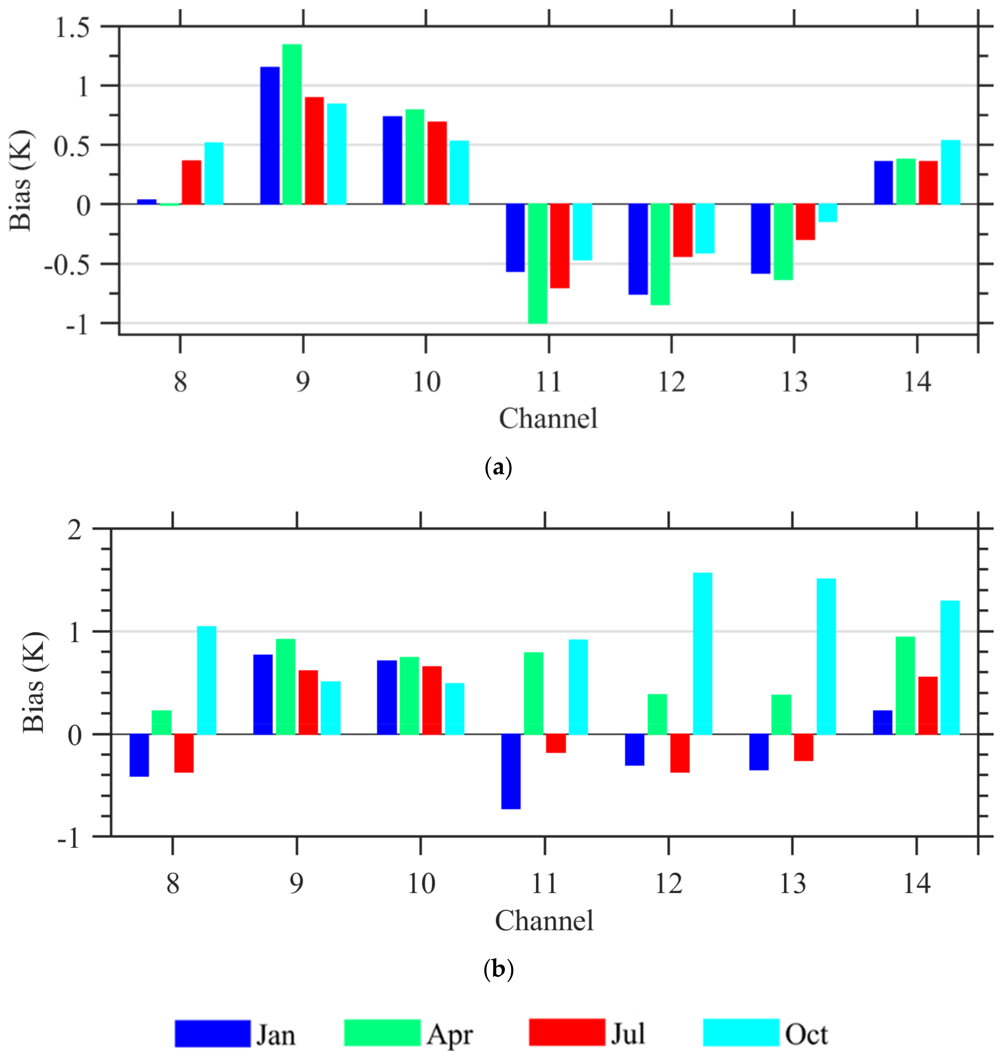
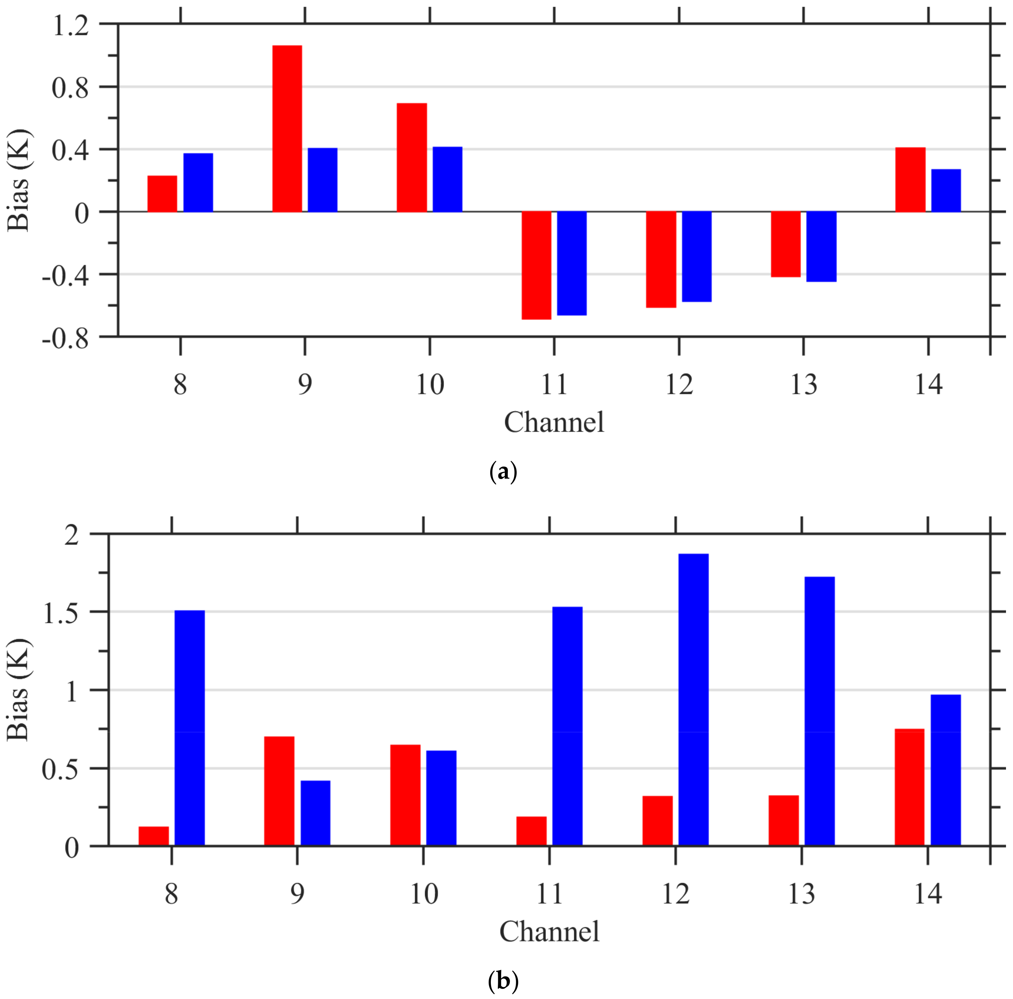
The mean biases of AGRI bands 8–14 in January, April, July, and October 2019, calculated by OMBFNL statistics over the ocean and land, are shown in Figure 9. Any data with a satellite zenith angle greater than 60° were removed because of the large uncertainty in the ARMS simulations. As can be seen in Figure 9, there were significant seasonal differences in the mean biases of surface–sensitive bands 8 and 11–13, and of carbon dioxide absorption band 14 over land. Among them, the biases at bands 8 and 11–13 were negative in January and July, and positive in April and October. This seasonal difference in the biases may be due to the uncertainty in the surface emissivity in the complex land surface region. For biases over the ocean, the seasonal differences in biases were less pronounced than those over land. The biases at band 8 over the ocean in July and October were greater than in January and April, while biases at the other bands were relatively large in April.
Table 3 provides the final biases and standard deviations, spatially and temporally averaged over the ocean and land over four months. Overall, OMBFNL biases for all seven IR bands of AGRI were within −0.7 to 1.1 K for infrared bands over the ocean under clear-sky conditions, while 0.12~0.75 K was found over land. The standard deviations for OMBFNL statistics over land were greater than over the ocean, suggesting larger uncertainties in simulations over land than those over the ocean.

5.4. Bias Dependences on Satellite Zenith Angle

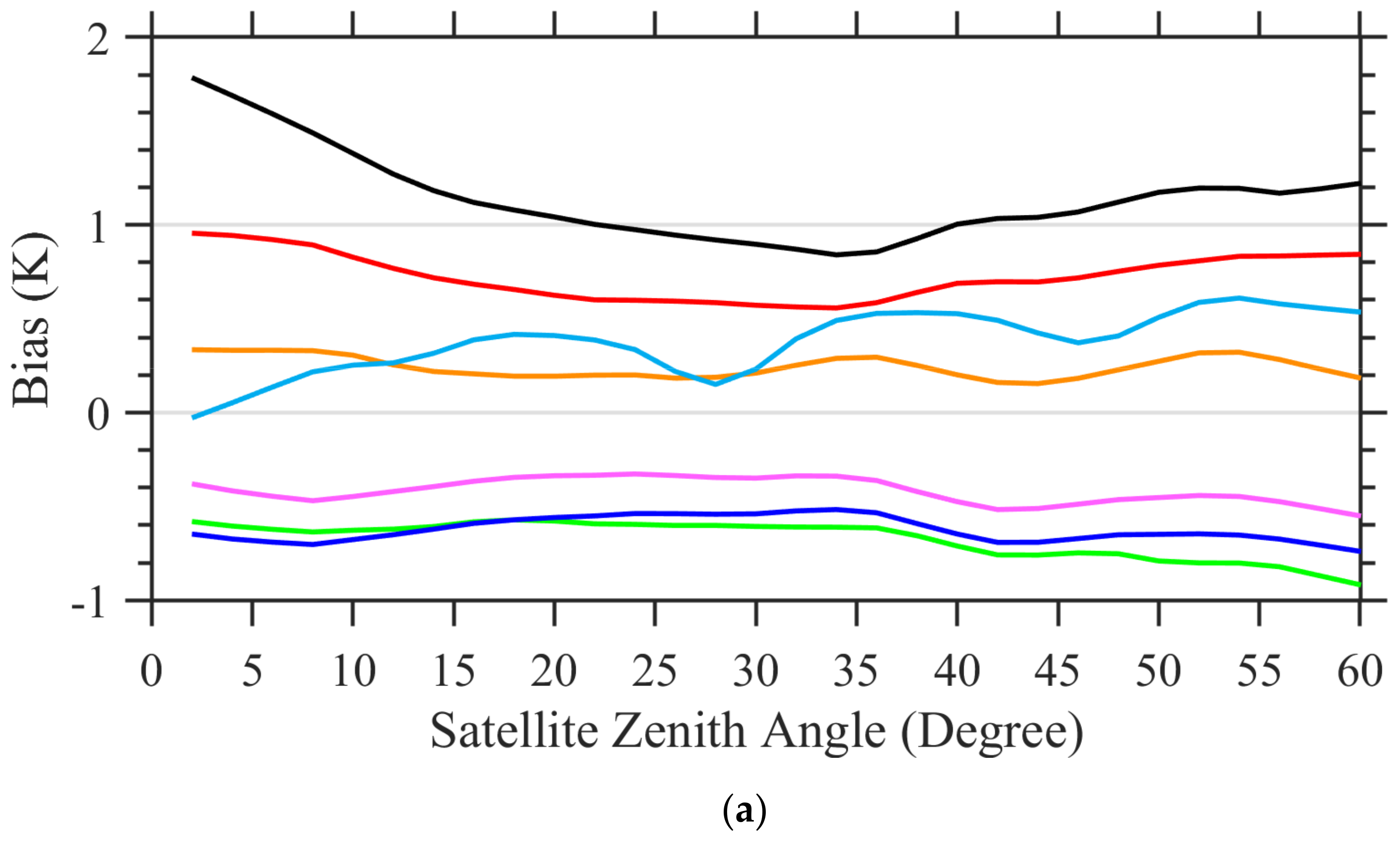
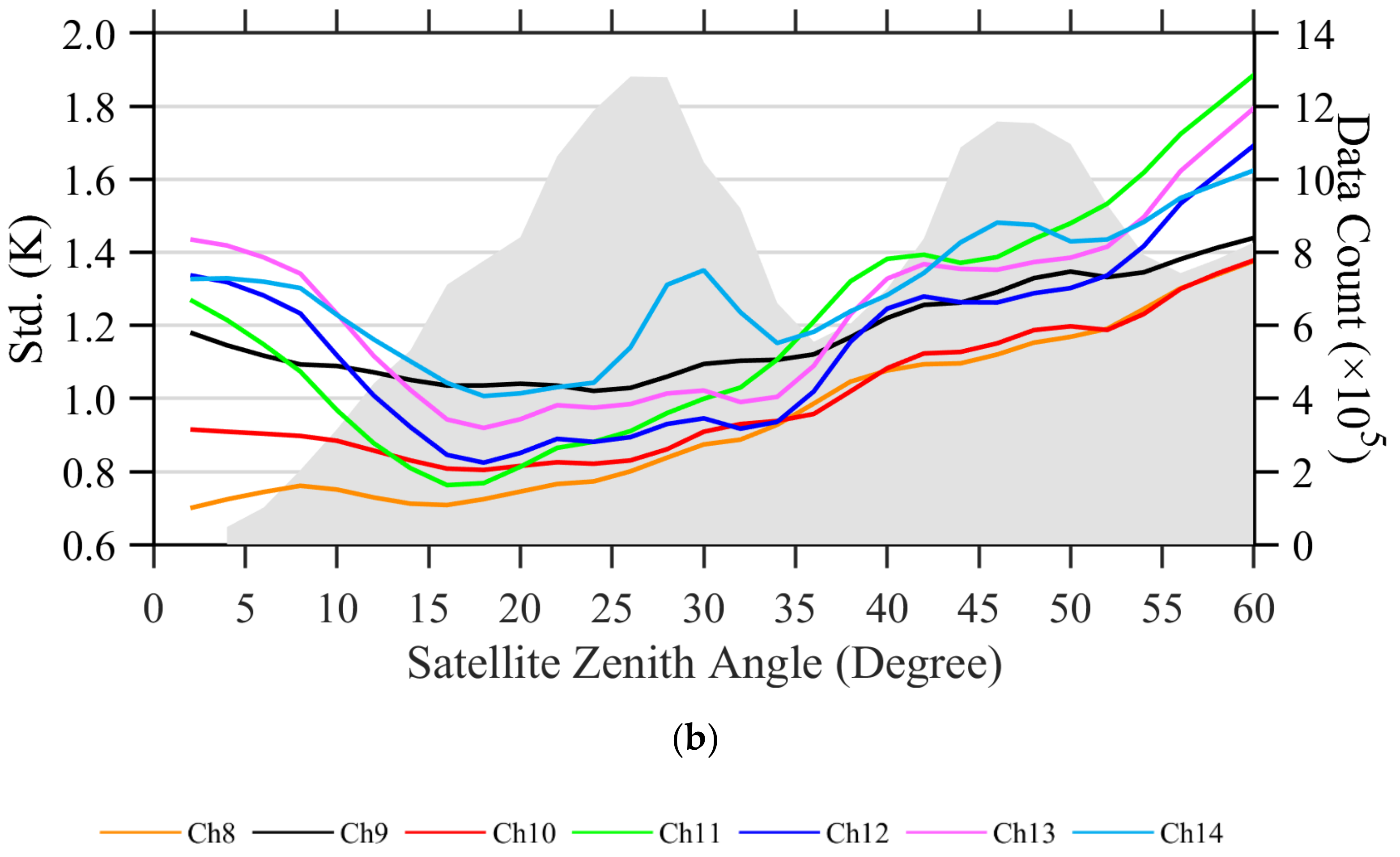
For the majority of cross–track scanning instruments onboard polar–orbiting satellites, a scan–angle (or satellite-zenith-angle) dependent bias was typically observed. Since the optical path increased with the satellite zenith angle, the uncertainties in the model simulations likely increased. For a geostationary satellite imager like AGRI, it was also necessary to examine the OMBFNL versus the satellite zenith angle. Variations in the biases and standard deviations of OMBFNL differences with respect to satellite zenith angle are presented in Figure 10. Note that data over land are not included because of the uncertainties in land simulations. It can be seen from Figure 10a that there is no obvious dependence on the satellite zenith angle for OMBFNL biases in bands 8 and 11–13, while in bands 9, 10, and 14, the OMBFNL shows a strong dependence on the satellite zenith angle. The standard deviations of IR bands 8–14 vary with data counts and satellite zenith angle (Figure 10b).

5.5. Bias Dependences on Scene Temperature

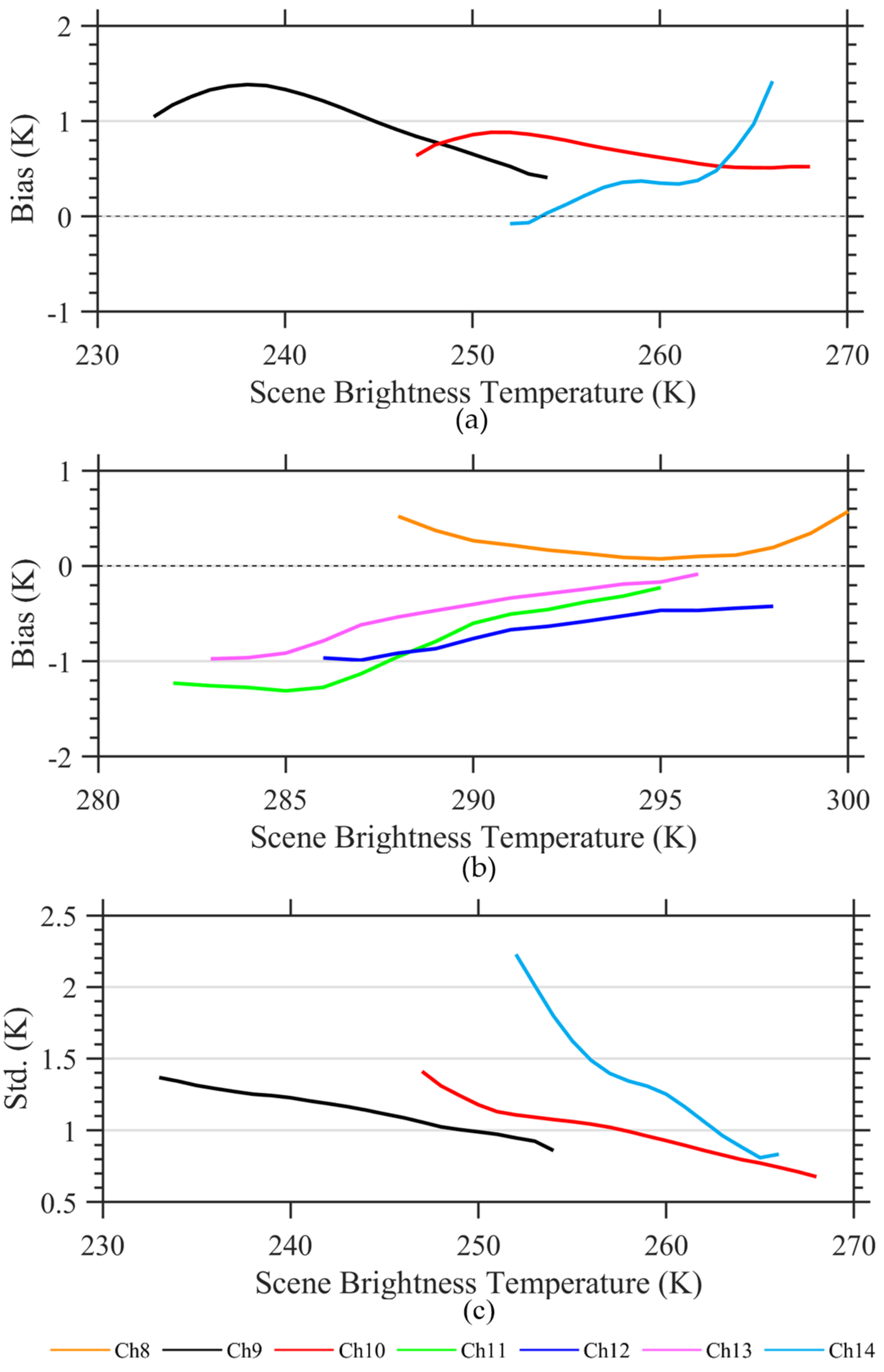
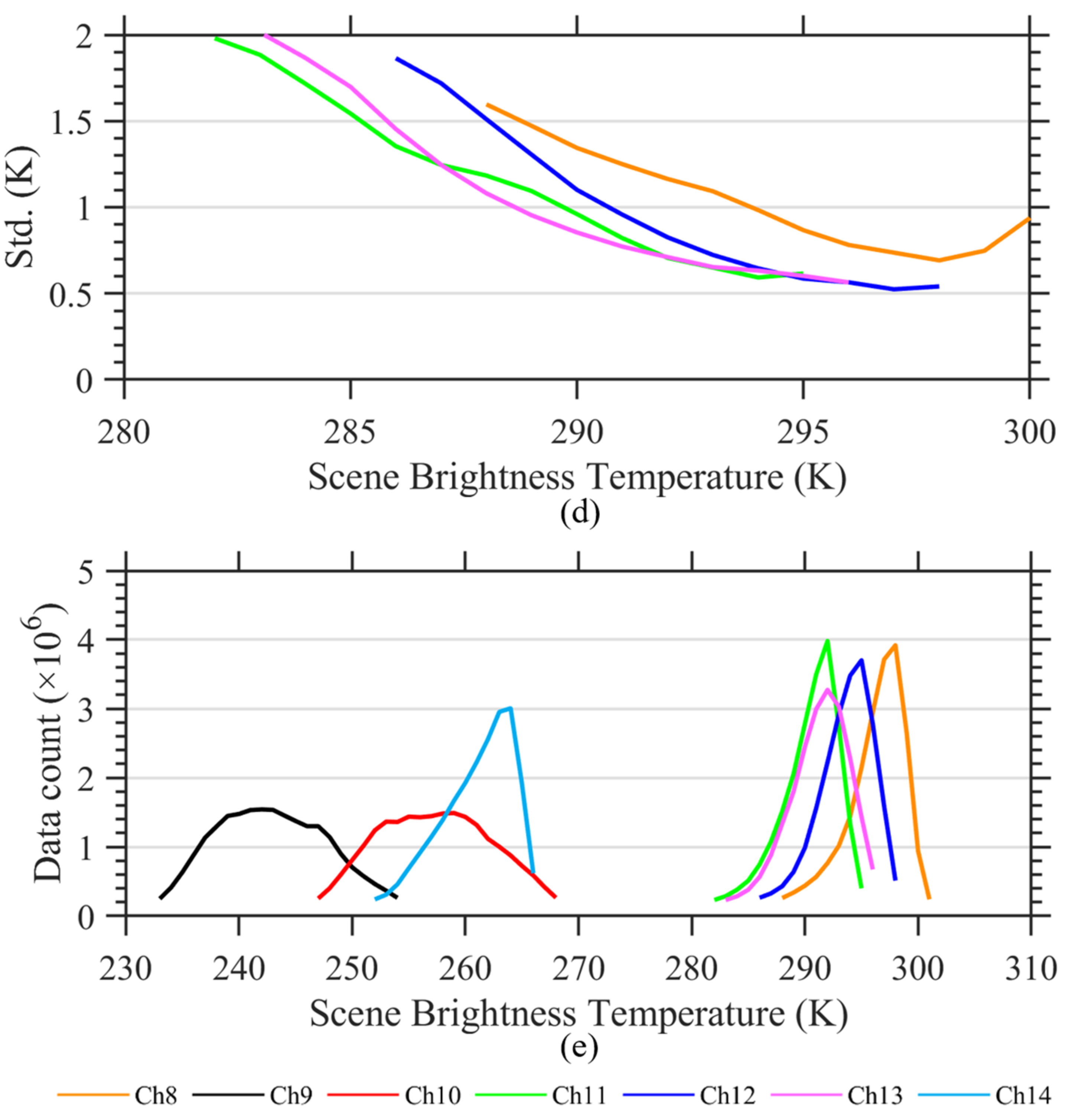
The dependence of OMBFNL biases on scene brightness temperatures with a satellite zenith angle less than 60° is examined here. Figure 11 shows variations in the biases and standard deviations of OMBFNL, as well as data counts with respect to scene brightness temperatures.
As shown in Figure 11a,b, an obvious scene–temperature dependence of the OMB biases for AGRI bands 8–14 exists. For surface–sensitive bands 11, 12, and 13, and carbon dioxide absorption band 14, the OMB biases increased by almost 1 K with an increasing brightness temperature. The OMB biases for band 8 decreased first and then increased with the brightness temperature, reaching a minimum at 295 K. For the two water vapor bands 9 and 10, the OMBFNL biases first increased to a maximum and then decreased as the brightness temperature increased. The standard deviations of bands 8–14 decreased with an increasing brightness temperature (Figure 11c,d).
The AGRI is a radiometric calibration that uses a built–in blackbody as a hot target and a cold–sky as a cold target. This calibration is based on the assumption of a linear response of the instrument to incident radiation, which is nonlinear in practice. Zou et al. [23] suggested that the nonlinear nature of the instrument is the main reason for the dependence of bias on brightness temperature.

6. Difference of Mean Biases Based on FNL and ERA5

The biases of OMBFNL for bands 8–14 were compared with those calculated by ARMS with the ERA5 dataset as the input (OMBERA5), and differences were found between OMBFNL and OMBERA5 at some bands. From Figure 12, it is clear that there are obvious differences (almost 1.5 K) between OMBFNL and OMBERA5 for surface–sensitive bands 8 and 11–13 over land, and the OMBERA5 biases were greater than the OMBFNL biases. Over the ocean, the OMBFNL was only greater than OMBERA5 at water vapor absorption bands 9 and 10, while other bands did not differ much from each other. The reasons for the differences between OMBFNL and OMBERA5 are given in the following subsection.

6.1. Skin Temperature Difference between FNL and ERA5 Datasets

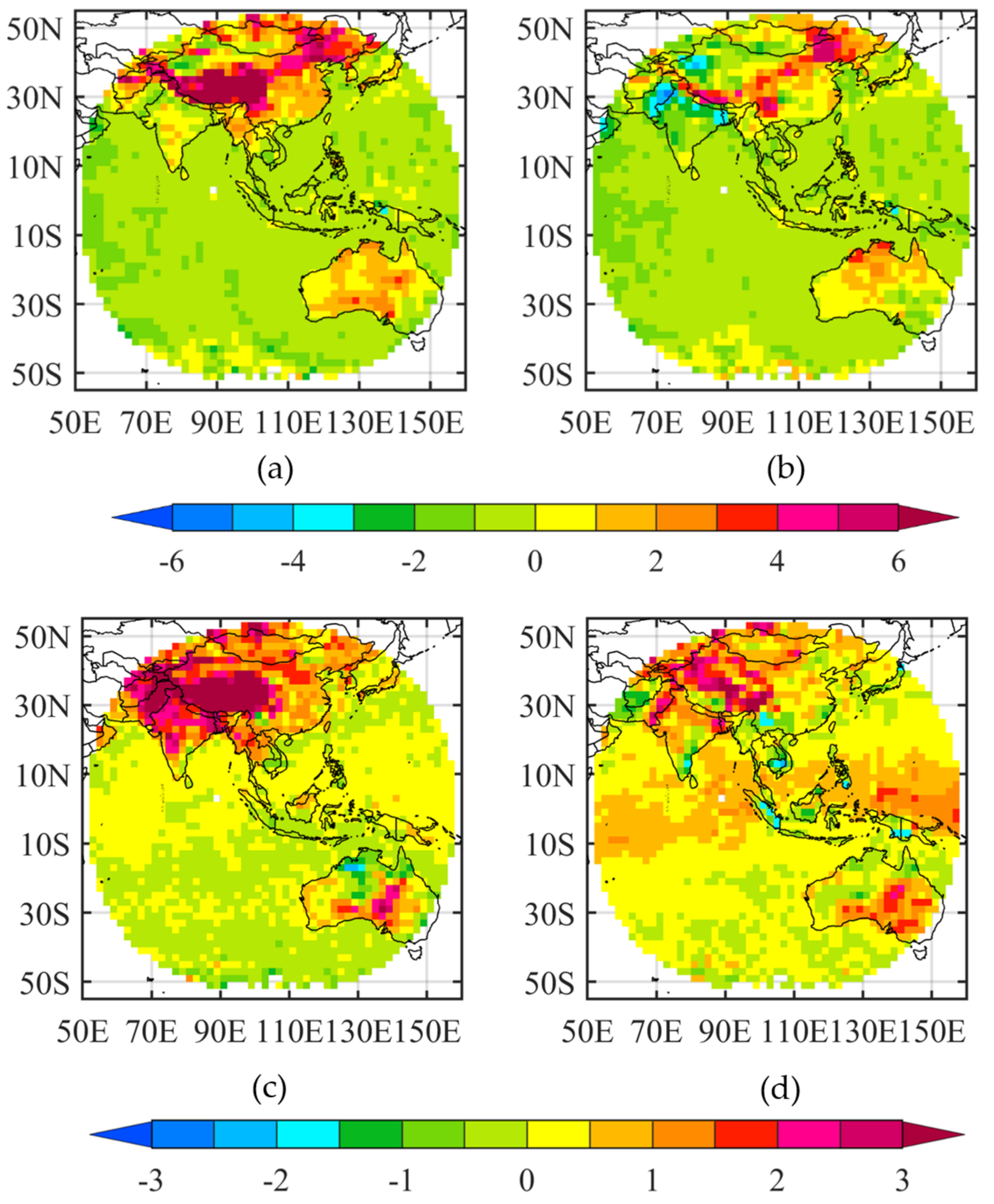
Both the OMBERA5 and OMBFNL biases are significantly greater over land than over the oceans, as shown in Figure 13a,b for AGRI band 11 (similar results were found for bands 12 and 13; figures omitted). Trigo et al. [52] pointed out that the land skin temperatures in ECMWF analyses and forecasts had, on average, a cold bias (a warm bias during the nighttime and a large, cold bias during the daytime) over arid and semiarid regions. As a result, the simulated radiance was in general lower than the observed one over these regions. Moreover, over the Tibetan Plateau and Central Australia, the amplitude of bias calculated from OMBERA5 was larger than that from OMBFNL (Figure 13c).
A spatial distribution of skin temperature differences between FNL and ERA5 (FNL minus ERA5) is given in Figure 13d. It shows positive values over the Tibetan Plateau and Central Australia, which correspond to the areas with significant discrepancies between OMBERA5 and OMBFNL in Figure 13c. Over the ocean, the differences in skin temperature in the FNL and ERA5 datasets were small everywhere; thus, the differences between OMBFNL and OMBERA5 were small.

6.2. Atmospheric Profiles Differences between FNL and ERA5 Datasets

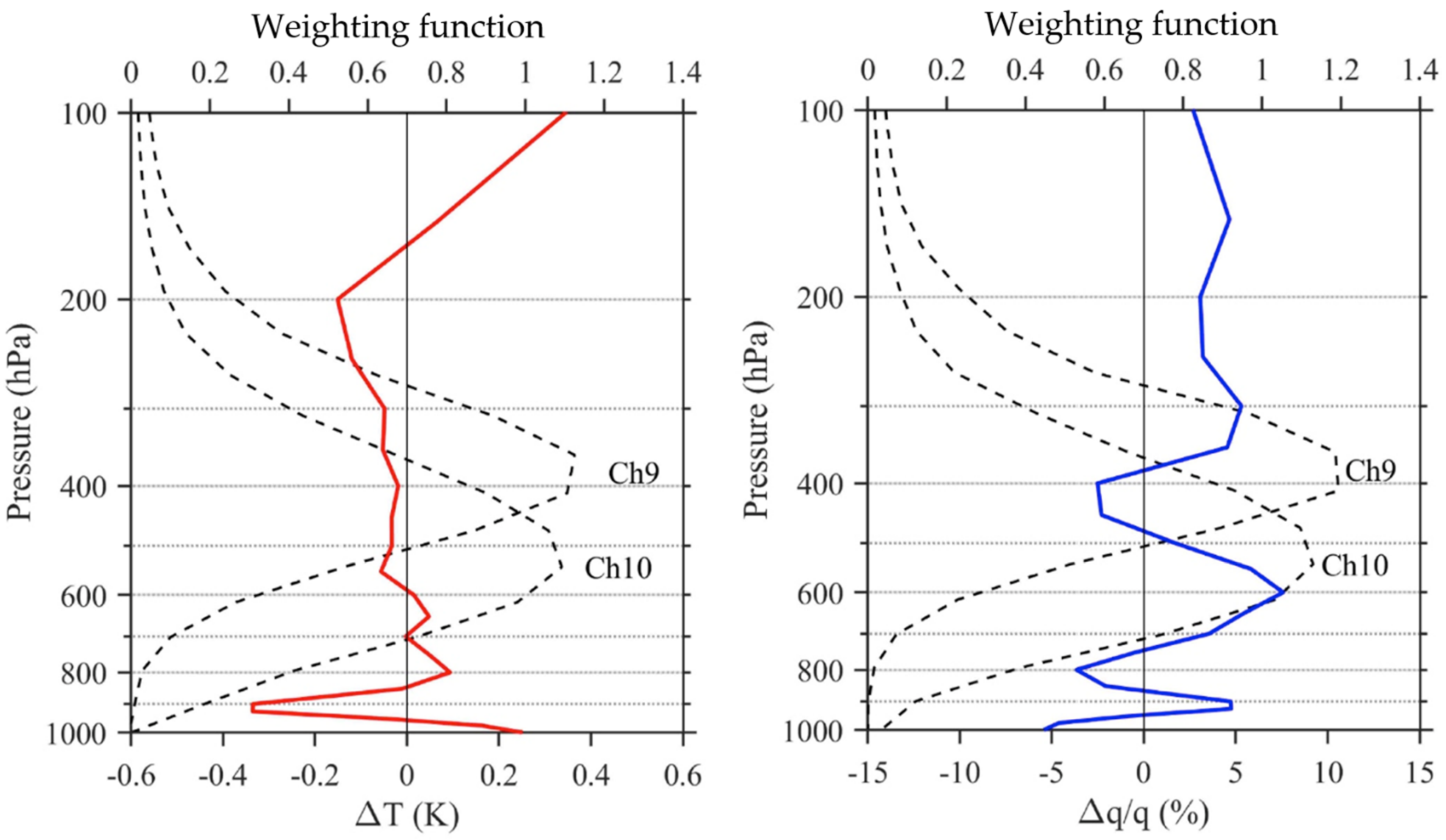
The differences between the OMBFNL and OMBERA5 at two water vapor bands, 9 and 10, were attributed to the differences in the humidity and temperature profiles between the ERA5 and FNL datasets. As seen in Figure 14, the average FNL data at 0000, 0600, 1200, and 1800 UTC was wetter at 300 hPa and 600 hPa, but drier at 450 hPa and colder above the 600 hPa pressure level than the ERA5 data. By overlapping the vertical distributions of differences between ERA5 and FNL onto the weighting functions of the two water vapor bands in Figure 14, it is clear that a deep, wetter layer extending from 250 to nearly 400 hPa was right above the weighting function peak level of AGRI band 9. As a result, the simulated radiance decreased due to absorption and re–emission from the upper–tropospheric water vapor. Meanwhile, a colder layer from 200 to 600 hPa coincided with the weighting function peak levels of two water vapor bands. Since the temperature at the weighting function peak level contributed the most to the simulated radiance, a mid–troposphere colder layer resulted in small simulated radiances. The weighting functions were calculated using the US 1976 standard atmosphere. Note that the location of a peak of a weighting function actually varies in time due to variations in the vertical structure of both temperature and water vapor in clear–sky scenes. However, the two factors mentioned above indeed contributed to the large, positive values of OMBFNL statistics.

7. Conclusions

The newly developed ARMS model was employed to characterize biases of AGRI’s seven 4 km–resolution IR bands. The FNL dataset was utilized as input for ARMS. By a quality control, AGRI data around mid–night before and after the vernal and autumnal equinoxes were removed due to brightness temperature anomalies at band 8 caused by the stray light contamination. Besides, considering the highest accuracy of model simulations of radiance under clear–sky conditions, the cloud–contaminated data were removed by collocating MOD35 cloud mask products with AGRI pixels.
The spatial distributions of AGRI biases were homogeneous over the ocean, with mean biases less than 1 K at all IR bands. Over land, biases for surface–sensitive bands were heterogeneously distributed; characterized by positive biases over Northeastern China, the Tibetan Plateau, as well as Central and Western Australia; and the maximum value of the biases over these regions reached 6 K. The seasonal characteristics of AGRI bands 8–14 bias were analyzed using data from January, April, July, and October 2019, and bands 11–13 showed seasonal variations in spatial distributions. Bands 8–14 showed biases that were dependent on the satellite zenith angle and scene temperature. The uncertainties in the NWP background data of land skin temperature were the main cause of the heterogeneous distributions of AGRI biases.
The AGRI total mean biases of bands 8–14 were smaller than 1.1 K in magnitude when using either the FNL or ERA5 dataset over the ocean. The biases of water vapor bands were much larger when using FNL due to a wet bias in the upper troposphere and a cold bias in the middle troposphere of the FNL data.

Author Contributions

Conceptualization, F.T. and X.Z.; methodology, F.T. and X.Z.; software, F.T., P.D. and Y.H.; validation, F.T., X.Z., M.Z., P.D., Y.H. and X.L.; formal analysis, F.T.; investigation, F.T.; resources, F.T. and M.Z.; data curation, F.T., X.Z. and X.L.; writing—original draft preparation, F.T.; writing—review and editing, F.T., X.Z. and X.L. All authors have read and agreed to the published version of the manuscript.

Funding

This research was supported by the National Key R&D Program of China (Grant 2017YFC1501805), the Natural Science Foundation of Jiangsu Province (Grant BK20201505), the Youth Fund Project of Jiangsu Meteorological Bureau (Grant KQ202007), the Basic Research Found of Chinese Academy of Meteorological Sciences (2021Z002, 2020R002, 2021Y013, and 2021Y014), the Open Grants of State Key Laboratory of Severe Weather (2020LASW-B11), and the National Science Foundation of China (41805076).

Institutional Review Board Statement

Not applicable.

Informed Consent Statement

Not applicable.

Data Availability Statement

Not applicable.

Acknowledgments

The authors would like to thank Fuzhong Weng for his valuable suggestions and support during study. Wanlin Kan is thanked for her suggestions on brightness temperature simulation of AGRI IR bands. We thank the NSMC of the CMA for providing FY-4A/AGRI data (http://satellite.nsmc.org.cn/PortalSite/Data/Satellite.aspx?currentculture=en-US, accessed on 25 February 2020), the ECMWF for providing ERA5 (https://cds.climate.copernicus.eu/#!/search?text=ERA5&type=dataset, accessed on 1 January 2020), the NCAR for providing NCEP_FNL data (https://rda.ucar.edu/, accessed on 20 December 2020), and NASA for proving MOD35 data (https://ladsweb.modaps.eosdis.nasa.gov, accessed on 19 August 2020).

Conflicts of Interest

The authors declare no conflict of interest.

References

  1. Bessho, K.; Date, K.; Hayashi, M.; Ikeda, A.; Imai, T.; Inoue, H.; Kumagai, Y.; Miyakawa, T.; Murata, H.; Ohno, T.; et al. An Introduction to Himawari-8/9—Japan’s New-Generation Geostationary Meteorological Satellites. J. Meteorol. Soc. Jpn. 2016, 94, 151–183. [Google Scholar] [CrossRef] [Green Version]
  2. Schmit, T.J.; Lindstrom, S.S.; Gerth, J.J.; Gunshor, M.M. Applications of the 16 spectral bands on the Advanced Baseline Imager (ABI). J. Oper. Meteorol. 2018, 6, 33–46. [Google Scholar] [CrossRef]
  3. Zou, X.; Qin, Z.; Weng, F. Improved coastal precipitation forecast with direct assimilation of GOES 11/12 imager radiances. Mon. Weather Rev. 2011, 139, 3711–3729. [Google Scholar] [CrossRef] [Green Version]
  4. Zou, X.; Qin, Z.; Zheng, Y. Improved Tropical Storm Forecasts with GOES-13/15 Imager Radiance Assimilation and Asymmetric Vortex Initialization in HWRF. Mon. Weather Rev. 2015, 143, 2485–2505. [Google Scholar] [CrossRef]
  5. Ma, Z.; Maddy, E.S.; Zhang, B.; Zhu, T.; Boukabara, S.A. Impact Assessment of Himawari-8 AHI Data Assimilation in NCEP GDAS/GFS with GSI. J. Atmos. Ocean. Technol. 2017, 34, 797–815. [Google Scholar] [CrossRef]
  6. Wang, P.; Li, J.; Lu, B.; Schmit, T.J.; Lu, J.; Lee, Y.-K.; Li, J.; Liu, Z. Impact of Moisture Information From Advanced Himawari Imager Measurements on Heavy Precipitation Forecasts in a Regional NWP Model. J. Geophys. Res. Atmos. 2018, 123, 6022–6038. [Google Scholar] [CrossRef]
  7. Wang, Y.; Liu, Z.; Yang, S.; Min, J.; Chen, L.; Chen, Y.; Zhang, T. Added Value of Assimilating Himawari-8 AHI Water Vapor Radiances on Analyses and Forecasts for “7.19” Severe Storm Over North China. J. Geophys. Res. Atmos. 2018, 123, 3374–3394. [Google Scholar] [CrossRef]
  8. Zhuge, X.; Zou, X. Summertime Convective Initiation Nowcasting over Southeastern China Based on Advanced Himawari Imager Observations. J. Meteorol. Soc. Jpn. Ser. II 2018, 96, 337–353. [Google Scholar] [CrossRef] [Green Version]
  9. Min, M.; Bai, C.; Guo, J.; Sun, F.; Liu, C.; Wang, F.; Xu, H.; Tang, S.; Li, B.; Di, D.; et al. Estimating Summertime Precipitation from Himawari-8 and Global Forecast System Based on Machine Learning. IEEE Trans. Geosci. Remote Sens. 2018, 57, 2557–2570. [Google Scholar] [CrossRef]
  10. Zhuge, X.; Zou, X.; Wang, Y. Determining AHI Cloud-Top Phase and Intercomparisons With MODIS Products Over North Pacific. IEEE Trans. Geosci. Remote. Sens. 2021, 59, 1–13. [Google Scholar] [CrossRef]
  11. Min, M.; Li, J.; Wang, F.; Liu, Z.; Menzel, W.P. Retrieval of cloud top properties from advanced geostationary satellite imager measurements based on machine learning algorithms. Remote Sens. Environ. 2020, 239, 111616. [Google Scholar] [CrossRef]
  12. Li, R.; Li, H.; Sun, L.; Yang, Y.; Hu, T.; Bian, Z.; Cao, B.; Du, Y.; Liu, Q. An Operational Split-Window Algorithm for Retrieving Land Surface Temperature from Geostationary Satellite Data: A Case Study on Himawari-8 AHI Data. Remote Sens. 2020, 12, 2613. [Google Scholar] [CrossRef]
  13. Gültepe, I.; Pagowski, M.; Reid, J. A Satellite-Based Fog Detection Scheme Using Screen Air Temperature. Weather Forecast 2007, 22, 444–456. [Google Scholar] [CrossRef]
  14. Gunshor, M.M.; Schmit, T.J.; Menzel, W.P. Intercalibration of the infrared window and water vapor bands on operational geostationary environmental satellites using a single polar-orbiting satellite. J. Atmos. Oceanic Technol. 2004, 21, 61–68. [Google Scholar] [CrossRef]
  15. Yu, F.; Wu, X. Radiometric Inter-Calibration between Himawari-8 AHI and S-NPP VIIRS for the Solar Reflective Bands. Remote Sens. 2016, 8, 165. [Google Scholar] [CrossRef] [Green Version]
  16. Li, X.; Zou, X. Bias characterization of CrIS radiances at 399 selected channels with respect to NWP model simulations. Atmos. Res. 2017, 196, 164–181. [Google Scholar] [CrossRef]
  17. Kalnay, E. Atmospheric Modeling, Data Assimilation and Predictability; Cambridge University Press: Cambridge, UK, 2003. [Google Scholar]
  18. Weng, F.; Zou, X.; Wang, X.; Yang, S.; Goldberg, M.D. Introduction to Suomi national polar-orbiting partnership advanced technology microwave sounder for numerical weather prediction and tropical cyclone applications. J. Geophys. Res. Space Phys. 2012, 117, 117. [Google Scholar] [CrossRef]
  19. Saunders, R.; Matricardi, M.; Brunel, P. An improved fast radiative transfer model for assimilation of satellite radiance observations. Q. J. R. Meteorol. Soc. 1999, 125, 1407–1425. [Google Scholar] [CrossRef]
  20. Matricardi, M.; Chevallier, F.; Kelly, G.; Thépaut, J.-N. An improved general fast radiative transfer model for the assimilation of radiance observations. Q. J. R. Meteorol. Soc. 2004, 130, 153–173. [Google Scholar] [CrossRef]
  21. Weng, F. Advances in Radiative Transfer Modeling in Support of Satellite Data Assimilation. J. Atmos. Sci. 2007, 64, 3799–3807. [Google Scholar] [CrossRef]
  22. Han, Y.; Weng, F.; Liu, Q.; Van Delst, P. A fast radiative transfer model for SSMIS upper atmosphere sounding channels. J. Geophys. Res. Space Phys. 2007, 112. [Google Scholar] [CrossRef]
  23. Zou, X.; Zhuge, X.; Weng, F. Characterization of bias of Advanced Himawari Imager infrared observations from NWP back-ground simulations using CRTM and RTTOV. J. Atmos. Oceanic Technol. 2016, 33, 2553–2567. [Google Scholar] [CrossRef]
  24. Li, X.; Zou, X.; Zhuge, X.; Zeng, M.; Wang, N.; Tang, F. Improved Himawari-8/AHI Radiance Data Assimilation With a Double Cloud Detection Scheme. J. Geophys. Res. Atmos. 2020, 125. [Google Scholar] [CrossRef]
  25. Honda, T.; Miyoshi, T.; Lien, G.-Y.; Nishizawa, S.; Yoshida, R.; Adachi, S.; Terasaki, K.; Okamoto, K.; Tomita, H.; Bessho, K. Assimilating All-Sky Himawari-8 Satellite Infrared Radiances: A Case of Typhoon Soudelor (2015). Mon. Weather Rev. 2018, 146, 213–229. [Google Scholar] [CrossRef]
  26. Qin, Z.; Zou, X.; Weng, F. Impacts of assimilating all or GOES-like AHI infrared channels radiances on QPFs over Eastern China. Tellus A Dyn. Meteorol. Oceanogr. 2017, 69, 1345265. [Google Scholar] [CrossRef]
  27. Qu, J.H.; Zhang, L.; Lu, Q.F.; Zhang, N.Q.; Wang, D. Characterization of bias in FY-4A advanced geostationary radiation imager observations from ERA5 background simulations using RTTOV. Acta. Meteorol. Sinica. 2019, 77, 911–922. Available online: http://html.rhhz.net/qxxb_cn/html/2019049.htm (accessed on 14 May 2017).
  28. Geng, X.; Min, J.Z.; Yang, C.; Wang, B.; Xu, D. Analysis of FY-4A AGRI radiance data bias characteristics and a correction experiment. Chin. J. Atmos. Sci. 2020, 44, 679–694. [Google Scholar] [CrossRef]
  29. Zhu, J.; Shu, J.; Guo, W. Biases Characteristics Assessment of the Advanced Geosynchronous Radiation Imager (AGRI) Measurement on Board Fengyun–4A Geostationary Satellite. Remote Sens. 2020, 12, 2871. [Google Scholar] [CrossRef]
  30. Weng, F.; Yu, X.; Duan, Y.; Yang, J.; Wang, J. Advanced Radiative Transfer Modeling System (ARMS): A New-Generation Satellite Observation Operator Developed for Numerical Weather Prediction and Remote Sensing Applications. Adv. Atmos. Sci. 2020, 37, 131–136. [Google Scholar] [CrossRef] [Green Version]
  31. Yang, J.; Ding, S.; Dong, P.; Bi, L.; Yi, B. Advanced radiative transfer modeling system developed for satellite data assimilation and remote sensing applications. J. Quant. Spectrosc. Radiat. Transf. 2020, 251, 107043. [Google Scholar] [CrossRef]
  32. Liu, Q.; Weng, F. A Microwave Polarimetric Two-Stream Radiative Transfer Model. J. Atmos. Sci. 2002, 59, 2396–2402. [Google Scholar] [CrossRef]
  33. Shi, Y.-N.; Yang, J.; Weng, F. Discrete Ordinate Adding Method (DOAM), a new solver for Advanced Radiative transfer Modeling System (ARMS). Opt. Express 2021, 29, 4700–4720. [Google Scholar] [CrossRef] [PubMed]
  34. Liu, Q.; Weng, F. Advanced Doubling–Adding Method for Radiative Transfer in Planetary Atmospheres. J. Atmos. Sci. 2006, 63, 3459–3465. [Google Scholar] [CrossRef]
  35. Evans, K.; Stephens, G. A new polarized atmospheric radiative transfer model. J. Quant. Spectrosc. Radiat. Transf. 1991, 46, 413–423. [Google Scholar] [CrossRef]
  36. Weng, F. A multi-layer discrete-ordinate method for vector radiative transfer in a vertically-inhomogeneous, emitting and scattering atmosphere—I. Theory. J. Quant. Spectrosc. Radiat. Transf. 1992, 47, 19–33. [Google Scholar] [CrossRef]
  37. Weng, F. Passive Microwave Remote Sensing of the Earth: For Meteorological Applications; Wiley: Hoboken, NJ, USA, 2017; p. 384. [Google Scholar]
  38. Schulz, F.; Stamnes, K.; Weng, F. Vdisort: An improved and generalized discrete ordinate method for polarized (vector) radiative transfer. J. Quant. Spectrosc. Radiat. Transf. 1999, 61, 105–122. [Google Scholar] [CrossRef]
  39. Kummerow, C. On the accuracy of the Eddington approximation for radiative transfer in the microwave frequencies. J. Geophys. Res. Space Phys. 1993, 98, 2757–2765. [Google Scholar] [CrossRef]
  40. McMillin, L.M.; Crone, L.J.; Kleespies, T.J. Atmospheric transmittance of an absorbing gas 5 Improvements to the optran approach. Appl. Opt. 1995, 34, 8396–8399. [Google Scholar] [CrossRef]
  41. Gordon, I.E.; Rothman, L.S.; Hill, C.; Kochanov, R.V.; Tan, Y.; Bernath, P.F.; Birk, M.; Boudon, V.; Campargue, A.; Chance, K.V.; et al. The HITRAN2016 molecular spectroscopic database. J. Quant. Spectrosc. Radiat. Transf. 2017, 203, 3–69. [Google Scholar] [CrossRef]
  42. Clough, S.A.; Iacono, M.; Moncet, J.-L. Line-by-line calculations of atmospheric fluxes and cooling rates: Application to water vapor. J. Geophys. Res. Space Phys. 1992, 97, 15761–15785. [Google Scholar] [CrossRef]
  43. Clough, S.; Shephard, M.; Mlawer, E.; Delamere, J.; Iacono, M.; Cady-Pereira, K.; Boukabara, S.A.; Brown, P. Atmospheric radiative transfer modeling: A summary of the AER codes. J. Quant. Spectrosc. Radiat. Transf. 2005, 91, 233–244. [Google Scholar] [CrossRef]
  44. Yang, J.; Zhang, Z.; Wei, C.; Lu, F.; Guo, Q. Introducing the New Generation of Chinese Geostationary Weather Satellites, Fengyun-4. Bull. Am. Meteorol. Soc. 2017, 98, 1637–1658. [Google Scholar] [CrossRef]
  45. Guo, Q.; Xu, J.; Zhang, W. Stray light modelling and analysis for the FY-2 meteorological satellite. Int. J. Remote Sens. 2005, 26, 2817–2830. [Google Scholar] [CrossRef]
  46. Wu, X.; Smith, W.L. Emissivity of rough sea surface for 8–13 µm: Modeling and verification. Appl. Opt. 1997, 36, 2609–2619. [Google Scholar] [CrossRef] [PubMed]
  47. Zhuge, X.; Zou, X.; Weng, F.; Sun, M. Dependence of Simulation Biases at AHI Surface-Sensitive Channels on Land Surface Emissivity over China. J. Atmos. Ocean. Technol. 2018, 35, 1283–1298. [Google Scholar] [CrossRef]
  48. Borbas, E.; Hulley, G.; Knuteson, R.; Feltz, M. MEaSUREs Unified and Coherent Land Surface Temperature and Emissivity (LST&E) Earth System Data Record (ESDR): The Combined ASTER and MODIS Emissivity Database Over Land (CAMEL). 2017. Available online: ftp://ftp.ssec.wisc.edu/pub/ICI/MEASURES_doc/V001/MEaSUREs_CAMEL_Users_Guid323e_02172017.pdf (accessed on 17 February 2017).
  49. Wang, X.; Min, M.; Wang, F.; Guo, J.; Li, B.; Tang, S. Intercomparisons of Cloud Mask Products Among Fengyun-4A, Himawari-8, and MODIS. IEEE Trans. Geosci. Remote Sens. 2019, 57, 8827–8839. [Google Scholar] [CrossRef]
  50. Ackerman, S.; Strabala, K.; Menzel, P.; Frey, R.; Moeller, C.; Gumley, L. Discriminating Clear-Sky from Cloud with MODIS; Algorithm Theoretical Basis Document (MOD35) Version 6.1; Wisconsin-Madison University: Madison, WI, USA, 2010. [Google Scholar]
  51. Liu, Y.; Wang, H.; Li, Z.; Wang, Z. A verification of the lightning detection data from FY-4A LMI as compared with ADTD-2. Atmos. Res. 2021, 248, 105163. [Google Scholar] [CrossRef]
  52. Trigo, I.F.; Boussetta, S.; Viterbo, P.; Balsamo, G.; Beljaars, A.; Sandu, I. Comparison of model land skin temperature with remotely sensed estimates and assessment of surface-atmosphere coupling. J. Geophys. Res. Atmos. 2015, 120, 12096–12111. [Google Scholar] [CrossRef] [Green Version]
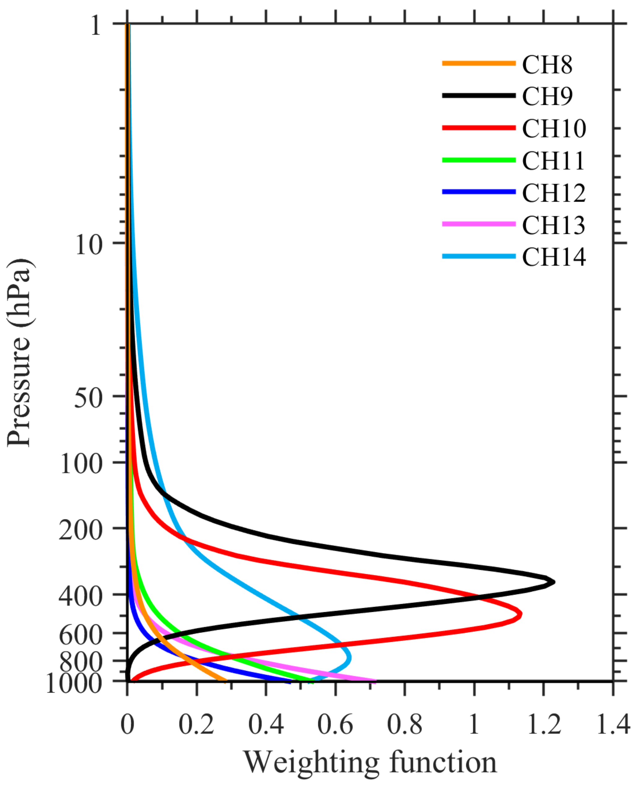
Figure 1. Weighting functions of FY–4A/AGRI infrared bands calculated using ARMS with the US 1976 standard atmosphere as the input.
Remotesensing 13 03120 g001
Figure 2. Observed brightness temperature distributions at ~3.75–μm for (a,c) FY–4A/AGRI band 8 and (b,d) Himawari–8/AHI band 7 (a,b) at 0600 UTC and (c,d) at 1700 UTC on 23 April 2019. (Unit: K).
Remotesensing 13 03120 g002
Figure 3. Frequency distribution of AGRI band–8 brightness temperatures within 2 K–intervals for all valid observations with satellite zenith angles less than 60° and over the ocean during 1500, 1600, 1700, 1800, and 1900 UTC in (a) January, (b) April, (c) July, and (d) October 2019. Note that no pixels with solar zenith angles less than 90° were observed at these hours.
Remotesensing 13 03120 g003
Figure 4. Time series of the number of AGRI pixels with observed band–8 brightness temperatures greater than 300 K during (a) 1600, (b) 1700, and (c) 1800 UTC for each day in 2019, respectively, as a percentage of the total number of pixels of the current time period. The gray bars in the figure indicate missing observations. Only pixels with a satellite zenith angle less than 60° and that were over the ocean were used. Note that no pixels with solar zenith angles less than 90° were observed at these hours.
Remotesensing 13 03120 g004
Figure 5. Distribution of clear–sky data counts (×103) for FY–4A/AGRI with satellite zenith angles less than 60° collocated with MODIS cloud mask products in January, April, July, and October 2019.
Remotesensing 13 03120 g005
Figure 6. (a,b) Mean biases and (c,d) standard deviations calculated by OMBARMS (orange) and OMBRTTOV (blue) with ERA5 data as input statistics for clear–sky data in January, April, July, and October 2019, over (a,c) the ocean and (b,d) land with satellite zenith angles less than 60°.
Remotesensing 13 03120 g006
Figure 7. Spatial distributions of OMBFNL biases of AGRI bands 8–14 with satellite zenith angles less than 60°, which are calculated within each 2° × 2° grid box in January, April, July, and October 2019. (Unit: K).
Remotesensing 13 03120 g007
Figure 8. Spatial distributions of OMBFNL biases for AGRI band 11 calculated within each 2° × 2° grid box in (a) January, (b) April, (c) July, and (d) October 2019, respectively. (Unit: K).
Remotesensing 13 03120 g008
Figure 9. Monthly mean biases of AGRI bands 8–14, calculated by OMBFNL statistics for data (a) over the ocean and (b) over land in January, April, October, and July 2019.
Remotesensing 13 03120 g009
Figure 10. Variations of (a) biases and (b) standard deviations of OMBFNL with respect to satellite zenith angles for AGRI bands 8–14 over the ocean in January, April, July, and October 2019. Data counts calculated at 2° intervals are indicated by grey shading in (b).
Remotesensing 13 03120 g010aRemotesensing 13 03120 g010b
Figure 11. Variations of (a,b) biases and (c,d) standard deviations of OMBFNL, as well as (e) data counts with respect to scene brightness temperature for AGRI bands 8–14 over the ocean in January, April, July, and October 2019.
Remotesensing 13 03120 g011aRemotesensing 13 03120 g011b
Figure 12. Mean biases of AGRI bands 8–14, calculated by OMBFNL (red) and OMBERA5 (blue) statistics for data (a) over the ocean and (b) over land in January, April, October, and July 2019, respectively.
Remotesensing 13 03120 g012
Figure 13. Spatial distributions of (a) OMBERA5, (b) OMBFNL, and (c) OMBERA5 minus OMBFNL for band 11, and (d) skin temperature differences between the FNL and ERA5 datasets (FNL minus ERA5) with AGRI observations under clear–sky conditions in January, April, July, and October 2019, within each 2° × 2° grid box (Unit: K).
Remotesensing 13 03120 g013
Figure 14. Vertical distributions of mean difference temperature (ΔT, left panel) and fractional differences of specific humidity (Δq/q, right panel) between the FNL and ERA5 datasets (FNL minus ERA5) using clear–sky data over the ocean within the AGRI observing domain (zenith angle less than 60°) at 0000, 0600, 1200, and 1800 UTC in January, April, July, and October 2019. The weighting functions for AGRI bands 9–10 are also shown (dashed curves).
Remotesensing 13 03120 g014
Table 1. Characteristics of FY–4A/AGRI infrared bands 1.
Channel (Band) No.Central Wavelength (μm)Spectral Interval (μm)SNR or NEdT Specified (km)Spatial Resolution at SSP (km)
73.753.5–4.00.7 K @ 300 K2
83.753.5–4.00.2 K @ 300 K4
96.255.8–6.70.3 K @ 260 K4
107.16.9–7.30.3 K @ 260 K4
118.58.0–9.00.2 K @ 300 K4
1210.810.3–11.30.2 K @ 300 K4
1312.011.5–12.50.2 K @ 300 K4
1413.513.2–13.80.5 K @ 300 K4
1 Data were provided by [44].
Table 2. Input variables and parameters for clear-sky simulations using ARMS or RTTOV.
CategoryVariable NameUnitData Resource
Atmosphere variableLevel and Layer PressurehPaERA5/ FNL
TemperatureK
Water Vapor Mixing Rationg/kg (kg/kg)
O3 Mixing Rationppmv
CO2 Mixing RationConstant (376)
Surface variablesSkin TemperatureKERA5/ FNL
Land Surface Emissivity--CAMEL_HSRemis
Ocean Surface Emissivity--Calculated based on Wu and Smith (1997) [46]
Wind Speedm/sERA5/FNL
Wind Directiondegree
Satellite GeometrySatellite Zenith AngledegreeDerived from FY–4A/AGRI L1 data with HDF format
Satellite Zenith Angle
Solar Zenith Angle
Solar Azimuth Angle
ParametersClimatology--US 1976 standard profile
Land Coverage--1 for land and 0 for ocean
Water Coverage0 for land and 1 for ocean
Snow CoverageAlways 0
Ice CoverageAlways 0
Table 3. Biases and standard deviations calculated by the differences in brightness temperature between AGRI observations and ARMS simulations using the FNL dataset as the background for data under clear–sky conditions and with satellite zenith angles less than 60° in January, April, July, and October 2019.
Channel No.OceanLand
μ (K)σ (K)μ (K)σ (K)
80.221.000.124.99
91.061.200.701.44
100.691.040.651.52
11−0.691.250.194.55
12−0.611.160.325.18
13−0.411.240.324.98
140.411.320.752.87
Publisher’s Note: MDPI stays neutral with regard to jurisdictional claims in published maps and institutional affiliations.