Article

A Framework for Actual Evapotranspiration Assessment and Projection Based on Meteorological, Vegetation and Hydrological Remote Sensing Products

College of Water Sciences, Beijing Normal University, Beijing 100875, China
*
Author to whom correspondence should be addressed.
Remote Sens. 2021, 13(18), 3643; https://doi.org/10.3390/rs13183643
Submission received: 11 July 2021 / Revised: 6 September 2021 / Accepted: 10 September 2021 / Published: 12 September 2021

Abstract

:
As the most direct indicator of drought, the dynamic assessment and prediction of actual evapotranspiration (AET) is crucial to regional water resources management. This research aims to develop a framework for the regional AET evaluation and prediction based on multiple machine learning methods and multi-source remote sensing data, which combines Boruta algorithm, Random Forest (RF), and Support Vector Regression (SVR) models, employing datasets from CRU, GLDAS, MODIS, GRACE (-FO), and CMIP6, covering meteorological, vegetation, and hydrological variables. To verify the framework, it is applied to grids of South America (SA) as a case. The results meticulously demonstrate the tendency of AET and identify the decisive role of T, P, and NDVI on AET in SA. Regarding the projection, RF has better performance in different input strategies in SA. According to the accuracy of RF and SVR on the pixel scale, the AET prediction dataset is generated by integrating the optimal results of the two models. By using multiple parameter inputs and two models to jointly obtain the optimal output, the results become more reasonable and accurate. The framework can systematically and comprehensively evaluate and forecast AET; although prediction products generated in SA cannot calibrate relevant parameters, it provides a quite valuable reference for regional drought warning and water allocating.

1. Introduction

Since 2020, southwestern California in the United States; Argentina and Brazil in South America; and many countries in Africa and western Europe have suffered from scarce rainfall and severe droughts, which has caused widespread concern. Actual evapotranspiration (AET) is a dominant reason for water loss in arid regions. It denotes the water that evaporates from the soil, vegetations, and water bodies to the atmosphere, driven by solar radiation and thermal dynamic processes [1,2,3]. Furthermore, AET is also an important part of the water cycle and energy exchange [4,5]. It is of great significance to evaluate and predict AET for drought warnings.
The evapotranspiration process involves water exchange and energy transfer among soil, water, atmosphere, and vegetation systems, which is difficult to estimate due to complicated mechanisms and sophisticated factors [6,7,8]. At present, AET is usually calculated by the evapotranspiration model based on the water balance method, energy balance system, and empirical coefficient [9,10]. Tandogdu and Camgoz [11] calculated the soil transpiration factor based on experimental data and estimated AET in combination with aerodynamic methods. Jin et al. [9] estimated AET in eight hydrological regions in Northwest China through Surface Energy Balance Algorithm for Land (SEBAL) [12]. Miao et al. [13] used the water balance equation to calibrate the parameters and combined with the Generalized Complementary Principle [14] to estimate the AET in Huaihe River Basin. Chen and Xu [15] evaluated the performance of seven evapotranspiration models in the aspect of water balance research. Rana and Kater [16] summarized 10 empirical methods for measuring and estimating AET. Sarma and Bharadwaj [17] evaluated eight evapotranspiration models based on crop coefficients and concluded that the Penman-Monteith [18] and Priestly-Tailor [19] models were more effective. However, these previous traditional methods mainly used empirical coefficients to explain the complex mechanism to a certain extent, and field measurement data seemed to have become an indispensable part [20]. As a result, they can only accurately evaluate the homogeneous area near the meteorological station, and it is not feasible to measure evapotranspiration in a wide range of areas in practice and economy [15,21].
Fortunately, the emergence of remote sensing technology has filled the gap in areas poorly monitored [21]. Moene et al. [22] input satellite data into SEBAL to estimate the AET in central Bolivia. Similarly, Tim et al. [23] and Tofigh et al. [24] used Landsat imagery and MODIS imagery combined with weather data to estimate AET through the SEBAL algorithm, respectively. By using multi-source satellite data to measure the required surface and meteorological variables, the accuracy and spatial description of actual evapotranspiration are significantly improved [25]. On top of that, GLDAS combines satellite and ground observation data to produce a high-precision global AET data set using land surface models and data assimilation technology, which has become an important data source for global changes and hydrological cycles [26,27,28]. Andam et al. [29] applied the GLDAS AET to the Votla watershed in Africa and found that it was more consistent with the overall average evapotranspiration produced by various products. Muhammad et al. [30] evaluated uncertainty of three AET products—GLDAS, GLEAM, MODIS—through an extended triple collocation approach and found that GLDAS showed the least absolute uncertainties and highest accuracy in Asia. Muhammad et al. [31] also found that GLDAS AET shows the best performance among the four AET datasets (MOD16, GLEAM, GLDAS, and AWRA-L) according to in-situ flux tower measurements in Australia. Although there is a little uncertainty, the overall accuracy of GLDAS AET is relatively high and can be used to analyze evolution characteristics [32]. Furthermore, the rise of machine-learning algorithms allows scholars to avoid the exploration of complex mechanisms and obtain valuable evaluation results directly through sufficient relevant parameters [33,34]. Filgueiras et al. [35] applied vegetation index and random forest algorithm to effectively predict Brazil’s water-management parameters. Shrestha and Shukla [36] found that the accuracy of using support vector machines to predict crop coefficients and AET is 49.3 mm higher than the FAO-56 method. Regrettably, since a machine learning algorithm is an arduous task that spends a great deal of time and effort to select optimal parameters, there are few results concerning the use of multi-source remote sensing data combined with machine learning algorithms to evaluate AET for the time being.
As for input variables, previous studies introduced remote sensing products expressing vegetation growth and coverage information into the prediction model of AET, which effectively increased the accuracy of the model [37,38]. This study attempts to add hydrological factors closely related to the evaporation process—total water storage and runoff—so as to further improve the accuracy. About the machine-learning model, random forest model is not sensitive to missing data, which solves the problem of simulation and prediction in the case of missing data in a small-scale area [39,40]. Support vector machine classification is simple and effective and can solve the problem of a nonlinear relationship with different kernel functions [41]. This study intends to apply these two methods, compare and evaluate their results, and further try to combine them to produce a set of optimal AET products.
Hence, this study aims to design a data-driven structure based on multi-source remote sensing data and machine learning algorithms to systematically evaluate and predict AET. Specifically, we ask the following research questions:
  • How does actual evapotranspiration dynamically evolve?
  • What are the relevant and decisive factors that affect the AET changes?
  • What kind of input and which machine learning algorithms can simulate the most intense future AET?
  • How to integrate the results of multiple machine learning algorithms to generate an optimal set of AET future prediction products?

2. Materials and Methods

2.1. Case Study

In order to apply the framework proposed in this study, we chose South America as the study area. South America (SA) has a total area of 17.84 million square kilometers, with the range of 34°36′W–81°20′W and 53°54′S–12°28′N, making it the fourth largest continent by land area (Figure 1).
SA has the largest tropical rain forest in the world—the Amazon rainforest, whose rainfall is the most abundant in the world [42]. However, river records show that the region experiences an extreme climate event flood or drought every 10 years on average [43]. The typical climate type, tropical rainforest and tropical grassland climate, as well as the well-known El Niño phenomenon, cause intense hydrological processes in SA [44,45]. The sufficient evaporation conditions, severe hydrological cycle, and typical climate characteristics also bring the risk of excessive evapotranspiration. Many scholars have predicted that droughts will increase in parts of South America in the future [46,47].

2.2. Data

2.2.1. Meteorological Data (Temperature, Precipitation, and Potential Evapotranspiration)

Meteorological data including monthly average gridded daily mean temperature (T), precipitation (P), and potential evapotranspiration (PET) with a spatial resolution of 0.5 degrees are obtained from the Climate Research Unit (CRU) Version 4.05. Retrieved from monitoring data from meteorological stations, data developed by CRU is widely used in the field of climate change [48].
Table 1 summarizes the details of the data used in this study.

2.2.2. Hydrological Data (Actual Evapotranspiration, Total Water Storage, and Runoff)

As an important limiting factor and result of AET, the changes of terrestrial water storage (TWC) data obtained from the Gravity Recovery and Climate Experiment (GRACE) and its following project GRACE-FO are used to assess AET. Launched in 2002, the GRACE project transformed the gravity and mass variations to produce TWC data [49]. This study used the monthly dataset of JPL GRACE(-FO) RL06 mascons with a spatial resolution of 0.5 degrees.
As another important part of the hydrological cycle, the amount and velocity of runoff also affect the regional water surface evaporation. Integrating satellite- and ground-observed data, the Global Land Data Assimilation System (GLDAS) aims to simulate high-resolution global land hydrology and energy flux through global land surface models, which is highly recognized and widely used in hydrology [26,27,28]. The actual evapotranspiration (AET), surface (Qs), subsurface (Qsb), and snowmelt runoff (Qsm) simulated by the Noah model with the spatial resolution of 0.25 degrees were employed in this study. The equation of the total runoff can be expressed as:
R = Q s + Q sb + Q sm
where R represents the total regional runoff.

2.2.3. Vegetation Index (NDVI)

The monthly Normalized Difference Vegetation Index (NDVI) dataset with 0.05 degrees spatial resolution was derived from the MODIS. The version is MOD13C2 Version 6. NDVI dataset developed by MODIS is generally applied in botany and ecology to reflect the temporal and spatial characteristics and dynamic changes of vegetation [50,51].

2.2.4. Future Climate Scenarios (CMIP6)

The datasets of future climate scenarios derived from the Coupled Model Intercomparison Project (CMIP) were forced into RF and SVR models to predict the future AET in South America. The recent model outputs from CMIP6 promise to provide the most reliable future climate predictions due to the massive improvements in the physical chemistry processes [52,53,54]. The monthly T and P datasets developed by the Nation Center for Atmospheric Research (NCAR), and the monthly PET datasets estimated by the Institut Pierre-Simon Laplace (IPSL), with the resolution of 100 km and 250 km from 2020 to 2090, respectively, were employed in the study. The Representative Concentration Pathways 4.5 corresponding to the SSP245 was treated as a stabilization pathway in the present study, representing atmosphere radiation at 4.5 Watts/m2 at the end of 2100 [55].

2.3. Methods

2.3.1. Man-Kendall Test

Recommended by the WMO, the Mann–Kendall (MK) test is widely used as a nonparametric test of temperature, precipitation, and other factors [56]. The advantage is that the samples do not need to follow a certain distribution and are not disturbed by small fluctuations. The MK test can also reveal the trend and mutation of a dataset [57].
A statistical value Z is defined, and the detailed calculation process can be seen in Liu et al. [58]. Z is an indicator for the severity of the changing trend. The positive value indicates that the trend is rising, while a negative value indicates that the trend is falling. If | Z | | Z ( 1 α ) / 2 | , it means that at an α significance level, the data series changes significantly.

2.3.2. Boruta Algorithm

Boruta Algorithm is an effective method for optimizing attribute selection, which is widely used in many research fields [59,60]. By randomly designing shadow features for all the considered candidate features, it can capture all the relevant features in the dataset and rank the relative importance of the features [28,61]. The important value of shadow features determines whether candidate features are further selected. The main calculation steps are as follows:
  • Copy all features to build random shadow features. Shuffle all the features in the data randomly and rearrange the order of the features.
  • Input the features and their copies into the random forest classifier to calculate the Z-scores.
  • Remove features with lower Z-scores than the shadow attributes. The important variables, whose Z-scores are over the set of shadow features, are verified.
  • Repeat steps 1–3 until all variables are identified.
In this paper, the package “Boruta” in R software [62,63] was used to filter the most essential factors of AET. More specific instructions of the Boruta Algorithm can be found in Kursa and Rudnicki and Qu et al. [61,64].

2.3.3. Support Vector Regression (SVR)

Support vector machine (SVM) is a powerful method in statistical machine learning [41,65]. As an extension of SVM, a more robust support vector regression (SVR) model has been successfully employed to the prediction of time series [66,67].
The problem of linear SVR can be formalized as:
m a x 1 2 ω 2 s u b j e c t   t o     | f ( x i ) y i | ϵ ,     i = 1 , 2 , , N
where x i is the training point in the total sample of size N , and y i is the true value corresponding to x i ; while f ( x i ) is the predictive value and f ( x ) = ω x + b , it assumes that the SVR model can only tolerate deviations that do not exceed ϵ between f ( x i ) and y i . Then, two slack variables ξ i , ξ i ^ 0 are introduced for each sample point to make the constraint become ϵ + ξ i ξ i ^ , where ξ i and ξ i ^ represent the degree of unsatisfying constraints, consequently, the SVR model evolves into:
m a x 1 2 ω 2 + C i = 1 N ( ξ i + ξ i ^ )   s u b j e c t   t o f ( x i ) y i ϵ + ξ i y i f ( x i ) ϵ + ξ i ^ ξ i , ξ i ^ 0 ,       i = 1 , 2 , , N
where C is a constantly called box constraint, which represents the penalty for misclassification. The Lagrange multiplier α i and α ^ i are introduced to transform Equation (3) into a dual optimization problem. The final classification decision function can be written in the following dual form:
f ( x ) = i = 1 N ( α ^ i α i ) ( x x i ) + b
The dual form of SVR of nonlinear function is:
f ( x ) = i = 1 N ( α ^ i α i ) K ( x , x i ) + b
where K ( x , x i ) = ϕ ( x ) ϕ ( x i ) is the kernel function. In the current paper, the tool “fitrsvm” in MATLAB 2020b was applied to perform the SVM in the pixel scale in the world. Besides, the historical datasets of each pixel were randomly divided into 70% as the training set, and the rest as the test set. The determination coefficient ( R 2 ) was utilized to test the accuracy of SVR.
R 2 = 1 i = 1 N ( y ^ i , t e s t y i , t e s t ) 2 i = 1 N ( y ¯ i , t e s t y i , t e s t ) 2

2.3.4. Random Forest (RF)

Random Forest (RF) is a popular machine-learning algorithm that can be used to construct classification and regression problems [68,69]. It has many advantages, (1) it can automatically divide features; (2) it is not sensitive to missing data, that is, it can maintain high accuracy in the case of a large number of missing data; (3) it can effectively avoid overfitting and has good performance in small-scale data sets [39,40].
More details about random forests can be found in Arlot and Genuer [70]. In this study, we utilize the “Treebagger” tool in MATLAB 2020b to implement the RF on the pixel scale and find the optimal node number and leaf number of each pixel.

2.3.5. Research Framework

Figure 2 depicts the framework proposed in this study to evaluate and predict AET using multi-source remote sensing data. After the data is prepared, the MK test is performed on the pixel scale to calculate the statistical value Z of the AET and the climate tendency rate is calculated through linear regression, and then the calculation results are analyzed and displayed in space. This is the technological process of the evolution assessment, which is a common, basic data evaluation and overview process. Furthermore, the temporal and spatial resolution of meteorological data, vegetation data, and hydrological data are unified to 0.5-degree spatial resolution. In this study, we adopt the mean pixel aggregation and resampling method to upscale the image [71], and the “Imresize” tool in MATLAB 2020b combined with Bicubic interpolation method is employed to downscale. Pearson correlation analysis [28] and Boruta algorithm are used to evaluate the Pearson correlation coefficient and dominant factor order of AET change. This is the procedure of relevant and dominant assessment, whose results can make an important reference for the next part in terms of machine learning classification. Thirdly, combined with the future climate dataset, different forecast input strategies are divided according to the data characteristics or the actual situation, and the AET of each input strategy is predicted by RF and SVR on the pixel scale. To obtain the reliable machine learning model, the training set (the sample size accounts for 70% of the original) and the testing set (30%) are divided randomly. Further, we use the ‘fitsvm’ tool in MATLAB R2018b to automatically optimize the hyperparameters of the support vector machine model and the ‘TreeBagger’ tool in MATLAB R2018b to determine the optimal number of leaf nodes and learners for the training set. After gaining the optimal machine learning model, the testing set are used to test the model. Then, by calculating the model’s determination coefficient R 2 , average absolute error (MAE), and root mean square error (RMSE), the simulation accuracy of the two models is compared. Finally, the prediction result of the model with higher simulation accuracy is selected as the final prediction result for each grid to generate the joint optimal projection.
In this study, South America is selected as the case study to apply the framework and determine its advantages and disadvantages.

3. Results

3.1. Assess the Evolution Tendency of AET

3.1.1. Temporal Evolution

The monthly average AET of South America is 87.88 mm; the amplitude of AET is not large during the year (Figure 3a). From 2002 to 2020, the annual AET in South America was between 1003.96–1102.78 mm, which generally increased at an average rate of 43.4 mm every 10 years, but the AET dropped sharply in 2020 (Figure 3b). Furthermore, the statistical value Z from the MK test of annual AET is 3.08, indicating a significant increasing trend (Z > 1.96, α = 0.05). Table 2 shows the tendency of monthly AET in South America from 2002 to 2020. The Z value of each month is greater than 0, showing an increasing trend. Except for August to November, the increasing trend is quite significant.

3.1.2. Spatial Evolution

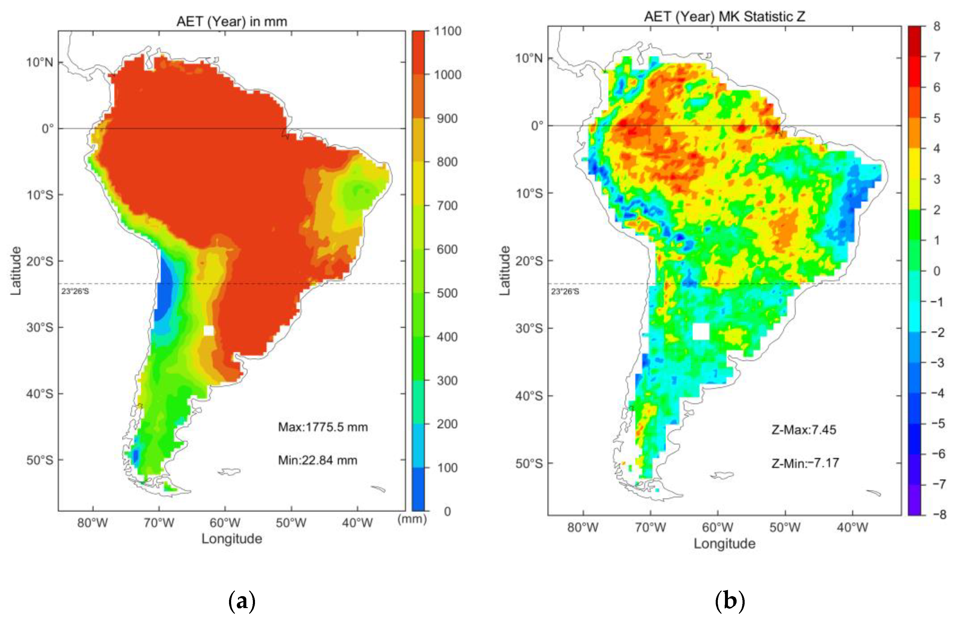
The spatial distribution of AET in South America roughly presents a low distribution on both sides while the high in the middle, and the high-value area (>1000 mm) has a large range (Figure 4a). In the eastern Cape Branco and the western and southern plateau areas, the AET is less than 600 mm; especially in the vicinity of the Yuyeyaco Volcano near the equator, the AET reaches the lowest value of less than 200 mm. In addition, the tendency of annual AET also presents a similar scene (Figure 4b). In the east and west coasts within the equator and the Tropic of Cancer, there is a relatively concentrated area of AET exhibiting a downward trend. It is worth noting that the Z value even exceeds four in the north of the tropic line, especially the large area in the middle and upper reaches of the Amazon, which illustrates a significant increase.
In order to further evaluate the spatial distribution of AET, the map of AET and its Z value in the four seasons are depicted in Figure 5 and Figure 6, respectively. The spatial distribution of September to November and December toFebruary is consistent with the annual AET (Figure 4a). The average AET of the Amazon Plain and the northern regions were relatively stable, and they were always greater than 300 mm in the four seasons (Figure 5). Figure 6 illustrated the increasing trend of AET in most parts of South America (Z > 0), with a decreasing trend only in coastal areas and southern regions in the four seasons. Remarkably, the range of high-value areas in South America from December toFebruary and March toMay is relatively large (Figure 5a,d), and the scale of the high Z value from MK during the two periods is also large (Figure 6a,d), which indicates a large-scale increasing trend of AET in the middle and upper reaches of the Amazon River and most parts of Brazil. The relevant government departments need to pay more attention to the fact that large areas of high AET may cause severe droughts.

3.2. Assess the Relevant Factors and Determinant Order of AET

Pearson correlation coefficient (P-Coefficient) and Boruta algorithm based on RF were used to calculate the correlation and determinant order of influencing factors for monthly AET. Table 3 shows the correlation and determinant order assessment results for the entire region of South America. The correlation between the six factors and AET is all promotion (P-coefficient > 0). Among them, the correlations between T, P, NDVI, and AET are more significant, and the relationship between R and AET is the smallest. The determinant order obtained by Boruta is almost the same as the size ranking of the P-coefficient, but the two differ in the decisive order of PET and TWC. Although the P-coefficient of TWC is larger, the Boruta algorithm shows that the decisive order of PET is higher.
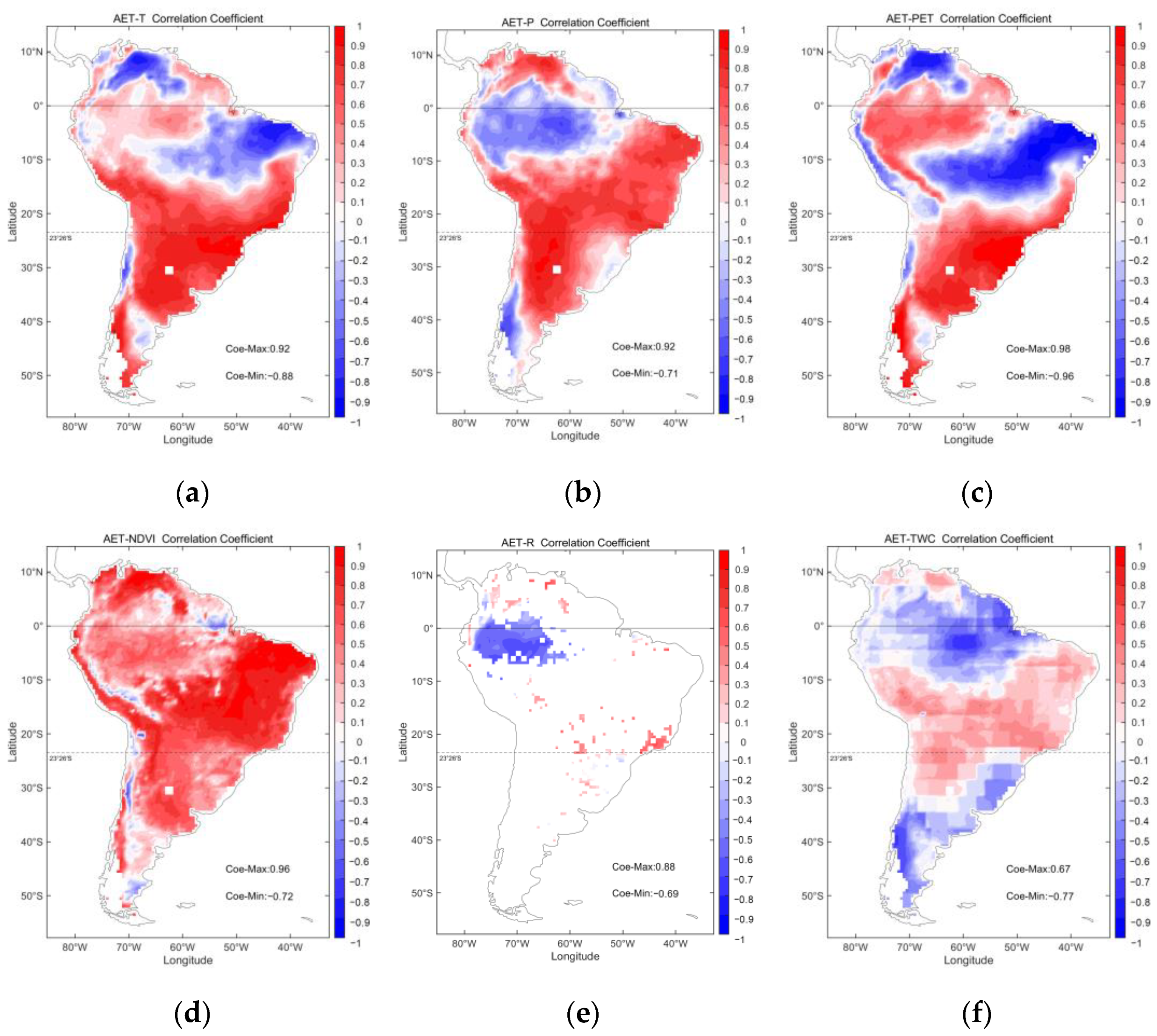
Further, the P-coefficient and determinant order between monthly AET and each grid were evaluated on the pixel scale. Figure 7 shows the spatial distribution of the P-coefficient between AET and each factor. By comparison, the correlation between hydrological factors is the weakest, especially it only displays a negative correlation with R in the middle and upper reaches of the Amazon Plain, which indicates that the rapid runoff here may inhibit AET (Figure 7e,f). As a result of the AET process, there is a slight positive correlation between TWC and AET in Central South America. It is unreasonable that TWC increases along with the raise of AET. The increase in TWC and AET may be more closely related to other factors such as increased precipitation. In addition, the whole district consistently exhibits the positive correlation between NDVI and AET (Figure 7d). AET is positively correlated with T and P in most parts of the region, but abnormally, the negative correlation about T emerges in the northern plateau of Brazil and the plateau area north of the equator, while the negative correlation about P occurs in the Amazon plain.
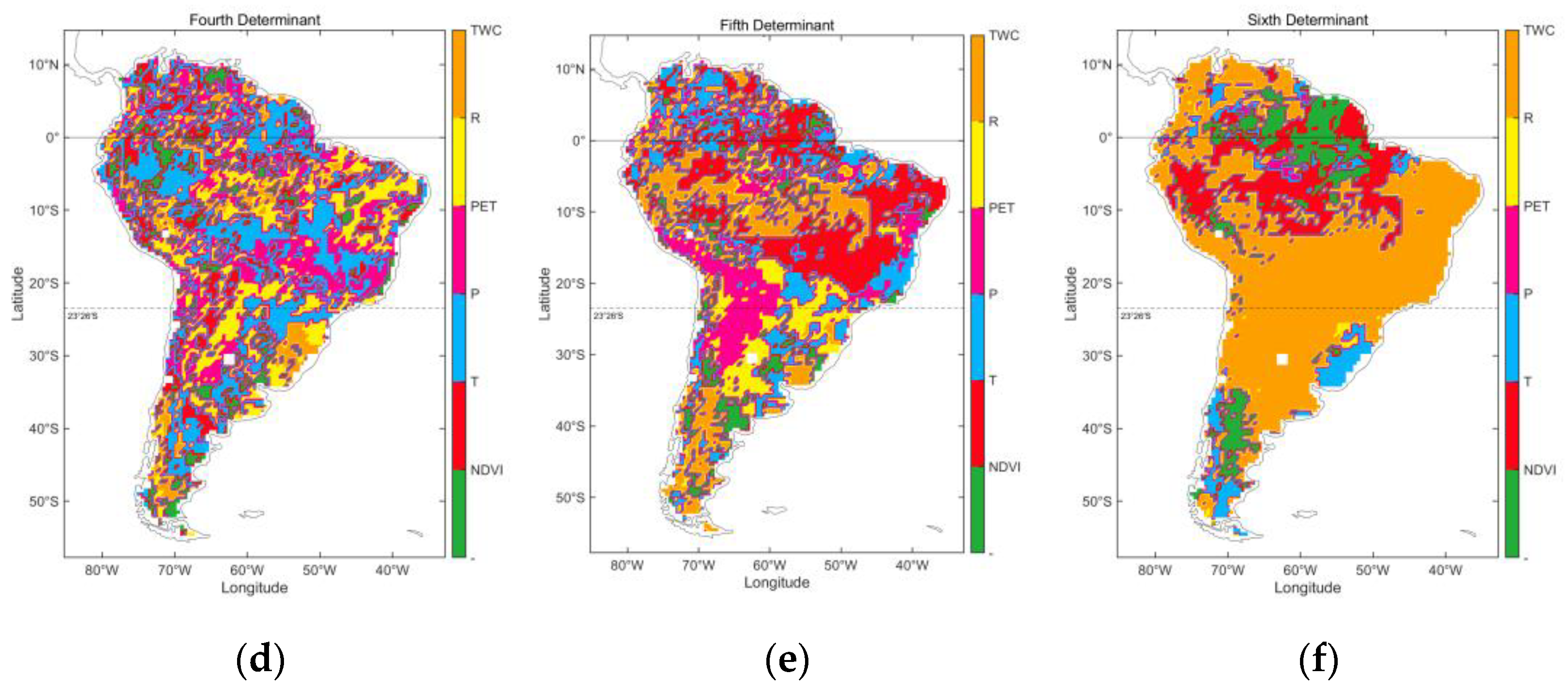
Figure 8 depicts the map of the decisive factors at each order from Boruta algorithm. The distribution of the primary determinant and the weakest determinant is relatively uniform and concentrated, while the distribution of the second-fifth determinants is relatively sporadic. With the largest proportion (24.85%) in the first determinant factor (Table 4), NDVI is mainly distributed in the Brazilian plateau (Figure 8a). In addition, Table 4 shows that the proportion of PET in the top three order determinants exceeds 20%, which can be attributed to the fact that PET is a reference used to estimate AET. In addition, Figure 8a shows that the reference value of PET is relatively significant in the Pampas and Parana plateau areas south of the Tropic of Capricorn. Notably, the proportion of R also exceeds 20%, and it is the primary determinant in the upper and middle reaches of the Amazon plain (Figure 8a). Considering the strong negative correlation between R and AET, it can be speculated that fast and abundant runoff is the main factor inhibiting AET in the Amazon region.

3.3. Projection of AET under Different Input Strategies

3.3.1. Accuracy of the Models under Different Input Strategies

This study divided three prediction input strategies by gradually inputting different types of variables. The specific details of the input variables for the three input strategies are shown in Table 5. In the three input strategies, the future AET is simulated by RF and SVR on the pixel scale in South America. Considering the limitation of computational efficiency, the machine learning model is performed at a spatial resolution of 1 degree. This study ran machine learning models with different input strategies on the grid scale and calculated their R 2 . Table 6 shows the proportion of grids that R 2 exceeds 0.9, 0.7, and 0.5, respectively. R 2 is a common performance measurement index in the machine learning model. The closer R 2 is to 1, the closer the predicted value and the true value in the test set sample are, that is, the higher the accuracy and the better performance of the model [72]. On the whole, the area with R 2 > 0.5 accounts for more than 50% of the total area, indicating that the model can predominantly explain the AET in half of South America. From the comparison of the three input strategies, by gradually increasing the input variables, the R 2 of the model is continuously improving, especially after considering the NDVI, the accuracy of the model is significantly improved (Table 6). In each input strategy, for R 2 at the same level, the proportion of the RF model is greater than the SVR model in three input strategies, which demonstrates that the RF model is suitable for more regions in South America.
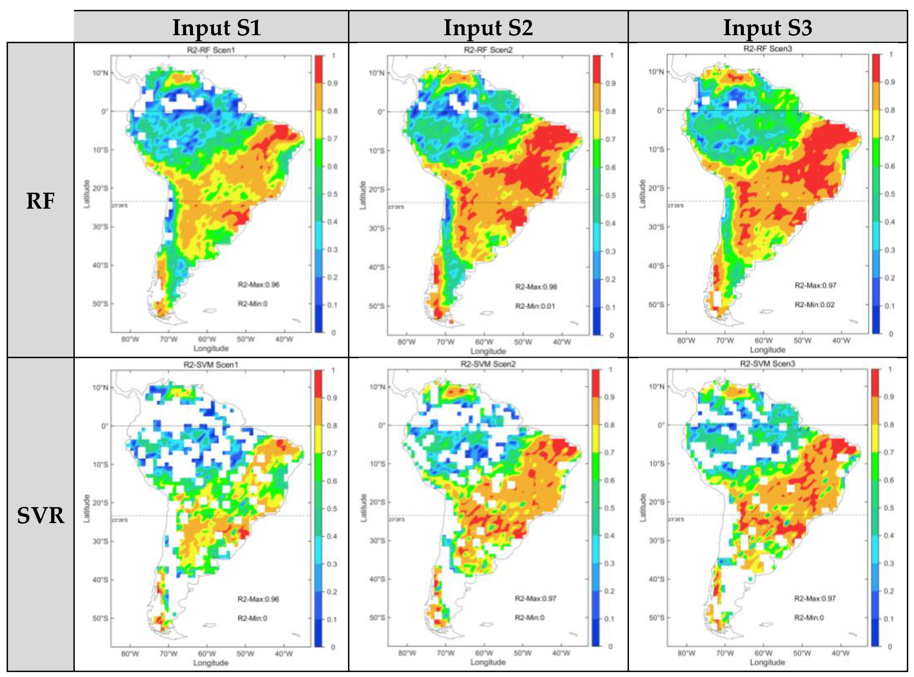
Furthermore, Figure 9 depicts the spatial distribution of R 2 , it can be seen that RF is more suitable for the entire South American region. With R 2 even less than 0.1, the SVR performs poorly in the Amazon plains and the high plateaus of Brazil. In addition, regarding the difference between input strategies, compared to S1, the RF model has a greater improvement in S2 and S3, especially in Brazil. To further test the accuracy of the model, Figures S1 and S2 (in Supplementary Materials) depict the MAE and RMSE of each input strategies, which also express the smaller MAE and RMSE, relatively, in S2 and S3. In addition, the MAE and RMSE of the RF model in the three input strategies are the smallest (both between 0 and 0.03), and the maximum MAE of S2 is only 0.02. The results of SVR show that from S1 to S3, as the inputting variables increase, the MAE and RMSE of the model become smaller and smaller, and the accuracy of the model gradually improves.

3.3.2. Joint Optimal Prediction of Two Models

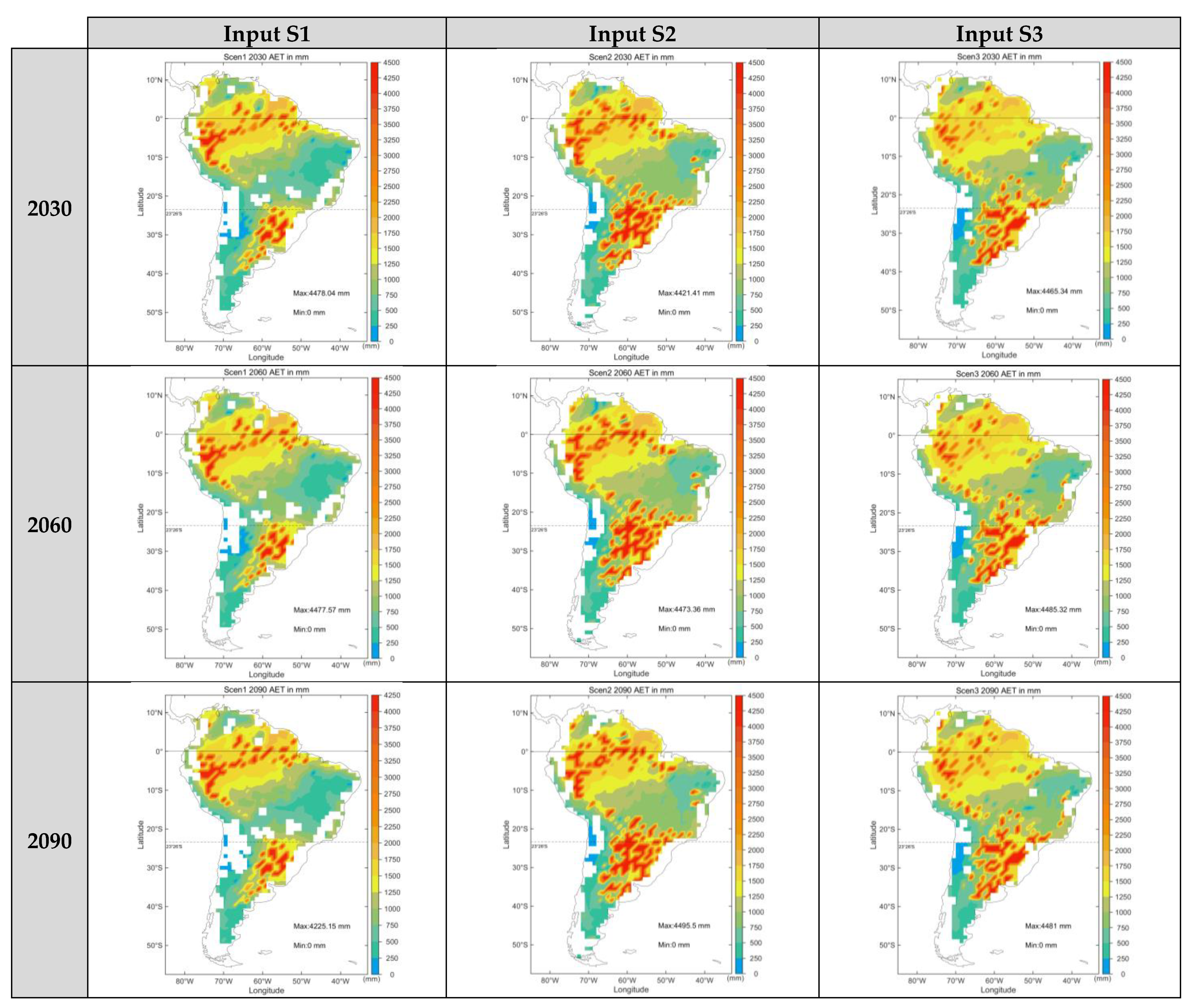
Although we concluded that RF is more applicable to the prediction of AET in South America in the previous section, SVR may perform better in a few individual regions. We compared the R 2 of the two models for each grid for the three input strategies, so as to evaluate the results of the two models more comprehensively. We chose a model with a larger R 2 to predict AET from 2030 to 2090, and developed a set of optimal AET prediction products for the three input strategies, with a spatial resolution of 1 degree and a temporal resolution of monthly scale. The product data format is ‘NetCDF’, which is available in the Supplementary Materials. Figure 10 expresses the annual AET values for 2030, 2060, and 2090 calculated by the joint optimal prediction value on a monthly scale. From the vertical axis in Figure 10, the spatial distribution of the simulation results is roughly the same in each input strategy, and this distribution would not change over time. All three input strategies predict unusually severe droughts in the Amazon region and some areas south of the Tropic of Capricorn from 2030, which implies that the relevant departments need to take some measures about water resource management to ensure the progress of agricultural activities in these areas. In the three input strategies, it can be found that S2 considering climate and vegetation factors can simulate a larger range of intense AET values (Figure 10).

4. Discussion

4.1. The Framework of Trend Assessment

The trend assessment framework was applied to South America to explore the trend evolution and distribution of AET, and we found that the evapotranspiration in South America expressed an upward trend from 2002 to 2020, especially quite significantly in the area north of the equator, which was consistent with many previous studies [46,73,74,75,76]. Yang et al. believed that climate warming led to an increase in the demand for atmospheric evaporation [73]. Elder et al. further found that the increase of AET in the equatorial region of South America may be related to the positive phase effect of the multi-decadal turbulence in the Atlantic Ocean [74]. In addition, we found a sharp drop in AET in 2020 (Figure 3b). Considering that South America experienced severe droughts and rare precipitation throughout the region, especially Brazil, Argentina, and Chile, in those places that suffered from a serious shortage of precipitation in 2020, it could be speculated that insufficient moisture will be the main limiting factor for AET in 2020.

4.2. The Framework about the Relevant and Dominant Factor Assessment of AET

The relevant and dominant factor assessment system combining P-coefficient and Boruta algorithm proposed in this study was utilized in South America as a case. It was found that T, NDVI, and P have a strong leading role in South America. What is more, it is consistent with existing research results that show T and P as the main driving factors of evapotranspiration in South America [73,77]. Unexpectedly, as the reference value of AET, PET was not very closely relevant in South America (P-coefficient only 0.587). This may be related to the poor adaptability of the PET estimation method in this area. The PET dataset was from CRU developed by Penman–Monteith formula, however, Martinez and Thepadia compared various methods of estimating PET and found that Penman–Monteith formula performed the worst in Florida (a city adjacent to the South America) [78]. Remarkably, the whole region consistently exhibited a positive correlation between NDVI and AET (Figure 7d), which resembled the results demonstrated by Ghilain et al. [79] and Costa et al. [80], in that AET highly depended on vegetation dynamics in South America. In addition, we found that AET increased in central South America, and TWC increased, which was illogical because TWC was induced by AET. It implied that the increase in water volume or the increase in AET may be more closely related to other factors such as the precipitation. Zhang and Cai also have similar findings [81]. In summary, after inputting MODIS NDVI and GRACE TWC, the evaluation framework found remarkable results in South America, which is reasonable and can be reflected by other research findings.

4.3. The Framework about the Joint Optimal Projection of AET

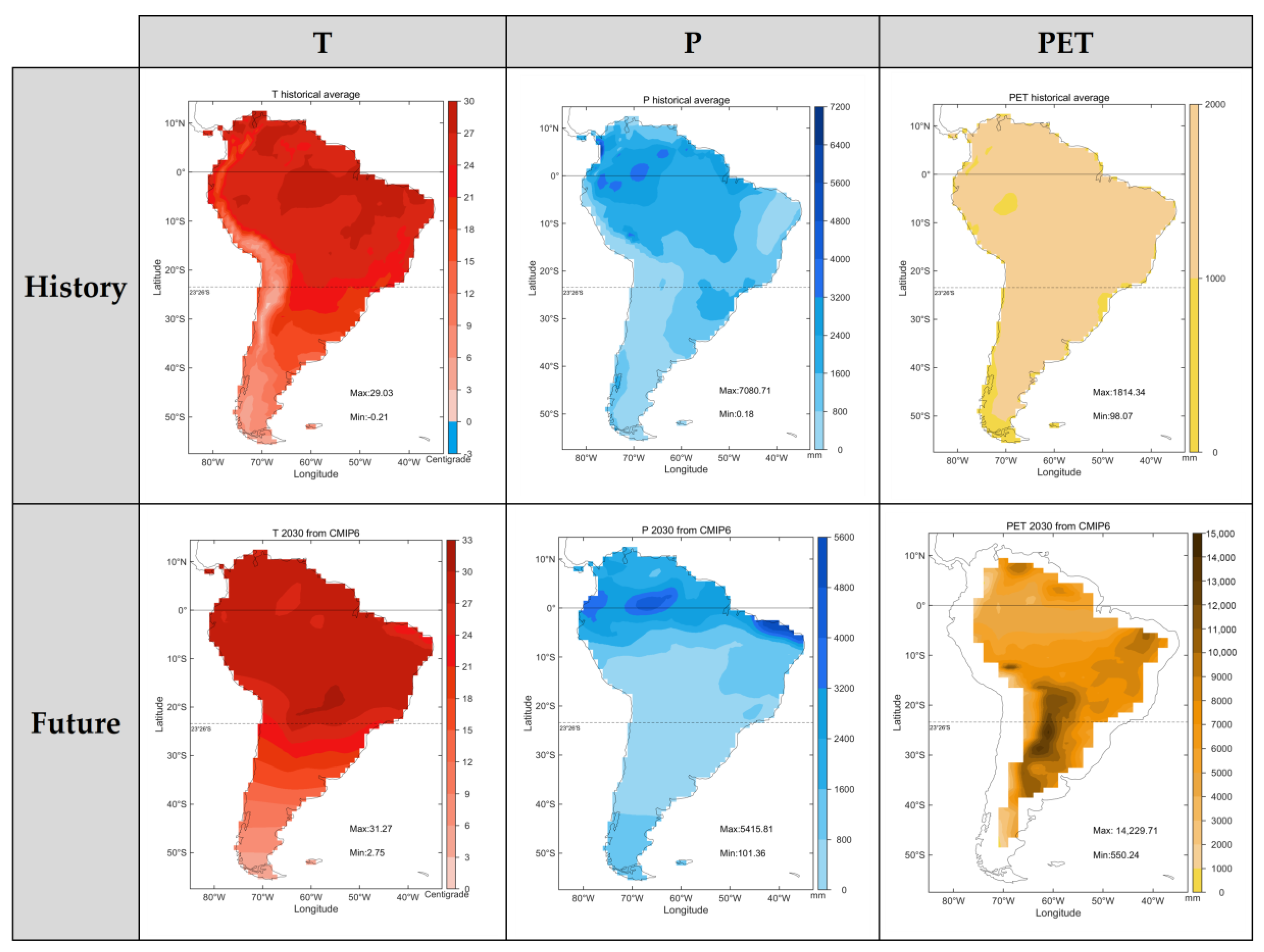
It was noteworthy that the three input strategies all predicted abnormally severe droughts in the Amazon region and parts of the south of the Tropic of Capricorn. The predicted AET was twice the current amount, and it was even three to four times in some areas. Although Thaler et al. and Lyra et al. also predicted a similar strong future evaporation here [82,83], we further clarified the causes of outliers. We doubted the input data given by CMIP6, because the AET doubled in the S1 only considering meteorological factors. Figure 11 compared the data from CMIP6 in 2030 with the historical multi-year average of CRU products. Obviously, the PET data from CMIP6 was flawed in completeness and magnitude. Nevertheless, even when the input CMIP6 PET had such an abnormal prediction value, the joint optimal result obtained by the framework proposed in this study reduced this abnormality. One reason may be the fact that PET ranked fourth in the decisive order of AET among all input factors (Table 3). Another may be that the multiple parameters input in this study could enhance the robustness of the model to a certain extent.
The framework proposed in this study can systematically and comprehensively evaluate the evolution and future trends of AET. This framework had three advantages: (1) It could comprehensively determine the order and distribution of the relevant and dominant factors that affected AET changes. (2) The input of multiple parameters also enhanced the robustness of the model, especially after the input of NDVI, avoiding large deviations in the outputs caused by a certain abnormal input parameter. (3) It coupled the prediction results of multiple machine learning models to make the results more reasonable and accurate. However, this study also had some limitations. On the one hand, this article only selected two more typical models with high recognition, and more models could be introduced into the framework in the future. On the other hand, it was found that there is a magnitude difference between the PET from CMIP6 and the current. However, due to the scarcity of available substitutes for this data set, we are restricted from further improving the prediction system. Similar to the function of the CMIP6 datasets, the South American AET forecast products developed in this case study under the three input strategies cannot be employed to quantify the other parameters, but they can serve as a valuable reference for the allocation of inter-regional water resources.

5. Conclusions

This research proposed an assessment and prediction framework for AET, which mainly relied on multiple currently popular machine learning models and multi-source remote sensing data. In order to present the algorithm more clearly, we applied the framework as a case study in South America and obtained the main conclusions as follows:
  • In South America, AET increased significantly at a rate of 43.4 mm/10a recently and experienced an obvious decline in 2020 due to water shortage. In terms of spatial distribution, AET values tended to be lower on both sides while higher (>1000 mm) in the middle. AET in most areas of SA exhibited a significant ascending trend, especially in the Amazon area.
  • With the P-coefficient exceeding 0.8, the correlation between AET and T, P, and NDVI was closer. The decisive factors obtained by Boruta algorithm were ranked as T > NDVI > P > PET > TWC > R, and NDVI controlled the largest area range. However, R was the primary determinant in the upper and middle reaches of the Amazon. It could be concluded that rapid runoff is the limiting factor for AET here due to the negative correlation.
  • SVR paled in comparison to the RF in South America. By comparing the R 2 of the two models on the pixel scale and selecting the optimal model for simulation, the joint optimal prediction datasets were obtained. Furthermore, the S2 considering meteorological and vegetation data derived from MODIS simulated the most intensive future evaporation in the three input strategies.
The framework developed in this study performed well in trend assessment and related determinant factor identification. The method, which combines multiple parameter inputs and two models to obtain the optimal output, could enhance the robustness of the model and make it more reasonable and precise. Limited by the lack of substitutes on the PET prediction dataset from CMIP6, the AET prediction products generated in South America in this study could not calibrate relevant parameters, but could provide a valuable reference for regional drought warning and water resources management.

Supplementary Materials

The following are available online at https://www.mdpi.com/article/10.3390/rs13183643/s1, Figure S1. Distribution of the simulation accuracy MAE of two models under different input strategies. Figure S2. Distribution of the simulation accuracy RMSE of two models under differ-ent input strategies. The AET prediction products generated in South America in this study.

Author Contributions

Conceptualization, Y.L. and Q.Y.; methodology, Y.L. and Q.W.; software, Y.L.; validation, Y.L., Q.Y. and Y.Z.; formal analysis, X.Y.; investigation, S.X.; resources, J.Y.; data curation, X.Y.; writing—original draft preparation, Y.L.; writing—review and editing, Y.L., Q.Y. and Q.W.; visualization, Y.L. and Y.Z; supervision, X.Y. and Y.Z; project administration, X.Y.; funding acquisition, J.Y. All authors have read and agreed to the published version of the manuscript.

Funding

This research was funded by National Natural Science Foundation of China, grant number 51779007 and 41671018.

Institutional Review Board Statement

Not applicable.

Informed Consent Statement

Not applicable.

Data Availability Statement

The details and data source of datasets used in this study can be seen in Table 1 in the article, all of them are available.

Conflicts of Interest

The authors declare no conflict of interest. The funders had no role in the design of the study; in the collection, analyses, or interpretation of data; in the writing of the manuscript, or in the decision to publish the results.

References

  1. Sun, Z.; Li, S.; Zhu, K.; Yang, T.; Shao, C. Does actual cropland water consumption change with evaporation potential in the Lower Yellow River? Agric. Ecosyst. Environ. 2021, 316, 107468. [Google Scholar] [CrossRef]
  2. McMahon, T.A.; Peel, M.C.; Lowe, L.; Srikanthan, R.; McVicar, T.R. Estimating actual, potential, reference crop and pan evaporation using standard meteorological data: A pragmatic synthesis. Hydrol. Earth Syst. Sci. 2013, 17, 1331–1363. [Google Scholar] [CrossRef] [Green Version]
  3. Nistor, M.M.; Rai, P.K.; Carebia, I.A.; Singh, P.; Shahi, A.P.R.A.T.A.P.; Mishra, V.N. Comparison of the effectiveness of two budyko-based methods for actual evapotranspiration in Uttar Pradesh, India. Geogr. Tech. 2020, 15, 1–15. [Google Scholar] [CrossRef]
  4. Berti, A.; Tardivo, G.; Chiaudani, A.; Rech, F.; Borin, M. Assessing reference evapotranspiration by the Hargreaves method in north-eastern Italy. Agric. Water Manag. 2014, 140, 20–25. [Google Scholar] [CrossRef]
  5. Poon, P.K.; Kinoshita, A.M. Estimating evapotranspiration in a post-fire environment using remote sensing and machine learning. Remote Sens. 2018, 10, 1728. [Google Scholar] [CrossRef] [Green Version]
  6. Good, S.P.; Noone, D.; Bowen, G. Hydrologic connectivity constrains partitioning of global terrestrial water fluxes. Science 2015, 349, 175–177. [Google Scholar] [CrossRef] [Green Version]
  7. Liu, Y.; Wang, Q.; Yao, X.; Jiang, Q.; Yu, J.; Jiang, W. Variation in reference evapotranspiration over the Tibetan plateau during 1961–2017: Spatiotemporal variations, future trends and links to other climatic factors. Water 2020, 12, 3178. [Google Scholar] [CrossRef]
  8. Stisen, S.; Sandholt, I.; Nørgaard, A.; Fensholt, R.; Jensen, K.H. Combining the triangle method with thermal inertia to estimate regional evapotranspiration—Applied to MSG-SEVIRI data in the Senegal River basin. Remote Sens. Environ. 2008, 112, 1242–1255. [Google Scholar] [CrossRef]
  9. Jin, X.; Guo, R.; Xia, W. Distribution of actual evapotranspiration over Qaidam basin, an Arid area in China. Remote Sens. 2013, 5, 6976–6996. [Google Scholar] [CrossRef] [Green Version]
  10. Zhang, L.; Lemeur, R. Evaluation of daily evapotranspiration estimates from instantaneous measurements. Agric. For. Meteorol. 1995, 74, 139–154. [Google Scholar] [CrossRef]
  11. Tandoǧdu, Y.; Camgöz, O. An experimental approach for estimating evapotranspiration. CIM Bull. 1999, 92, 55–60. [Google Scholar]
  12. Bastiaanssen, W.G.M.; Menenti, M.; Feddes, R.A.; Holtslag, A.A.M. A remote sensing surface energy balance algorithm for land (SEBAL): 1. Formulation. J. Hydrol. 1998, 212–213, 198–212. [Google Scholar] [CrossRef]
  13. Gao, J.; Qiao, M.; Qiu, X.; Zeng, Y.; Hua, H.; Ye, X.; Adamu, M. Estimation of Actual Evapotranspiration Distribution in the Huaihe River Upstream Basin Based on the Generalized Complementary Principle. Adv. Meteorol. 2018, 2018, 1–9. [Google Scholar] [CrossRef]
  14. Bouchet, R.J. Évapotranspiration Réelle Et Potentielle Signification Climatique. Int. Assoc. Sci. Hydrol. 1963, 62, 134–142. [Google Scholar]
  15. Xu, C.Y.; Chen, D. Comparison of seven models for estimation of evapotranspiration and groundwater recharge using lysimeter measurement data in Germany. Hydrol. Process. 2005, 19, 3717–3734. [Google Scholar] [CrossRef]
  16. Rana, G.; Katerji, N. Measurement and estimation of actual evapotranspiration in the field under Mediterranean climate: A review. Eur. J. Agron. 2000, 13, 125–153. [Google Scholar] [CrossRef]
  17. Sarma, A.; Bharadwaj, K. Determination of crop-coefficients and estimation of evapotranspiration of rapeseed using lysimeter and different reference evapotranspiration models. J. Agrometeorol. 2020, 22, 172–178. [Google Scholar]
  18. Allen, R.G.; Pereira, L.S.; Raes, D.; Smith, M. Crop Evapotranspiration: Guidelines for Computing Crop Requirements; Irrigation and Drainage Paper 56; FAO: Rome, Italy, 1998. [Google Scholar] [CrossRef]
  19. Priestley, C.H.B.; Taylor, R.J. On the Assessment of Surface Heat Flux and Evaporation Using Large-Scale Parameters. Mon. Weather Rev. 1972, 100, 81–92. [Google Scholar] [CrossRef]
  20. Gao, G.; Chen, D.; Xu, C.Y.; Simelton, E. Trend of estimated actual evapotranspiration over China during 1960–2002. J. Geophys. Res. Atmos. 2007, 112. [Google Scholar] [CrossRef] [Green Version]
  21. Singh Rawat, K.; Kumar Singh, S.; Bala, A.; Szabó, S. Estimation of crop evapotranspiration through spatial distributed crop coefficient in a semi-arid environment. Agric. Water Manag. 2019, 213, 922–933. [Google Scholar] [CrossRef]
  22. Seiler, C.; Moene, A.F. Estimating actual evapotranspiration from satellite and meteorological data in central Bolivia. Earth Interact. 2011, 15, 1–24. [Google Scholar] [CrossRef]
  23. Sawadogo, A.; Gündoğdua, K.S.; Tim, H.; Demir, A.O.; Ünlü, M.; Zwart, S.J. Comparative analysis of the pysebal model and lysimeter for estimating actual evapotranspiration of soybean crop in Adana, Turkey. Int. J. Eng. Geosci. 2020, 5, 60–65. [Google Scholar] [CrossRef]
  24. Tofigh, S.; Rahimi, D.; Zakerinejad, R. A comparison of actual evapotranspiration estimates based on Remote Sensing approaches with a classical climate data driven method. Acta Univ. Carol. Geogr. 2020, 55, 165–182. [Google Scholar] [CrossRef]
  25. Wu, B.; Zhu, W.; Yan, N.; Xing, Q.; Xu, J.; Ma, Z.; Wang, L. Regional actual evapotranspiration estimation with land and meteorological variables derived from multi-source satellite data. Remote Sens. 2020, 12, 332. [Google Scholar] [CrossRef] [Green Version]
  26. Ansari, H.; Marofi, S.; Mohamadi, M. Topography and Land Cover Effects on Snow Water Equivalent Estimation Using AMSR-E and GLDAS Data. Water Resour. Manag. 2019, 33, 1699–1715. [Google Scholar] [CrossRef]
  27. Moghim, S. Assessment of Water Storage Changes Using GRACE and GLDAS. Water Resour. Manag. 2020, 34, 685–697. [Google Scholar] [CrossRef]
  28. Chen, H.; Liu, H.; Chen, X.; Qiao, Y. Analysis on impacts of hydro-climatic changes and human activities on available water changes in Central Asia. Sci. Total Environ. 2020, 737, 139779. [Google Scholar] [CrossRef]
  29. Andam-Akorful, S.A.; Ferreira, V.G.; Awange, J.L.; Forootan, E.; He, X.F. Multi-model and multi-sensor estimations of evapotranspiration over the Volta Basin, West Africa. Int. J. Clim. 2015, 35, 3132–3145. [Google Scholar] [CrossRef] [Green Version]
  30. Khan, M.S.; Liaqat, U.W.; Baik, J.; Choi, M. Stand-alone uncertainty characterization of GLEAM, GLDAS and MOD16 evapotranspiration products using an extended triple collocation approach. Agric. For. Meteorol. 2018, 252, 256–268. [Google Scholar] [CrossRef]
  31. Khan, M.S.; Baik, J.; Choi, M. Inter-comparison of evapotranspiration datasets over heterogeneous landscapes across Australia. Adv. Space Res. 2020, 66, 533–545. [Google Scholar] [CrossRef]
  32. Li, H.; Wang, S.; Bai, X.; Tang, H.; Cao, Y.; Wang, M.; Wu, L. Inversion and spatiotemporal evolution of actual evapotranspiration in southwest China for the past 50 years. Shengtai Xuebao/Acta Ecol. Sin. 2018, 38, 8835–8848. [Google Scholar] [CrossRef]
  33. Liu, J.; Meng, X.; Ma, Y.; Liu, X. Introduce canopy temperature to evaluate actual evapotranspiration of green peppers using optimized ENN models. J. Hydrol. 2020, 590, 125437. [Google Scholar] [CrossRef]
  34. Granata, F. Evapotranspiration evaluation models based on machine learning algorithms—A comparative study. Agric. Water Manag. 2019, 217, 303–315. [Google Scholar] [CrossRef]
  35. Filgueiras, R.; Almeida, T.S.; Mantovani, E.C.; Dias, S.H.B.; Fernandes-Filho, E.I.; da Cunha, F.F.; Venancio, L.P. Soil water content and actual evapotranspiration predictions using regression algorithms and remote sensing data. Agric. Water Manag. 2020, 241, 106346. [Google Scholar] [CrossRef]
  36. Shrestha, N.K.; Shukla, S. Support vector machine based modeling of evapotranspiration using hydro-climatic variables in a sub-tropical environment. Agric. For. Meteorol. 2015, 200, 172–184. [Google Scholar] [CrossRef]
  37. Hu, S.; Mo, X. Attribution of long-term evapotranspiration trends in the mekong river basin with a remote sensing-based process model. Remote Sens. 2021, 13, 303. [Google Scholar] [CrossRef]
  38. Gao, X.; Sun, M.; Luan, Q.; Zhao, X.; Wang, J.; He, G.; Zhao, Y. The spatial and temporal evolution of the actual evapotranspiration based on the remote sensing method in the Loess Plateau. Sci. Total Environ. 2020, 708, 135111. [Google Scholar] [CrossRef]
  39. Scornet, E. Random forests and kernel methods. IEEE Trans. Inf. Theory 2016, 62, 1485–1500. [Google Scholar] [CrossRef] [Green Version]
  40. Cutler, D.R.; Edwards, T.C.; Beard, K.H.; Cutler, A.; Hess, K.T.; Gibson, J.; Lawler, J.J. Random forests for classification in ecology. Ecology 2007, 88, 2783–2792. [Google Scholar] [CrossRef]
  41. He, W.; Wang, Z.; Jiang, H. Model optimizing and feature selecting for support vector regression in time series forecasting. Neurocomputing 2008, 72, 600–611. [Google Scholar] [CrossRef]
  42. Salati, E.; Vose, P.B. Amazon Basin: A system in equilibrium. Science 1984, 225, 129–138. [Google Scholar] [CrossRef] [Green Version]
  43. Marengo, J.A.; Tomasella, J.; Alves, L.M.; Soares, W.R.; Rodriguez, D.A. The drought of 2010 in the context of historical droughts in the Amazon region. Geophys. Res. Lett. 2011, 38. [Google Scholar] [CrossRef] [Green Version]
  44. Hill, K.J.; Taschetto, A.S.; England, M.H. South American rainfall impacts associated with inter-El Niño variations. Geophys. Res. Lett. 2009, 36. [Google Scholar] [CrossRef]
  45. Gloor, M.; Brienen, R.J.W.; Galbraith, D.; Feldpausch, T.R.; Schöngart, J.; Guyot, J.L.; Espinoza, J.C.; Lloyd, J.; Phillips, O.L. Intensification of the Amazon hydrological cycle over the last two decades. Geophys. Res. Lett. 2013, 40, 1729–1733. [Google Scholar] [CrossRef]
  46. Marengo, J.A.; Liebmann, B.; Grimm, A.M.; Misra, V.; Silva Dias, P.L.; Cavalcanti, I.F.A.; Carvalho, L.M.V.; Berbery, E.H.; Ambrizzi, T.; Vera, C.S.; et al. Recent developments on the South American monsoon system. Int. J. Climatol. 2012, 32, 1–21. [Google Scholar] [CrossRef] [Green Version]
  47. Polade, S.D.; Pierce, D.W.; Cayan, D.R.; Gershunov, A.; Dettinger, M.D. The key role of dry days in changing regional climate and precipitation regimes. Sci. Rep. 2014, 4, 1–8. [Google Scholar] [CrossRef] [PubMed] [Green Version]
  48. Harris, I.; Osborn, T.J.; Jones, P.; Lister, D. Version 4 of the CRU TS monthly high-resolution gridded multivariate climate dataset. Sci. Data 2020, 7, 1–18. [Google Scholar] [CrossRef] [PubMed] [Green Version]
  49. Landerer, F.W.; Flechtner, F.M.; Save, H.; Webb, F.H.; Bandikova, T.; Bertiger, W.I.; Bettadpur, S.V.; Byun, S.H.; Dahle, C.; Dobslaw, H.; et al. Extending the Global Mass Change Data Record: GRACE Follow-On Instrument and Science Data Performance. Geophys. Res. Lett. 2020, 47, e2020GL088306. [Google Scholar] [CrossRef]
  50. Zheng, K.; Wei, J.Z.; Pei, J.Y.; Cheng, H.; Zhang, X.L.; Huang, F.Q.; Li, F.M.; Ye, J.S. Impacts of climate change and human activities on grassland vegetation variation in the Chinese Loess Plateau. Sci. Total Environ. 2019, 660, 236–244. [Google Scholar] [CrossRef]
  51. Forkel, M.; Carvalhais, N.; Verbesselt, J.; Mahecha, M.D.; Neigh, C.S.R.; Reichstein, M. Trend Change detection in NDVI time series: Effects of inter-annual variability and methodology. Remote Sens. 2013, 5, 2113–2144. [Google Scholar] [CrossRef] [Green Version]
  52. Eyring, V.; Bony, S.; Meehl, G.A.; Senior, C.A.; Stevens, B.; Stouffer, R.J.; Taylor, K.E. Overview of the Coupled Model Intercomparison Project Phase 6 (CMIP6) experimental design and organization. Geosci. Model. Dev. 2016, 9, 1937–1958. [Google Scholar] [CrossRef] [Green Version]
  53. O’Neill, B.C.; Kriegler, E.; Ebi, K.L.; Kemp-Benedict, E.; Riahi, K.; Rothman, D.S.; van Ruijven, B.J.; van Vuuren, D.P.; Birkmann, J.; Kok, K.; et al. The roads ahead: Narratives for shared socioeconomic pathways describing world futures in the 21st century. Glob. Environ. Chang. 2017, 42, 169–180. [Google Scholar] [CrossRef] [Green Version]
  54. Ayugi, B.; Ngoma, H.; Babaousmail, H.; Karim, R.; Iyakaremye, V.; Lim Kam Sian, K.T.C.; Ongoma, V. Evaluation and projection of mean surface temperature using CMIP6 models over East Africa. J. Afr. Earth Sci. 2021, 181, 104226. [Google Scholar] [CrossRef]
  55. Rehana, S.; Sireesha Naidu, G. Development of hydro-meteorological drought index under climate change—Semi-arid river basin of Peninsular India. J. Hydrol. 2021, 594, 125973. [Google Scholar] [CrossRef]
  56. Hůnová, I.; Bäumelt, V.; Modlík, M. Long-term trends in nitrogen oxides at different types of monitoring stations in the Czech Republic. Sci. Total Environ. 2020, 699, 134378. [Google Scholar] [CrossRef] [PubMed]
  57. Gocic, M.; Trajkovic, S. Analysis of changes in meteorological variables using Mann-Kendall and Sen’s slope estimator statistical tests in Serbia. Glob. Planet. Chang. 2013, 100, 172–182. [Google Scholar] [CrossRef]
  58. Liu, Y.; Yao, X.; Wang, Q.; Yu, J.; Jiang, Q.; Jiang, W.; Li, L. Differences in reference evapotranspiration variation and climate-driven patterns in different altitudes of the Qinghai–Tibet plateau (1961–2017). Water 2021, 13, 1749. [Google Scholar] [CrossRef]
  59. Prasad, R.; Deo, R.C.; Li, Y.; Maraseni, T. Weekly soil moisture forecasting with multivariate sequential, ensemble empirical mode decomposition and Boruta-random forest hybridizer algorithm approach. Catena 2019, 177, 149–166. [Google Scholar] [CrossRef]
  60. Alresheedi, A.A.; Al-Hagery, M.A. Forecasting the global horizontal irradiance based on boruta algorithm and artificial neural networks using a lower cost. Int. J. Adv. Comput. Sci. Appl. 2020, 11, 11. [Google Scholar] [CrossRef]
  61. Kursa, M.B.; Jankowski, A.; Rudnicki, W.R. Boruta—A system for feature selection. Fundam. Inform. 2010, 101, 271–285. [Google Scholar] [CrossRef]
  62. Kursa, M.B.; Rudnicki, W.R. Feature selection with the boruta package. J. Stat. Softw. 2010, 36, 1–13. [Google Scholar] [CrossRef] [Green Version]
  63. Liaw, A.; Wiener, M. Classification and Regression by randomForest. R News 2002, 2, 18–22. [Google Scholar]
  64. Qu, J.; Ren, K.; Shi, X. Binary Grey Wolf Optimization-Regularized Extreme Learning Machine Wrapper Coupled with the Boruta Algorithm for Monthly Streamflow Forecasting. Water Resour. Manag. 2021, 35, 1029–1045. [Google Scholar] [CrossRef]
  65. Drucker, H.; Surges, C.J.C.; Kaufman, L.; Smola, A.; Vapnik, V. Support vector regression machines. Adv. Neural Inf. Process. Syst. 1997, 9, 155–161. [Google Scholar]
  66. Salcedo-Sanz, S.; Ortiz-García, E.G.; Pérez-Bellido, Á.M.; Portilla-Figueras, A.; Prieto, L. Short term wind speed prediction based on evolutionary support vector regression algorithms. Expert Syst. Appl. 2011, 38, 4052–4057. [Google Scholar] [CrossRef]
  67. Santamaría-Bonfil, G.; Reyes-Ballesteros, A.; Gershenson, C. Wind speed forecasting for wind farms: A method based on support vector regression. Renew. Energy 2016, 85, 790–809. [Google Scholar] [CrossRef]
  68. Zhong, S.; Xie, X.; Lin, L. Two-layer random forests model for case reuse in case-based reasoning. Expert Syst. Appl. 2015, 42, 9412–9425. [Google Scholar] [CrossRef]
  69. Mohammadi, B.; Mehdizadeh, S. Modeling daily reference evapotranspiration via a novel approach based on support vector regression coupled with whale optimization algorithm. Agric. Water Manag. 2020, 237, 106145. [Google Scholar] [CrossRef]
  70. Arlot, S.; Genuer, R. Comments on: A random forest guided tour. Test 2016, 25, 228–238. [Google Scholar] [CrossRef] [Green Version]
  71. Marceau, D.J.; Howarth, P.J.; Gratton, D.J. Remote sensing and the measurement of geographical entities in a forested environment. 1. The scale and spatial aggregation problem. Remote Sens. Environ. 1994, 49, 93–104. [Google Scholar] [CrossRef]
  72. Jin, Z.; Ma, Y.; Chu, L.; Liu, Y.; Dubrow, R.; Chen, K. Predicting spatiotemporally-resolved air temperature over Sweden from satellite data using an ensemble model. ISEE Conf. Abstr. 2021, 2021. [Google Scholar] [CrossRef]
  73. Yang, Z.; Zhang, Q.; Hao, X.; Yue, P. Changes in Evapotranspiration Over Global Semiarid Regions 1984–2013. J. Geophys. Res. Atmos. 2019, 124, 2946–2963. [Google Scholar] [CrossRef]
  74. Elder, R.C.; Balling, R.C.; Cerveny, R.S.; Krahenbuhl, D. Regional Variability in Drought as a Function of the Atlantic Multidecadal Oscillation. Caribb. J. Sci. 2014, 48, 31–43. [Google Scholar] [CrossRef]
  75. de Oliveira, R.G.; Valle Júnior, L.C.G.; da Silva, J.B.; Espíndola, D.A.L.F.; Lopes, R.D.; Nogueira, J.S.; Curado, L.F.A.; Rodrigues, T.R. Temporal trend changes in reference evapotranspiration contrasting different land uses in southern Amazon basin. Agric. Water Manag. 2021, 250, 106815. [Google Scholar] [CrossRef]
  76. Vicente-Serrano, S.M.; Chura, O.; López-Moreno, J.I.; Azorin-Molina, C.; Sanchez-Lorenzo, A.; Aguilar, E.; Moran-Tejeda, E.; Trujillo, F.; Martínez, R.; Nieto, J.J. Spatio-temporal variability of droughts in Bolivia: 1955–2012. Int. J. Clim. 2015, 35, 3024–3040. [Google Scholar] [CrossRef] [Green Version]
  77. de Carvalho Alves, M.; de Carvalho, L.G.; Vianello, R.L.; Sediyama, G.C.; de Oliveira, M.S.; de Sá Junior, A. Geostatistical improvements of evapotranspiration spatial information using satellite land surface and weather stations data. Theor. Appl. Climatol. 2013, 113, 155–174. [Google Scholar] [CrossRef]
  78. Martinez, C.J.; Thepadia, M. Estimating Reference Evapotranspiration with Minimum Data in Florida. J. Irrig. Drain. Eng. 2010, 136, 494–501. [Google Scholar] [CrossRef]
  79. Ghilain, N.; Arboleda, A.; Sepulcre-Cantò, G.; Batelaan, O.; Ardö, J.; Gellens-Meulenberghs, F. Improving evapotranspiration in a land surface model using biophysical variables derived from MSG/SEVIRI satellite. Hydrol. Earth Syst. Sci. 2012, 16, 2567–2583. [Google Scholar] [CrossRef] [Green Version]
  80. Costa, M.H.; Souza-Filho, J.D.C.; Ribeiro, A. Comments on “The regional evapotranspiration of the Amazon”. J. Hydrometeorol. 2004, 5, 1279–1280. [Google Scholar] [CrossRef]
  81. Zhang, X.; Cai, X. Climate change impacts on global agricultural water deficit. Geophys. Res. Lett. 2013, 40, 1111–1117. [Google Scholar] [CrossRef]
  82. Thaler, V.; Loikith, P.C.; Mechoso, C.R.; Pampuch, L.A. A multivariate assessment of climate change projections over South America using the fifth phase of the Coupled Model Intercomparison Project. Int. J. Clim. 2021, 41, 4265–4282. [Google Scholar] [CrossRef]
  83. Brêda, J.P.L.F.; de Paiva, R.C.D.; Collischon, W.; Bravo, J.M.; Siqueira, V.A.; Steinke, E.B. Climate change impacts on South American water balance from a continental-scale hydrological model driven by CMIP5 projections. Clim. Chang. 2020, 159, 503–522. [Google Scholar] [CrossRef]
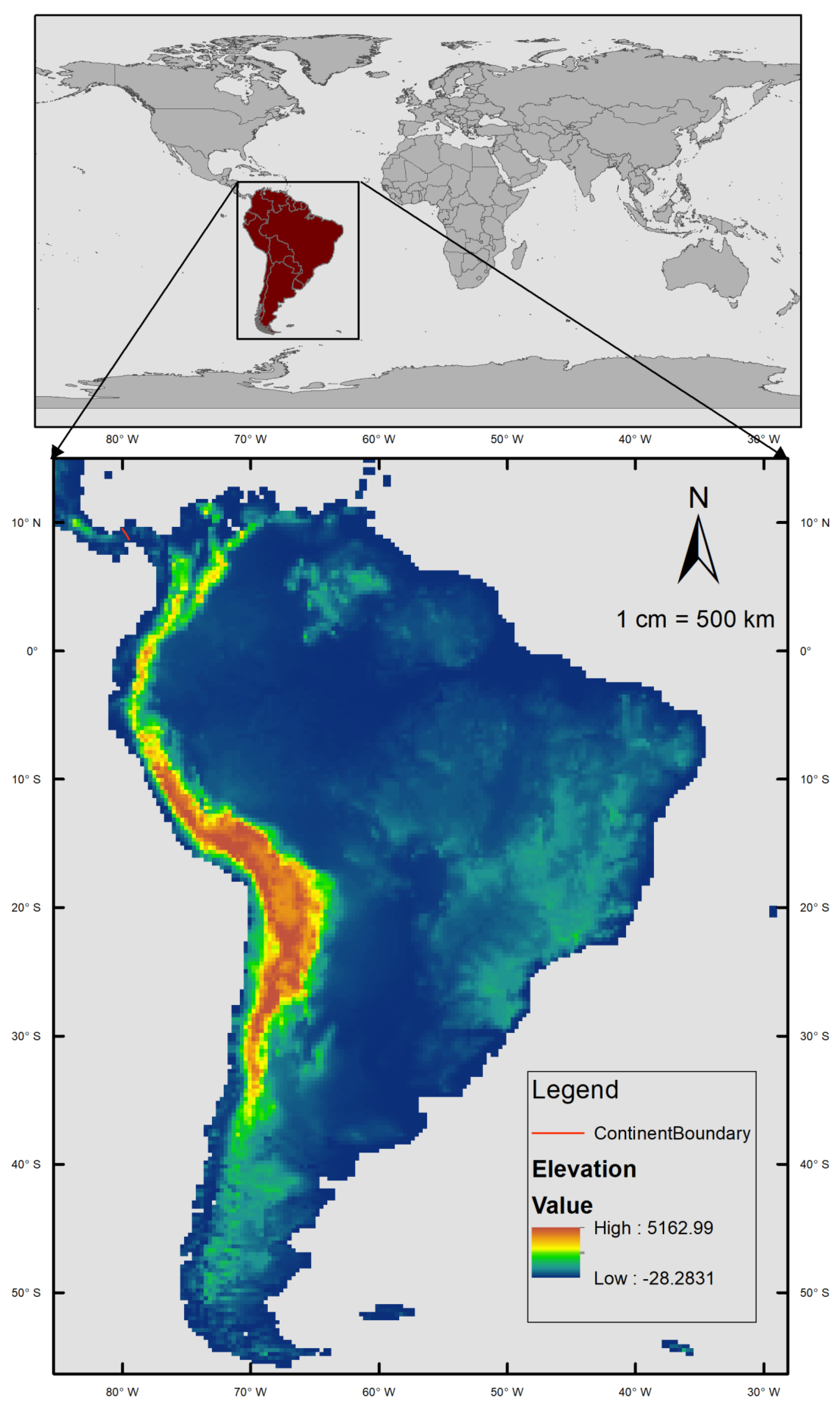
Figure 1. Geographical location and elevation map of the study area.
Remotesensing 13 03643 g001
Figure 2. A framework for actual evapotranspiration assessment and projection based on meteorological, hydrological, and vegetation remote sensing products.
Remotesensing 13 03643 g002
Figure 3. Intra-(a) and interannual (b) variations of AET in South America.
Remotesensing 13 03643 g003
Figure 4. Spatial distribution of multi-year average AET (a) and MK statistic Z (b).
Remotesensing 13 03643 g004
Figure 5. Spatial distribution map of average AET in four seasons. (a) Mar-May, (b) Jun-Aug, (c) Sep-Nov, (d) Dec-Feb.
Remotesensing 13 03643 g005
Figure 6. Spatial distribution map of MK statistic Z in four seasons. (a) Mar-May, (b) Jun-Aug, (c) Sep-Nov, (d) Dec-Feb.
Remotesensing 13 03643 g006
Figure 7. Map of P-coefficients between monthly AET and each factor. (a) T, (b) P, (c) PET, (d) NDVI, (e) R, (f) TWC.
Remotesensing 13 03643 g007
Figure 8. Map of determinants for AET at each order from Boruta. (a) First, (b) Second, (c) Third, (d) Fourth, (e) Fifth, and (f) Sixth.
Remotesensing 13 03643 g008aRemotesensing 13 03643 g008b
Figure 9. Distribution of the simulation accuracy R 2 of two models under different input strategies.
Remotesensing 13 03643 g009
Figure 10. The joint optimal prediction of two models under different input strategies.
Remotesensing 13 03643 g010
Figure 11. The map of historical multi-year average value from CRU and the prediction value in 2030 from CMIP6 about T, P and PET.
Remotesensing 13 03643 g011
Table 1. Summary of the dataset applied in this study.
VariablesAbbr.VersionSpatial
Resolutions
Time SpanData Source (11 July 2021)
TemperatureTCRU TS Version 4.050.5 degrees2001–2020https://crudata.uea.ac.uk/cru/data/hrg/cru_ts_4.05/ge/
PrecipitationPCRU TS Version 4.050.5 degrees2001–2020https://crudata.uea.ac.uk/cru/data/hrg/cru_ts_4.05/ge/
Potential
evapotranspiration
PETCRU TS Version 4.050.5 degrees2001–2020https://crudata.uea.ac.uk/cru/data/hrg/cru_ts_4.05/ge/
Actual
evapotranspiration
AETGLDAS Noah2.10.25 degrees2000–2020https://disc.gsfc.nasa.gov/datasets/
Surface runoffQsGLDAS Noah2.10.25 degrees2000–2020https://disc.gsfc.nasa.gov/datasets/
Subface runoffQsbGLDAS Noah2.10.25 degrees2000–2020https://disc.gsfc.nasa.gov/datasets/
Snowmelt runoffQsmGLDAS Noah2.10.25 degrees2000–2020https://disc.gsfc.nasa.gov/datasets/
Total water storage changesTWCJPL GRACE(-FO) RL060.5 degrees2002–2020https://grace.jpl.nasa.gov/
Normalized
Difference
Vegetation Index
NDVIMOD13C2
Version6
0.05 degrees2000–2020https://lpdaac.usgs.gov/products/mod13c2v006/
TemperatureTCMIP6-NCAR
SSP245
100 km2020–2090https://esgf-node.llnl.gov/projects/cmip6/
PrecipitationPCMIP6-NCAR
SSP245
100 km2020–2090https://esgf-node.llnl.gov/projects/cmip6/
Potential
evapotranspiration
PETIPSL-CM6A-LR
SSP245
250 km2020–2090https://cmc.ipsl.fr/all-projects/
Table 2. The statistic value of Z from the MK test and the climate change rate from linear trend regression.
MonthZ-ValueClimate Change Rate (mm/10a)
January3.155.59
February3.435.31
March2.384.52
April3.154.97
May2.875.61
June2.594.78
July2.033.28
August1.682.72
September0.280.62
October0.770.15
November1.752.61
December2.033.23
Table 3. Assessment of the P-correlation and determinant order of monthly average AET in South America.
TPPETNDVIRTWC
Correlation
coefficient
0.8320.8130.5870.8220.2670.638
Boruta-order of importanceFirstThirdFourthSecondSixthFifth
Table 4. The proportion of the area that is controlled by each factor in the whole of South America at each order (%).
OrderTPPETNDVIRTWC
First10.34 13.97 23.22 24.85 21.52 6.10
Second20.02 15.41 21.39 16.61 22.46 4.13
Third14.69 16.59 21.34 21.49 21.27 4.63
Fourth12.46 26.98 18.35 13.23 21.22 7.75
Fifth25.73 17.94 14.25 11.04 12.50 18.53
Sixth16.76 9.11 1.45 12.78 1.04 58.86
Table 5. Three projection input strategies of AET.
Input StrategiesMeteorological
Factors
Vegetation IndexHydrological
Factors
Description
Input
S1
T, P, and PET
From CMIP6
Not inputNot inputOnly Forced by the meteorological
Factors during 2020–2090
Input
S2
T, P, and PET
From CMIP6
Monthly historical average NDVINot inputThe future monthly NDVI roughly represented by the historical mean value
Input
S3
T, P, and PET
From CMIP6
Monthly historical average NDVIMonthly historical average R and TWCThe future monthly NDVI, R, and TWC roughly represented by the historical mean value
Table 6. The proportion of the grids that the R 2 exceeds the following value in the whole of South American (%).
Input StrategiesModel
R 2   >   0.9
R 2   >   0.7
R 2   >   0.5
Input
S1
RF4.7342.0959.17
SVR2.5228.6745.43
Input
S2
RF16.9551.6164.84
SVR9.2642.8554.95
Input
S3
RF16.5753.9470.70
SVR10.2742.7955.70
Publisher’s Note: MDPI stays neutral with regard to jurisdictional claims in published maps and institutional affiliations.