Optimal Grid-Based Filtering for Crop Phenology Estimation with Sentinel-1 SAR Data

Abstract

In the last decade, suboptimal Bayesian filtering (BF) techniques, such as Extended Kalman Filtering (EKF) and Particle Filtering (PF), have led to great interest for crop phenology monitoring with Synthetic Aperture Radar (SAR) data. In this study, a novel approach, based on the Grid-Based Filter (GBF), is proposed to estimate crop phenology. Here, phenological scales, which consist of a finite number of discrete stages, represent the one-dimensional state space, and hence GBF provides the optimal phenology estimates. Accordingly, contrarily to literature studies based on EKF and PF, no constraints are imposed on the models and the statistical distributions involved. The prediction model is defined by the transition matrix, while Kernel Density Estimation (KDE) is employed to define the observation model. The approach is applied on dense time series of dual-polarization Sentinel-1 (S1) SAR images, collected in four different years, to estimate the BBCH stages of rice crops. Results show that 0.94 ≤ R² ≤ 0.98, 5.37 ≤ RMSE ≤ 7.9 and 20 ≤ MAE ≤ 33.

1. Introduction

Knowing the current status of crops is essential for effective agricultural management, whose aim is to maximize crop production and, at the same time, to reduce the impact of agriculture on the environment [1].

Within such a framework, timely information on crop phenological stages, provided at both regional and national scale, supports national and international institutions (e.g., including insurance companies, advisory organizations, etc.) in scheduling yield calendars and assessing yield losses, managing claims subsidies, and so on. As an example, the flood events that affected Bangladesh in 2017 [2] caused severe damages to the agricultural sector, especially to rice cultivation. In this case, the knowledge of rice phenology at the time of the floods was primarily important to assess the impact on rice production. Regarding the floods in March–April, official authorities estimated severe damages to almost 220,000 hectares of boro rice, whose growing stages were identified as “ready-to-be harvested” [2]. Finally, crop phenology serves as an input for agronomic models, e.g., for comprehending the water and energy exchanges between the cultivated land and the atmosphere [3].

Remote sensing represents an effective tool to monitor agricultural crops [1], since it allows continuous observations of wide agricultural areas. In particular, microwave remote sensing provide day and night and almost all-weather observations.

Within such a framework, spaceborne Synthetic Aperture Radar (SAR) sensors, able to provide observations at fine spatial resolution, are well suited for crop monitoring [4]. In addition, the use of polarimetric SAR (PolSAR) systems allows an enhanced sensitivity to the physical and structural characteristics of the plants, which change along the cultivation cycle. Clearly, a key requirement for this application is the availability of time series of data with short revisit time.

With this respect, the Sentinel-1 (S1) satellites, as a part of the Copernicus program of the European Commission, are greatly contributing to agricultural monitoring, including crop-type mapping [5], phenology estimation [6] and the monitoring of crop biophysical parameters [7]. The S1 fleet consists of two polar-orbiting satellites, S1A and S1B, which mount on board C-band SAR instruments with dual-polarimetric capabilities, i.e., HH+HV or VH+VV channels (where H and V stand for horizontal and vertical polarization, respectively), and operating in different imaging modes [8]. The Interferometric Wide Swath (IW) mode provides images with a swath width of 250 km at a moderate spatial resolution (5 × 20 m). Both S1A and S1B have a revisit time of 12 days, which is reduced to 6 days when the two satellites are combined. As a matter of fact, the Sentinel sensors and the associated data policy constitute an unprecedented source of data to build operational monitoring services in the agricultural domain [9], due to the free and open access to the data and the availability of dense time series.

In this study, S1 data are exploited for real time estimation of phenological stages of agricultural crops. In the last decade, several approaches [6,10,11,12,13,14,15,16,17,18,19,20,21,22,23] have been proposed to estimate crop phenology with SAR data. The approaches in [10,11,12,13,14,15,16,17,18] apply classification methods (based on hierarchical trees, decision planes, the Wishart statistics and machine learning algorithms) on the PolSAR features to classify phenological intervals. Here, the classified phenology at the current date is based only on the current image, without accounting for the temporal evolution of the crops. On the other hand, the methods in [6,19,20,21,22,23] are based on the dynamical systems theory. In this case, suboptimal Bayesian Filtering (BF) techniques, i.e., Extended Kalman Filtering (EKF) and Particle Filtering (PF), are used to combine the crop evolution with the current PolSAR acquisition, in order to provide a filtered estimate of the current phenological stage. Such a dynamic framework was first introduced in [19], where EKF is employed to estimate rice phenology, based on the use of X-band TerraSAR-X (TSX) PolSAR data. EKF is also used in [20], where the approach is applied to C-band RADARSAT-2 (RS2) data to estimate phenological stages of other cereal crops. Regarding PF, it was first exploited in [21], to estimate both phenological stages and agricultural dates (i.e., sowing and panicle initiation dates) of rice fields. Note that, also in such works, the estimated phenology consists of phenological intervals, i.e., a discrete variable is estimated. The studies in [6,22] use PF to estimate rice phenology on a continuous scale. In [6], authors introduce a dynamic threshold algorithm for S1 data to estimate the rice transplanting dates, and a hierarchical tree to initialize the PF algorithm. In [22], PF is applied on a time series of TSX and Normalized Difference Vegetation Index (NDVI), including air temperature data. In such works, since phenology is considered to be a continuous variable, both the prediction model (which describes the phenology evolution with time) and the observation model (which relates the PolSAR features to the phenology) are defined with curve fitting. In [23], PF is applied to estimate canola phenology with RS2 data. Here, the PF approach provides estimates of the crop maturity, a continuous variable which is directly related to discrete phenological stages. It is important to remark that such BF algorithms can be, in general, applied to other remote sensing data, including optical (e.g., see study in [24]), and also in a data fusion context, to combine different remotely sensed data (as demonstrated in [22]). In summary, among all the BF methods, EKF and PF have been exploited so far for crop phenology estimation.

In this study, a novel approach, based on an optimal BF algorithm, the Grid Based Filter (GBF), is proposed to estimate crop phenology with dual-polarization S1 SAR data. Here, crop phenology is regarded as a discrete and finite variable. Accordingly, the GBF filter presents a number of advantages compared with EKF and PF algorithms (see Section 2 namely: (i) no constraints, such as linearization, curve fitting or Gaussian assumptions, are imposed on the prediction and observation model; and (ii) the algorithm provides the optimal estimation of crop phenology, in contrast with EKF and PF that do not satisfy the optimality criterion.

2. Methodology

The proposed approach is described in this section, where the method is formulated for generic SAR observations. Hence, it can be straightforwardly applied to data collected by any kind of SAR configuration and/or other remote sensing sensors.

Throughout the paper, the following notation is adopted: unless otherwise specified, a stochastic variable is denoted with roman type, while its realizations are denoted in italic.

2.1. Background

Agricultural crops can be regarded as dynamical systems [20]. Within this framework, the crop variables at discrete time t_k (which include phenology, crop height, etc.) are referred to as state variables, and collected into a vector, the state vector x_k, whose domain is known as state space [25].

Since this study is focused on the estimation of only one state variable, phenology, hereinafter a one-dimensional system is considered to describe its evolution with time. We will explore the inter-relations between the state variables, i.e., considering a multi-dimensional state vector, in future studies.

Such a one-dimensional system is shown in (1) [26], where $\mathrm{x}\left(t_k\right)$, i.e., the phenological stage at time $t_k$, is denoted with ${\mathrm{x}}_k$. $f(·)$ is the prediction model [22], and it is a function, generally non-linear, of the state at time $t_{k-1}$, ${\mathrm{x}}_{k-1}$, with ${\mathrm{v}}_{k-1}$ being the system noise.

$${\mathrm{x}}_k=f({\mathrm{x}}_{k-1},{\mathrm{v}}_{k-1})$$

(1)

The SAR features measured at time $t_k$ are related to the state ${\mathrm{x}}_k$ according to (2) [26].

$${\mathbf{y}}_k=\mathit{h}({\mathrm{x}}_k,{\mathbf{e}}_k)$$

(2)

Here, ${\mathbf{y}}_k$ is the observation vector at time $t_k$, which collects the SAR features relevant to the monitored crop at that time. $\mathit{h}(·)$ is the observation model [22], a vector-valued function, generally non-linear, of ${\mathrm{x}}_k$, with ${\mathbf{e}}_k$ being the observation noise. Note that the vector nature of $\mathit{h}(·)$ and ${\mathbf{e}}_k$ is due to the dimension of ${\mathbf{y}}_k$, denoted with $N_y$. Furthermore, note that the functions $f(·)$ and $\mathit{h}(·)$ are time-invariant here, since they depend on the state ${\mathrm{x}}_k$, and not on the time index k.

The filtered estimate of the current state ${\mathrm{x}}_k$ is based on all the available measurements up to time $t_k$, i.e., ${\mathit{y}}_{1:k}=\{{\mathit{y}}_1,\dots ,{\mathit{y}}_k\}$ [26]. Within this framework, BF techniques are aimed at reconstructing the posterior probability density function (pdf) $p\left({\mathrm{x}}_k\right|{\mathit{y}}_{1:k})$ [26]. In particular, by assuming that (i) the initial states distribution $p\left({\mathrm{x}}_0\right|{\mathit{y}}_0)=p\left({\mathrm{x}}_0\right)$ is known (no observation is provided at time $t_0$), and that (ii) the state ${\mathrm{x}}_k$ in (1) follows a first-order Markov process, $p\left({\mathrm{x}}_k\right|{\mathit{y}}_{1:k-1}{y}_{1:k})$ can be obtained recursively in two steps: prediction and update. At time $t_{k-1}$, the prediction step uses the prediction model (1) to obtain the prior pdf of ${\mathrm{x}}_k$, $p\left({\mathrm{x}}_k\right|{\mathit{y}}_{1:k-1})$. Then, at time $t_k$, when the measurement is available, the update step consists of updating the prior by using the observation model, thus providing the posterior pdf $p\left({\mathrm{x}}_k\right|{\mathit{y}}_{1:k})$. The latter can be referred to as the complete solution to the estimation problem [26] since it statistically characterizes ${\mathrm{x}}_k$. This solution is, generally, analytically intractable, and it exists in two restrictive cases: the Kalman filter (KF) and the GBF, which are referred to as optimal BF methods [26]. KF assumes Gaussian distributions for both ${\mathrm{v}}_{k-1}$ and ${\mathbf{e}}_k$, and that the functions $f(·)$ and $\mathit{h}(·)$ are linear. In the case of GBF, the only requirement is that the state space is discrete and with finite dimensions. Moreover, no statistical assumptions are made, where ${\mathrm{v}}_{k-1}$ and ${\mathbf{e}}_k$ follow an arbitrary distribution, and no constraints are imposed on $f(·)$ and $\mathit{h}(·)$.

When the Gaussian and linearity assumptions do not hold, and when the state space is not discrete and finite, neither KF nor GBF can be used, and $p\left({\mathrm{x}}_k\right|{\mathit{y}}_{1:k})$ can be approximated by suboptimal algorithms. The latter include EKF and PF [26]. EKF employs a local linearization when $f(·)$ and $\mathit{h}(·)$ are not linear, approximating the noise distributions with Gaussian pdfs. Regarding PF, it belongs to the family of the Sequential Monte Carlo (SMC) methods, where the posterior pdf is represented by random samples (termed “particles”) with associated weights. PF approaches do not impose any constraints neither on the ${\mathrm{v}}_{k-1}$ and ${\mathbf{e}}_k$ pdf, nor on $f(·)$ and $\mathit{h}(·)$, and hence they are particularly suited for dynamical estimation of continuous variables. For this reason, PF began a great interest in crop phenology estimation with SAR data (see Section 1). In this case, the phenology is either regarded as a continuous variable or, like in [23], it is related to another continuous variable. Accordingly, the functions $f(·)$ and $\mathit{h}(·)$ are obtained by curve fitting [6,22]. Regarding $f(·)$, the temporal evolution of phenology (provided by ground data) is analyzed while, in the case of $\mathit{h}(·)$, the behavior of the SAR observables is evaluated as a function of phenology. Finally, fitting approaches (e.g., based on polynomials ) are used to define these functions. Moreover, Gaussian distributions are invoked for both ${\mathrm{v}}_{k-1}$ and ${\mathbf{e}}_k$ to facilitate the modeling.

A different approach is proposed in this study, where the optimal GBF is exploited for crop phenology estimation. Our modeling strategy is to consider the phenological evolution of crops as a discrete and finite state space. This is possible since, although crop phenology is a continuous state variable, it is commonly measured by means of numerical scales, where specific growth stages are labeled with discrete codes. For instance, in the case of the BBCH scale (from Biologische Bundesanstalt, Bundessortenamt und CHemische Industrie) [27], the one-dimensional state space of rice comprises 58 states labeled from 0 to 99. Due to the reduced number of states, the dynamic system can be modeled as a first-order Markov process through the transition matrix formalism. This approach provides several advantages with respect to EKF and PF:

1.

Neither modeling $f(·)$ and $\mathit{h}(·)$, nor making assumptions on the noise distributions is required.

2.

Considering phenology as a discrete and finite state variable, the proposed GBF approach is the only method to provide optimal phenology estimates. In contrast, when dealing with continuous variables, EKF and PF are approximate nonlinear BF that provide suboptimal estimates [26].

3.

The transition matrix is a widely used formulation in many fields (robotics, speech recognition, bioinformatics, etc.). This general framework is simpler to implement than EKF and PF algorithms. In addition, it is straightforward to train the prediction model in real time by updating the transition probabilities.

In summary,

Table 1. Filter comparison according the model restrictions and optimality in phenological estimation.

Filter	Prediction/Observation Model	Noise Model	Optimality
KF	Linear equation	Gaussian	Optimal
EKF	Linearization	Gaussian	Sub-optimal
PF	Curve fitting	No restriction	Sub-optimal
Grid-based filter	No restriction	No restriction	Optimal

shows a comparison of such BF approaches in terms of model restrictions and optimality.

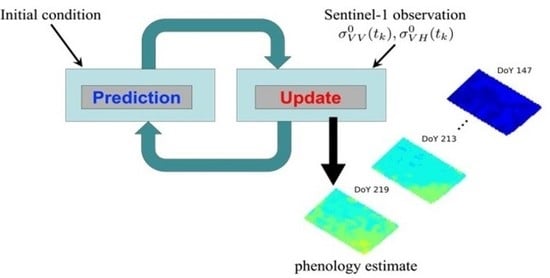
2.2. Grid-Based Filter for SAR-Based Phenology Estimation

GBF provides the optimal solution to the dynamical estimation problem, if the state space is discrete and finite [26]. In this case, the functions $f(·)$ and $\mathit{h}(·)$, as well as the statistical characterization of ${\mathrm{v}}_{k-1}$ and ${\mathbf{e}}_k$, can be arbitrary.

Crop phenology is commonly measured by means of numerical scales, e.g., [27], which consist of discrete values ranging in a defined interval. In this study, such discrete stages are regarded as the state variable to estimate. Therefore, we use GBF to provide an optimal solution for phenology estimation, based on the use of SAR measurements.

Let us consider an agricultural test site where SAR acquisitions are available every n days. Hence, the observation vector measured at a given time (2) consists of those SAR features (e.g., backscattering coefficients) which are selected for the estimation. Then, let us consider a discrete phenological scale, referred to as $\mathcal{S}=\{x^i,i=1,\dots ,N_s\}$, where $x^i$ and $N_s$ are the ith phenological stage and the total number of stages, respectively. For a given initial distribution $p\left({\mathrm{x}}_0\right)$, the GBF reconstructs the posterior pdf of such states in a recursive way, providing a phenology estimate as soon as a new SAR observation is available. For the purpose of this study, we assume that the sowing date of the fields is known, and hence we consider only those SAR acquisitions collected after sowing. We will extend the approach to provide the estimation of the sowing date in a future study.

Without loss of generality, we can express the posterior pdf at time $t_{k-1}$ as shown in (3) [26], where $\delta (·)$ is the Dirac Delta, and the weights $w_{k-1|k-1}^i=\mathrm{Pr}\{{\mathrm{x}}_{k-1}=x^i|{\mathit{y}}_{1:k-1}\}$, $i=1,\cdots ,N_s$, represent the conditional probabilities of the state at time ${\mathrm{x}}_{k-1}$, given the SAR features measured until $t_{k-1}$.

$$p\left({\mathrm{x}}_{k-1}\right|{\mathit{y}}_{1:k-1})=\sum _{i=1}^{N_s}{w}_{k-1|k-1}^i\delta ({\mathrm{x}}_{k-1}-x^i)$$

(3)

The prediction step allows predicting the distribution of the states at time $t_k=t_{k-1}+n$, resulting in the prior pdf, shown in (4) [26]. Here, the weights are based on the observations up to time $t_{k-1}$, as shown in (5).

$$p\left({\mathrm{x}}_k\right|{\mathit{y}}_{1:k-1})=\sum _{i=1}^{N_s}{w}_{k|k-1}^i\delta ({\mathrm{x}}_k-x^i),$$

(4)

$$w_{k|k-1}^i=\sum _{j=1}^{N_s}{w}_{k-1|k-1}^{j}p\left({\mathrm{x}}_k^i\right|{\mathrm{x}}_{k-1}^j),i=1,\cdots ,N_s$$

(5)

As we previously introduced, the states (1) follow a first-order Markov process. Therefore, the conditional pdf $p\left({\mathrm{x}}_k\right|{\mathrm{x}}_{k-1})$ describes the transitions of phenological stages between two successive time steps. Furthermore, note that in (3)–(5) all the possible states are considered, that is, the entire set $\mathcal{S}$ represents the state space at each time step. Generally, this is not the case for crop phenology, where the set of possible states is expected to change with time as crops evolve. Accordingly, the state space at time $t_k$, say ${\mathcal{S}}_k$, is a subset of $\mathcal{S}$, and it is dictated by the crop evolution. The states in ${\mathcal{S}}_k$ naturally fulfill two constraints: (1) phenological stages are chronologically ordered, i.e., ${\mathrm{x}}_k\ge {\mathrm{x}}_{k-1}$; (2) no sharp variations are expected between consecutive stages over a short period of time, such as in the case of a $n=6$ days revisit time. These two conditions imply that, at each time step, among all the states in $\mathcal{S}$, only a small set of states, i.e., the ones in ${\mathcal{S}}_k$, must have non-zero weights (5). The remaining states represent unrealistic stages, and they have to be excluded. This is done in two steps. First, ${\mathcal{S}}_k$ is determined as it will be explained in Section 2.3.3. Then, once the weights for all the possible states in $\mathcal{S}$ are obtained from (5), unrealistic stages are excluded as shown in (6), with the resulting weights being normalized.

$$\begin{array}{c}{w}_{k|k-1}^i=0,\forall x_i\notin {\mathcal{S}}_k\\ \downarrow \\ w_{k|k-1}^i=\frac{w_{k|k-1}^i}{{\sum }_{i=1}^{N_s}{w}_{k|k-1}^i},i=1,\cdots ,N_s\end{array}$$

(6)

At time $t_k$, a new SAR observation is available, and hence a new vector, ${\mathit{y}}_k$, is measured. Then, at the update step the weights are updated as shown in (7) [26].

$$w_{k|k}^i=\frac{\mathcal{L}\left(x^i\right|{\mathit{y}}_k)w_{k|k-1}^i}{{\sum }_{i=1}^{N_s}\mathcal{L}\left(x^i\right|{\mathit{y}}_k)w_{k|k-1}^i},i=1,\cdots ,N_s$$

(7)

In this case, $\mathcal{L}\left(x^i\right|{\mathit{y}}_k)$ represents the likelihood function, which is obtained from the statistical characterization of ${\mathbf{y}}_k$ (2) evaluated at ${\mathit{y}}_k$. Finally, the posterior pdf is shown in (8).

$$p\left({\mathrm{x}}_k\right|{\mathit{y}}_{1:k})=\sum _{i=1}^{N_s}{w}_{k|k}^i\delta ({\mathrm{x}}_k-x^i)$$

(8)

In this study, we consider the mode of such a discrete density as an estimate of phenology at time $t_k$, as shown in (9).

$${\widehat{\mathrm{x}}}_k=\underset{x^i}{argmax}\left(w_{k|k}^i\right)$$

(9)

2.3. GBF Modeling

To apply the proposed approach, the GBF parameters must be defined: the initial pdf $p\left({\mathrm{x}}_0\right)$, the prediction and the observation model, and the state space ${\mathcal{S}}_k$.

The theoretical rationale underpinning these parameters is described in this section. Regarding the generation of the models, this is undertaken before the implementation of the method, using data relevant to training fields. In particular, the initial pdf of the states, the prediction model, and ${\mathcal{S}}_k$ are defined using only ground data on phenological stages provided for these fields. Then, to define the observation model, SAR data, collected over training fields during the growing season, are used along with ground data.

2.3.1. Initial Distribution

In this study, a uniform distribution over the interval [$x_{0_{low}},x_{0_{upp}}$] is selected as initial density $p\left({\mathrm{x}}_0\right)$. The lower bound, $x_{0_{low}}$ is chosen as the initial value of the scale $\mathcal{S}$. Then, $x_{0_{upp}}$ is obtained using training fields, and it corresponds to the maximum phenological stage observed n days after sowing.

2.3.2. Prediction Model

Since the states (1) represent a first-order Markov process, we adopt the transition matrix formalism [28] to characterize their transitions in two consecutive time steps.

For a given phenological scale $\mathcal{S}$, we consider the one-day transition matrix ${\mathbf{P}}^{t_k,t_k+1}$, i.e.; the $N_s\times N_s$ matrix shown in (10). Here, the entry $p_{ji}=\mathrm{Pr}\{\mathrm{x}(t_k+1)=x^i|\mathrm{x}\left(t_k\right)=x^j\}$ represents the one-day transition probability which characterizes the transition from state $x^j$ at day $t_k$ to state $x^i$ at day $t_k+1$.

$${\mathbf{P}}^{t_k,t_k+1}=\left[\begin{array}{ccccc}{p}_{11}& p_{12}& \cdots & p_{1N_s-1}& p_{1N_s}\\ 0& p_{22}& \cdots & p_{2N_s-1}& p_{2N_s}\\ ⋮& ⋮& \ddots & ⋮& ⋮\\ 0& 0& \cdots & p_{N_s-1N_s-1}& p_{N_s-1N_s}\\ 0& 0& \cdots & 0& p_{N_s{N}_s}\end{array}\right]$$

(10)

Note that (10) ensures that phenological stages are chronologically ordered, with $p_{ij}=0$, $\forall x_i,x_j\in \mathcal{S}$. Furthermore, note that the transition probabilities do not depend on time, according to the assumption that $f(·)$ (1) is time-invariant. Therefore, such probabilities are said to be stationary [28] and, hereinafter, ${\mathbf{P}}^{t_k,t_k+1}$ is referred to as $\mathbf{P}$. Accordingly, the n-days transition matrix ${\mathbf{P}}^{t_k,t_k+n}$, which characterizes the states transitions over n days, is shown in (11) [28].

$${\mathbf{P}}^{t_k,t_k+n}=\underset{n\mathrm{times}}{\underbrace{\mathbf{P}·\mathbf{P}···\mathbf{P}}}={\mathbf{P}}^n$$

(11)

We can now express the prediction Equation (5) as shown in (12), where ${\mathit{w}}_{k-1|k-1}=[w_{k-1|k-1}^1,\cdots ,w_{k-1|k-1}^{N_s}]$ collects the actual weights at day $t_{k-1}$, while ${\mathit{w}}_{k|k-1}=[w_{k|k-1}^1,\cdots ,w_{k|k-1}^{N_s}]$ collects the predicted weights for day $t_k$.

$${\mathit{w}}_{k|k-1}={\mathit{w}}_{k-1|k-1}{\mathbf{P}}^n$$

(12)

Therefore, defining the prediction model consists of determining the transition matrix $\mathbf{P}$. This is undertaken using training data where, for each phenological stage, the one-day transitions are evaluated. As a consequence, we do not need neither modeling the function $f(·)$, nor making assumptions on the ${\mathrm{v}}_{k-1}$ distribution.

It is important to note that since $\mathbf{P}$ collects the one-day transition probabilities, the revisit time n is not necessarily fixed, but it can vary with time. This is particularly advantageous in a data fusion context where, for instance, SAR observations are combined with optical data. In such a scenario n is the revisit time of the combined time series, and it varies according to the cloud conditions that severally affect optical measurements.

2.3.3. State Space ${\mathcal{S}}_k$

Regarding ${\mathcal{S}}_k$, it represents the set of possible phenological stages at time $t_k$, and its knowledge allows excluding unrealistic stages (6).

${\mathcal{S}}_k$ is determined from the transition matrix ${\mathbf{P}}^n$ (11). In fact, given that the phenology estimate at time $t_{k-1}$ is ${\widehat{\mathrm{x}}}_{k-1}=x^j$, the jth row of this matrix, ${\mathbf{P}}_{j*}^n$, is considered to obtain ${\mathcal{S}}_k$. ${\mathbf{P}}_{j*}^n$ collects the transition probabilities which characterize the state ${\mathrm{x}}_k$, as shown in (13), where $p_{ji}^n=\mathrm{Pr}\{{\mathrm{x}}_k=x^i|{\mathrm{x}}_{k-1}=x^j\}$.

$${\mathbf{P}}_{j*}^n=[p_{j1}^n,\cdots ,p_{j{N}_s}^n]$$

(13)

The set ${\mathcal{S}}_k$ consists of those stages associated with non-zero probabilities, as shown in (14). Such a set is bounded between $x_{k_{low}}$ and $x_{k_{upp}}$, with $x_{k_{low}}\ge {\widehat{\mathrm{x}}}_{k-1}$.

$${\mathcal{S}}_k=\{x_i\in \mathcal{S}:p_{ji}^n>0\}=\{x_{k_{low}},\cdots ,x_{k_{upp}}\}$$

(14)

2.3.4. Observation Model

Defining the observation model consists of providing the statistical characterization of the $N_y$–dimensional vector ${\mathbf{y}}_k$ (2). This is undertaken using training fields and considering the observation vector measured for these fields at each phenological stage. However, in this study, rather than modeling the function $\mathit{h}(·)$ with curve fitting and assuming a certain distribution for ${\mathbf{e}}_k$, Kernel Density Estimation (KDE) [29] is employed to model the pdf of ${\mathbf{y}}_k$.

Let us consider a set of training parcels being at stage $x^i$. The observation vector relevant to such parcels is referred to as ${\mathbf{y}}_{tr}^i$. The KDE estimate of the pdf of ${\mathbf{y}}_{tr}^i$ conditioned to $x^i$, $p\left({\mathbf{y}}_{tr}^i\right|x^i)$, is shown in (15) [29].

$$\widehat{p}\left({\mathbf{y}}_{tr}^i\right|x^i)=\sum _{j=1}^{N_{tr}}{K}_H({\mathbf{y}}^i-{\mathit{y}}_j^i),i=1,\cdots ,N_s$$

(15)

The vectors $\{{\mathit{y}}_1^i,\cdots ,{\mathit{y}}_{N_{tr}}^i\}$ are the $N_{tr}$ samples measured at the training parcels locations. $K_H\left(\mathbf{u}\right)={\left|\mathit{B}\right|}^{-1}{K\left(\right|\mathit{B}|}^{-1}\mathbf{u})$ is the scaled multivariate kernel, with $K(·)$ being the multivariate kernel function, and $\mathit{B}$ the $N_y\times N_y$ bandwith matrix [29]. KDE (15) is undertaken for each discrete stage of the scale $\mathcal{S}$, resulting in $N_s$ pdfs. These distributions are used to model the pdf of ${\mathbf{y}}_k$ at each stage of the phenological scale, i.e., $p\left({\mathbf{y}}_k\right|x^i)=\widehat{p}\left({\mathbf{y}}_{tr}^i\right|x^i),i=1,\cdots ,N_s$.

Finally, during the estimation, when the vector ${\mathit{y}}_k$ is measured, $p\left({\mathbf{y}}_k\right|x^i)$ allows obtaining the likelihood function $\mathcal{L}\left(x^i\right|{\mathit{y}}_k)$, as shown in (16).

$$\mathcal{L}\left(x^i\right|{\mathit{y}}_k)=p({\mathbf{y}}_k={\mathit{y}}_k|x^i),i=1,\cdots ,N_s.$$

(16)

3. Test Site and Data Sets

The proposed approach is here applied to estimate phenological stages of rice fields using S1 SAR data.

The test site consists of an area of 30 km × 30 km close to the mouth of the Guadalquivir river, Sevilla, SW of Spain (37.1N, 6.15W), where rice is cultivated annually from May to October, approximately. A Google Earth picture of the test site is shown in Figure 1.

General rice species in this area is Oryza sativa L. The specific variety cultivated in the monitored fields corresponds to a long grain type named puntal, quite common in Spain and other similar temperate regions.

In this specific location, sowing is carried out by spreading seeds randomly from an airplane over the fields, which are already flooded at that time. Then, farming practices in this area ensure the presence of a water layer on the ground during the whole cultivation period. Exceptionally, for 3–4 days at the first month of the campaign the fields are emptied to carry out fumigation, and then they are flooded again. The cultivation campaign lasts about 135–150 days in this location.

3.1. Ground Campaign Data

Since 2009, the local association of rice farmers (Federacion de Arroceros de Sevilla) has collected every year (except in 2012) detailed ground measurements on a weekly basis for a set of 4–7 selected parcels spread over the site. Note that the polygons of these parcels are overlaid, with different colors, on the Google Earth picture in Figure 1.

The weekly measurements include phenological stages according to the BBCH scale [27], which is described in detail in Section 3.1.1. These data are provided at the parcel level, i.e., a single BBCH value identifies the phenology of the whole parcel. However, for years 2013–2020 the minimum and the maximum BBCH stages detected in each parcel are also provided.

Along with phenology records, the following information is also known for each parcel: total area (ha), sowing date, harvest date, and final yield (kg/ha). Particular aspects for some of them have been registered also, such as fertilization activities, water salinity, and presence of diseases. Note that neither sowing nor harvest are simultaneous in all parcels of the site, being around 3 to 4 weeks the time span between the first and the last of the monitored parcels in both activities. The number of monitored parcels each year, and the corresponding number of phenology reference data, are detailed in

Table 2. Ground reference data: parcels and measurements per year. This dataset is subdivided into testing and training data (see Section 4.1).

Year	Number of Parcels	Ground Measurements
2009	6	115
2010	7	151
2011	6	114
2013	6	131
2014	6	135
2015	4	77
2016	7	142
2017	7	134
2018	7	141
2019	5	101
2020	6	121
Total	67	1362

. Note that for the implementation of the method, these data are subdivided into training and testing data, as it will be detailed in Section 4.1. Training data are used for the generation of the prediction model, and as an input to define the observation model. Regarding testing data, these are employed to evaluate the accuracy of the final phenology estimates. Finally, there is also climate information provided by the Spanish Government under the Sistema de Informacion Agroclimatica para el Regadio (SIAR), including daily files of temperature, precipitation, humidity, and wind. In this region, a rainy season is common at the beginning of autumn every year.

3.1.1. BBCH Scale of Rice

The BBCH scale of rice is depicted in

Table 3. BBCH scale used to describe rice phenology. Green: vegetative phase. Orange: reproductive phase. Brown: maturation phase.

Principal Growth Stage	Secondary Growth Stages (BBCH Codes)
0: Germination	00, 01, 03, 05, 06, 07, 09
1: Leaf development	10–19
2: Tillering	21–29
3: Stem elongation	30, 32, 34, 37, 39
4: Booting	41, 43, 45, 47, 49
5: Inflorescence emergence, heading	51–59
6: Flowering, anthesis	61, 65, 69
7: Development of fruit	71, 73, 75, 77
8: Ripening	83, 85, 87, 89
9: Senescence	92, 97, 99

. Such a scale consists of ten principal growth stages, from Germination to Senescence (see left column of Table 3). Each of these principal stages is subdivided into secondary growth stages (whose name is not listed for sake of space), labeled with a code that ranges from 0 to 99 (right column of Table 3). The secondary stages represent the final BBCH stages, with the corresponding codes being the final BBCH values. Usually, a certain BBCH stage of the parcel is identified if at least the $50\%$ of the plants in the parcel reaches that stage [27]. This aspect is considered in Section 5.1, where ground data are compared with the estimated stages to assess the performance accuracy. We will see that, at some points in the growing cycle, parcels develop heterogeneously, and this influences the accuracy analysis.

From Table 3 we note that the number of secondary stages is not the same among the principal stages. For instance, while the principal stage “Tillering” consists of 9 secondary stages (from BBCH 21 to BBCH 29), “Flowering” comprises only three stages, i.e., BBCH 61, 65, and 69. Hence, the numerical interval between two consecutive BBCH codes is, in general, non-uniform, thus resulting in a discrete numerical scale with a total of 58 stages, where the first and the last stages are assigned to BBCH 0 and BBCH 99, respectively. Finally, three main phases characterize the rice evolution: the vegetative phase (BBCH 0–49, highlighted in green); the reproductive phase (BBCH 51–69, highlighted in orange); the maturation phase (from BBCH 71–49, highlighted in brown).

3.2. Sentinel-1 Data and Processing

In this study, we employ all the available images of one orbit acquired by the S1A/B constellation from 2017 to 2020, hence ensuring a revisit time of 6 days and allowing for 4 different annual campaigns. Dual-polarization VV-VH images in Ground Range Detected (GRD) format, corresponding to orbit number 74 (ascending pass), are used, which are always acquired at 18:15 approximately.

The processing of the series of images is carried out with the SNAP software provided by ESA, and consists of the following steps:

1.

Apply orbit files.

2.

Thermal noise removal.

3.

Subset to the area of interest.

4.

Radiometric calibration to backscattering coefficient (${\sigma }^0$).

5.

Speckle filter: IDAN with window size equal to 20.

6.

Conversion from linear to dB.

7.

Orthorectification (step named Terrain Correction in SNAP) to a cartographic grid with pixel size equal to 10 m.

As a last step, a stack is formed in SNAP with all the images of each year to ensure a pixel-by-pixel correspondence of all the images. For the analysis at parcel level, all the pixels located inside the polygons defined for each parcel and year are extracted.

4. Experiments

In this section, we present the experiments undertaken on the S1 dataset. We first describe the testing/training data and the GBF modeling and then show the results for phenology estimation.

4.1. Testing and Training Data

In this study, we undertake four experiments, one for each year of S1 acquisitions, from 2017 to 2020. When the S1 data from a given year are selected to be tested, they are not included in the filter modeling. The corresponding year is referred to as the testing year, and the ground data from that year are used to evaluate the final phenology estimates. The remaining years are referred to as training years, and they are used to define the GBF models.

Table 4. List of testing and training years for each experiment undertaken.

Experiment No.	Testing Year	Training Years for the Prediction Model (Available Ground Data)	Training Years for the Observation Model (Available S1 Data)
1	2020	2009–2019	2017, 2018, 2019
2	2019	2009–2018, 2020	2017, 2018, 2020
3	2018	2009–2017, 2019, 2020	2017, 2019, 2020
4	2017	2009–2016, 2018–2020	2018, 2019, 2020

lists, for each testing year, the corresponding training years to be used for the prediction and observation model.

4.2. GBF Modeling

The entire set $\mathcal{S}$ consists of the BBCH scale. In this study, we consider BBCH 1 (“Beginning of seed imbibition” [27]) as the initial stage of the cycle (sowing). Therefore, $\mathcal{S}=\{1,\cdots ,99\}$, with a total number of stages $N_s$ = 58.

4.2.1. Initial Distribution

In this case, the lower bound for the initial distribution is ${\mathrm{BBCH}}_{0_{low}}=1$. Then, having a 6-day revisit time, the upper bound ${\mathrm{BBCH}}_{0_{upp}}$ consists, for each set of training years, of the maximum BBCH code, observed among all the parcels, at 6-days after sowing.

4.2.2. Prediction Model and State Space ${\mathcal{S}}_k$

The one-day transition matrix $\mathbf{P}$ (10) relevant to the BBCH scale is a $58\times 58$ matrix. For a given testing year, the transition matrix to be used is defined by considering the BBCH stages relevant to the parcels monitored in the corresponding training years (third column of Table 4). In particular, $\mathbf{P}$ is obtained with the following steps:

1.

Interpolation. For each parcel of each training year, since ground data are provided on a weekly basis, we assume local linearity between phenology and time. Accordingly, the measured BBCH stages are linearly interpolated to obtain values on a one-day basis.

2.

Discretization. The interpolated values are discretized to obtain values belonging to the BBCH scale (see Table 3).

3.

Computation of the one-day transition probabilities. The discretized BBCH stages are used to compute the probability of transiting from stage $BBC{H}^j$ to stage $BBC{H}^i$ in one day, $p_{ji}$. For a given stage $BBC{H}^j$, the total number of parcels transiting to $BBC{H}^i$ among all the training years is considered. Then, $p^{ji}$ is given by (17).

$$p^{ji}=\frac{totalnumberoftransitionsfromstageBBC{H}^{j}tostageBBC{H}^{i}inoneday}{totalnumberoftransitionsfromstageBBC{H}^{j}inoneday}$$

(17)

In this study, since the S1 data have a revisit time $n=6$ days, we use (11) to compute the 6-day step transition matrix ${\mathbf{P}}^6$.

In order to illustrate the prediction model, we use the transition matrix obtained from the training years 2009–2019 (see Table 4). Here, we consider two cases, assuming two different estimates at time $t_{k-1}$. In the first (second) case, we assume that ${\widehat{\mathrm{BBCH}}}_{k-1}=1$ (${\widehat{\mathrm{BBCH}}}_{k-1}=53$). Then, Figure 2a,b show the transition probabilities (13) conditioned to ${\mathrm{BBCH}}^j=1$ and ${\mathrm{BBCH}}^j=53$, respectively. Note that, in both cases, ${\mathcal{S}}_k$, i.e., the set of possible stages at time $t_k$, is also annotated. This is determined using (14), and results in ${\mathcal{S}}_k=\{1,\cdots ,13\}$ and ${\mathcal{S}}_k=\{53,\cdots ,73\}$, for the first and the second case, respectively.

4.2.3. Observation Model

For a given monitored field, the observation vector at time $t_k$ is ${\mathbf{y}}_k=[{\Sigma }_{VV}^0\left(t_k\right),{\Sigma }_{VH}^0\left(t_k\right)]$, with ${\Sigma }_{VV}^0\left(t_k\right)$ and ${\Sigma }_{VH}^0\left(t_k\right)$ denoting the stochastic variable associated with the received VV and VH backscattering coefficient, respectively. For each testing year, the pdf of ${\mathbf{y}}_k$ at each BBCH stage is modeled by the joint pdf of the backscattering coefficients estimated from the data in the corresponding training years (last column of Table 4). In particular, for a given set of training years, the following steps are undertaken:

1.

Interpolation. For each parcel of each training year, the measured BBCH stages are linearly interpolated to obtain the BBCH codes at the radar acquisition dates.

2.

Discretization. The interpolated values are discretized to obtain values belonging to the BBCH scale.

3.

Stacking. For each polarimetric channel, the ${\sigma }^0$ values of all the pixels extracted from the parcels polygons of all the training years are stacked according to the discretized stages. These stacked values are the training samples of the backscattered powers at each stage of the BBCH scale.

4.

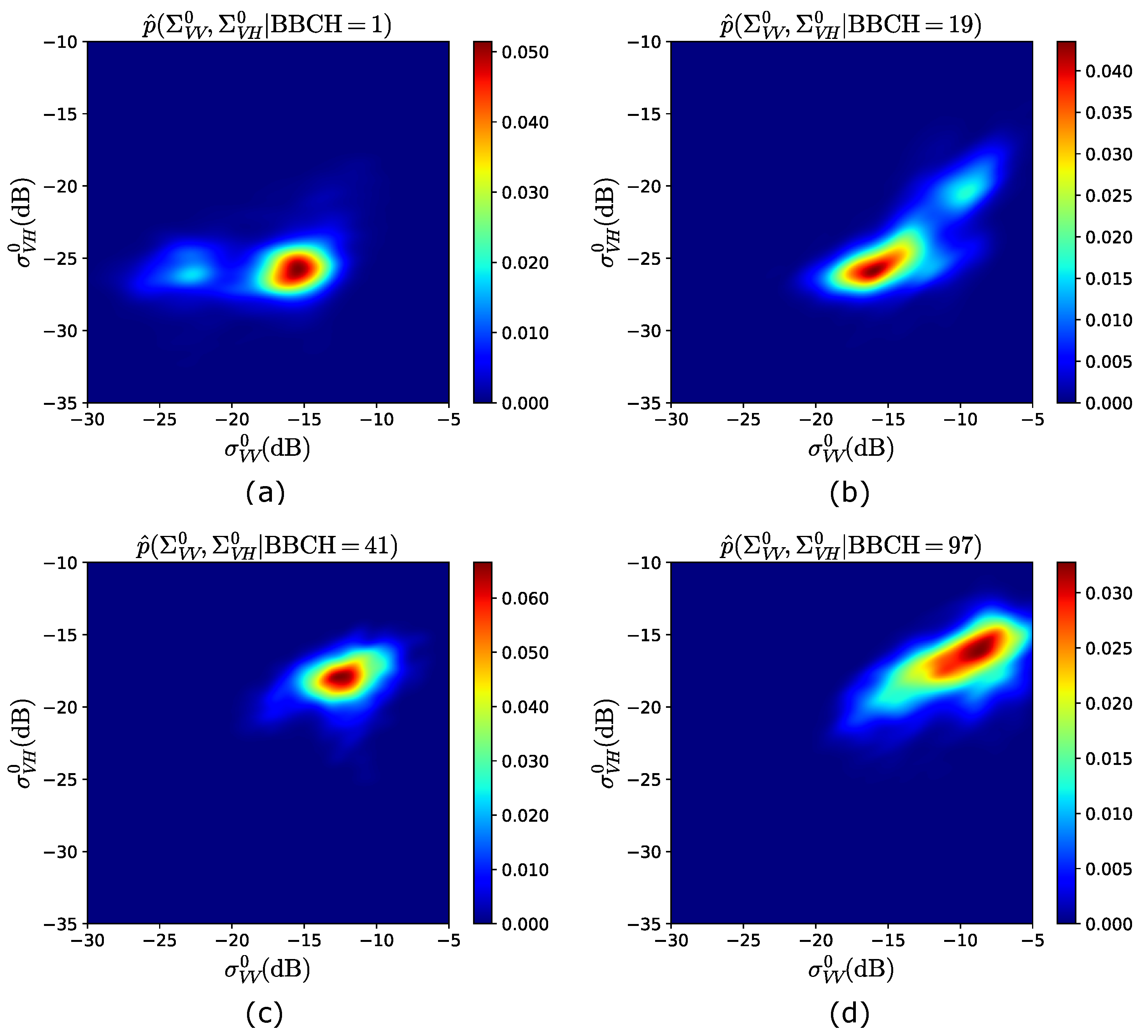
KDE. For each BBCH stage, KDE (15) is applied to these samples to estimate the joint pdf of ${\Sigma }_{VV}^0$ and ${\Sigma }_{VH}^0$, using the multivariate Gaussian kernel [29] to model $K(·)$. This results in $N_s=58$ estimated pdfs, i.e.; $\widehat{p}({\Sigma }_{VV}^0,{\Sigma }_{VH}^0|\mathrm{BBCH}={\mathrm{BBCH}}^i)$, $i=1,2,\cdots ,58$. This set of distributions consists of the observation model to be used when the GBF is implemented on the testing data.

Figure 3 shows a 2D view of the pdfs estimated from the training years 2017–2019, at $\mathrm{BBCH}=1$, 19, 47 and 97. At BBCH = 1 (see Figure 3a), as expected, the backscattered powers are mainly distributed around ${\sigma }_{VV}^0\approx -15$ dB and ${\sigma }_{VH}^0\approx -26$ dB, with a second (lower) peak of the pdf at ${\sigma }_{VV}^0\approx -24$ dB (${\sigma }_{VH}^0\approx -26$ dB). Then, at $\mathrm{BBCH}=19$, i.e., end of “Leaf development” (see Table 3), although the highest pdf’s peak is approximately unchanged, the distribution is spread over larger backscattering values, as shown in Figure 3b. In fact, ${\Sigma }_{VV}^0$ (${\Sigma }_{VH}^0$) is mainly distributed between ∼$-20$ and ∼$-8$ dB (∼$-28$ and ∼$-18$ dB), resulting in a second peak centered at ${\sigma }_{VV}^0\approx -9$ dB and ${\sigma }_{VH}^0\approx -20$ dB. This is caused by the fact that leaves are developed and plants are approaching tillering, i.e., more plants elements are present, for which the received powers start to increase. Hence, in Figure 3c, at BBCH = 41 (first stage of “Booting”, see Table 3), while ${\Sigma }_{VH}^0$ results in values mainly larger than ∼$-20$ dB, ${\Sigma }_{VV}^0$ is distributed between ∼$-15$ and ∼$-9$ dB, as a consequence of the extinction phenomena [12] caused by the vertical stems, which induces an attenuation on the vertically polarized waves. Finally, an overall increase of the backscattered powers is observed at the end of the season (BBCH = 97) in Figure 3d, with the peak of the pdf being around ${\sigma }_{VV}^0\approx -8$ dB and ${\sigma }_{VH}^0\approx -16$ dB.

The likelihood function is obtained from the observation model using (16). However, contrarily to approaches based on curve fitting, which result in a smooth likelihood, here $\mathcal{L}\left({\mathrm{BBCH}}^i\right|{\mathit{y}}_k)$, $i=1,\cdots ,N_s=58$, is noisier, due to the fact that large backscattering variations are observed over 58 stages only. Therefore, during the estimation, 1D KDE with Gaussian kernels is performed to smooth $\mathcal{L}(·)$.

4.3. GBF Implementation

Figure 4 depicts the implementation of GBF to estimate the BBCH stages of rice using S1 images. Note that, for a given field, only the S1 acquisitions collected after sowing are considered.

When the first image is available, at time $t_1$, the observation vector ${\mathit{y}}_1=[{\sigma }_{VV}^0\left(t_1\right),{\sigma }_{VH}^0\left(t_1\right)]$ is provided. In this case, the prior pdf $p\left({\mathrm{BBCH}}_1\right|{\mathit{y}}_0)$ is the initial distribution $p\left({\mathrm{BBCH}}_0\right)$. Regarding the likelihood function $\mathcal{L}\left({\mathrm{BBCH}}^i\right|{\mathit{y}}_1)$, it is first obtained from the observation model using (16), and then smoothed with KDE. Then, since $p\left({\mathrm{BBCH}}_0\right)$ is uniform over the interval [${\mathrm{BBCH}}_{0_{low}}$, ${\mathrm{BBCH}}_{0_{upp}}$], the weights $w_{0|0}^i$ (7) consist of the normalized likelihood evaluated in that interval. Therefore, the first estimate ${\widehat{\mathrm{BBCH}}}_1$ only depends on the likelihood.

Successively, the filter recursively estimates the BBCH stages as soon as a new S1 image is available.

Once that the $k-1$th estimation is provided, both ${\widehat{\mathrm{BBCH}}}_{k-1}$ and the vector ${\mathit{w}}_{k-1|k-1}$ serve as inputs for the prediction step. Here, the prediction model $\mathbf{P}$ is used to define the 6-day transition matrix ${\mathbf{P}}^6$ (11). Then, once the weights at $t_k$ are predicted (12), the jth ${\mathbf{P}}^6$ row (13) corresponding to ${\widehat{\mathrm{BBCH}}}_{k-1}$ is used to determine ${\mathcal{S}}_k$ (14). Successively, unrealistic stages are excluded and the weights normalized (6).

At time $t_k$, a new S1 acquisition results in the vector ${\mathit{y}}_k=[{\sigma }_{VV}^0\left(t_k\right),{\sigma }_{VH}^0\left(t_k\right)]$. This, along with the observation model $p\left({\mathbf{y}}_k\right|{\mathrm{BBCH}}^i)$, is used as an input at the update step to obtain the likelihood $\mathcal{L}\left({\mathrm{BBCH}}^i\right|{\mathit{y}}_k)$ (16). The latter is first smoothed with KDE, and then, by applying (7), is used to update the weights obtained at the prediction step. Finally, the resulting weights $w_{k|k}^i$, which in turn yield the posterior pdf $p\left({\mathrm{BBCH}}_k\right|{\mathit{y}}_{1:k})$ (8), allow obtaining the kth BBCH estimate (9), ${\widehat{\mathrm{BBCH}}}_k$.

4.4. Estimation Results

For each of the four testing years, the proposed approach is applied to every pixel of each monitored parcel. Regarding the interval over which the initial distribution is defined, in all the cases the upper bound derived from the training data is ${\mathrm{BBCH}}_{0_{upp}}=11$. Hence, a uniform distribution in the interval BBCH 1–11 is selected as the initial distribution for all the experiments.

For a given testing year, the estimation is validated by comparing the retrieved BBCH stages with the true ones, measured during the ground campaign in that year. The true phenological stages at the S1 acquisition dates are obtained by linear interpolation (and then discretization) of the ones provided by ground data. Since the latter are provided at the parcel level, the validation is also undertaken at the parcel level. That is, for a given parcel, at a given acquisition date, the mode of the estimated phenology of all the pixels is considered as the final BBCH estimate for the parcel. Then, the estimated parcel phenology at all the acquisitions is compared with the true one by evaluating the Root Mean Squared Error (RMSE), the coefficient of determination ($R^2$), and the Maximum Absolute Error (MAE).

Figure 5a–d show the estimation performance, considering all the testing parcels, for the four years 2017–2020. Note that the RMSE, $R^2$ and MAE values are annotated in the figure. Furthermore, note that, for year 2017 (years 2019 and 2020) the parcel which results in the best (worst) accuracy is annotated in red and with a different mark.

A very good agreement is observed between the estimated and the true BBCH stages. As a matter of fact, for the four testing years RMSE $\le 8$, $R^2\ge 0.94$, and a maximum MAE of 33 are observed.

The best performance is obtained for the year 2017, which shows RMSE $\approx 5.4$, $R^2=0.98$ and MAE = 20. In such a case, the best estimation is achieved for parcel El Reboso, highlighted with red star marks. Hereinafter, this parcel is referred to as BEST. Then, while for the year 2018 we observe RMSE $\approx 6.7$, $R^2=0.95$ and MAE = 24, the estimations in the years 2019 and 2020 perform worst, with RMSE $\approx 8$, $R^2=0.94$ and MAE = 33 (RMSE $\approx 7.5$, $R^2=0.94$ and MAE = 24) for 2019 (2020). Note that, for each of these two years, the performances are degraded by an “outlier”, which corresponds to parcel Puebla (hereinafter referred to as O1) and El Reboso (hereinafter referred to as O2) in 2019 and 2020, respectively. These outliers, along with parcel BEST, are analyzed in the next section.

Finally, Figure 5e shows the performance achieved by combining the four testing years. RMSE is ∼6.8, while $R^2$ and MAE are 0.95 and 33, respectively. This is a key result, considering that both the prediction and the observation model are defined by the statistical distributions of the training data, without neither employing curve fitting strategies, nor assuming a particular statistical distributions.

5. Discussion

5.1. Analysis of the Estimation Performance

In this section, the performances of the estimations are discussed and carefully analyzed.

Regarding the accuracy values, these are around the ones obtained by the PF approach applied on S1 VH products in [6], where the authors state that $R^2=0.96$ and RMSE = 5.82 are achieved when the transplanting dates are estimated correctly.

Regarding the estimation performances in specific phenological intervals, all the experiments result in very good estimations of BBCH in the range 1–40 (see Figure 5). Then, a larger dispersion of the estimates is observed approximately in the range 40–80. Such a dispersion, which is almost negligible for the year 2017 and quite evident for the remaining years, is primarily due to two causes. First, phenology is estimated recursively. This implies that, if at time $t_k$ an anomalous stage is estimated, then the corresponding posterior distribution is likely to affect the estimates at successive epochs. Second, the attenuation due to extinction experienced at the stem elongation/booting stages of rice [12] might also result in large estimation errors. In fact, this attenuation, more pronounced at the VV channel, vanishes at later stages, thus leading to an increase of the backscattered powers. This results in a multimodal likelihood function which, depending on the set ${\mathcal{S}}_k$, might affect the final estimation. Moreover, the extinction phenomena are proportional to the plant density of the parcels. Therefore, if a parcel is too dense (sparse) the attenuation is more (less) significant, and this affects the likelihood which, in turn, might result in underestimations (overestimations).

It is important to underline that the evaluation of performances depends on the heterogeneous development of the parcels, and the sampling protocols used by practitioners to measure the BBCH stages during the ground campaign. As explained in Section 3.1.1, the BBCH stage of a parcel is assigned when at least the half of plants of the parcel has reached that stage. Such a criterion does not account for the within parcel variability, i.e., different areas of a parcel might develop at different rates. If this variability is present in certain phases of the season and, more importantly, if it is also detected by the GBF estimates, then the parcel level analysis is not enough for a comprehensive performances assessment. In fact, when such heterogeneity is not considered, the performance evaluated in a specified range (such as BBCH 40–80) might not be totally realistic. In the following, we consider the minimum and maximum BBCH values provided by ground data for the testing parcels in the years 2017–2020 to assess the heterogeneous development of the parcels, especially in the range BBCH 40–80. Such minimum and maximum values are used as a reference to analyze the GBF pixel estimates of the parcels. If these estimates lie between these two extreme reference values, then their variability is in accordance with the real parcel heterogeneity, and the estimation performances in the range BBCH 40–80 might be, in reality, better than the ones evaluated by the parcel level analysis. Otherwise, if a large discrepancy is observed, the parcel level analysis provides a comprehensive evaluation. Figure 6 shows, for each testing year, the pixel estimates of the parcels versus the Day of The Year (DoY). Note that since the GBF estimates consist of discrete values, at a given acquisition date, different pixels estimated as being in the same BBCH stage are located at the same point in the plot. Therefore, we set a level of color transparency to represent the estimated values, such that light colors (i.e., light gray) indicate a lower amount of estimates at that stage, while dark colors (i.e., black) represent a high number of points. In each plot, the shadow area highlighted in cyan represents the area delimited by the minimum and maximum BBCH reference values, obtained from all the parcels in the corresponding year. The ground data reference area indicates a heterogeneous development in all the years. This variability is less significant at the early stages, while is more pronounced at BBCH 40–80. Regarding the pixel estimates, they mainly lie in the ground reference area for all the years but the year 2020. This indicates that for years 2017–2019, the estimated variability is in agreement with the heterogeneous development of the parcels. Hence the parcel level analysis evaluation is not comprehensive in this case. A different situation is observed for the year 2020, where a significant amount of pixel estimates lies outside the shadow area from DoY 250 to DoY 300. This denotes that the results in Figure 5d provide a comprehensive evaluation of the observed underestimations.

We now turn to analyze the estimation for parcels BEST, O1, and O2, relevant to the years 2017, 2019, and 2020, respectively. Regarding parcel BEST, when considered alone, it results in outstanding accuracies, with RMSE $\approx 3.76$, $R^2\approx 0.99$ and MAE = 10. On the contrary, parcel O1 (O2) is significantly overestimated (underestimated) at stages BBCH 40–80, resulting in $RMSE\approx 14.4$, $R^2\approx 0.9$ and MAE = 33 (RMSE ≈ 12.2, $R^2\approx 0.89$ and MAE = 24).

In order to provide further insights on these results, we show examples of phenology estimates. For such a purpose, we considered, for each of the three parcels, those pixels which provided the final estimates (i.e., the mode) shown in Figure 5. The average ${\sigma }_{VV}^0$ and ${\sigma }_{VH}^0$ values evaluated over these pixels are considered, and the approach is applied to such values to obtain parcel-level estimates. The performances are almost identical to the ones obtained at the pixel-basis shown in Figure 5, with some slight differences, as expected. The parcel-level estimations at some acquisition dates are shown, for each parcel, in Figure 7. Here, the weights $w_{k|k-1}^i$ and $w_{k|k}^i$ (highlighted with blue and black vertical stems, respectively), along with the likelihood function (highlighted in red), are plotted against the BBCH stages. The true BBCH (${\mathrm{BBCH}}_{true}$), along with the estimated one, is annotated in the plots.

Regarding parcel BEST (see Figure 7a), since this is very well estimated at all the dates, only one phenology estimate is considered, i.e., the one at the 15th acquisition (DoY 231), where $BBC{H}_{true}=51$. In this case, ${\mathcal{S}}_k=\{51,\cdots ,73\}$, and the weights $w_{k|k-1}^i$ exhibit a peak at $\mathrm{BBCH}=61$, which represent the predicted stage. Then, in the interval ${\mathcal{S}}_k$ the likelihood sharply increases from $\sim {10}^{-3}$ to $\sim 0.07$, thus resulting in the weights $w_{k|k}^i$ being maximum at $BBCH=55$, which is the final estimate. This example clearly shows how the stage predicted by $w_{k|k-1}^i$ is improved by the S1 observation through the likelihood.

In the case of parcel O1 (see Figure 7b,c), we consider two estimates, at $t_{10}$ and $t_{20}$, corresponding to DoY 185 (${\mathrm{BBCH}}_{true}$= 25) and DoY 245 (${\mathrm{BBCH}}_{true}$= 54), respectively. At DoY 185, ${\mathcal{S}}_k=\{29,\cdots ,43\}$, with the weights $w_{k|k-1}^i$ (the likelihood) being maximum at $\mathrm{BBCH}=32$ ($\mathrm{BBCH}=25$). Then, the resulting weights $w_{k|k}^i$ provide $\widehat{\mathrm{BBCH}}=29$. Note that, also in this case, the predicted stage ($\mathrm{BBCH}=32$) is worse than the final estimation. A completely different situation is observed at DoY 245. Here, ${\mathcal{S}}_k=\{69,\cdots ,89\}$, and the weights $w_{k|k-1}^i$ have their maximum at $\mathrm{BBCH}=83$. Note that the set ${\mathcal{S}}_k$ does not include the stage ${\mathrm{BBCH}}_{true}$. This is due to the recursive nature of the filter, for which the overestimations experienced at the previous acquisitions (see Figure 5c, where the true BBCH ranges from stage 40 to 61) results in ${\mathcal{S}}_k$ being different than the expected one. Then, a multimodal likelihood, with four relative maxima at BBCH 28, 55, 73 and 85, is observed. This is explained by the fact that the backscattered powers (not shown to save space) exhibit similar values at these stages. At ${\mathrm{BBCH}}_{true}$ such powers are higher than expected, thus causing two peaks in the likelihood over the set ${\mathcal{S}}_k$, at BBCH 73 and 85. This is due to one of the following reasons: the parcel is less dense than parcel BEST (as stated by ground information) and hence the attenuation due to extinction is less significant; the variability observed in the parcel development at this date is too large, as shown in Figure 6c. Finally, once that the predicted weights are updated by the likelihood, the final estimate is $\widehat{\mathrm{BBCH}}=83$.

Regarding parcel O2 (see Figure 7d,e), also in this case two estimations are considered, at DoY 174 (${\mathrm{BBCH}}_{true}=11$) and DoY 234 (${\mathrm{BBCH}}_{true}=56$). In the first case, ${\mathcal{S}}_k=\{11,\cdots ,21\}$, and the weights $w_{k|k-1}^i$ exhibit the maximum value at BBCH = 21. The likelihood is maximum at BBCH = 11, resulting in $w_{k|k}^i$ being maximum at $\mathrm{BBCH}=12$, which represents the final estimate. Again, in this case, the prediction is improved by the likelihood. Then, on DoY 234, ${\mathcal{S}}_k=\{34,\cdots ,49\}$, with the weights $w_{k|k-1}^i$ being maximum at $\mathrm{BBCH}=37$. Regarding the likelihood, it is again multimodal, with two larger peaks at $\mathrm{BBCH}=29$ and $\mathrm{BBCH}=54$. Between these two stages, the likelihood is approximately flat, for which the updated weights $w_{k|k}^i$ are almost identical to the predicted ones. This result in an underestimation, with $\widehat{\mathrm{BBCH}}=37$. Note that such a worse performance is not driven by the within parcel variability, as discussed above, but is caused by the recursive nature of GBF. In fact, stage BBCH 54, which corresponds to the maximum likelihood, is not included in ${\mathcal{S}}_k$. Hence, as a result of the underestimations experienced at the previous acquisitions (visible in Figure 5d, at BBCH 40 to 61), ${\mathcal{S}}_k$ results in a set of significantly lower stages, thus affecting the current estimation.

5.2. Illustration of Pixel-Level Phenology Estimates

To provide a visual inspection of the heterogeneous crop development, Figure 8 shows the pixel-level phenology estimates, at each S1 acquisition date, for the parcel BEST. Note that the DoY corresponding to the radar acquisition dates is also annotated. From ground data, we know that the parcel is sown on DoY 145 (May 25) and harvested on DoY 289 (October 16).

On the first acquisition, at DoY 147, most of the pixels are estimated at BBCH 6, while for the remaining ones, BBCH 10–11 is observed. Then, the parcel approaches smoothly BBCH 11–13 on DoY 159, although a few pixels result in later stages (BBCH 21). On DoY 165, although the parcel phenology is mainly in BBCH 21, some areas are still in BBCH 12–13. Then, up to DoY 183, the estimated phenology smoothly transits from BBCH 21 to BBCH 23. On DoY 189 the parcel is mainly at BBCH 29, with some inner heterogeneous zones at BBCH 23–24. Successively, from DoY 195 to DoY 213 the parcel is mainly in the "Stem elongation" stage, with the estimated BBCH ranging from 32 to 37 (see Table 3) for the majority of the pixels. However, at these dates a large within field variability is observed. In particular, at DoYs 195–201 two inner zones, which include approximately those heterogeneous pixels observed at DoY 189, develop slower than the surrounding ones. This situation changes at DoYs 207–213, where, in most of the cases, a smooth transition from BBCH 34 to BBCH 37 is observed. Moreover, we note that, from DoY 201 toward the end of the season, an area corresponding to the lower corner of the parcel develops faster than the rest. For instance, this area is mainly at BBCH 51 at DoY 213, when the rest of the field is at BBCH 37. The same behavior is observed at DoY 237, when this zone is at BBCH 77, while the remaining pixels are mainly at BBCH 58–61. Such a different development rate is less evident starting from DoY 261, when this lower corner and the remaining areas are at BBCH 89 and BBCH 87, respectively. Finally, the field develops up to the last phenological stages, to be mainly at BBCH 99 at DoY 285.

In conclusion, the heterogeneous development of crop phenology plays a key role in the proposed GBF estimation approach. The within fields variability of the GBF estimates (in agreement with field data) is significant at stages BBCH 40–80. This has an important impact, since this BBCH interval is one of the most relevant for decision support purposes on the cultivation (spraying, fertilization, or impact of weather conditions, etc.).

On the other hand, the recursive nature of the filter, and the ambiguous backscattering behavior of the crops in certain phenological stages might result in significant under- and over-estimations. Future studies will be devoted to improving such estimation errors. For instance, this could be addressed by extending the approach to real time estimation of the sowing date, which would allow optimizing the evolution of the state space, or considering other variables, such as temperature data (e.g., like in [22] with PF), as “driving forces” of the phenological evolution.

Last but not least, data fusion approaches, e.g., combining SAR with optical observations, can be easily accommodated in our method. This will also be considered in future research steps. As a matter of fact, the transition matrix after $n_C$ days, with $n_C$ being the variable revisit time of the SAR/optical time series, is straightforwardly obtained from the model.

6. Conclusions

In this study, a novel approach, based on the use of GBF, is proposed for real time crop phenology estimation with SAR data. Here, any phenological scale which consists of a finite number of discrete stages is regarded as a one-dimensional state space. In this context, GBF provides the optimal phenology estimates.

The method is applied on dense time series of dual-pol VV-VH S1 SAR images, collected in the years 2017–2020, to estimate the BBCH stages of rice. For each testing year, GBF is implemented, taking as inputs the models defined with data in the corresponding training years.

The results obtained confirm the soundness of the proposed approach, which yields $0.94\le R^2\le 0.98$, $5.37\le \mathrm{RMSE}\le 7.9$ and $20\le$ MAE $\le 33$. Moreover, the analysis on the estimations performances in different years shows that:

• When rice fields are at stages BBCH 1–40, on average, the final estimation, provided by the S1 observation through the likelihood (update step), outperforms the prediction.
• For years 2017–2019, the within fields variability detected by GBF, more pronounced at stages BBCH 40–80, is in agreement with the heterogeneous development present in ground data.
• Due to the recursive nature of the filter, worse estimates at a given time could severally affect the estimations at successive time epochs. This is especially true at approximately BBCH 40–80, where the extinction phenomena caused by the elongating vertical stems might affect the likelihood function and then result in large estimation errors.

References

1. Atzberger, C. Advances in Remote Sensing of Agriculture: Context Description, Existing Operational Monitoring Systems and Major Information Needs. Remote Sens. 2013, 5, 949–981. [Google Scholar] [CrossRef] [Green Version]
2. FAO. GIEWS Update-Bangladesh. GIEWS. 2017. Available online: https://www.fao.org/3/i7876e/i7876e.pdf (accessed on 21 October 2021).
3. Liu, F.; Chen, Y.; Shi, W.; Zhang, S.; Tao, F.; Ge, Q. Influences of agricultural phenology dynamic on land surface biophysical process and climate feedback. J. Geogr. Sci. 2017, 27, 1085–1099. [Google Scholar] [CrossRef]
4. Steele-Dunne, S.C.; McNairn, H.; Monsivais-Huertero, A.; Judge, J.; Liu, P.; Papathanassiou, K. Radar Remote Sensing of Agricultural Canopies: A Review. IEEE J. Sel. Topics Appl. Earth. Observ. Remote Sens. 2017, 10, 2249–2272. [Google Scholar] [CrossRef] [Green Version]
5. Mestre-Quereda, A.; Lopez-Sanchez, J.M.; Vicente-Guijalba, F.; Jacob, A.W.; Engdahl, M.E. Time-Series of Sentinel-1 Interferometric Coherence and Backscatter for Crop-Type Mapping. IEEE J. Sel. Topics Appl. Earth Observ. Remote Sens. 2020, 13, 4070–4084. [Google Scholar] [CrossRef]
6. Yang, H.; Pan, B.; Li, N.; Wang, W.; Zhang, J.; Zhang, X. A systematic method for spatio-temporal phenology estimation of paddy rice using time series Sentinel-1 images. Remote Sens. Environ. 2021, 259. [Google Scholar] [CrossRef]
7. Mandal, D.; Kumar, V.; Ratha, D.; Dey, S.; Bhattacharya, A.; Lopez-Sanchez, J.M.; McNairn, H.; Rao, Y.S. Dual polarimetric radar vegetation index for crop growth monitoring using Sentinel-1 SAR data. Remote Sens. Environ. 2020, 247, 2020. [Google Scholar] [CrossRef]
8. European Space Agency. Sentinel-1 User Handbook; European Space Agency: Paris, France, 2013. [Google Scholar]
9. Joint Research Center. Concept Note: Towards Future Copernicus Service Components in Support to Agriculture? Available online: https://www.copernicus.eu/sites/default/files/2018-10/AGRI_Conceptnote.pdf (accessed on 15 September 2021).
10. Lopez-Sanchez, J.M.; Cloude, S.R.; Ballester-Berman, J.D. Rice phenology monitoring by means of SAR polarimetry at X-band. IEEE Trans. Geosci. Remote Sens. 2012, 50, 2695–2709. [Google Scholar] [CrossRef]
11. Lopez-Sanchez, J.M.; Vicente-Guijalba, F.; Ballester-Berman, J.D.; Cloude, S.R. Estimating phenology of agricultural crops from space. In ESA Living Planet Symp.; European Space Agency: Edinburgh, UK, 2013; ESA-SP 722. [Google Scholar]
12. Lopez-Sanchez, J.M.; Vicente-Guijalba, F.; Ballester-Berman, J.D.; Cloude, S.R. Polarimetric response of rice fields at C-band: Analysis and phenology retrieval. IEEE Trans. Geosci. Remote Sens. 2014, 52, 2977–2993. [Google Scholar] [CrossRef] [Green Version]
13. Yang, Z.; Li, K.; Liu, L.; Shao, Y.; Brisco, B.; Li, W. Rice growth monitoring using simulated compact polarimetric C band SAR. Radio Sci. 2014, 49, 1300–1315. [Google Scholar] [CrossRef]
14. Mascolo, L.; Lopez-Sanchez, J.M.; Vicente-Guijalba, F.; Mazzarella, G.; Nunziata, F.; Migliaccio, M. Retrieval of phenological stages of onion fields during the first year of growth by means of C-band polarimetric SAR measurements. Int. J. Remote Sens. 2015, 36, 3077–3096. [Google Scholar] [CrossRef] [Green Version]
15. Yuzugullu, O.; Erten, E.; Hajnsek, I. Rice growth monitoring by means of X-band co-polar SAR: Feature clustering and BBCH scale. IEEE Geosci. Remote Sens. Lett. 2015, 12, 1218–1222. [Google Scholar] [CrossRef]
16. Lopez-Sanchez, J.M.; Vicente-Guijalba, F.; Ballester-Berman, J.D.; Cloude, S.R. Influence of incidence angle on the coherent copolar polarimetric response of rice at X-band. IEEE Geosci. Remote Sens. Lett. 2015, 12, 249–253. [Google Scholar] [CrossRef] [Green Version]
17. Mascolo, L.; Lopez-Sanchez, J.M.; Vicente-Guijalba, F.; Nunziata, F.; Migliaccio, M.; Mazzarella, G. A complete procedure for crop phenology estimation with PolSAR data based on the complex Wishart classifier. IEEE Trans. Geosci. Remote Sens. 2016, 54, 6505–6515. [Google Scholar] [CrossRef] [Green Version]
18. Kucuk, C.; Taskin, G.; Erten, E. Paddy-rice phenology classification based on machine-learning methods using multitemporal co-polar X-band SAR images. IEEE J. Sel. Topics Appl. Earth Observ. Remote Sens. 2016, 9, 2509–2519. [Google Scholar] [CrossRef]
19. Vicente-Guijalba, F.; Martinez-Marin, T.; Lopez-Sanchez, J.M. Crop phenology estimation using a multitemporal model and a Kalman filtering strategy. IEEE Geosci. Remote Sens. Lett. 2014, 11, 1081–1085. [Google Scholar] [CrossRef] [Green Version]
20. Vicente-Guijalba, F.; Martinez-Marin, T.; Lopez-Sanchez, J.M. Dynamical approach for real-time monitoring of agricultural crops. IEEE Trans. Geosci. Remote Sens. 2015, 53, 3278–3293. [Google Scholar] [CrossRef] [Green Version]
21. De Bernardis, C.; Vicente-Guijalba, F.; Martinez-Marin, T.; Lopez-Sanchez, J.M. Estimation of key dates and stages in rice crops using dual-polarization SAR time series and a particle filtering approach. IEEE J. Sel. Topics Appl. Earth Observ. Remote Sens. 2015, 8, 1008–1018. [Google Scholar] [CrossRef] [Green Version]
22. De Bernardis, C.; Vicente-Guijalba, F.; Martinez-Marin, T.; Lopez-Sanchez, J.M. Contribution to real-time estimation of crop phenological states in a dynamical framework based on NDVI time series: Data fusion with SAR and temperature. IEEE J. Sel. Topics Appl. Earth Observ. Remote Sens. 2016, 9, 3512–3523. [Google Scholar] [CrossRef] [Green Version]
23. McNairn, H.; Jiao, X.; Pacheco, A.; Sinha, A.; Tan, W.; Li, Y. Estimating canola phenology using synthetic aperture radar. Remote Sens. Environ. 2018, 219, 196–205. [Google Scholar] [CrossRef]
24. De Bernardis, C.; Vicente-Guijalba, F.; Martinez-Marin, T.; Lopez-Sanchez, J.M. Particle Filter Approach for Real-Time Estimation of Crop Phenological States Using Time Series of NDVI Images. Remote Sens. 2016, 8, 610. [Google Scholar] [CrossRef] [Green Version]
25. Grewal, M.S.; Andrews, A.P. Kalman Filtering: Theory and Practice Using MATLAB, 2nd ed.; Wiley: Hoboken, NJ, USA, 2001. [Google Scholar]
26. Arulampalam, M.S.; Maskell, S.; Gordon, N.; Clapp, T. A tutorial on particle filters for online nonlinear/non-Gaussian Bayesian tracking. IEEE Trans. Signal Process. 2002, 50, 174–188. [Google Scholar] [CrossRef] [Green Version]
27. Meier, U. (Ed.) Growth Stages of Mono- and Dicotyledonous Plants. BBCH Monograph, 2nd ed.; Federal Biological Research Centre for Agriculture and Forestry: Braunschweig, Germany, 2001. [Google Scholar]
28. Bowerman, B.L. Nonstationary Markov Decision Processes and Related Topics in Nonstationary Markov Chains. Ph.D. Thesis, Iowa State University, Ames, IA, USA, 1974. [Google Scholar]
29. Minnotte, M.C.; Sain, S.R.; Scott, D.W. Multivariate Visualization by Density Estimation. In Handbook of Data Visualization; Chen, C., Härdle, W., Unwin, A., Eds.; Springer: Berlin/Heidelberg, Germany, 2008; pp. 389–416. [Google Scholar]
Figure 1. Google–Earth picture of the rice test site in Sevilla (37.1N, 6.15W). The polygons of the monitored parcels are overlaid with different colors.
Remotesensing 13 04332 g001
Figure 2. Prediction model obtained from the training years 2009–2019. Transition probabilities at time t k = t k 1 + 6 , given that (a) BBCH = 1 , and (b) BBCH = 53 at time t k 1 . The states space S k is also annotated.
Remotesensing 13 04332 g002
Figure 3. Observation model obtained from the training years 2017–2019. 2D view of: (a) p ^ ( Σ V V 0 , Σ V H 0 | BBCH = 1 ) ; (b) p ^ ( Σ V V 0 , Σ V H 0 | BBCH = 19 ) ; (c) p ^ ( Σ V V 0 , Σ V H 0 | BBCH = 41 ) ; (d) p ^ ( Σ V V 0 , Σ V H 0 | BBCH = 97 ) .
Remotesensing 13 04332 g003
Figure 4. Implementation of GBF to estimate the BBCH stages of rice using S1 images.
Remotesensing 13 04332 g004
Figure 5. Validation of the estimated phenology for all the experiments, (ad) estimation performance for the years 2017–2020; (e) estimation performance combining the results from all the years.
Remotesensing 13 04332 g005
Figure 6. Analysis on the pixel level estimation for all the experiments, (ad) estimation performance for the years 2017–2020.
Remotesensing 13 04332 g006
Figure 7. Examples of phenology estimation at different acquisition dates for (a) parcel BEST, (b,c) parcel O1, and (d,e) parcel O2. The true and the estimated BBCH are annotated in the plots.
Remotesensing 13 04332 g007
Figure 8. Pixel-level phenology estimates at the S1 acquisition dates obtained with the proposed approach for the parcel BEST. The DoY of each acquisition is annotated.
Remotesensing 13 04332 g008