A Parsimonious Approach to Estimate Soil Organic Carbon Applying Unmanned Aerial System (UAS) Multispectral Imagery and the Topographic Position Index in a Heterogeneous Soil Landscape

Abstract

Remote sensing plays an increasingly key role in the determination of soil organic carbon (SOC) stored in agriculturally managed topsoils at the regional and field scales. Contemporary Unmanned Aerial Systems (UAS) carrying low-cost and lightweight multispectral sensors provide high spatial resolution imagery (<10 cm). These capabilities allow integrate of UAS-derived soil data and maps into digitalized workflows for sustainable agriculture. However, the common situation of scarce soil data at field scale might be an obstacle for accurate digital soil mapping. In our case study we tested a fixed-wing UAS equipped with visible and near infrared (VIS-NIR) sensors to estimate topsoil SOC distribution at two fields under the constraint of limited sampling points, which were selected by pedological knowledge. They represent all releva nt soil types along an erosion-deposition gradient; hence, the full feature space in terms of topsoils’ SOC status. We included the Topographic Position Index (TPI) as a co-variate for SOC prediction. Our study was performed in a soil landscape of hummocky ground moraines, which represent a significant of global arable land. Herein, small scale soil variability is mainly driven by tillage erosion which, in turn, is strongly dependent on topography. Relationships between SOC, TPI and spectral information were tested by Multiple Linear Regression (MLR) using: (i) single field data (local approach) and (ii) data from both fields (pooled approach). The highest prediction performance determined by a leave-one-out-cross-validation (LOOCV) was obtained for the models using the reflectance at 570 nm in conjunction with the TPI as explanatory variables for the local approach (coefficient of determination (R²) = 0.91; root mean square error (RMSE) = 0.11% and R² = 0.48; RMSE = 0.33, respectively). The local MLR models developed with both reflectance and TPI using values from all points showed high correlations and low prediction errors for SOC content (R² = 0.88, RMSE = 0.07%; R² = 0.79, RMSE = 0.06%, respectively). The comparison with an enlarged dataset consisting of all points from both fields (pooled approach) showed no improvement of the prediction accuracy but yielded decreased prediction errors. Lastly, the local MLR models were applied to the data of the respective other field to evaluate the cross-field prediction ability. The spatial SOC pattern generally remains unaffected on both fields; differences, however, occur concerning the predicted SOC level. Our results indicate a high potential of the combination of UAS-based remote sensing and environmental covariates, such as terrain attributes, for the prediction of topsoil SOC content at the field scale. The temporal flexibility of UAS offer the opportunity to optimize flight conditions including weather and soil surface status (plant cover or residuals, moisture and roughness) which, otherwise, might obscure the relationship between spectral data and SOC content. Pedologically targeted selection of soil samples for model development appears to be the key for an efficient and effective prediction even with a small dataset.

1. Introduction

Future sustainable and digitalized agriculture requires precise soil information from farm to field scale. This especially holds true for soil organic matter (SOM) distribution, as it represents one of the most important soil properties for crop production. It strongly influences soil structure as well as water, air and nutrient supply for plant growth. Unfortunately, SOM data are commonly scarce at field and farm scale. The sampling density in agricultural practice is often too low to cover the spatial heterogeneity of SOM in soil landscapes.

Remote sensing offers an option for a spatially explicit imagery of SOM. The spectral reflectance of SOM, and soil organic carbon (SOC) in particular, in the visible (VIS), the near-infrared (NIR) and the short-wave infrared (SWIR) between 350 nm and 2500 nm wavelength have been investigated in numerous studies with regard to either the qualitative composition of SOM or the quantification of SOC content [1,2,3,4,5,6]. The VNIR region between 350 nm and around 1100 nm SOC did not show any specific spectral features. Reflectance in general decreases with increasing SOC content caused by wide absorption bands related to chromophores affecting the soil color [7]. Unlike laboratory conditions, SOC related spectral features will be modified or even superposed by combinations of various factors under field conditions such as soil moisture [8], particle size, chemical constituents [9,10], surface roughness [10,11,12] and crop residues (e.g., stubbles and straw cover) [13,14].

In awareness of these uncertainties, several studies have been conducted using the wide range of available multi- and hyperspectral sensors mounted on different space- and airborne platforms aiming for the retrieval of SOC content at different scales. The review of [15] showed a wide range of prediction accuracies in terms of coefficients of determination (R²s between 0.23 and 0.95 considering all platforms). Relationships were mainly affected by the spectral- and spatial resolution, signal-to-noise-ratios, atmospheric conditions, the abovementioned surface conditions and finally scale [16,17]. The authors concluded the high potential of most sensors and different retrieval models for a reliable description of regional and in-field SOC variability but emphasized the need for ultrahigh spatial resolution RS techniques that address the agricultural monitoring scale.

The rapidly advancing technology of Unmanned Aerial Systems (UAS) offers the opportunity to meet the requirements of this specific issue and has the potential to circumvent or minimize some of the disadvantages related to space- and airborne sensors, in particular atmospheric and surface conditions. The usage is limited according to legal restrictions, payload capacity and flight duration, but advanced fixed-wing UAS have the ability to carry lightweight multispectral sensors [18] and to realize a spatial coverage up to a few hundred hectares in ultrahigh spatial resolution (<1 m). The temporal flexibility enables users to conduct missions under clear sky conditions and has the potential to reduce the effects of unfavorable surface conditions (e.g., soil moisture, crop residues). According to technical constraints (weight and/or dimension) and costs, most sensors available for UAS are currently restricted to the VNIR region between 400 nm and around 1000 nm, which is not necessarily a disadvantage. [19] compared the performance of two VNIR multispectral cameras arrays (Tetracam Mini-MCA6 and Parrot Sequoia) with hyperspectral data sampled by a spectroradiometer (ASD Fieldspec 3 FR) for a set of prepared topsoil samples (laboratory and outdoor illumination conditions, but no field conditions) and reported similar SOC prediction accuracies. In a comprehensive field study, [20] recently compared prediction abilities of multispectral Sentinel-2, Landsat-8, PlantScope satellite and UAS imagery with airborne hyperspectral data using different advanced multivariate regression techniques to identify the best sensor specific predictor variables (spectral bands) for SOC content. The results confirmed the general applicability of all sensors, but the lowest prediction accuracies were achieved for the UAS data. However, a previous experiment of [21] demonstrated the high performance of a Tetracam Mini-MCA6 for SOC predictions in a range between 0.5% and 3.8%. Despite SOC content for calibration and validation being sampled from different soil depths and principal components being used instead of soil reflectance, high prediction accuracies could be achieved.

Despite the high potential of remote sensing techniques, the involvement of environmental covariates have been proposed in numerous studies. Beside present and historic land use/land cover and climatic data, which are the most commonly used co-variables, first-order (e.g., aspect, slope) and second-order (e.g., topographic indices) derivatives of digital elevation models (DEM) contribute significantly to the reduction of SOC prediction errors at different scales [22]. So far, to the best of our knowledge, only few studies used remote sensing data in conjunction with terrain attributes for estimation of SOC. At the regional scale, [23] used a set of first- and second-order derivatives of a DEM and Landsat satellite imagery to create a spatial SOC distribution map using regression kriging. [24] reported correlations between the spatial variability of SOC derived from hyperspectral airborne imagery across and within different terrain classes delineated by the topographic wetness index (TWI). Terrain attributes strongly reduced the uncertainty of estimating SOC using satellite imagery compared to other predictors in a study of [25].

Most of the studies required a large dataset of soil samples to provide sufficient input for calibration and validation, which is unfavourable under practical considerations (field work, laboratory work and costs) [16,26]. Hence, the need of an efficient sampling strategy to avoid pseudo-replications and selecting truly representative locations for an accurate prediction of SOC have been emphasized [17].

Generally, the spatial distribution of soil types and soil properties in hummocky ground moraines mainly results from lateral topsoil translocation (including SOC) by tillage erosion, as has been demonstrated across continents [27,28,29,30,31]. These soil landscapes have been intensively studied under aspects of erosion feedbacks on crop biomasses and yields [31,32,33,34], as well as on carbon dynamics [35] and greenhouse gas fluxes [27,36,37]. The landscape is characterized by a large number of closed depressions (kettle holes) which act as ultimate sediment traps of transported topsoil material; hence SOC. Furthermore, capillary rise of shallow groundwater into the rooting zone of soils in closed depressions enhances plant growth, which increases the C input into the soil-plant system. At the same time highly reactive iron oxide phases are precipitated along the capillary fringe which enforces carbon stabilization mechanisms. Because of all these interacting processes and mechanisms soils of closed depressions show highest SOC content and stocks in this landscape type. At the convex landscape elements strong tillage erosion lead to a recurrent SOC decrease due to the admixture of subsoil horizons (low SOC) into plough layers by each tillage operation [35]. In essence, the terrain-related, interacting geomorphic and pedogenic processes and mechanisms control the strong contrast in SOC observed in these landscapes. Therefore, the inclusion of terrain parameters (TPI, TWI) into a model offers a promising pathway to improve the spatial prediction of SOC content and stocks.

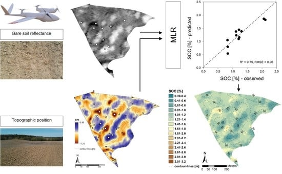
In this study we investigate the potential of UAS-based multispectral, high spatial resolution imagery in combination with a second-order terrain attribute for the prediction of SOC content at field scale. In terms of sampling strategy, we performed a parsimonious approach; i.e., we used a small dataset of ground-based measurements at two representative arable fields for model development. We compare local models with a model build from an enlarged dataset consisting of samples from both fields (pooled approach). In addition, by applying local models to the respective other field, the ability for cross-field prediction will be evaluated.

2. Materials and Methods

2.1. Study Area

This study was performed at the “AgroScapeLab Quillow” (ASLQ)—ZALF’s landscape laboratory covering 260 km² of the Uckermark region in NE Germany. The ASLQ is part of the Weichselian-age ground moraine landscape with a pronounced hummocky relief. This landscape type is quite important for global crop production as it covers ~10% of the arable land at the global temperate climatic zone [27,38].

Convex knolls and closed, concave depressions take turns over a short distance (50–100 m), which leads to strong local soil-moisture gradients (dry to wet in <100 m distance). The area is characterized by a subcontinental climate with a mean annual air temperature of 8.7 °C. Mean annual precipitation decreases from 550 mm in the western to 450 mm in the eastern part of the ASLQ (1990–2019, ZALF Research Station Dedelow; 53°21′55.46″ N/13°48′17.78″ E). Soils mainly developed from illitic-calcareous glacial till (sandy loam) and—to a minor portion—from carbonate-free, sandy sediments (glacial, glaciofluvial, periglacial). The actual soil pattern of the area is strongly affected by soil erosion over the past centuries [29,39,40,41]. Recent studies confirm the dominant role of tillage erosion compared to water erosion [40]. Only 20% of the arable land shows soils unaffected by soil erosion (Calcic Luvisols), mainly at lower midslopes. Extremely eroded soils (Calcaric Regosols) occur at convex landscape positions, especially hilltops (knolls), as well as on steep slopes. Strongly eroded soils (Nudiargic Luvisols) stretch from upslopes to upper midslopes. Footslopes and closed depressions comprise 20% of the landscape. Here, groundwater-influenced colluvial soils have developed (Gleyic-Colluvic Regosols, partly overlying peat). The study area is under intensive arable land use. Typical crops grown in the “ALSQ” are winter wheat (Triticum aestivum L.), winter canola (Brassica napus L.), maize (Zea mays L.), and winter barley (Hordeum vulgare L.). Soil erosion together with a strong wetness gradient leads to a very high spatial variability of growth conditions, hence crop biomasses [18].

The study was carried out at two contrasting arable fields of the ASLQ, designated as “hd02” (22 ha; central coordinate: 53°23′0.62″ N/13°46′53.68″ E) and “kr01” (16 ha; central coordinate 53°23′24.66″ N/13°39′16.95″ E) (Figure 1).

The two selected fields cover the full range in: (i) glacial till lithology (kr01 more clayey than hd02), (ii) intensity of soil erosion (kr01 < hd02) and (iii) soil wetness as derived from soil redoximorphism (kr01 > hd02) of the “ASLQ”. Elevation ranges between 48 m and 59 m above sea level (ASL) on field hd02 and between 81 m and 96 m ASL on field kr01. The topography of both fields is characterized by leveled to moderately sloping areas (hd02: 0°–14°; kr01: 0°–19°). All of these factors influence the SOC level.

2.2. Soil Sampling and Soil Analysis

Sampling locations at each field were selected according to pedological knowledge along an erosion-deposition gradient, which covers the full feature space in terms of soils’ SOC status. Topsoil samples (0–15 cm) in both fields (hd02: 11, kr01: 8) were taken at points for which auxiliary soil data were available from previous sampling campaigns. The points were formerly selected by a stratified-random-sampling scheme, which included the TPI, the Normalized Difference Vegetation Index (NDVI) from satellites (Quickbird, RapidEye) as well as the apparent electrical conductivity (ECa) from geophysical mappings (EMI 38) as strata. All strata are involved in landscape scale carbon cycling, hence influence SOC content in topsoils. Crop growth conditions, related C inputs and resulting SOC content and stocks are determined by erosion states of soils in hummocky ground moraine landscapes. Erosion state itself is reflected by terrain attributes, especially TPI in the case of tillage erosion, which is by far the most important mode of erosion in the study area. Spatial distribution of the ECa served as a proxy for the clay content as the most important subsoil property (water, nutrient supply). Finally, crop biomass derived from satellite imagery is directly related to C-inputs into soils and reflect local conditions in an integrated manner.

We carried out a composite sampling to capture the local, small-scale variability. Three topsoils in 1 m distance to the central coring point were sampled along a triangle and bulked into one sample (=physical averaging). The achieved average sampling density of one soil sample per two hectares depicts a low, but common sampling density of agricultural practice in NE Germany.

Bulk soil samples were air dried, gently crushed and sieved at 2 mm to separate the fine earth fraction (<2 mm) from the gravel (>2 mm). The particle size distribution of the fine earth was determined by a combined wet sieving (>63 μm) and pipette (<20 μm) method (DINISO 11277 1998). Pretreatment for particle size analysis was performed by wet oxidation of the soil organic matter using H₂O₂ (10 vol. %) at 80 °C and dispersion by shaking the sample end over end for 16 h with a 0.01 M Na₄P₂O₇ solution [33]. The total C content was determined by dry combustion at 1050 °C using an elemental analyzer (Vario EL, Elementar Analysensysteme). Soil inorganic carbon content (SIC, mainly CO₃–C) was determined conductometrically using a Scheibler apparatus [42]. The SOC content was calculated as the difference between total C and SIC. Pedogenic iron (Fe) oxides were characterized by dithionite (Fe_d) and acid-oxalate extraction (Fe_o) [42]. The Fe concentrations in the solutions were determined by ICP-OES. All basic soil analyses were performed in two laboratory replicates.

2.3. Topographic Position Index (TPI)

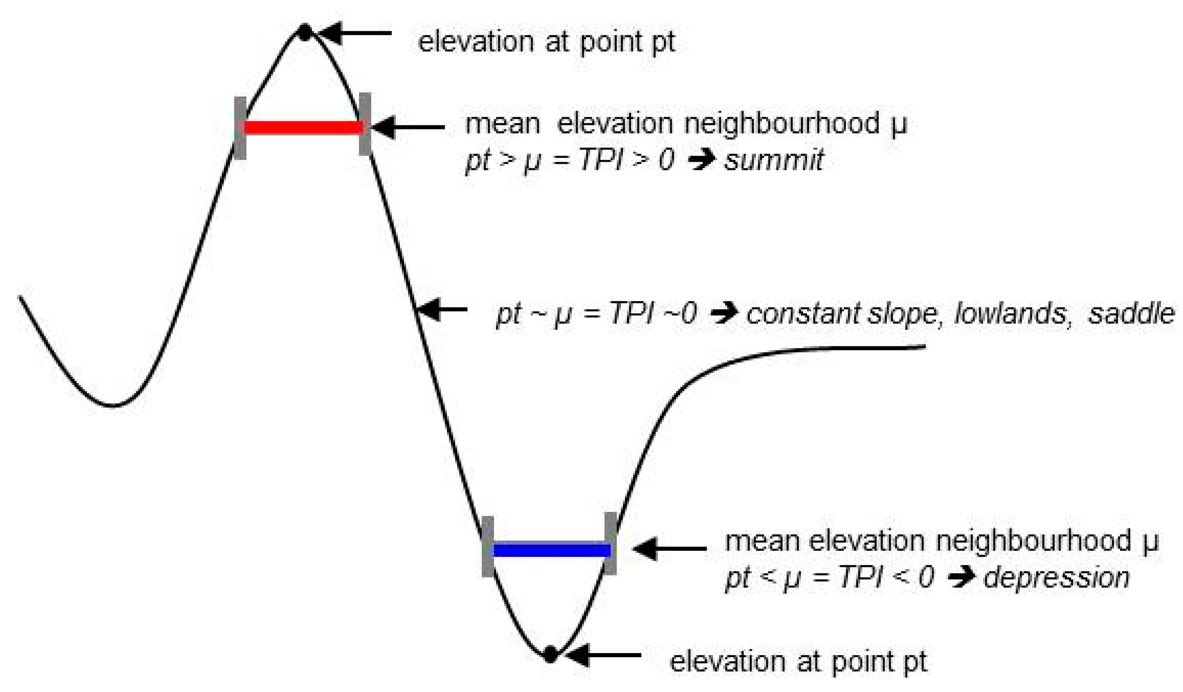
The TPI is the difference between the elevation of each grid cell in a DTM and the averaged elevation of a neighbourhood defined by circles of arbitrary radius. According to [43], the TPI for a single grid cell is calculated by:

$$\mathrm{TPI} = \left(h-\left(x_h\left(r\right)\right)\right)$$

(1)

where h is the elevation of a grid cell in meter above sea level, x_h is the mean elevation of grid cells in the neighbourhood with radius r. Values of the TPI range between −1 and +1 where negative values represent DTM grid cells lower than their surroundings and positive values higher ones, respectively (Figure 2).

At the time of UAS missions no GNSS (Global Navigation Satellite System) reference station was available that provides the required positioning correction data for the generation of a high precision DTM from simultaneously captured RGB images. The DTM used here was generated in accordance with the latest quality standards for the entire ASQL from a LiDAR (Light Detection and Ranging) airborne mission conducted in 2010 by order of the “Amt für Geoinformation, Vermessung- und Katasterwesen” (AfGVK, Federal state of Mecklenburg-Vorpommern). The original resolution of 1 m showed unwanted details and structures related to actual farming practices (e.g., tillage operations and tractor lanes). The DTM was resampled to a resolution of 5 m to smooth out these effects.

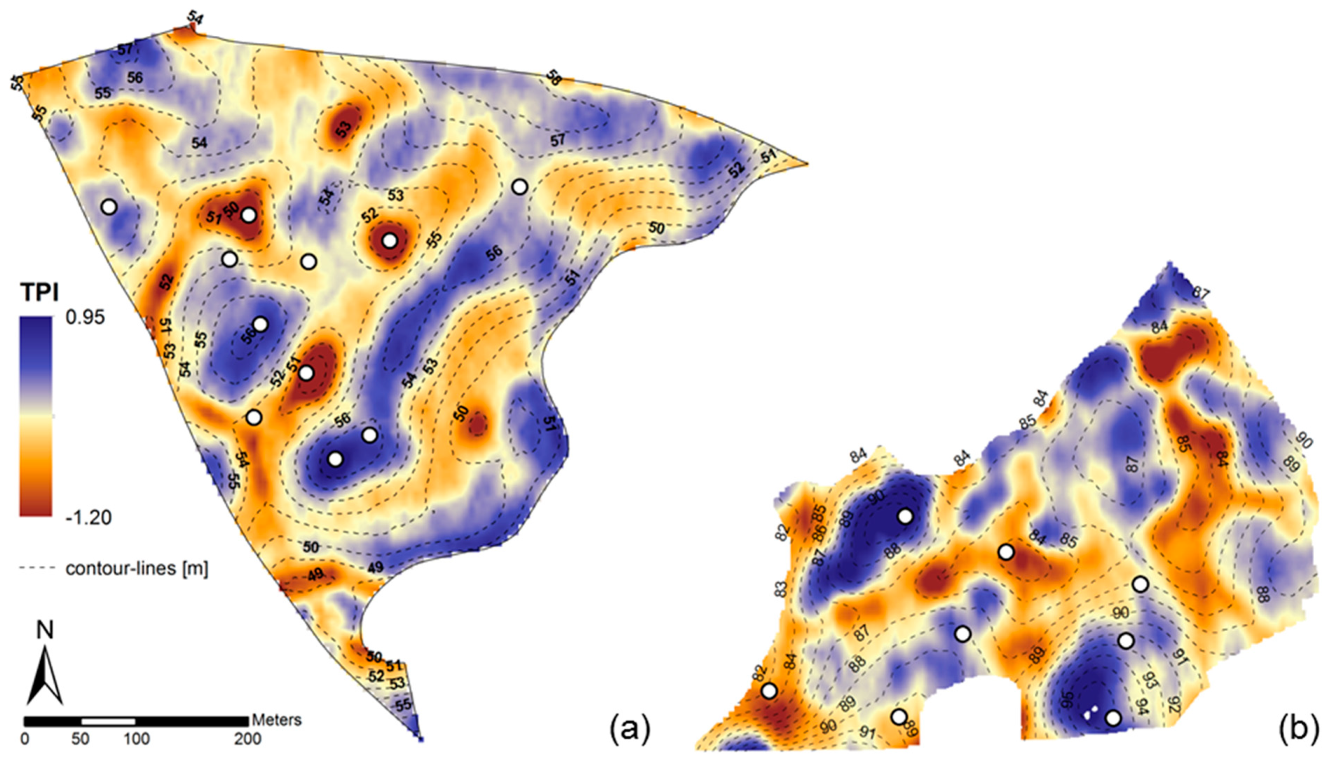
The ArcView extension “TPI” (Jenness Enterprises, Flagstaff, AZ, USA) was used to calculate the TPI for the entire ASLQ. A radius of 5 grid cells (25 m) was found to be appropriate for this landscape [44] to identify small relief elements (knolls, closed depressions) and related soil types within both fields (Figure 3).

2.4. UAS Remote Sensing

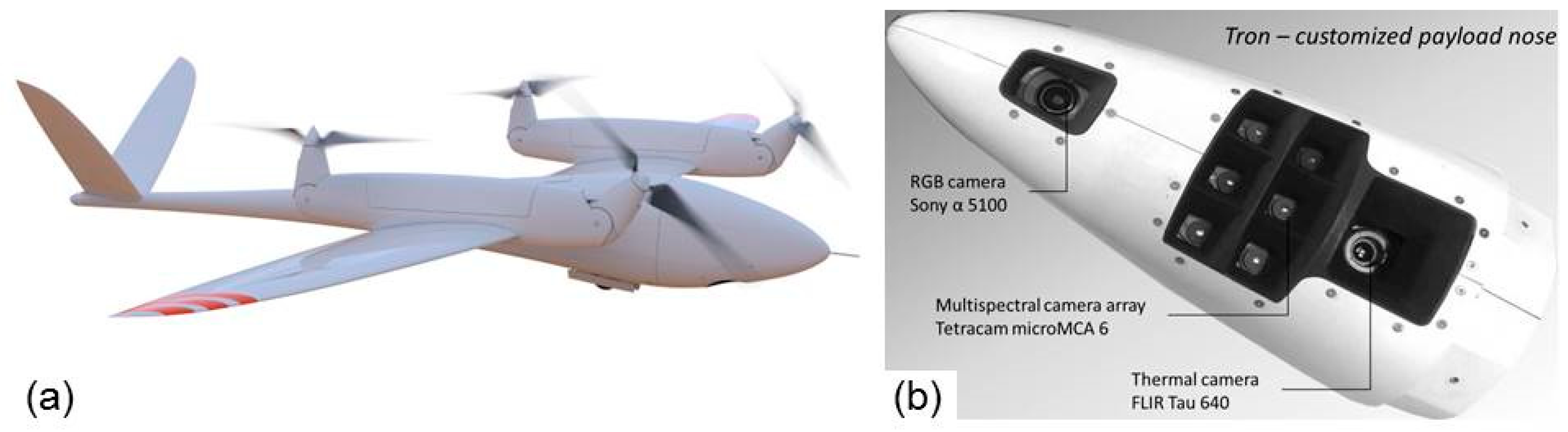
The fixed wing UAS Tron (Quantum Systems GmbH, Gilching, Germany) is a vertical take-off and landing (VTOL) system (Figure 4a). With a wingspan of 3.5 m and the four electric tiltrotors the Tron combines the benefits of both long-range aerodynamic flight capabilities up to 2 h and independency from airstrips in close distance to the flight area. The total take-off weight is about 14.5 kg including the camera payload of approximately 2 kg. The core of the sensor equipment is a miniature multi-camera array Mini-MCA 6 (MCA hereafter) (Tetracam Inc., Chatsworth, CA, USA) supplemented by a FLIR Tau 640 thermal camera incorporated in the same rugged chassis. The MCA consists of an array of six individual CMOS sensors (1280 × 1024 pixels; pixel size 5.2 µm), lenses (focal length 9.6 mm) and mountings for user defined, interchangeable band-pass filters. The six mounted narrow-band filters, manufactured by Andover (Andover Corp., Salem, MA, USA), cover the spectral range from visible to near infrared wavelengths (550 nm, 570 nm, 610 nm, 656 nm, 760 nm and 900 nm). The bandwidths range between 10 nm (the first five bands) to 40 nm (band 6). A skyward looking electronic incident light sensor (eILS) collects downwelling solar irradiation using an identical band filter set as mounted on the MCA. The eILS images are captured simultaneously to each MCA image and are used in the post-processing chain for radiometric calibration purposes. Camera lenses are partly covered by view caps, which narrow the field of view to minimize vignetting effects. An off-the-shelf 24 MP Sony alpha 5100 camera (Figure 4b) complements the sensor package. Both cameras are triggered by the Tron autopilot in a 2 s interval.

The missions were carried out at bare fields on 16 August 2018 (hd02) and 30 April 2019 (kr01) close to the respective maximum possible solar zenith angle. We chose a flight altitude of 200 m above ground to achieve a sufficient ground sampling distance of approximately 0.11 m. Sky conditions were cloud free and winds speeds were moderate during both missions. The images of field hd02 were partly affected by cloud shadows in the eastern part of the field and were excluded from further image processing. Both missions were carried out during a longer rain-free period a couple of days after the preparation of the sowing bed of subsequent crops.

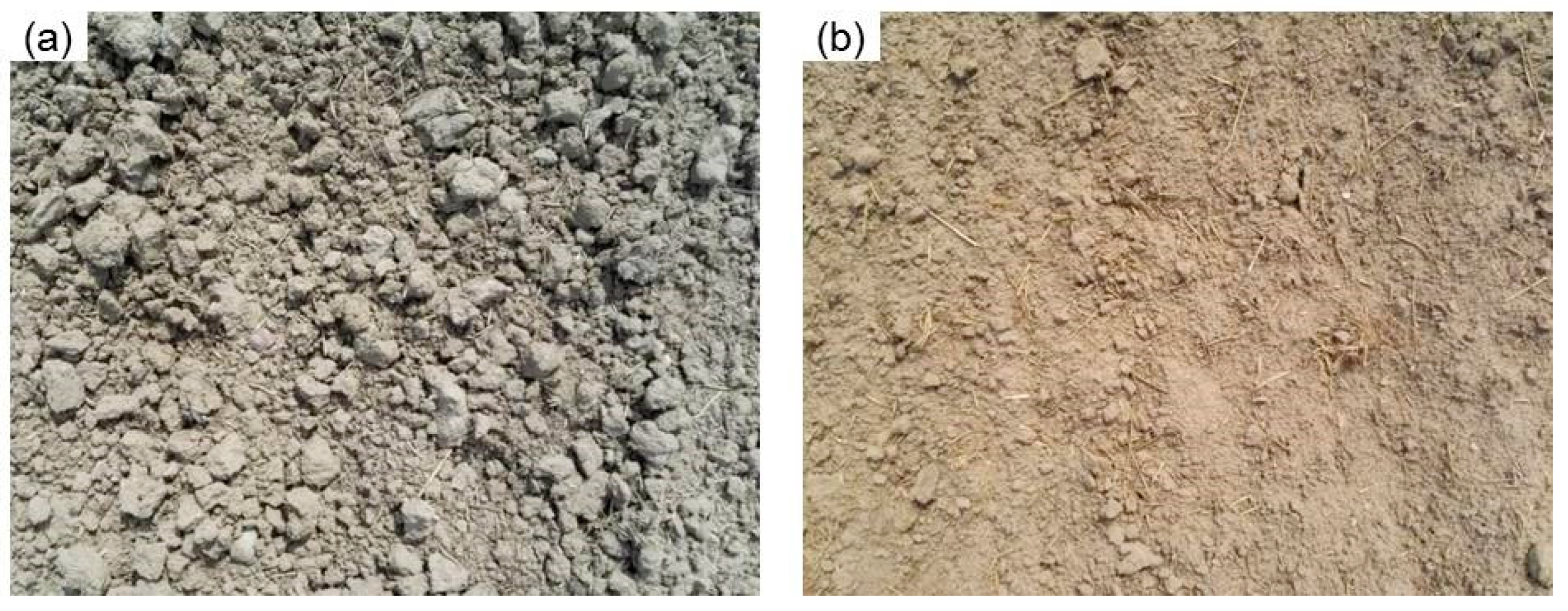
After milling and rolling, soil surfaces showed gentle roughness and little variation between the two fields but larger differences across different soil types. Soils with higher clay content formed larger soil aggregates (Figure 5a) than the sandier soils (Figure 5b) and showed respectively higher shading effects. Soil moisture in the upper 2 cm was low in almost all topographic positions with the exception of some small areas in the center of depressions.

Additionally, two of the depressions in field hd02 were rummaged by boars. The main difference concerning surface conditions on the two fields was caused by management effects. While field kr01 was almost free from crop residues, the surface of field hd02 was sparsely covered by straw residues of winter wheat. However, the coverage was higher in depressions, were proper seedbed preparation failed due to technical limitations of the cultivator or harrow.

2.5. Image Pre-Procesing

The retrieval of SOC from a bare soils surface requires an absolute calibration of the collected imagery because a recorded digital number (DN) is not only a function of the spectral characteristics of a bare soil surface but also of environmental conditions [45]. These include in particular the atmospheric conditions during the flight and the respective illumination geometry (solar zenith and sensor viewing angles). A straightforward way to convert DN to at-surface reflectance is the use of eILS measurements. An in-flight calibration of images using each corresponding eILS measurement showed unsatisfactory results clearly apparent by means of slight banding artefacts in the final mosaic of all calibrated images. Without having a reasonable explanation, the patterns disappeared with the use of a single eILS measurement selected by two criteria: (i) flight direction and (ii) flight attitude. We obtained best results by using an eILS measurement captured in flight direction towards the sun and almost no UAS movement along the pitch- and roll-axis (correspond to nadir-view conditions). We used the PhotoScan-Pro (V. 1.7.) software (Agisoft LLC, St. Petersburg, Russia) for image mosaicking. The workflow involves common photogrammetric procedures including the search for conjugate points by feature detection algorithms used in the bundle adjustment procedure, approximation of camera positions and orientation, geometric image correction, point cloud and mesh creation, automatic georeferencing and finally the creation of an orthorectified mosaic [46]. This workflow (lens distortion correction included) was applied to create an orthorectified mosaic from RGB images collected by the RGB camera (GSD ≈ 4.8 cm) and flight attitude data. The involvement of flight attitude data in the workflow produced discernable misalignments in the resulting multispectral MCA orthomosaic. Therefore, eILS-calibrated images captured by each MCA band were mosaicked individually. The GPS-measured positions of white markers (15 cm × 15 cm) were used to improve the spatial accuracy of the automatically generated RGB orthomosaic applying the ArcMap (V. 10.4.1) georeferencing tool. The orthomosaic was transformed to the local coordinate system ETRS 89 UTM 33, which finally served as a spatial reference for the co-registration of the six MCA orthomosaics. On average, 15 ground control points were sufficient to yield a co-registration accuracy between 1–2 pixels using a second order polynomial function. We used an ASD FieldSpec 4 Wide-Resolution spectrometer (ASD Inc., Boulder, CO, USA) to sample bare soil spectra directly after image acquisition. White reference spectra were collected before soil measurements using a Spectralon^® reference panel. Since the distance between fibre optics and soil was approximately 1 m, the collected spectra represented an average reflectance from a circle of 0.44 m in diameter. Measurements from all locations were acquired to check agreement with eILS calibrated MCA spectra. We then compared the averaged MCA reflectance at ASD sample locations (5 × 5 pixels) with mean ASD reflectance sampled in respective MCA bands according to bandwidth.

2.6. Spectral Band Selection

Due to the limited numbers of samples, a simple Multiple Linear Regression (MLR) model was used to predict SOC content. The TPI as a stand-alone predictor was not considered to be an appropriate explanatory variable for SOC content, nor for the pooled approach or the cross-field predictions since the same TPI values may correspond with different SOC content in other fields caused by slightly different soil properties (e.g., clay content) or management (e.g., fertilization). To avoid overfitting, only one spectral band, together with the TPI, was selected by a leave-one-out-cross-validation (LOOCV) using the hydroGOF package in R software (R development Core Team, Vienna, Austria). To assess accuracies and predictive power of the models built from the respective covariates, the coefficient of determination (R²), the Root Mean Square Error (RMSE; Equation (2)) and the Ratio of Performance to Interquartile Range (RPIQ; Equation (3)) were computed for both the pooled approach and the two individual fields. We evaluated the contribution of the TPI to the model performance by repeating the LOOCV for the three single bands without the TPI as a covariate. Analysis of variance (ANOVA) was applied to assess the significance of model improvement by the TPI.

$$\mathrm{RMSE} = \sqrt{\frac{{\sum }_{i=1}^n\left(y_o-y_p\right)²}{n}}$$

(2)

$$\mathrm{RPIQ} = \frac{\mathrm{IQ}}{\mathrm{RMSE}}$$

(3)

where y_o and y_p are observed and predicted values and n is the number of data pairs. IQ is the difference between Q3 (values below 75%) and Q1 (values below 25%) of the sample distribution. Due to the small dataset, no upper and lower limits for IQ were set, which usually detects outliers. Finally, the variance inflation factor (VIF; Equation (4)) was calculated to examine multicollinearity among predictor variables for the best performing variable combination.

$${\mathrm{VIF}}_j = \frac{1}{1-R_j{}^2}$$

(4)

where R_j² is the R² value obtained by regressing the j^th predictor on the remaining predictor. A VIF value of 1 indicates no correlation among predictor variables whereas values larger than 5 are suggested for detecting multicollinearity. However, there is no general agreement regarding a threshold value clearly indicating serious multicollinearity [47].

3. Results

3.1. Site Properties

Descriptive statistics of relevant site properties are summarized in

Table 1. Descriptive statistics of topsoil properties and the Topographic Position Index (TPI) of the pooled and field-specific datasets. Note: SOC and SIC data were sampled in the year of image acquisition, Clay content and, pedogenic iron oxides (Fe_d and Fe_o) were determined using soil samples collected in a previous sampling campaign.

Site Properties	Dataset	n	Mean	SD	Min	Max	Range	CV [%]	IQ
SOC [%]	pooled	19	1.5	0.6	0.8	3.0	2.2	37.7	0.5
	kr01	8	1.7	0.6	1.0	3.0	2.0	33.8	0.2
	hd02	11	1.3	0.4	0.8	2.1	1.3	35.4	0.3
SIC [%]	kr01	8	1.5	3.4	0.1	9.9	9.8	221.4	0.5
	hd02	10	2.7	3.6	0.3	12.2	11.9	133.1	3.4
Clay [%]	kr01	7	15.6	6.1	8.4	26.5	18.1	39.2	11.1
	hd02	10	13.9	4.5	6.2	20.8	14.7	32.4	4.7
Fed [mg kg−1]	kr01	7	4566	2288	1617	8148	6531	50.1	2936
	hd02	10	3853	1075	2212	6120	3908	27.9	928
Feo [mg kg−1]	kr01	7	1723	600	721	2438	1717	34.8	766
	hd02	10	1240	634	715	2403	1688	51.1	508
TPI	pooled	19	0.00	0.45	−1.00	0.80	1.80	13190.9	0.49
	kr01	8	0.10	0.38	−0.40	0.80	1.20	396.8	0.43
	hd02	11	−0.06	0.50	−1.00	0.69	1.69	796.7	0.55

. The SOC content in the upper 15 cm ranged from 0.8% at strongly eroded hilltops (field hd02) to 3.0% at the center of a depression (field kr01). Within field variation was higher at field kr01 due to the high SOC content in the central depression, which is a periodically flooded (former) kettle hole.

3.2. Image Processing

The mosaicking procedure failed for the eILS-calibrated images captured in bands b610 and b656 of the hd02 mission exactly for the relevant part of the field containing most of the sampling points. Although MCA reflectance values agreed well with ASD values in the single images (data not shown), we excluded both bands from further evaluation. ASD spectra of the remaining bands (b₅₅₀, b₅₇₀, b₇₆₀ and b₉₀₀) revealed inconclusive results. Bands b₅₅₀ and b₅₇₀ were in good accordance with ASD values for both fields. Mean differences ranged between −0.007 and 0.008 (field kr01) and 0.027 and 0.014 (field hd02) for b₅₅₀ and b₅₇₀, respectively. On average, band b₇₆₀ matched perfectly for field kr01 but showed a considerable difference (0.055) at field hd02 (Figure 6). The worst agreement existed for the NIR band b₉₀₀. MCA values exceeded ASD values to more than 100% suggesting a systematic error in the calibration file shipped with the camera and was therefore rejected. The scatterplot of the remaining three bands indicated slightly higher MCA reflectance for the hd02 mission in the VIS bands and a generally lower dynamic range in all MCA bands compared to ground measured ASD values.

3.3. Predictor Selection and Statistical Analysis

Regarding the statistical measures produced by the LOOCV, b₅₇₀ was found the best predictor for SOC in all evaluated approaches regardless of using a single band or in conjunction with the TPI (

Table 2. Results of the leave-one-out-cross-validation (LOOCV) of evaluated SOC prediction models expressed by the coefficient of determination (R²), the Root Mean Square Error (RMSE) and the Ratio of Performance to Interquartile Range (RPIQ). Values showing the highest prediction performance regarding the RPIQ are highlighted.

	Local kr01			Local hd02			Pooled
Predictors	R²	RMSE [%]	RPIQ	R²	RMSE [%]	RPIQ	R²	RMSE [%]	RPIQ
b550	0.81	0.26	2.47	0.37	0.37	0.82	0.55	0.36	1.34
b570	0.84	0.24	2.72	0.52	0.30	0.82	0.60	0.34	1.42
b760	0.10	0.55	0.29	0.33	0.35	0.82	0.27	0.46	1.05
b550, TPI	0.86	0.12	3.89	0.39	0.37	0.84	0.65	0.33	1.47
b570, TPI	0.91	0.11	4.27	0.48	0.33	0.84	0.73	0.28	1.73
b760, TPI	0.62	0.36	0.44	0.41	0.35	0.84	0.63	0.32	1.51

). Among the control variants without the TPI, the local model for field kr01 produced the lowest prediction error and showed the highest prediction ability (RMSE = 0.24%; R² = 0.84; RPIQ = 2.72). Despite the use of all 19 samples (pooled approach), the prediction performance decreased significantly (RMSE = 0.34%; R² = 0.60; RPIQ = 1.42), but outperformed the local hd02 model (RMSE = 0.30%; R² = 0.52; RPIQ = 0.82). By adding the TPI as a second explanatory variable, all measures computed for the local model kr01 indicated an increased prediction accuracy (RMSE = 0.11%; R² = 0.91 and RPIQ = 4.27). Regarding the prediction performance, the effect was less pronounced for the field hd02 model, where the RPIQ was slightly higher (RPIQ = 0.84 vs. 0.82), but the RMSE increased from 0.30% to 0.33%. In contrast, the TPI improved the prediction performance and accuracy for the pooled data (RMSE = 0.28%; R² = 0.73; RPIQ = 1.73).

Correlations among the most successful predictor variables b₅₇₀ and TPI were moderate for the local models (field kr01: R² = 0.61, field hd02: R² = 0.61) and low for the pooled dataset (R² = 0.14). Calculated VIF values of 2.54 (field kr01), 2.56 (field hd02) and 1.16 (pooled dataset) indicated no serious multicollinearity.

The ANOVA showed a minor but significant (p < 0.01) deterioration of the model performance when the TPI was included. Nonetheless, regarding the small number of samples and the respective distribution especially on field kr01, the results of the LOOCV were highly sensitive to the prediction of samples marking the upper and lower tail of the SOC range.

3.4. Spatial Distribution of SOC

According to the better prediction performance using the TPI, the spatial distribution of SOC content was computed using the MLR with the two predictor variables b₅₇₀ and TPI. We compared the mapped SOC content (local versus pooled) to assess quantitative differences and the impact on the spatial distribution apart from performance metrics when using a small rather than a large number of samples. Furthermore, we evaluated the ability of the local models for cross-field predictions.

3.4.1. Comparison of Local Models with the Pooled Approach

R²s and RMSE for each approach are given in

Table 3. Coefficients of determination (R²) and Root Mean Square Errors (RMSE) of the local (fields kr01, hd02) and the pooled approach build from reflectance at 570 nm and the Topographic Position Index (TPI).

Dataset	n	R²	RMSE [%]
kr01	8	0.88	0.07
hd02	11	0.79	0.06
Pooled	19	0.86	0.05

and corresponding model equations are given in

Table 4. Multiple Linear Regression (MLR) models for the local approach (fields kr01, hd02) and the pooled approach build from reflectance at 570 nm and the Topographic Position Index (TPI).

Dataset	Model Equations
kr01	$\mathrm{SOC} [\%] = \left(-22.32\times b_{570}\right)+\left(-0.51\times TPI\right)+4.66$
hd02	$\mathrm{SOC} [\%] = \left(-19.01\times b_{570}\right)+\left(-0.37\times TPI\right)+4.24$
Pooled	$\mathrm{SOC} [\%] = \left(-19.78\times b_{570}\right)+\left(-0.43\times TPI\right)+4.43$

. The respective relationships between predicted and observed SOC are shown in Figure 7a,b. The R²s ranged between 0.79 (field hd02) and 0.88 (field kr01). The low RMSE values between 0.05 and 0.07 indicated high prediction accuracy.

Figure 8a,b depicts the spatial distribution of SOC computed from the local models for field hd02 and kr01, respectively. Regardless of the higher level of SOC content on field kr01, the spatial distribution clearly showed a general accordance with terrain. However, in contrast to field hd02, higher SOC content occurred in up- and midslope positions on field kr01 (e.g., points 11 and 13), which hardly fell below the content in the central depressions. This might be related to the dominance of stagnant water soils, which are known to reveal higher SOC in topsoils due to: (i) O₂ deficiency during wetter periods (inter-/intraannual) and (ii) higher C sorption capacity of newly formed, amorphous Fe oxides (redox processes).

Compared with observed values, highest prediction errors occurred at the lower and upper tail of the SOC range. At both tails, SOC was underestimated by the local models in extreme terrain positions (e.g., point 25 on field hd02; hilltop, point 5 on field kr01; hilltop, point 0 on field kr01; depression). Overestimations occurred at points in transitional terrain positions with medium SOC content (e.g., point 33 on field hd02; footslope, point 14 on field kr01; midslope). The MLR developed from all 19 points from both fields (R² = 0.86; RMSE = 0.05%) revealed no improvement of the prediction accuracy compared to the local models regarding SOC levels and the spatial patterns. The relative accuracy, calculated as the difference between the models, was negligible for field hd02 and showed deviations lower than ±0.1% SOC (Figure 9a). Less than 2% of the area showed larger deviations again occurring in extreme terrain positions (central depression and one of the hilltops) of field kr01 (Figure 9b). However, the comparison with observed SOC values at point level indicated an outperformance of the local models at the upper and lower tail of the SOC range. With the exception of point 5 on field kr01, predicted content clearly exceeded the errors produced by the local models unless a larger dataset was used.

3.4.2. Cross-Field Prediction Ability

The local model developed for each field was used to predict SOC content in the topsoil of the respective other field. Despite the smaller influence of the TPI on field hd02, the application of Equation (4) (field kr01) to field hd02 data showed a high correlation between cross-field predicted and observed SOC content (Figure 10) but tended to underestimate lower values.

Regarding the difference between the local model and the cross-field prediction, the underestimation is larger than 0.1% for 60% of the total field area (Figure 11a). Nevertheless, SOC content was underestimated by only 9.6% (absolute 0.11%) on average. As observed for the local model, the largest difference between predicted and observed values occurred at point 25 (0.27% and 0.83%, respectively), compared to the local model the prediction error which increased significantly from −0.29% to −0.56% SOC. In contrast, the differences for higher SOC content were negligible (e.g., point 33; local 0.24%, across-field 0.22%). The cross-field prediction of SOC content on field kr01 using Equation (5) showed minor differences regarding the spatial distribution and the SOC level. The deviation, depicted in Figure 11b, ranged between −0.1% and 0.1% SOC for 96% of the field area compared to the local model.

SOC content was underestimated in the central depression, where the prediction error, represented by point 0, increased from −0.29% to −0.45%. The larger dark colored area in the surrounding of point 5 indicated an overestimation towards the local model. As already observed for the pooled approach, the prediction error produced by the local model was larger than the error produced by the across-field prediction. The difference between predicted and observed SOC content at point 5 decreased from −0.28% to −0.07%. Since the error for transitional terrain positions (e.g., point 14) equaled more or less the error produced by the local and the pooled approach, the cross-field prediction performed equally well for the major part of the field area and even outperformed the local model on eroded hilltops with low SOC content (point 7).

4. Discussion

We presented a simple multivariate approach for the prediction of spatially distributed SOC content in topsoils at the agricultural field scale incorporating soil reflectance data by UAS remote sensing and topography, based on a small dataset of ground-based measurements. Unfortunately, among the six MCA bands, only three bands were available for SOC prediction in topsoils of both fields showing sufficient calibration quality and full spatial coverage. However, we found the highest prediction ability according to the LOOCV statistics for the two local models and the pooled approach for the reflectance at 570 nm, irrespective of using the reflectance as a single predictor variable or together with the TPI as an independent covariate. Regardless of remote sensing platforms, sensors, scales and data evaluation techniques used in previous studies, our results generally confirmed the suitability of spectral bands located in the VIS-NIR wavelength domain, provided that sensors are not equipped with spectral bands in the SWIR region. Since SOC exhibits no specific absorption features in this spectral region the reported results reflected the simple relationship between soil colour and reflectance—the higher the SOC content, the lower the reflectance.

However, a bundle of factor combinations is known to modify surface reflectance (e. g., soil type, surface and atmospheric conditions) and the variety of available sensors (including non-imaging spectroradiometers) provides reflectance data with different spectral and spatial resolutions. Consequently, a range of spectral bands between 400 and 700 nm were used successfully for SOC prediction. A significant influence of SOC content on reflectance of different soils using spectroradiometers was reported for the VIS wavelength domain (550 to 700 nm, SOC range 0.8% to 9.0%) [10]; 500 to 700 nm, SOC range 0.1% to 4.0% [48]; around 600 nm, SOC range 0.2% to 40.2% [3]). Several statistical measures (Variance Importance in Projection (VIP) and factor loadings from Partial Least Square Regression (PLSR) technique or Relative Importance (RI)) were calculated to identify the most important spectral regions in multi- and hyperspectral data. Similar results were found for different spaceborne sensors [49], (SOC range 0.1% to 16%) and airborne HyMap spectra [50]; (SOC range 1.1% to 3.9%), [51] (SOC range 1.1% to 3.0%). Recently, a comprehensive study was conducted to compare current multi- and hyperspectral sensors (including a UAS-mounted multispectral camera) with respect to their SOC prediction ability for soil samples of the same field (SOC range 0.8% to 2.6%) and found the most important spectral bands, less precise, in the VIS-NIR region [20].

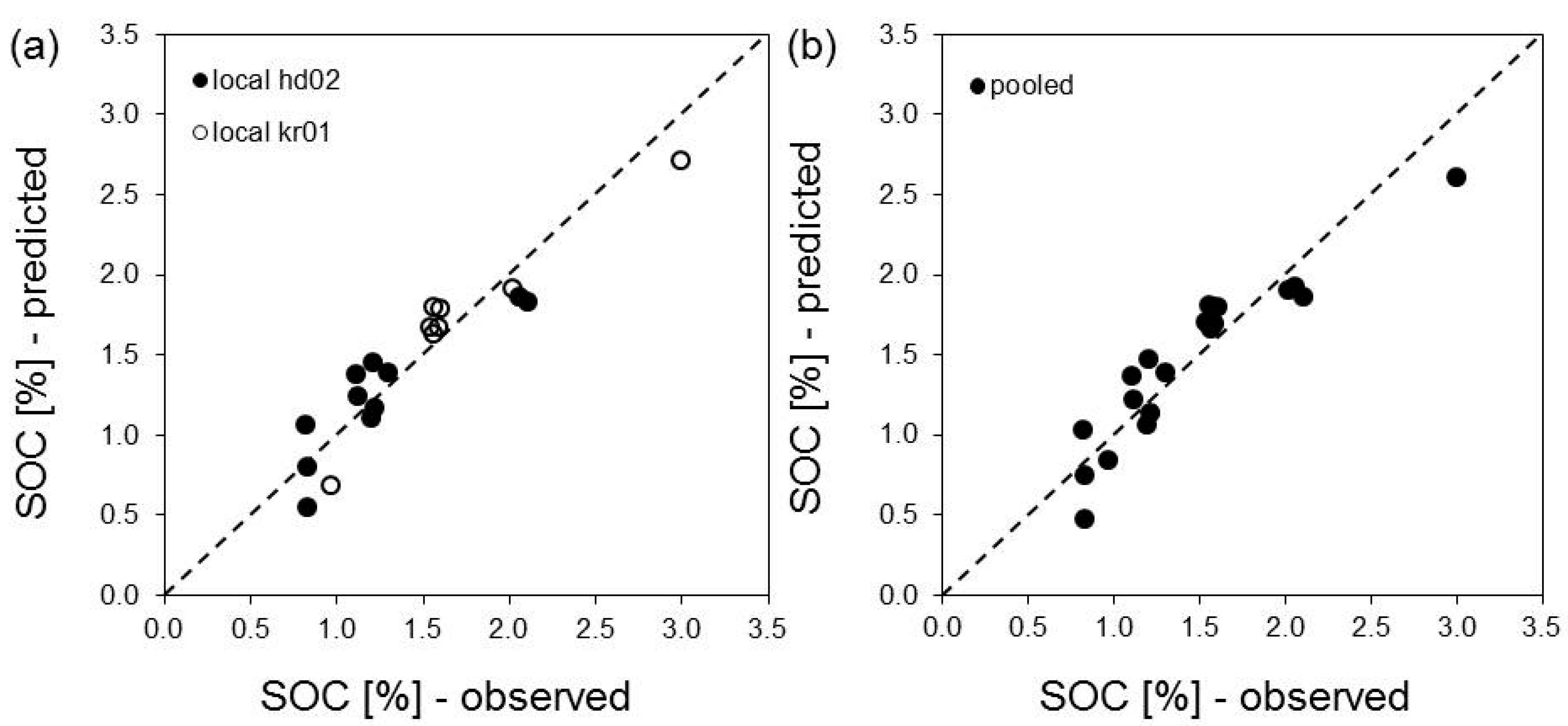
Using only the reflectance at 570 nm, our prediction performance showed satisfying results in terms of statistical metrics of the LOOCV especially for field kr01 (RMSE = 0.24%, RPIQ = 2.72). Remarkably worse values were found for field hd02 (RMSE = 0.30%, RPIQ = 0.82). If reported, aforementioned authors found similar prediction accuracies in terms of RMSE between 0.16 and 0.50 but RPIQs ranged between 1.53 and 3.34 (only reported by [20,48]. The performance of the UAS-mounted multispectral camera (Parrot Sequoia, 4 spectral bands) was slightly lower (RMSE = 0.31%, RPIQ = 1.77) compared to all other sensors. Better results were achieved by an earlier UAS mission conducted over bare soils of a field trail (SOC range 0.5% to 4.7%) at Rothamsted Research (Harpenden, UK) using a Tetracam Mini-MCA6 (RMSE = 0.21%, RPIQ = 2.3) [21]. However, results of most studies based on a larger number of observations compared to our approach, which in turn increased the model performance. This was partly confirmed by our pooled approach. Here, the RPIQ increased to 1.42, which is higher than the RPIQ obtained for field hd02, but lower than the value for field kr01. Nonetheless, the prediction accuracy decreased (RMSE = 0.34%) compared to the local approach. As proposed by different authors [17,20], the prediction accuracy might be improved by incorporating other environmental covariates into prediction models. By using the TPI in our study, the prediction error clearly decreased, and the model performance clearly increased in case of field kr01 (RMSE = 0.11%; RPIQ = 4.27). The RPIQ increased only slightly for field hd02 (RPIQ = 0.84 vs. 0.82 without TPI). For the pooled approach, the prediction error decreased (RMSE = 0.28% vs. 0.34% without TPI) and the RPIQ indicated a clearly better performance when using the TPI as an explanatory covariate (RPIQ = 1.73 vs. 1.42 without TPI). In conclusion, our results are in the range of worst and best model performances achieved by aforementioned studies.

The generally positive impact of the TPI was clearly related to the pronounced hummocky terrain of our study area. Convex and concave terrain features take turns over short distances and selected sample locations almost covered the full range of possible TPIs (−1 to +0.8). The close relationship between terrain position and SOC was founded in soil redistributions by tillage erosion [24,52,53]. Nevertheless, the TPI should be used carefully because values represent a spatially demarcated terrain attribute calculated from the immediate vicinity of a single grid cell. Therefore, limited conclusions can be drawn on the spatial dimension of, for example, a depression, which in turn determines the amount of locally sequestrated or relocated (by erosion) SOC. Hence, higher SOC content may occur in the center of wide, flat depressions as observed for point 0 on field kr01 (TPI = −0.4; SOC = 3%) than in small ones as observed for point 29 on field hd02 (TPI = −1.0; SOC = 2%). Therefore, the TPI is not suited for SOC prediction purposes without spectral covariates. Our MLR for spatial prediction of SOC content achieved high correlations and low prediction errors (field kr01: R² = 0.88, RMSE = 0.07%; field hd02: R² = 0.79, RMSE = 0.06%) showing similar intercepts and coefficients for the 570 nm band and the TPI.

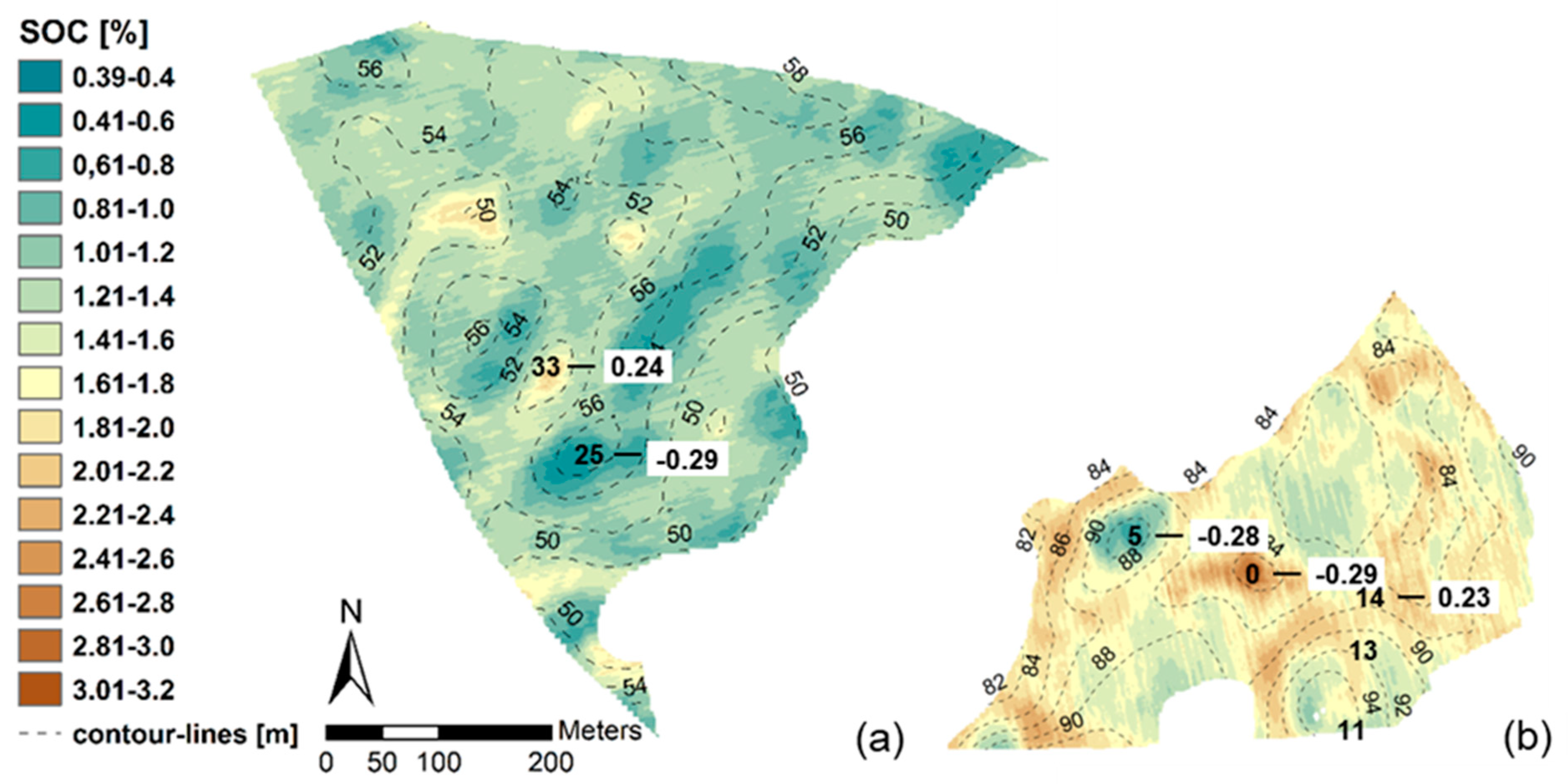
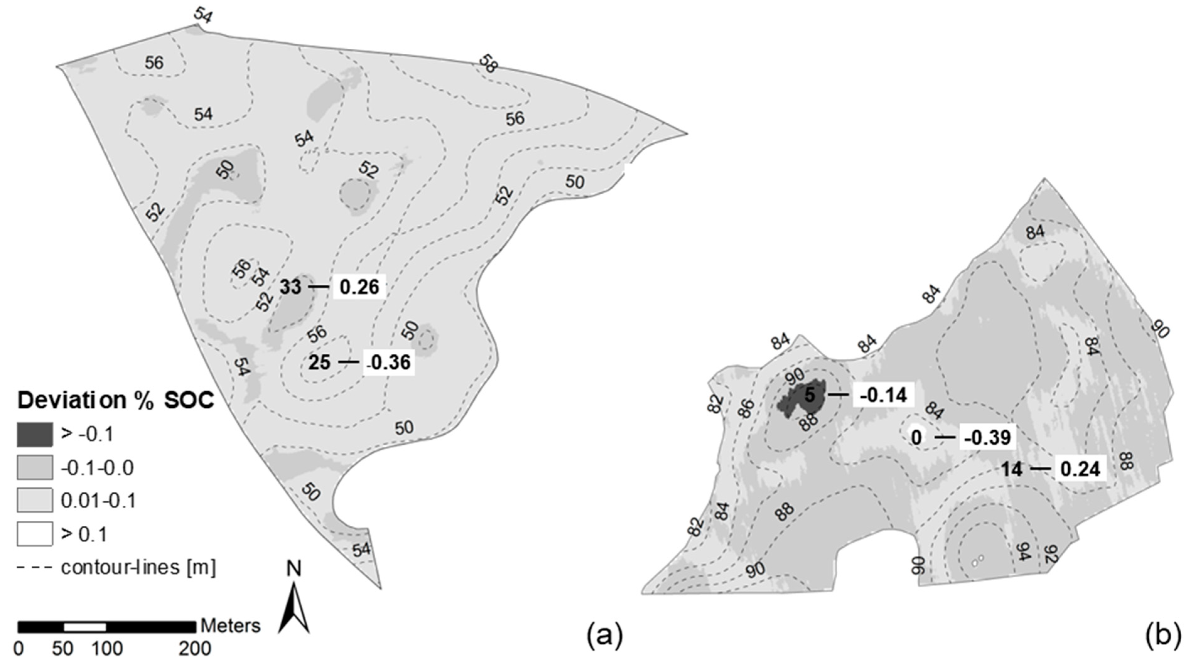
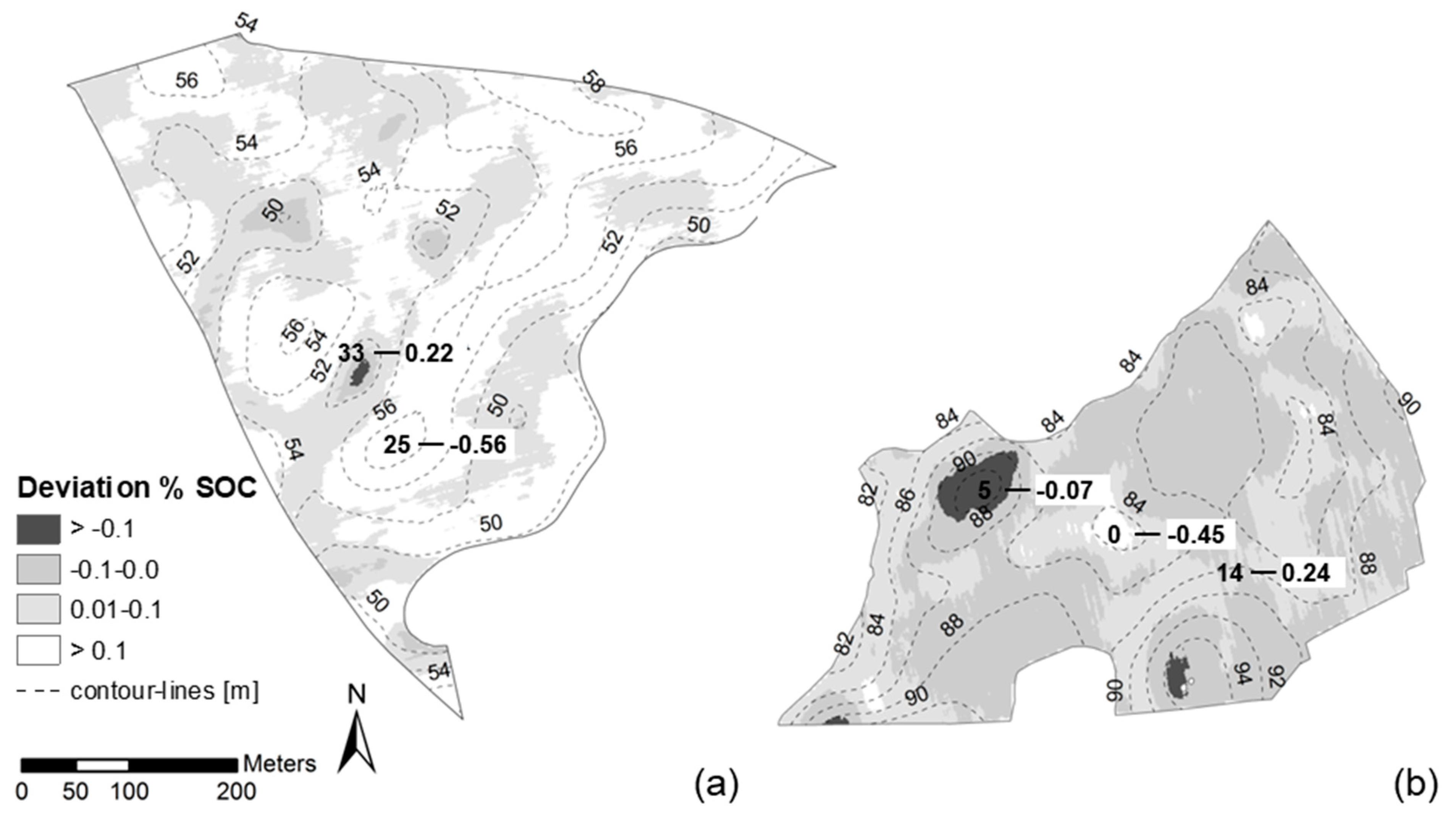
As expected, the resulting maps preferentially showed a pattern of SOC content, which was consistent to topography. The highest errors regarding individual sample locations occurred in depressions (high SOC content) and hilltop positions (low SOC content), where observed SOC content was underestimated in both fields. The first case was also observed in two studies using high spatial resolution UAS imagery: for Colluvic Regosols in depressions and weakly eroded Chernozems [20] and for field trials with long-term applications of organic manure [21].

For hummocky soil landscapes, we assume decreasing SOC content with depth in topsoil. While observed SOC represent the average content in the sample depth (topsoil), the spectral reflectance complies with the SOC content at the surface (~2 cm). Assuming a homogeneous uniform SOC distribution in topsoil of Colluvic Regosols and a continuous decrease in other soils, the surface reflectance will yield SOC values closer to the average for Colluvic Regosols. Consequently, the surface reflectance tends to overestimate average SOC content of other soil profiles rather than underestimate those of Colluvic Regosols. So far, the assumption of [21] was likely, since most SOC values in this study were low or medium. The underestimation of SOC content in strongly eroded hilltop positions at points 25 (field hd02) and 5 (field kr01) appeared to be related to soil mineralogy. The soil analysis showed that both points had remarkable high SIC content (12.2% and 9.9% respectively) compared to the average for all other points (1.8% on field hd02 and 0.4% on field kr01), which in turn increased reflectance in the VIS region [9,10]. Compared with soils having low SIC but similar SOC content, a disproportionate high reflectance probably decreased the predicted SOC content at these points. In our study there was no evidence for a significant effect of other surface properties such as roughness and straw residues. We consider these effects to be negligible compared with uncertainties related to spectral data, the TPI and the laboratory SOC determination. Finally, our sample design was not dedicated to the evaluation of these effects and thus most of them remained unaffected.

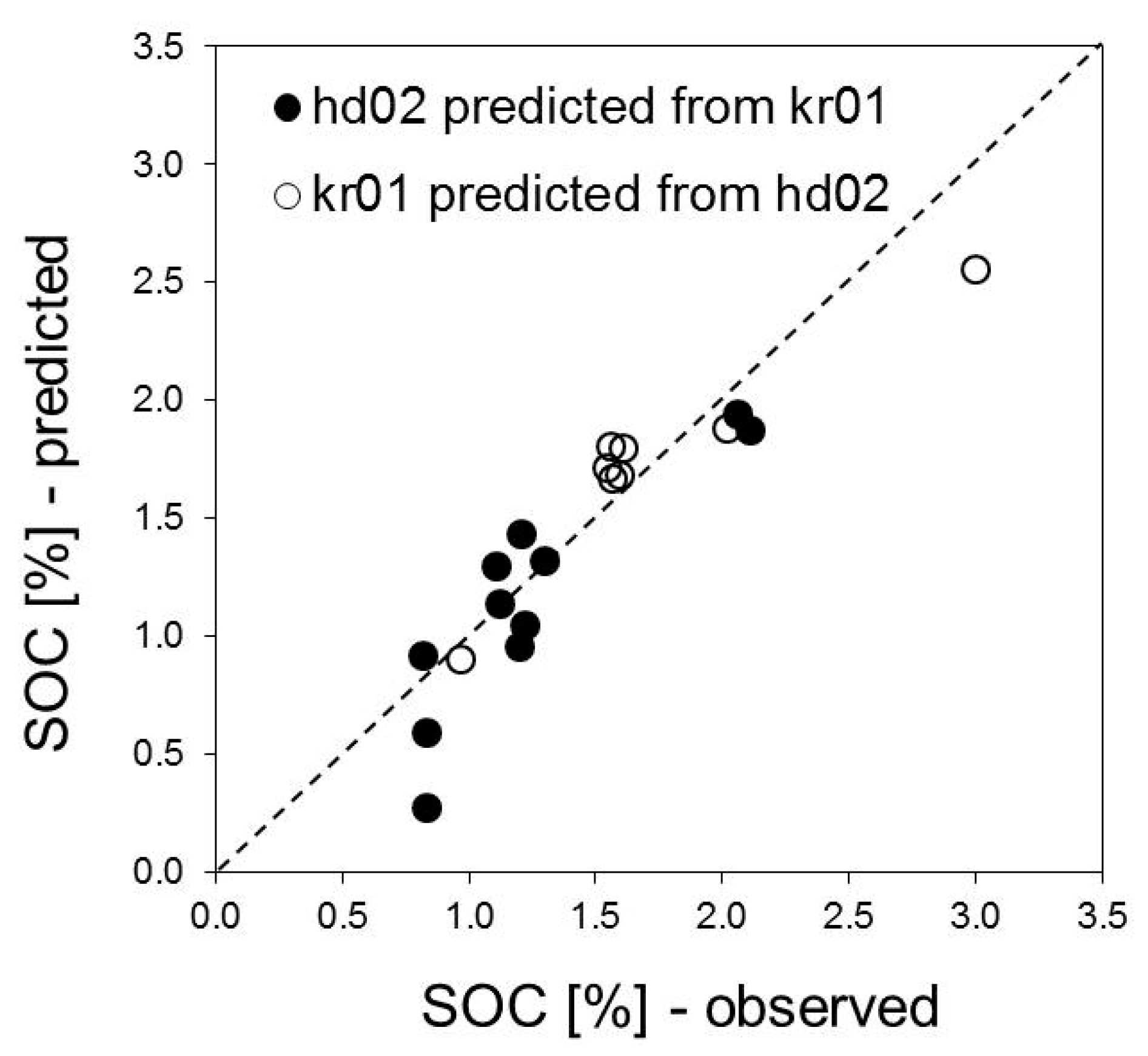
One of the most interesting issues is the ability of local models for reliable cross-field predictions of SOC content without having any information than spectral data and, if available, environmental covariates of explanatory value. Our results are promising, since deviations between local models and the respective cross-field prediction were negligible concerning the spatial distribution, the overall level and finally the SOC prediction of individual samples. From this, we conclude that the selected samples represent well the overall SOC range of both fields. Although a larger number of samples would probably increase the prediction accuracy, there was no evidence for a lack of samples representing other constellations of soil and topography than the selected.

Although soils showed a wide range of properties in terms of texture and mineralogy on both fields, the spectral response to SOC content was similar. Despite of higher calcium carbonate and lower iron oxide content on field hd02, soils developed under the same climatic conditions from the same parent material and were managed over a comparable time period. Insofar, our results are not surprising and support the findings and subsequently recommendations of other authors to stratify soils, sampled at regional or larger scales, according to their soil forming factors and management regimes yielding higher prediction accuracies compared to global calibration approaches [16,17,54].

Our approach is easily transferable and applicable in soil landscapes showing a similar geomorphological setting and tillage erosion as a major driver of soil distribution. As already stated in the introduction, this includes all landscapes of hummocky ground moraines, which cover approximately 1 Mio. km² arable land world-wide (Sommer et al., 2004). It will also work out in landscapes, where a strong contrast in SOC is explainable by a terrain-related interaction of geomorphic and pedogenic processes influencing carbon dynamics. The inclusion of the TPI as explanatory variable should be tested in further areas dominated by tillage erosion. However, the TPI will not improve the prediction of SOC content by remote sensing techniques on flat terrain, where other environmental conditions are considered as driving factors for spatial differences (e.g., parent material, hydrological conditions). For soil erosion by water, the Topographic Wetness Index (TWI) might outperform the TPI as the TWI will reproduce spatial domains of overland flow more robust. For wind erosion, a 3D DEM was used to capture luv-lee effects on wind speed and related sink-source domains of dust [55,56].

5. Conclusions

Our approach offers a high potential for spatially distributed SOC predictions from UAS remote sensing and generally available environmental covariates. This especially holds true for areas of limited soil data. A successful application of our approach requires a targeted selection of sampling locations. Coring points need to represent the full range of soils and related drivers (soil forming factors and processes), i.e., they need to cover the full feature space. Furthermore, we emphasize the great importance of optimized conditions during image acquisition, mainly soil surface characteristics. We strongly recommend the avoidance of high roughness (e.g., after ploughing) causing strong contrasts between illuminated and shaded areas. Reflectance of dead plant material such as straw and stubbles can hardly be distinguished from soil reflectance and thus increases uncertainties in SOC predictions. This is more important than a huge number of soil samples, predictor variables or sensor specifications. In this landscape type, which is characterized by predominately conventional agriculture, the chance for optimal conditions is best fulfilled during a time period (approximately 10 days) after seed bed preparation. Conducting flight and field campaigns by minimizing effects obscuring the relationship between spectral data and SOC content even enable reliable cross-field prediction accuracy.

Beside the basic issues concerning the natural (physical and biological) processes controlling SOC content, this demand is directly linked to the question of how farmers can react in a site-specific manner on small-scale varying and increasing SOC losses. Regardless the high spatial resolution, the spatial coverage is a general limitation even for fixed-wing UASs due to actual legal and technical restrictions, but sufficient for addressing an agricultural monitoring for at least two reasons.

First, considering the importance of framework conditions, agricultural landscapes consist of many fields but only few of them offer ideal conditions at the same time due to management practice (e.g., crop rotation, seedbed preparation, crop residues), soil moisture and surface roughness. Hence, simultaneous SOC predictions for numerous agricultural fields (e.g., from satellite imagery) require detailed information of surface conditions and local corrections. This, in turn, relativizes the advantage of the large spatial coverage provided by space-borne sensors.

Secondly, the application of UAS remote sensing is feasible even for the monitoring of changes in SOC content since loss and accumulation are long-term processes showing minor changes from year to year even on intensively managed agricultural fields. The detection of significant changes beyond the level of laboratory accuracy requires low repetition rates in the order of magnitude of years. Most disadvantages associated with the use of UASs, and mounted sensors are of technical nature. However, rapid technical progress provides more and more enhanced: (i) UASs with extended flight endurance and high accurate positioning capabilities by using real-time or post-processed kinematic and (ii) sensors equipped with in-flight calibration techniques and lower signal-to-noise ratios. Decreasing acquisition costs and good prospects for a further liberalization of the current legal framework (e.g., flying beyond visual line of sight) for research and governmental organizations make UASs an efficient alternative to space- and airborne sensors at the field and landscape scale.