Use of X-Band Radars to Monitor Small Garbage Islands

Abstract

The aim of this work is to verify and demonstrate the possibility of using X-band radars to identify, discriminate, characterize and follow small floating aggregations of marine litter (Small Garbage Islands—SGIs) made up mainly of plastic debris. To this end, a radar measurement campaign was carried out on a series of controlled releases into the sea of SGI modules assembled in the lab using the waste collected along a beach near the port of Livorno, in Tuscany, where the X-band radar of the Institute of Bioeconomy (IBE) of the National Research Council (CNR) is installed. The results of this first measurement campaign, which are illustrated in this preliminary work, are of interest to the entire scientific community that operates in the field of macroplastics analysis and monitoring, opening a new experimental avenue for the use of X-band radars also to monitor plastic waste at sea. Furthermore, the results obtained suggest good prospects for the use of X-band radars also for the study of coastal hydrodynamics on a local scale as well as in areas where it would be difficult to carry out measurements employing other technologies.

1. Introduction

It is now an established fact that, although being unanimously recognized as a very useful material for countless applications, plastic has become one of the main environmental, but also economic and social problems [1], particularly due to its progressive uncontrolled accumulation in oceans. To answer this problem, the scientific community around the world is producing an enormous research effort aimed, on the one hand, at studying the impact of plastic on marine organisms and ecosystems, and, on the other, at monitoring the presence, movements and accumulation of plastic waste in oceans.

Although the type of waste found in oceans is very diverse, plastic is by far the most abundant material; it is estimated that 75% of human waste contaminating marine habitats, from the equator to the poles, from the sea surface to seafloor, is made up of plastic [2,3,4].

Globally, about 300 million tons of plastics are produced annually, some of which, due to their longevity, are progressively accumulating in the ocean, with the risk of endangering its wildlife [5,6,7,8]. The amount of plastic waste reaching the seas all over the world each year is constantly growing. In fact, it was estimated that in 2010 alone, 2.7 to 4.8 million tons of plastic entered the oceans [9]. Predictions for the future are even worse, as it is assumed that in the next decade the flow of plastics to the oceans will increase by an order of magnitude [10].

Plastic litter is omnipresent, due to the widespread use of plastic in every corner of the globe, and durable, as its degradation is extremely slow. Moreover, due to its high mobility, it can travel very far from its sources, since the timescales of plastic degradation and transformation are much longer than its transportation scales [4,11]. The impact of plastic debris on marine organisms and, more generally, on ecosystems is very worrying, so much so that it has become a great threat to the biodiversity of marine environments, favoring the spread of alien species and entering the food chain through which it is transferred to larger predators, including man [12].

Generally speaking, it can be said that the distribution of plastic in the oceans is not uniform. In fact, due to its lightness and high mobility, plastic can be transported by currents and winds to places even very far from its entry point, including relatively uncontaminated Arctic habitats [13].

Focusing on the Mediterranean basin, which is one of the areas in the world with the highest production of waste [14], it is estimated that about 80% of floating marine litter is made up of plastic [15,16].

The monitoring of plastic waste in the sea is essential in order to obtain information on its impacts on marine organisms and ecosystems, and the origins of plastic discharge into the sea, so as to study adequate containment measures. The distribution of plastic in space and time can be determined, for example, by local meteorological conditions, coast and ocean floor geomorphology and sea currents. For a review of the different types of marine litter and plastic monitoring, readers are referred to [17,18,19,20,21,22,23,24,25,26,27].

More recently, remote sensing techniques have also started to be used to monitor marine litter. These techniques are based on technologies which were not specifically developed for the monitoring of plastic in the sea. Remote sensing techniques make it possible to provide uniform observation coverage of large areas of the ocean and coasts. However, due to the wide variability of marine litter in terms of size, shape, chemical composition, type and buoyancy, no single remote sensing technique is currently able to return information with a sufficient level of accuracy. Therefore, to respond to particular observation needs, it is necessary to integrate different technologies.

Under favorable conditions, photographic images can provide very detailed information on marine litter. The technologies available today make it possible to work at various resolutions, from a few cm of coastal webcams and cameras installed on board aircraft, up to the 30–50 cm allowed by commercial satellite images with higher resolution. The monitoring and recognition of debris by optical sensors is complicated due to the presence of clouds, solar reflections, etc.

Spectroscopy is based on the capture of the unique spectral signatures of the polymers that make up marine plastic waste. For a correct identification of plastics, it is necessary to create a database of the characteristic spectrum of the types of debris based on laboratory and local experiments.

Synthetic aperture radars (SAR), currently used in the oceanographic field in order to detect high-resolution information on the ocean surface (e.g., topography, roughness, surface waves, winds and currents), also represent one of the most promising technologies for marine litter detection. One of the strengths of SARs is that they provide observations in all weather conditions and at any time of day or night. Other radars currently used in satellite missions, such as coarser resolution altimeters and scatterometers, provide data that are used to derive mesoscale surface ocean currents.

Raman spectroscopy is a relatively new technology that, unlike other methods that can only detect debris protruding from the water, has the potential to detect particles suspended below the sea surface as well. This technology is still under development and its actual monitoring capabilities require fine-tuning both in the field and in the laboratory.

For a more comprehensive review of remote sensing techniques for marine litter monitoring, readers are referred to [28,29,30,31,32].

Additionally, the forecast models used to estimate the trajectories of marine litter and its distribution within large ocean areas were originally developed for other purposes (primarily for the study of ocean currents). Interesting in this sense is the development of models for the study of the trajectories followed by marine litter based on the statistical analysis of data sets consisting of the historical trajectories of Lagrangian drifters used for the study of marine currents [33,34].

The results presented in this paper belong to the branch of the monitoring techniques based on remote sensing. In particular, the activity illustrated in the work is aimed at defining a preliminary study that makes it possible to identify and characterize floating plastic aggregations from other targets commonly present on the sea surface (e.g., buoys, beacons, small boats, etc.) and follow their evolution in space and time using X-band radars. It also demonstrates how the presence of SGIs on the sea surface can allow the monitoring of coastal hydrodynamics on a small scale as well as in areas (e.g., a port) and in meteorological conditions (absence of wind and waves) which would prevent the use of other measurement technologies (wave radars, drifters, current meters).

X-band radars were born mainly as essential navigation support tools. However, because of their ability to detect targets at sea, they have also taken on an important role in the oceanographic field, where they are employed for the remote monitoring of the physical state of the sea and the reconstruction of the field of surface currents and bathymetry [35,36,37,38,39,40,41].

The potential of the X-band radars used for the macroplastics detection can be summarized as follows: real-time monitoring, high spatial resolution, great flexibility and widespread diffusion both on land and on ships.

A first experiment concerning the plastic detection using an X-Band radar is introduced in [42]. The ability to distinguish plastic from the water on which it floats is justified by the different dielectric properties and surface roughness of the two materials [29].

It is important to emphasize that the property of the garbage islands investigated in this work is represented by the amplitude of the received radar signal.

Since the intensity of the reflected radar signal decreases with the fourth power of the distance, surveys need to be restricted to an area of a few kilometers from the radar position. Beyond this distance, in fact, due to the attenuation of the received signal, the energy contribution associated with the backscattered signal from relatively small and poorly reflective targets such as garbage islands becomes comparable to the thermal noise of the antenna. It is necessary to specify that this work represents a preliminary study whose results could pave the way for a broader activity that, thanks to the radar characterization of SGIs, can make it possible to use navigation radars both from fixed locations (for coastal monitoring) and ships during navigation (to monitor the presence of LGIs on long ocean routes) to automatically detect LGIs so as to contribute to a wider and more accurate mapping of the seas.

The paper is structured as follows. In the Section 2, the measurement campaign and radar data processing are described.

The third part of the paper illustrates the results of the radar data analysis for three different target releases. This section is divided into two subparagraphs, the first related to the radar signal (amplitude) analysis for the target detection; the second related to the targets tracking for the wind and surface current analysis.

The fourth and fifth parts of the manuscript illustrate the results and discussion and conclusions, respectively.

2. Materials and Methods

2.1. X-Band Radar Specifications

The radar used for the measurement campaign was a Consilium/Selesmar SRT X-band, 25 kW with a 9″ antenna and was purchased by the National Research Council (CNR) of Italy with funds of RITMARE project and installed on the roof of the Scoglio della Regina building in Livorno at coordinates Lat: 43°32′21.10″N and Lon: 10°17′58.90″E. Figure 1 shows a photo of the building with a detail of the radar.

Table 1. Operating parameters of the radar system.

Radar Parameter	Value
Peak power	25 kW
Antenna length	2.7 m
Radar scale	0.98 NM
Antenna rotation period (Δt)	2.4 s
Spatial image spacing (Δx and Δy)	3.5 m
Antenna height	13 m
View angular sector	190°N

summarizes the operating parameters of the radar system used for the measurement campaign.

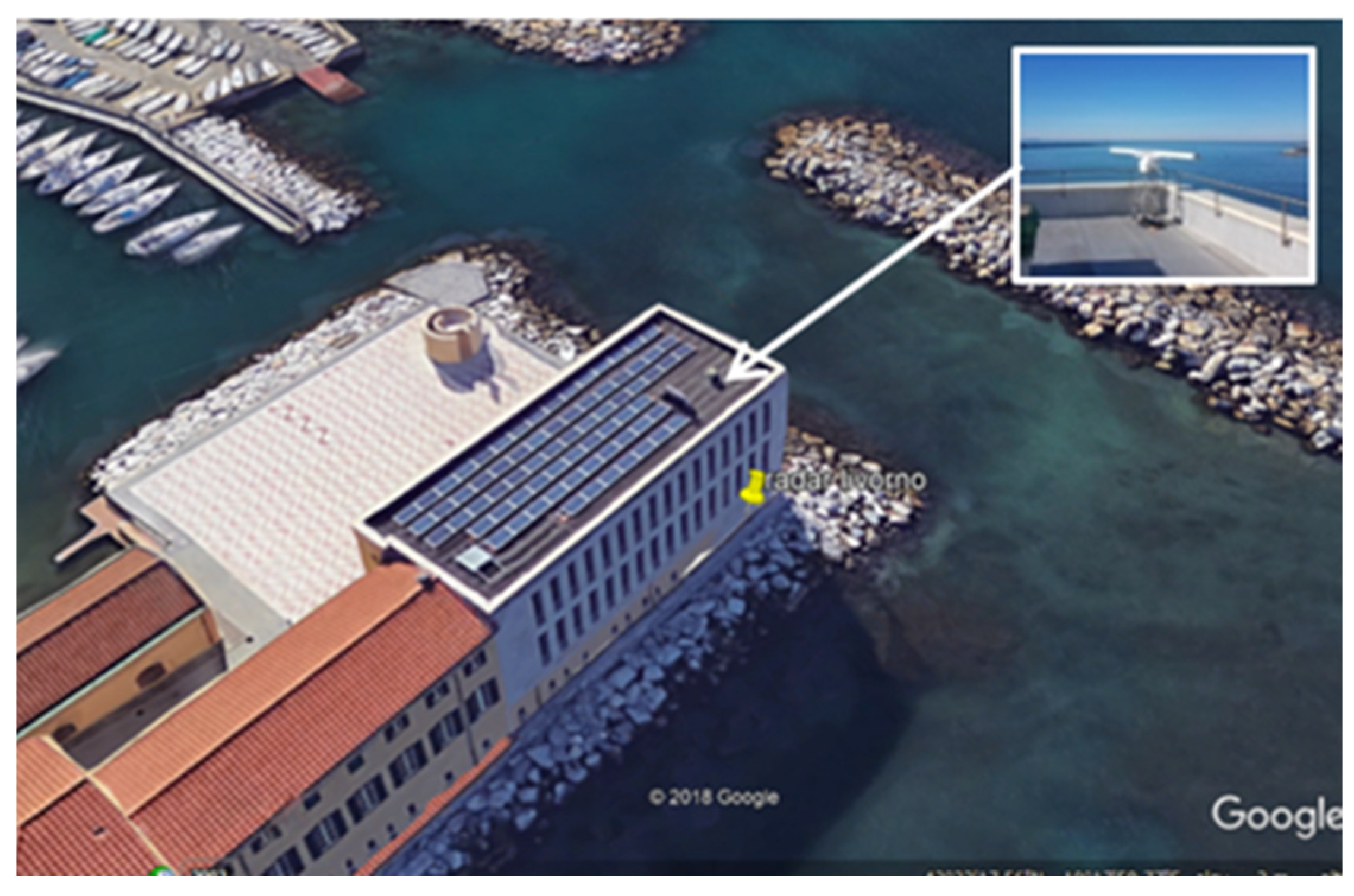
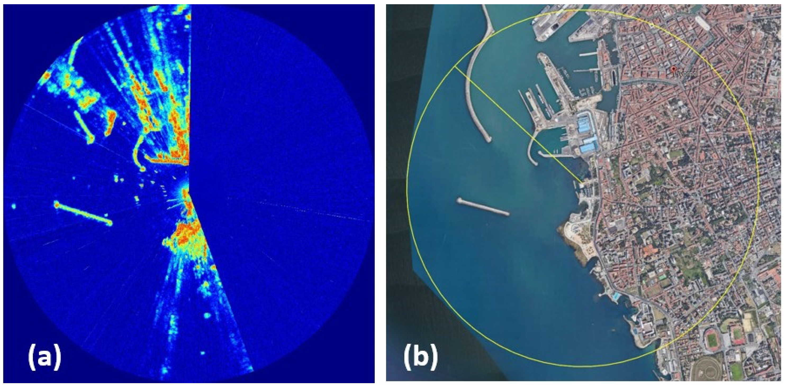
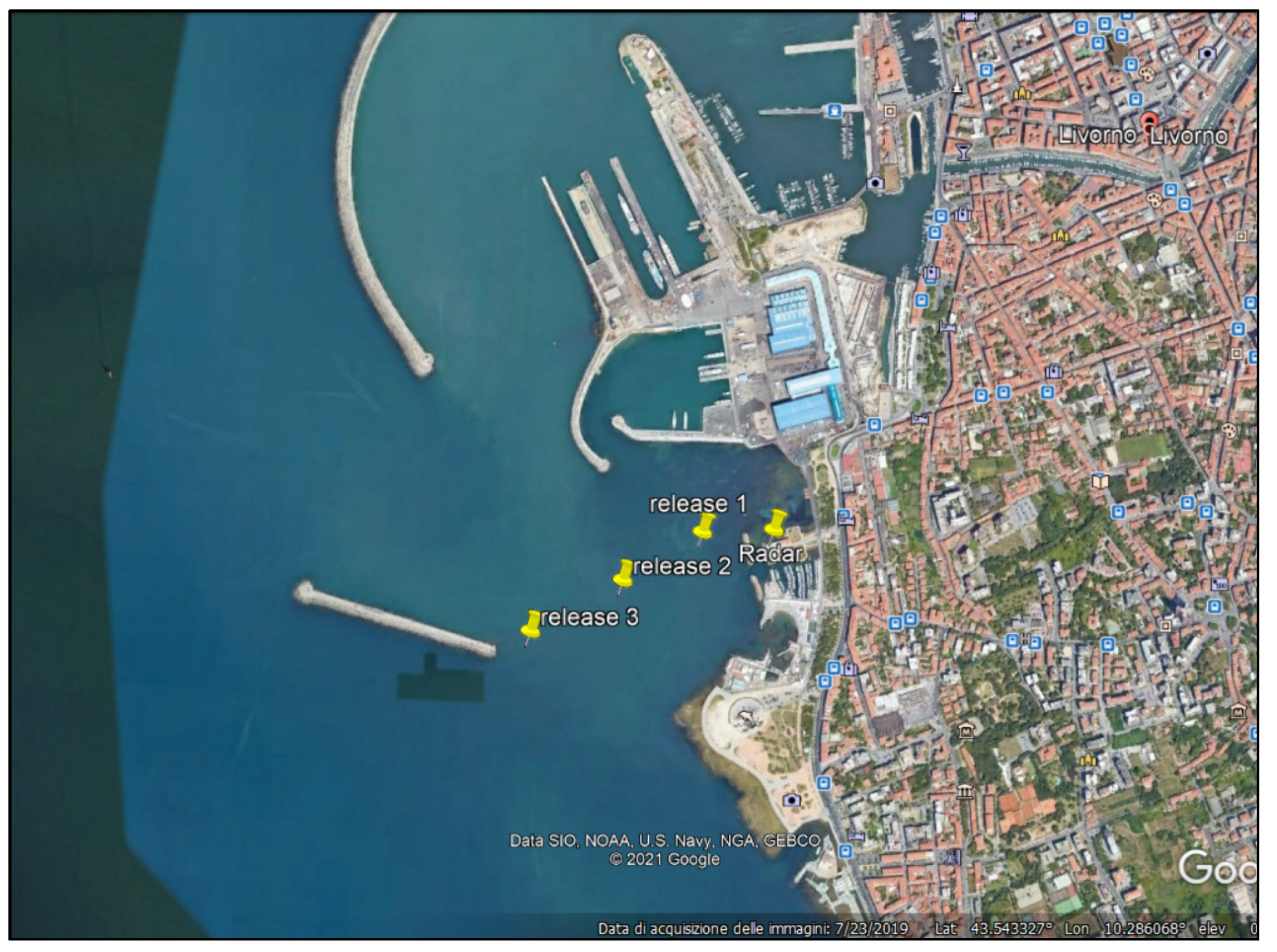
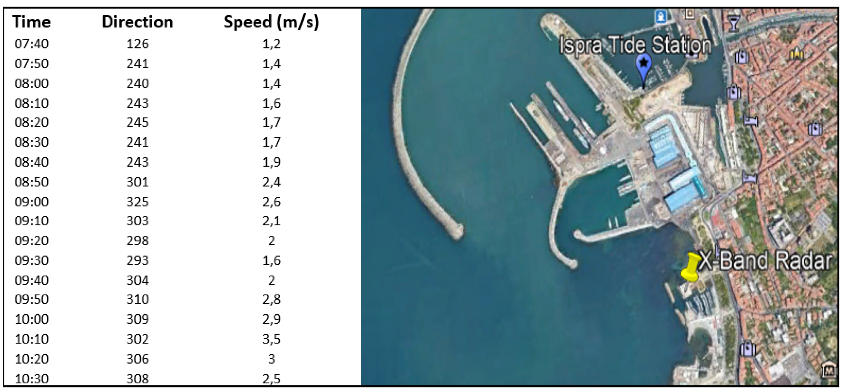
2.2. Description of the Survey Area

The area in which the measurement campaign was conducted is the stretch of sea in front of the south entrance of the port of Livorno, which is where the building called “Scoglio della Regina”, the headquarters of IBE-CNR, is situated. On the roof of the building, an X-band radar, which was purchased with funds from the RITMARE network coordinated by IBE, is installed. The area investigated covers a radius of approximately 0.98 nautical miles. This particular stretch of sea is characterized by the presence of intense maritime traffic as well as several beacons that signal dangers to navigation. From a morphological point of view, it is delimited by the port infrastructures that protect the outer harbor (Molo della Vegliaia and Molo nuovo) and the Azimut Benetti shipyard, and the cliff on which the initial part of Livorno seafront stands (Terrazza Mascagni).

Figure 2 shows a radar image of the area (Figure 2a) and a Google map (Figure 2b) where, as well as the position of the radar, it is possible to see the port infrastructures, the cliff and the signaling beacons. The radar images in this work are a color-scale (from blue to red) spatial representation of the intensity of the signal transmitted by the antenna and reflected by the targets. When a target is highly reflective, the intensity of the reflected signal received by the antenna is greater and, consequently, its color-scale representation tends to red. On the contrary, if a target is less reflective, its color-scale representation tends to green and blue.

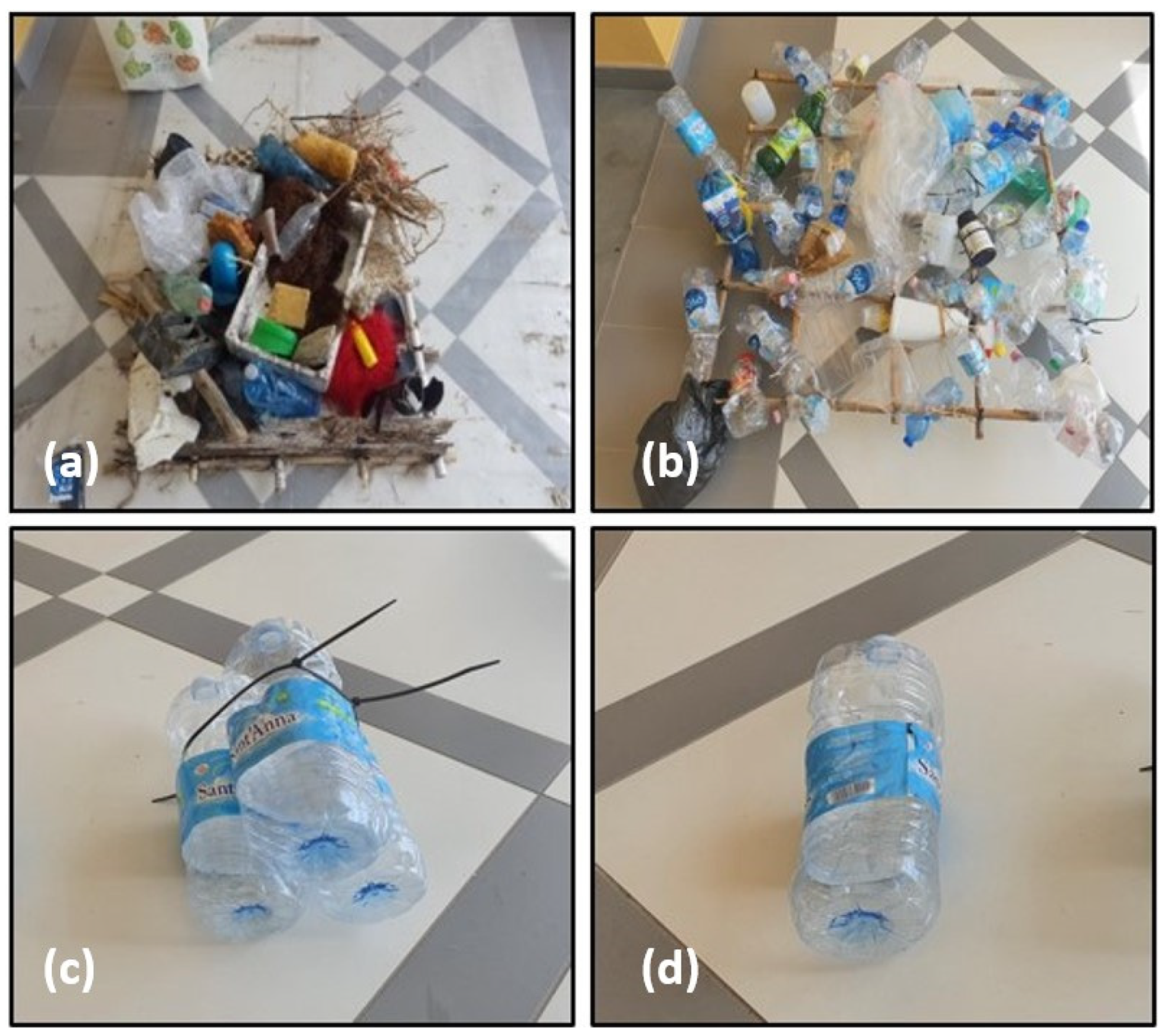
2.3. Small Garbage Island (SGI) Module Construction

To verify the ability of an X-band marine radar to identify and track small islands/aggregations of waste in the sea, it was first necessary to fabricate some SGI modules in the laboratory.

To this aim, waste was collected along the marine coast located immediately north of the port of Livorno. It was decided to collect all the different types of materials found on the beach, i.e., plastic, wood and metal (Figure 3), to assemble a first basic module that could approximate the garbage islands that are formed in the sea by the aggregative effect of winds and currents.

In order to make the measurements repeatable and standardizable, a first basic module with dimensions 1 m × 1 m that could be representative of the garbage aggregations typically found on the sea surface, and that could be used as a reference for the definition of the radar detection capability in terms of resolution and Radar Cross Section (RCS), was created. Using plastic ties, all the objects collected were fixed to a grid with a square base of 1 m × 1 m, which was made using common reeds (Arundo donax) collected along the coast together with the waste.

Table 2. Materials used to assemble the basic SGI module.

Materials Used
N. 5 plastic bottles (three 1.5 L bottles and two 0.5 L bottles)
N. 1 polystyrene box
N. 3 pieces of wood of different sizes
N. 2 women’s shoes
N. 1 aluminum spray can
N. 2 plastic jars
N. 3 different types of fishing net
N. 3 pieces of polyurethane foam
N. 1 plastic wrapping sheet

shows the list of objects used to assemble the first basic module.

Figure 4 shows the sequence of operations carried out to assemble the SGI basic module used for the radar measurements.

In addition to the basic module made using mixed waste, a second SGI module was then fabricated (Figure 5) using only plastic bottles. The second module was assembled using a grid made with the same material (common reeds), same characteristics and dimensions as the one used for the mixed waste module as a rigid base (Figure 5b).

Finally, in order to verify the detection capability of the radar also for smaller-size plastic objects, and check the sensitivity limits of the signal with respect to the targets size, two other modules consisting, respectively, of three plastic bottles tied with a plastic band (Figure 5c) and a single plastic bottle (Figure 5d) were assembled.

The set of modules used as targets for the measurement campaign is shown in Figure 5.

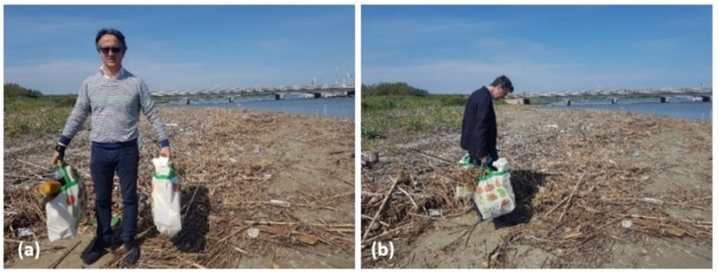
2.4. Measurement Campaign

To evaluate the detection capabilities of the radar and the maximum distance at which it can detect the SGIs, three different releases of the modules described in the previous section were carried out at three different distances from the antenna, as per

Table 3. Release ranges of the SGI modules.

SGI Release Ranges
Release 1	0.12 NM
Release 2	0.24 NM
Release 3	0.39 NM

and as shown in Figure 6.

Releases were carried out at different distances in order to understand the distance limits within which the radar is able to detect the presence of the targets.

To facilitate the reading of the results of the measurement campaign, the experimental modules above were identified as follows:

T0: the target consisting of the basic module made using mixed waste;

T1: the target consisting of the module made solely of plastic;

T2: the target consisting of the module made with the three plastic bottles tied with a plastic band;

T3: the target consisting of the module made with one plastic bottle.

The radar remained switched on for the entire duration of the measurement campaign, recording the raw data, which were subsequently analyzed in the laboratory.

2.5. Radar Data Processing

In this work, to define the radar’s ability to detect small plastic islands, an analysis of the intensity of the radar signal received and reflected by the modules released into the sea was carried out. The experimentation was carried out in calm sea conditions in order to verify the sensitivity of the radar in an ideal scenario. The presence of a high sea state, in fact, reduces the radar’s ability to detect objects on the sea surface. In future developments, analyses will also be carried out in different sea conditions, in order to understand how much the sea state affects the performance of the analysis.

This being a preliminary study, together with the radar data, it was necessary to acquire the photographic images of the study area in order to clearly identify the targets detected by the radar. All this is necessary to understand if it is possible to distinguish the signal coming from plastic waste from that coming from other targets in the radar image. The results obtained in this first phase of the research showed that the characteristics of the signal reflected by small plastic islands is different, and therefore discriminable, from that reflected by other targets (e.g., small boats and buoys, beacons, etc.).

In Figure 7, the radar and photographic images of the survey area of the first release of the targets can be seen. All the targets present in the area, i.e., the targets released (T0, T1, T2, T3), signaling beacons (Buoy 1, Buoy 2, Buoy 3, Buoy 4), boats and port infrastructures are clearly visible. The purpose of this work was to verify the ability of X-band radars to distinguish aggregates of plastic (small garbage islands) and/or mixed waste including plastic from other targets commonly present at sea (boats, beacons, buoys, stretches of coast, metal objects, etc.) and define the evolution of the trajectories followed by the individual targets as a result of the effect of winds and surface currents.

The step-by-step sequence of the radar data analysis procedure used to identify the targets is given below:

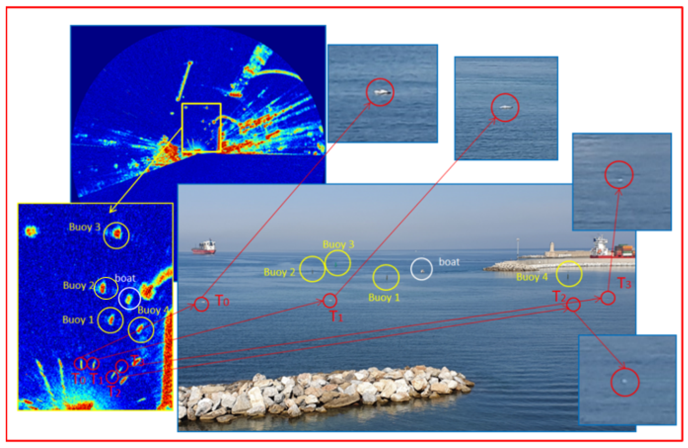
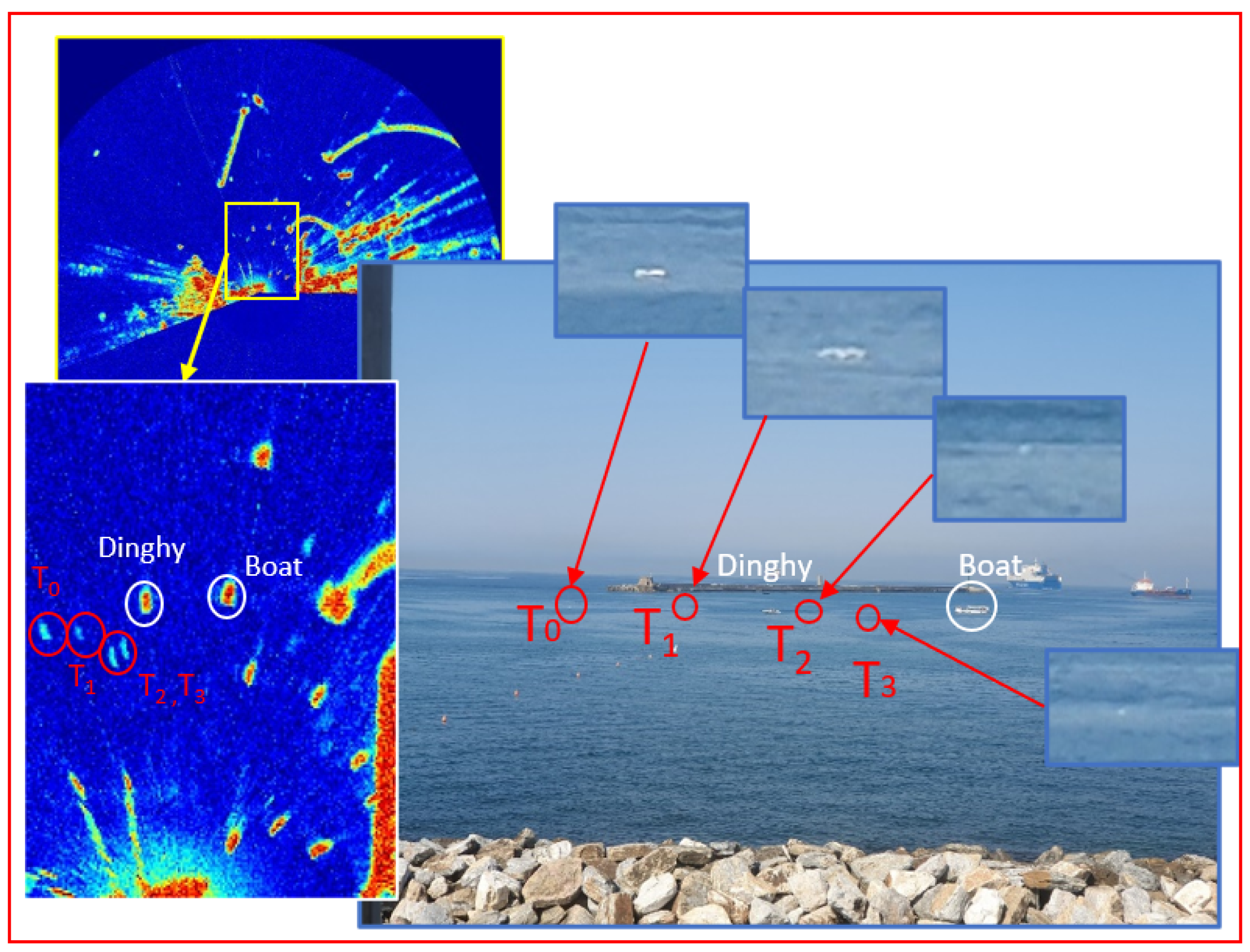
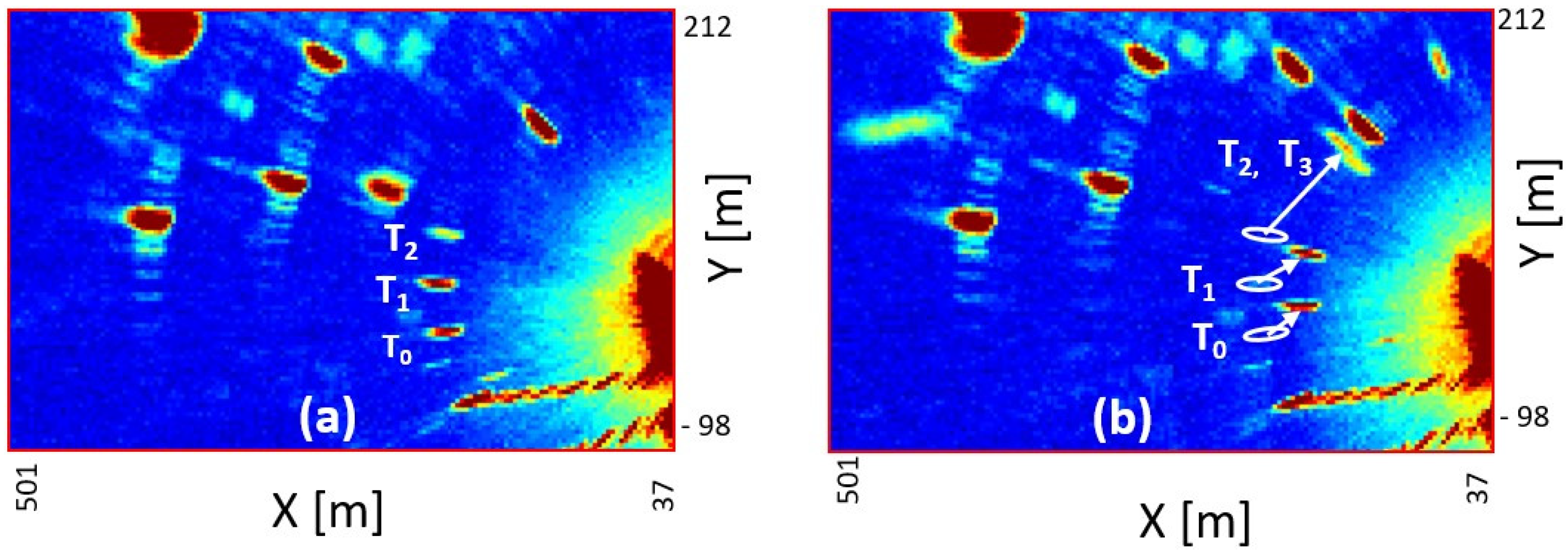
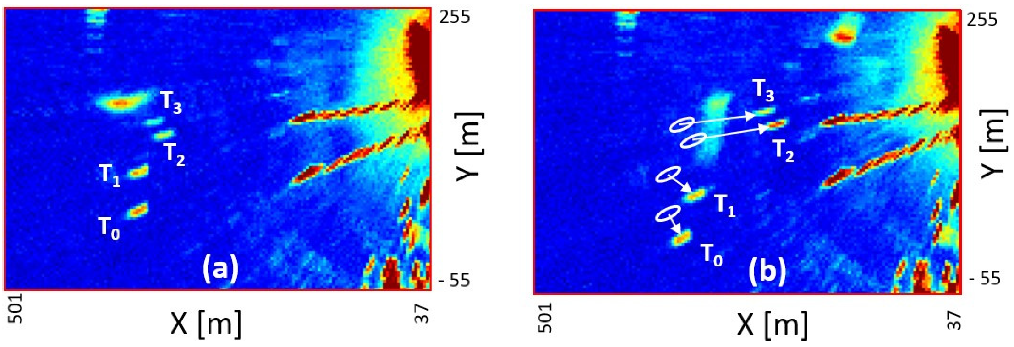
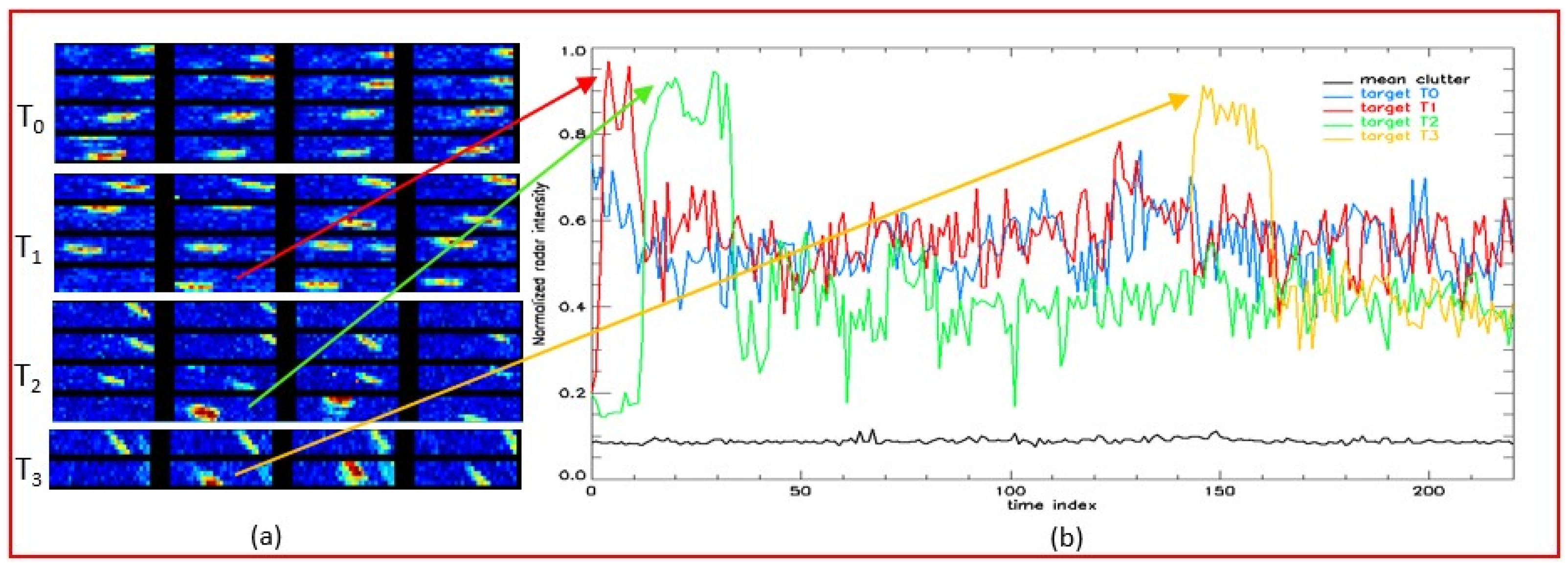
• Identification of the targets on the radar image using photographic images (Figure 7). This phase is essential to have spatial and temporal references to ensure the exact identification of the targets;
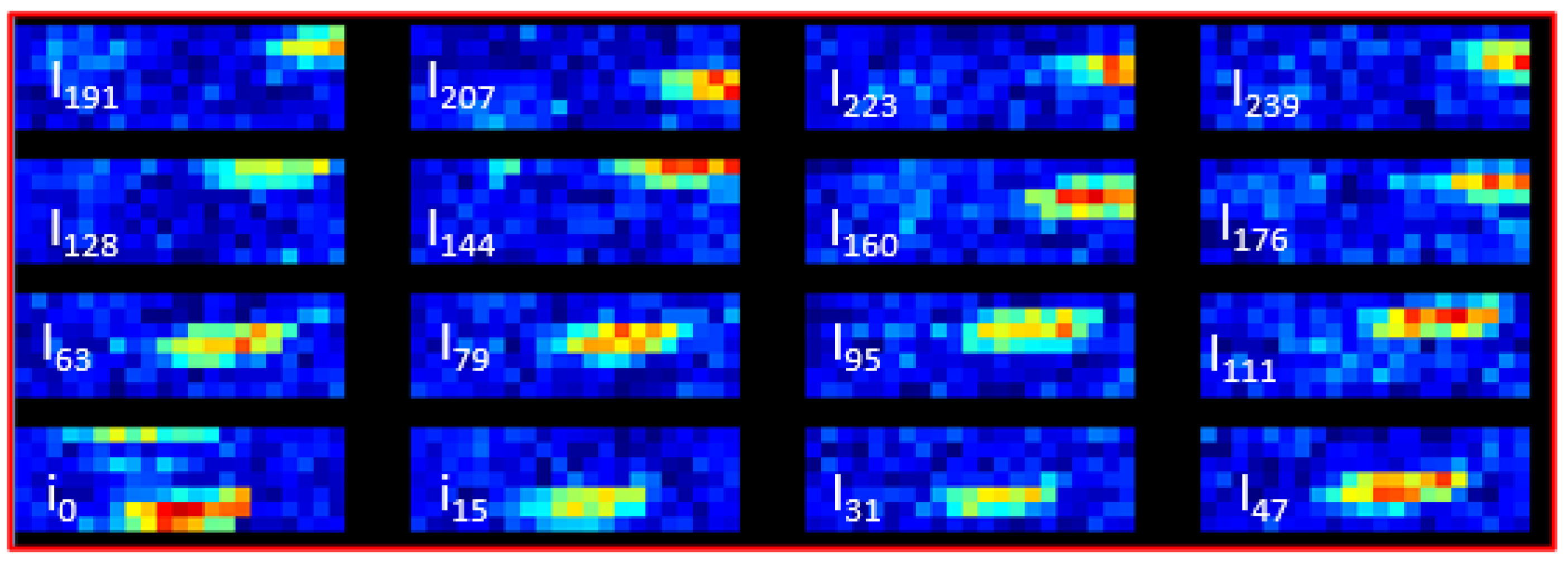
• Extraction of mobile sub-areas containing the targets under investigation for each of the targets T0, T1, T2 and T3. Due to the presence of surface currents and wind, targets are subject to drift/leeway; therefore, it would be necessary to define mobile sub-areas that are able to "follow" the targets while also taking into account their speed. However, in this work, to ensure the presence of the targets within the sub-areas, a manual tracking procedure was adopted, as shown in Figure 8. In a future work, it will be appropriate to define a more accurate and robust procedure for a dynamic definition of the sub-areas, such as to automatically compensate for the drifting of the targets and so that the sub-areas are exactly centered on the targets;
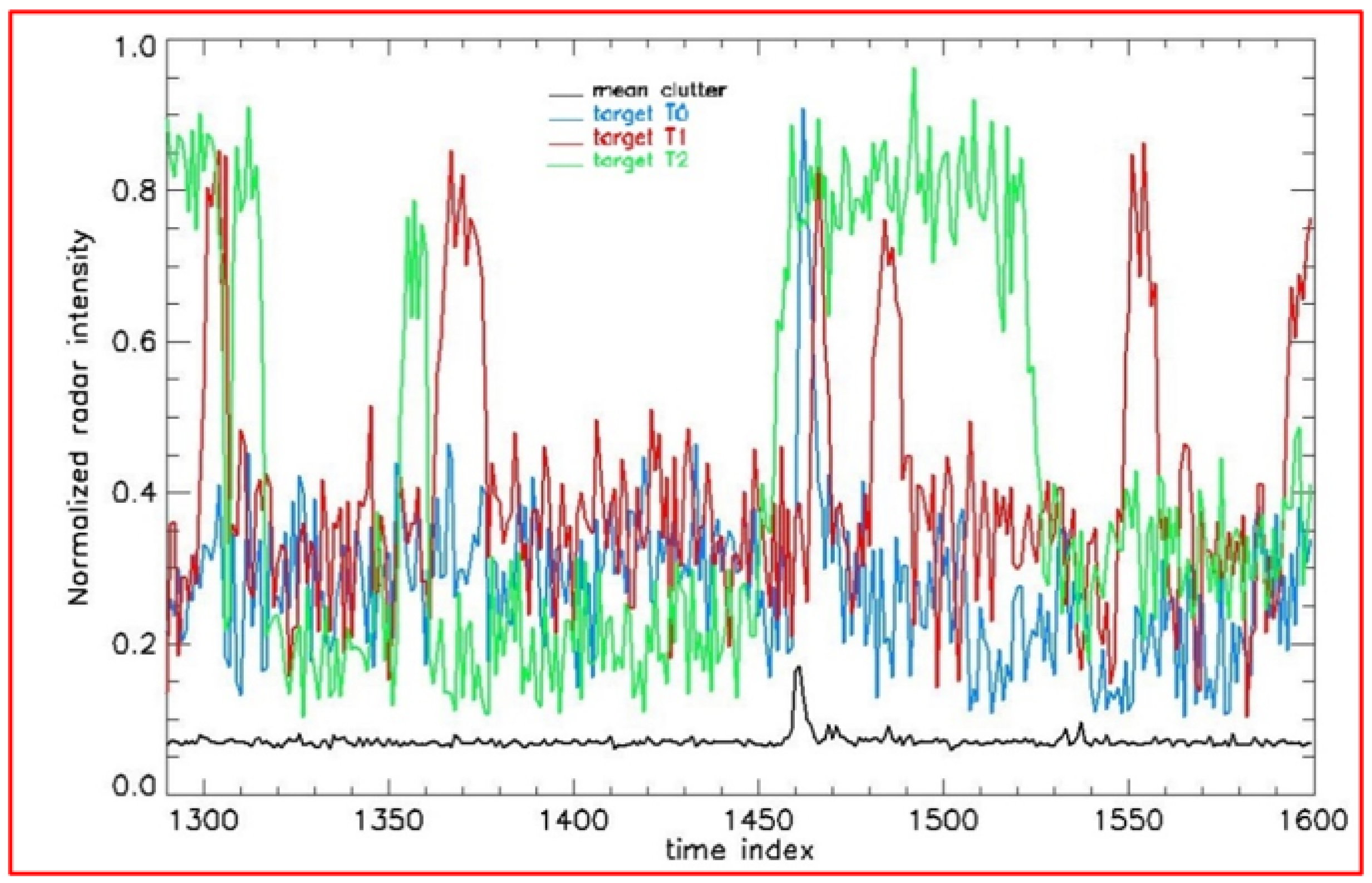
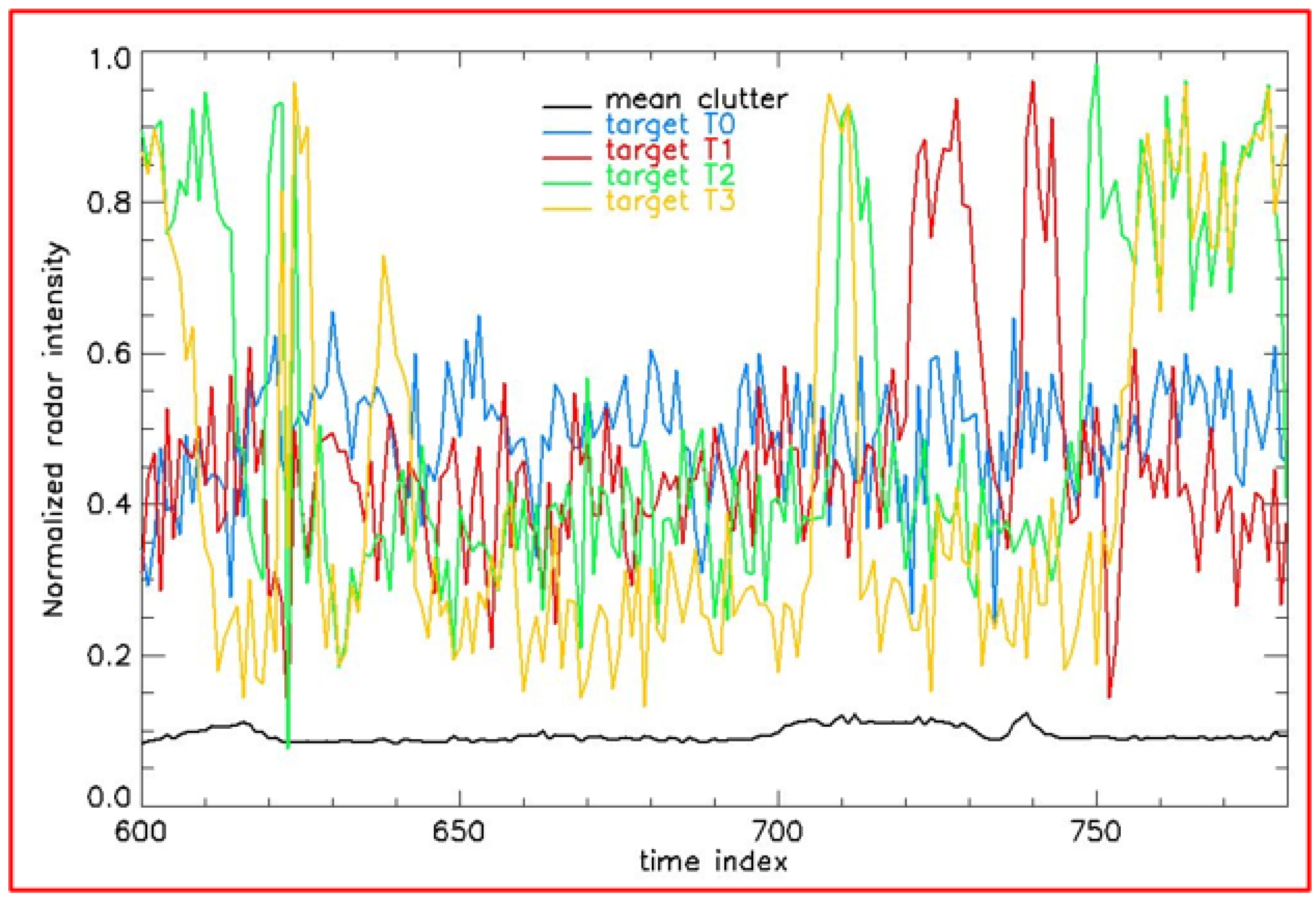
• Measurement of the maximum intensity value detected for each sub-area containing the targets T0, T1, T2 and T3 at each instant of time.

Figure 8 shows the sequence of the sub-areas extracted from the radar images (with an extraction step of a sub-area every 16 instants of time) for target T0. The sequence should be read from bottom to top and from left to right.

3. Results

3.1. Radar Signal Intensity Analysis

Figure 9a shows the set of the sequences of the sub-areas extracted for targets T0, T1, T2, T3, with an extraction step of a sub-area every 16 instants. Figure 9b shows the trend over time of the radar intensities of the individual targets normalized with respect to the maximum radar intensity recorded during the test. The black line at the bottom represents the average value of a sub-area containing only the clutter extracted in the vicinity of the area where the targets were released.

The high intensity values highlighted by the arrows in Figure 9b for the target curves T1 (red line), T2 (green line) and T3 (yellow line) are due to the entry into the sub-area of the inflatable dinghy used for the releases; it follows that these extremely high intensity values are associated with the radar signal of the boat and not with that coming from the targets. Given the high radar reflectivity of the inflatable dinghy, this occurrence was recorded by the radar as a sudden rise (spike) in the radar intensity of the areola containing the targets until the inflatable dinghy left the sub-area. The delay of the yellow line associated with target T3 is due to the fact that T3 was the last target to be released into the sea, at around the 140th instant. Figure 10 shows both the radar and photographic representations of the second release (in the 0.38 NM band). From a first analysis it seems to emerge that the signal coming from the targets is very clear and may be associated with the targets themselves; future analyses could better clarify this aspect as well.

Figure 11 shows the trend over time of the radar intensities of targets T0, T1, T2 and T3 normalized with respect to the maximum radar intensity recorded during the experiment. The black line at the bottom represents the average value of a sub-area containing only the clutter extracted in the vicinity of the area where the targets were released.

Additionally, in this case, the high intensity values highlighted in Figure 11 for the curves of targets T1 (red line), T2 (green line) and T3 (yellow line) are due to the entry into the sub-area of the inflatable dinghy used for the releases. Finally, Figure 12 shows the trend of the radar intensities of the targets related to the third release. Unlike the previous two releases, only targets T0, T1 and T2 are visible, while target T3 was not detectable by the radar.

The high radar intensity values of targets T1 (red line) and T2 (green line) are due to the entry into the sub-areas of the individual targets of the rubber dinghy or other boats present in the field of experimentation.

3.2. Target Shift/Movement Analysis

Further work was carried out on the radar data with the aim to reconstruct the movements of the targets within the survey area. Figure 13 shows two radar images of the stretch of sea used for the experimentation related, respectively, to the beginning of the first release of the targets (Figure 13a) and before their recovery (Figure 13b), where targets T0, T1, T2 and T3 are clearly visible. To facilitate the targets’ displacement visualization, in Figure 13b white arrows have been inserted that join the positions assumed by the targets immediately after release (shown with white circles) with the radar images of the targets before recovery.

Figure 14 shows two radar images of the study area related to the second release. The images were extracted, respectively, at the beginning (Figure 14a) and at the end of the second release (Figure 14b).

In both of the figures, the movements of all the targets can be observed. In particular, targets T0 and T1, which are characterized by a greater weight and surface area, move much more slowly and in different directions compared to targets T2 and T3. Figure 15, instead, shows the radar images of the survey area related to the third release. The images were extracted at three different instants of time (Figure 15a index instant 1320; Figure 15b index instant 1461; Figure 15c index instant 1567). The analysis of the figures makes it possible to understand how, differently from the first two releases, all the targets move following a different trend from the others.

Table 4. Speed and direction of movement of the targets in the survey area.

	Speed T0 and T1 (cm/s)	Speed T2 and T3 (cm/s)	Direction T0 (°)	Direction T1 (°)	Direction T2 and T3 (°)
First release	6	16	45	45	45
Second release	7	17	150	132	80

reports the travel speeds and directions (with respect to the North) followed by target pairs T0 and T1, and T2 and T3 during the first two releases.

Table 5. Speed of movement of targets T0, T1 and T2 during the third release.

	Speed T0 (cm/s)	Speed T1 (cm/s)	Speed T2 (cm/s)	Direction T0 (°)	Direction T1 (°)	Direction T2 (°)
Section 1	5	12	26	90	90	83
Section 2	6	14	33	74	90	98

shows the average speeds of the three targets between instants 1320 and 1461 (Section 1) and between instants 1461 and 1567 (Section 2).

4. Discussion

Before discussing the results of the measurement campaign, it is important to state that the entire experiment took place in the absence of waves and with almost no wind. Figure 16 shows the data related to the evolution of wind direction and speed recorded by the anemometer installed on the ISPRA tidal weather station in Livorno, which is located less than one km from the area where the experiment was conducted. The anemometer measures the direction and intensity of the wind at a height of 10 m above sea level. This section may be divided by subheadings. It should provide a concise and precise description of the experimental results and their interpretation, as well as the experimental conclusions that can be drawn.

Figure 17, instead, shows the trend of the average height of the waves recorded by "Gombo", the wave buoy of the Functional Center of the Tuscany Region, from midnight of 31 July 2020 (day of the measurement campaign) to midnight of 2 August 2020. The buoy is located off the Pisan coast, a few miles from the survey area, and the data recorded can be considered representative of the state of the sea also in the area where the measurement campaign was conducted.

As far as the identification and recognition of the SGI modules is concerned, it is possible to state the following: in relation to the first release, all targets, T0, T1, T2 and T3 (Figure 9), are clearly visible from the radar and can be clearly distinguished from the average sea clutter. In the second release, all the targets are visible, but due to the greater distance from the receiving antenna, the intensity of the radar signal backscattered by the targets is lower compared to that detected during the first release (Figure 12).

By analyzing the movements of the targets, it is possible to observe that both in the first (Figure 13) and in the second release (Figure 14), the pairs of targets T0 and T1 follow a substantially different trend in terms of both direction and speed (Table 4) from that followed by the pair of targets T2 and T3. In particular, as a first approximation, it is possible to state that the trajectories of targets T0 and T1 were not influenced by the very light wind blowing on the sea surface at the time of the experiment and their displacement is substantially due to the surface currents in the area. Similarly, it is possible to state that the displacements of targets T2 and T3 were mainly influenced by the very light wind blowing in the area. All this is due to the greater weight of targets T0 and T1, which made them less subject to the action of very light wind compared to the lighter targets T2 and T3, which consisted, respectively, of three plastic bottles tied together and a single plastic bottle.

During the third release, instead, the displacements of targets T0, T1 and T2 (the only ones visible) followed an even different trend. The joint analysis of Figure 15 and Table 5 makes it possible to understand how the speed of the targets during the experimentation was not uniform, which suggests the presence of a fairly heterogeneous field of surface currents in the survey area.

These latest findings make it possible to identify a possible further development of the potential use of X-band radars also for the purpose of studying surface currents in the absence or in the presence of light wind. In fact, the estimation of the field of surface currents by means of X-band radars requires the presence of wind and rough sea.

5. Conclusions

The purpose of the radar measurement campaign illustrated in this work was to verify the ability of a common nautical X-band radar to detect the presence and track the movements of targets made mainly or exclusively of plastic, and define the limitations of its use in terms of distance from the antenna. In particular, the results of the work have shown that in calm sea conditions, the characteristics of the signal reflected by SGIs is different, and therefore discriminable, from that reflected by other targets; future analyses could better clarify this aspect as well. In any case, further and wider analyses will be useful to verify the results of this preliminary research activity.

Indeed, in calm sea conditions and with almost no wind, the empirical data extrapolated through the analysis procedure defined above have shown that the X-band radar distinguishes the experimentation targets within the maximum distance of 0.39 nautical miles from the receiving antenna. Beyond this distance, the intensity of the signal received by the radar mixes with the average sea clutter.

The results of the measurement campaign also show good potential for the use of X-band radars to estimate the local current regime in the absence of waves and wind. The relatively limited distance of the optimal range of visibility of the radar restricts the possibilities of using X-band radars within fairly limited areas, revealing a potential use of radars for monitoring floating plastic waste at harbor mouths and river mouths, as well as inside the confined zones of protected marine areas. With regard to the radar data analysis procedure used to identify the targets, for the future it will be appropriate to make it more robust, especially as far as the aspects related to the identification of the sub-areas defined in paragraph 2.4 are concerned. In particular, it will be necessary to define an acquisition procedure of the sub-areas that is able to automatically compensate for the drifting of the targets, thus ensuring that the sub-areas are always centered on the targets. Furthermore, it is important to underline that the measurement campaign presented in this report was carried out with a sea state characterized by the absence of waves and almost complete absence of wind, in order to verify the sensitivity of the radar in optimal conditions; it follows that in the future, it will be necessary to conduct further measurement campaigns also in the presence of rough sea (which makes the detection of small targets more difficult), so as to evaluate the radar system performance as the sea conditions vary, and identify the sea state threshold limit beyond which the intensity of the backscattered signal mixes with the average sea clutter, making the use of the radar ineffective. A further possible future development could be to repeat the experiments by releasing into the sea SGI modules made of different materials and also of larger dimensions, in order to characterize the system for a wider range of materials and scenarios.

References

1. Beaumont, N.J.; Aanesen, M.; Austen, M.C.; Borger, T.; Clark, J.R.; Cole, M.; Hooper, T.; Lindeque, P.K.; Pascoe, C.; Wyles, K.J. Global ecological, social and economic impacts of marine plastic. Mar. Pollut. Bull. 2019, 142, 189–195. [Google Scholar] [CrossRef]
2. Derraik, J.G.B. The pollution of the marine environment by plastic debris: A review. Mar. Pollut. Bull. 2002, 44, 842–852. [Google Scholar] [CrossRef]
3. Sheavly, S.B.; Register, K.M. Marine debris & plastics: Environmental concerns, sources, impacts and solutions. J. Polym. Environ. 2007, 15, 301–305. [Google Scholar]
4. Barnes, D.K.A.; Galgani, F.; Thompson, R.C.; Barlaz, M. Accumulation and fragmentation of plastic debris in global environments. Philos. Trans. R. Soc. Lond. B Biol. Sci. 2009, 364, 1985–1998. [Google Scholar] [CrossRef] [Green Version]
5. Thompson, R.C.; Moore, C.; Vom Saal, F.S.; Swan, S.H. Plastics, the environment and human health: Current consensus and future trends. Philos. Trans. R. Soc. B 2009, 364, 2153–2166. [Google Scholar] [CrossRef] [PubMed]
6. Law, K.L.; Moret-Ferguson, S.; Maximenko, N.A.; Proskurowsk, G.; Peacock, E.E.; Hafner, J.; Reddy, C.M. Plastic accumulation in the north atlantic subtropical gyre. Science 2010, 329, 1185–1188. [Google Scholar] [CrossRef] [PubMed] [Green Version]
7. UNEP Year Book 2014. Emerging Issues Update. Chapter 8: Plastic Debris in the Ocean. Available online: https://wedocs.unep.org/20.500.11822/9240 (accessed on 3 September 2021).
8. Cozar, A.; Echevarría, F.; González-Gordillo, J.I.; Duarte, C.M. Plastic debris in the open ocean. Procs. Natl. Acad. Sci. USA 2014, 111, 10239–10244. [Google Scholar] [CrossRef] [PubMed] [Green Version]
9. Geyer, R.; Jambeck, J.R.; Law, K.L. Production, use, and fate of all plastics ever made. Sci. Adv. 2017, 3, e1700782. [Google Scholar] [CrossRef] [Green Version]
10. Jambeck, J.R.; Geyer, R.; Wilcox, C.; Siegler, T.R.; Perryman, M.; Andrady, A.; Narayan, R.; Jambeck, K.L.L. Plastic waste inputs from land into the ocean. Science 2015, 347, 768–771. [Google Scholar] [CrossRef]
11. Andrady, A.L. Microplastic in the marine environment. Mar. Pollut. Bull. 2011, 62, 1596–1605. [Google Scholar] [CrossRef]
12. Deudero, S.; Alomar, C. Mediterranean marine biodiversity under threat: Reviewing influence of marine litter on species. Mar. Pollut. Bull. 2015, 98, 58–68. [Google Scholar] [CrossRef] [PubMed]
13. Obbard, R.W.; Sadri, S.; Wong, Y.Q.; Khitun, A.A.; Baker, I.; Thompson, R.C. Global warming releases microplastic legacy frozen in Arctic Sea ice. Earth’s Future 2014, 2, 315–320. [Google Scholar] [CrossRef]
14. Galgani, F.; Barnes, D.K.A.; Deudero, S.; Fossi, M.C.; Ghiglione, J.F.; Hema, T. Executive summary. In CIESM Workshop Monograph 46: Marine Litter in the Mediterranean and Black Seas; Briand, F., Ed.; CIESM Publisher: Monaco, 2014; pp. 7–20. [Google Scholar]
15. Galgani, F. Distribution, composition and abundance of marine litter in the Mediterranean and black seas. In CIESM Workshop Monograph 46: Marine Litter in the Mediterranean and Black Seas; Briand, F., Ed.; CIESM Publisher: Monaco, 2014; pp. 23–30. [Google Scholar]
16. Suaria, G.; Aliani, S. Floating debris in the Mediterranean Sea. Mar. Pollut. Bull. 2014, 86, 494–504. [Google Scholar] [CrossRef]
17. Bertrand, J.; Souplet, L.A.; Gil de Soula, G.; Relini, C.P. International Bottom Trawl Survey in the Mediterranean (Medits), Instruction Manual, Version 5. 2007. Available online: https://www.sibm.it/SITO%20MEDITS/file.doc/Medits-Handbook_V5-2007.pdf (accessed on 3 September 2021).
18. Cheshire, A.C.; Adler, E.; Barbière, J.; Cohen, Y.; Evans, S.; Jarayabhand, S.; Jeftic, L.; Jung, R.T.; Kinsey, S.; Kusui, E.T.; et al. UNEP/IOC Guidelines on Survey and Monitoring of Marine Litter; United Nations Environment Programme: Nairobi, Kenya, 2009; Available online: https://www.researchgate.net/publication/256186638_UNEPIOC_Guidelines_on_Survey_and_Monitoring_of_Marine_Litter (accessed on 3 September 2021).
19. Oosterbaan, L.; Pereira, M.A.; Sheavly, S.; Tkalin, A.; Varadarajan, S.; Wenneker, B.; Westphalen, G. UNEP/IOC Guidelines on Survey and Monitoring of Marine Litter; United Nations Environment Programme: Nairobi, Kenya, 2009. [Google Scholar]
20. Arthur, C.; Murphy, P.; Opfer, S.; Morishige, C. Bringing together the marine debris community using “ships of opportunity” and a Federal marine debris information clearinghouse. In Proceedings of the Fifth International Marine Debris Conference, Honolulu, HI, USA, 20–25 March 2011; pp. 449–453. [Google Scholar]
21. Van Franeker, J.A.; Blaize, C.; Danielsen, J.; Fairclough, K.; Gollan, J.; Guse, N.; Hansen, P.L.; Heubeck, M.; Jensen, J.K.; Le Guillou, G.; et al. Monitoring plastic ingestion by the northern fulmar Fulmarus glacialis in the North Sea. Environ. Poll. 2011, 159, 2609–2615. [Google Scholar] [CrossRef] [PubMed]
22. Hidalgo-Ruz, V.; Gutow, L.; Thompson, R.C.; Thiel, M. Microplastics in the marine environment: A review of the methods used for identification and quantification. Environ. Sci. Techn. 2012, 46, 3060–3075. [Google Scholar] [CrossRef]
23. Imhof, H.K.; Schmid, J.; Niessner, R.; Ivleva, N.P.; Laforsch, C. A novel, highly efficient method for the separation and quantification of plastic particles in sediments of aquatic environments. Limnol. Oceanogr.-Methods 2012, 10, 524–537. [Google Scholar] [CrossRef]
24. Claessens, M.; Van Cauwenberghe, L.; Vandegehuchte, M.B.; Janssen, C.R. New techniques for the detection of microplastics in sediments and field collected organisms. Mar. Pollut. Bull. 2013, 70, 227–233. [Google Scholar] [CrossRef]
25. Galgani, F.; Hanke, G.; Werner, S.; Oosterbaan, L.; Nilsson, P.; Fleet, D.; Kinsey, S.; Thompson, R.C.; Van Franeker, J.; Vlachogianni, T.; et al. Guidance on Monitoring of Marine Litter in European Seas, Eur-Scientific and Technical Research Series 2013. Available online: https://mcc.jrc.ec.europa.eu/documents/201702074014.pdf (accessed on 3 September 2021).
26. Galgani, F.; Hanke, G.; Werner, S.; De Vrees, L. Marine litter within the European Marine Strategy. ICES J. Mar. Sci. 2013, 70, 1055–1064. [Google Scholar] [CrossRef]
27. Ryan, P.G. A simple technique for counting marine debris at sea reveals steep litter gradients between the straits of Malacca and the bay of bengal. Mar. Pollut. Bull. 2013, 60, 128–136. [Google Scholar] [CrossRef]
28. Maximenko, N.; Arvesen, J.; Asner, G.; Carlton, J.; Castrence, M.; Centurioni, L.; Chao, Y.; Chapman, J.; Chirayath, V.; Corradi, P.; et al. Remote sensing of marine debris to study dynamics, balances and trends. In Community White Paper Produced at the Workshop on Mission Concepts for Marine Debris Sensing; International Pacific Research Center: Honolulu, HI, USA, 2016. [Google Scholar]
29. Hafeez, S.; Wong, M.S.; Abbas, S.; Kwok, C.Y.T.; Nichol, J.; Ho Lee, K.; Tang, D.; Pun, L. Detection and monitoring of marine pollution using remote sensing technologies. In Monitoring of Marine Pollution; Fouzia, H.B., Ed.; Intech. Open: London, UK, 2019; p. 568. [Google Scholar]
30. Moy, K.; Neilson, B.; Chung, A.; Meadows, A.; Castrence, M.; Ambagis, S.; Davidson, K. Mapping coastal marine debris using aerial imagery and spatial analysis. Mar. Pollut. Bull. 2018, 132, 52–59. [Google Scholar] [CrossRef]
31. Maximenko, N.; Corradi, P.; Law, K.L.; Van Sebille, E.; Garaba, S.P.; Lampitt, R.S.; Galgani, F.; Martinez-Vicente, V.; Goddijn-Murphy, L.; Veiga, J.M.; et al. Toward the integrated marine debris observing system. Front. Mar. Sci. 2018, 6, 447. [Google Scholar] [CrossRef] [Green Version]
32. Lauren, B.; Daniel, C.; Victor, M.; Topouzelis, V.; Topouzelis, K. Finding plastic patches in coastal waters using optical satellite data. Sci. Rep. Nat. Res. 2020, 10, 5364. [Google Scholar]
33. Maximenko, N.; Jan Hafner, J.; Niiler, P. Pathways of marine debris derived from trajectories of Lagrangian drifters. Mar. Pollut. Bull. 2012, 65, 51–62. [Google Scholar] [CrossRef]
34. Zambianchi, E.; Trani, M.; Falco, P. Lagrangian transport of marine litter in the mediterranean sea. Front. Environ. Sci. 2017, 5, 5. [Google Scholar] [CrossRef] [Green Version]
35. Nieto Borge, J.C.; Guedes Soares, C. Analysis of directional wave fields using X-band navigation radar. Coast. Eng. 2000, 40, 375–391. [Google Scholar] [CrossRef]
36. Nieto Borge, J.C.; Rodríguez, G.R.; Hessner, K.; Gonzáles, P.I. Inversion of marine radar images for surface wave analysis. J. Atmos. Ocean. Technol. 2004, 21, 1291–1300. [Google Scholar] [CrossRef]
37. Senet, C.M.; Seemann, J.; Flampouris, S.; Ziemer, F. Determination of bathymetric and current maps by the method DiSC based on the analysis of nautical X-Band radar image sequences of the sea surface. IEEE Trans. Geosci. Remote Sens. 2008, 46, 2267–2279. [Google Scholar] [CrossRef]
38. Serafino, F.; Lugni, C.; Soldovieri, F. A novel strategy for the surface current determination from marine X-band radar data. IEEE Geosci. Remote Sens. Lett. 2010, 7, 231–235. [Google Scholar] [CrossRef]
39. Serafino, F.; Lugni, C.; Nieto Borge, J.C.; Zamparelli, V.; Soldovieri, F. Bathymetry determination via X-band radar data: A new strategy and numerical results. Sensors 2010, 10, 6522–6534. [Google Scholar] [CrossRef]
40. Serafino, F.; Lugni, C.; Ludeno, G.; Arturi, D.; Uttieri, M.; Buonocore, B.; Zambianchi, E.; Budillon, G.; Soldovieri, F. REMOCEAN: A flexible X-band radar system for sea-state monitoring and surface current estimation. IEEE Geosci. Remote Sens. Lett. 2012, 9, 822–826. [Google Scholar] [CrossRef]
41. Ludeno, G.; Brandini, C.; Lugni, C.; Arturi, D.; Natale, A.; Soldovieri, F.; Gozzini, B.; Serafino, F. Remocean system for the detection of the reflected waves from the costa Concordia ship wreck. IEEE J. Sel. Top. Appl. Earth Obs. Remote Sens. 2014, 7, 3011–3018. [Google Scholar] [CrossRef]
42. Gwee, R.; Bushman, F. Detecting floating plastic using a high-frequency X-band Radar. Deltares 2020. Available online: https://publications.deltares.nl/11205287_018.pdf (accessed on 3 September 2021).
Figure 1. Photo of the Scoglio della Regina building with the detail of the radar.
Remotesensing 13 03558 g001
Figure 2. (a) Radar image of the survey area; (b) aerial image of the survey area (Google, images ©2019 CNES).
Remotesensing 13 03558 g002
Figure 3. CNR (a) and ISPRA (b) researchers engaged in the collection of the waste.
Remotesensing 13 03558 g003
Figure 4. Assembly phases of the basic SGI module.
Remotesensing 13 03558 g004
Figure 5. Set of modules used as targets in the measurement campaign. (a) Target T0; (b) Target T1; (c) Target T2; (d) Target T3.
Remotesensing 13 03558 g005
Figure 6. Map with the locations of the releases of the SGI modules (Google, images ©2019 CNES).
Remotesensing 13 03558 g006
Figure 7. Radar and photographic representations of the first release of the targets.
Remotesensing 13 03558 g007
Figure 8. Sequence of the sub-areas of target T0 extracted with a frequency of one every sixteen instants of time.
Remotesensing 13 03558 g008
Figure 9. (a) Sequence of the sub-areas containing the targets; (b) trend of the radar intensities of the targets.
Remotesensing 13 03558 g009
Figure 10. Radar and photographic representations of the second release of the targets.
Remotesensing 13 03558 g010
Figure 11. Radar intensities of the targets related to the second release.
Remotesensing 13 03558 g011
Figure 12. Radar intensities of the targets related to the third release.
Remotesensing 13 03558 g012
Figure 13. Movements of the targets within the study area related to the first release. (a) Beginning of the first release of the target; (b) before recovery of the target.
Remotesensing 13 03558 g013
Figure 14. Movements of the targets within the survey area related to the second release. (a) Beginning of the second release of the target; (b) before recovery of the target.
Remotesensing 13 03558 g014
Figure 15. Movements of the targets within the survey area related to the third release. (a) Index instant 1320; (b) index instant 1461; (c) index instant 1567.
Remotesensing 13 03558 g015
Figure 16. Wind direction and speed measured by the ISPRA tidal weather station in the port of Livorno.
Remotesensing 13 03558 g016
Figure 17. Wave height recorded by “Gombo”, the wave buoy of the Functional Center of the Tuscany Region.
Remotesensing 13 03558 g017