Article

Fusing Measurements from Wi-Fi Emission-Based and Passive Radar Sensors for Short-Range Surveillance

Department of Information Engineering, Electronics and Telecommunications, Sapienza University of Rome, 00184 Rome, Italy
*
Author to whom correspondence should be addressed.
Remote Sens. 2021, 13(18), 3556; https://doi.org/10.3390/rs13183556
Submission received: 2 July 2021 / Revised: 6 August 2021 / Accepted: 8 August 2021 / Published: 7 September 2021
(This article belongs to the Special Issue Radar Signal Processing for Target Tracking)

Abstract

:
In this work, we consider the joint use of different passive sensors for the localization and tracking of human targets and small drones at short ranges, based on the parasitic exploitation of Wi-Fi signals. Two different sensors are considered in this paper: (i) Passive Bistatic Radar (PBR) that exploits the Wi-Fi Access Point (AP) as an illuminator of opportunity to perform uncooperative target detection and localization and (ii) Passive Source Location (PSL) that uses radio frequency (RF) transmissions from the target to passively localize it, assuming that it is equipped with Wi-Fi devices. First, we show that these techniques have complementary characteristics with respect to the considered surveillance applications that typically include targets with highly variable motion parameters. Therefore, an appropriate sensor fusion strategy is proposed, based on a modified version of the Interacting Multiple Model (IMM) tracking algorithm, in order to benefit from the information diversity provided by the two sensors. The performance of the proposed strategy is evaluated against both simulated and experimental data and compared to the performance of the single sensors. The results confirm that the joint exploitation of the considered sensors based on the proposed strategy largely improves the positioning accuracy, target motion recognition capability and continuity in target tracking.

1. Introduction

The detection, localization, tracking and classification of threats at short ranges have become the key requirements for surveillance systems intending to protect critical infrastructures, as well as private premises from intruders or hostile incursions, with an emphasis on unmanned aerial vehicles (UAV) [1,2,3,4]. To this purpose, different sensing technologies might be employed, including audio, video, infrared (IR), radio frequency (RF) and radar sensors, a combination of two or more technologies being a preferable solution for improving the system performance and increasing its reliability.
Among the technologies mentioned, sensors exploiting microwave signals at convenient frequency bands play an important role, since they guarantee a 24-h all-weather monitoring capability; they can provide decent coverage, operating with small-sized antennas, and they are not subject to the blind spots and potentially intrusive equipment required by video surveillance. With particular reference to the scenario at hand, passive sensors based on existing RF sources are especially attractive, since no extra signal is transmitted, and this limits the energy consumption, prevents possible interference with pre-existing systems and makes the sensor inherently covert and free from any restriction on its installation in populated areas and/or any other site where electromagnetic emissions are limited by regulations in force.
In light of the above reasons, and building onto the recent results obtained by the authors [5,6], in this paper, we consider the joint exploitation of passive sensors based on Wi-Fi transmissions, i.e., signals of the IEEE 802.11 Standard in a 2.4-GHz band [7]. Specifically, we focus on two different sensors that implement alternative approaches to the passive exploitation of Wi-Fi signals: (i) the Wi-Fi-based Passive Bistatic Radar (PBR) and (ii) the Wi-Fi emission-based technique or Passive Source Location (PSL). The concept of the two techniques is sketched in Figure 1.
A PBR sensor exploits the Wi-Fi Access Point (AP) as an illuminator of opportunity and detects moving objects by receiving and properly processing the signals backscattered by the targets [8,9,10,11,12]. Target localization is then based on the Angle of Arrival (AoA) and/or bistatic range measurements of the detected echoes.
The PSL technique relies on the fact that the target of interest is equipped with an active device emitting signals in the Wi-Fi band (e.g., a smartphone carried by a human subject or a wireless module in a remotely piloted aircraft). In fact, PSL sensors detect the radiation emitted by the device and estimate the source position based on its AoA and Time Difference of Arrival (TDoA) measurements [5,6].
In references [5,6], the Wi-Fi-based PSL and PBR approaches have been preliminary investigated and compared in the considered surveillance scenario, and their suitability and complementarity have been demonstrated for the detection and localization of people and drones at short ranges. However, the unpredictable and complex motions of the targets of interest, typically showing “move-stop-move” patterns, make their continuous tracking a challenging task for each of the two techniques.
Therefore, in this paper, the joint exploitation of the above sensors is considered, and an effective measurement fusion strategy is proposed in order to benefit from the diversity of the information conveyed by the two different approaches. Specifically, our efforts are devoted to the case where the target to be tracked has a move-stop-move motion pattern and the sources of measurement are intermittent, which is quite typical for the short-range surveillance applications with the Wi-Fi-based passive sensors considered in this study. In fact, it is known that the PBR measurements are only available for moving targets, and also, the PSL sensor might experience a decrease in the number of available measurements, depending on the global traffic load and user behavior [5,6]. We leverage the above characteristics to introduce appropriate modifications to the conventional techniques in order to tackle the challenge of tracking human being and commercial UAVs.
To this purpose, we resorted to an ad hoc multi-sensor version of the Interacting Multiple Model (IMM) tracking algorithm employing data fusion techniques [13,14,15,16]. The proposed algorithm exploits the knowledge of the characteristics of the specific sensors providing measurements to properly modify the innovation process. In turn, this improves their capability to select the best-suited motion model among those interacting within the IMM scheme. The proposed strategy is firstly tested against simulated data in order to understand its performance in controlled scenarios by varying the relevant parameters. Then, the results of the multi-sensor experimental tests are reported to prove the effectiveness of the proposed approach against real-world scenarios, including both human targets and small commercial drones.
This paper is organized as follows. In Section 2 the two employed Wi-Fi-based sensors are briefly described, together with a possible receiver setup and the signal processing techniques required to detect and localize the target. The sensor fusion strategy is presented in Section 3, and its performance is analyzed against simulated and experimental data in Section 4 and Section 5, respectively. Finally, in Section 6, we draw our conclusions.

2. Wi-Fi-Based Sensor Description

Since the two sensing techniques exploit the same signals, we first illustrate the multi-channel receiver architecture considered in this paper, which effectively accommodates both the sensors. Then, we briefly recall the principles of operation and the signal processing techniques required by the PBR and the PSL approaches, respectively. Finally, their expected performances and inherent characteristics are comparatively discussed, as this provides the basic motivation for their joint exploitation.

2.1. Multichannel Receiver Architecture and System Setup

Different implementations could be considered for each of the sensing techniques by varying the number of parallel receiving channels offered by the employed hardware.
Aiming at a simple and effective solution, we assume that the sensors are implemented using a single four-channel receiver commonly available among commercial-off-the-shelf (COTS) software-defined radios (SDR). Moreover, since the same signals of opportunity are exploited with the two techniques, the same receiver can be adopted to implement both the approaches if a suitable arrangement of receiving nodes can be identified.
In the following, in order to guarantee a 2D localization capability with both approaches using the minimum number of receiving nodes, a double node system is considered, with Rx nodes A and B appropriately displaced to cover a wide surveillance area but connected to the same SDR (see Figure 1). Specifically, we assume node A to always be equipped with a pair of closely spaced antennas to enable the estimation of the AoA. In contrast, the number of surveillance antennas available at node B might be either one or two, depending on the strategy adopted to collect the signal emitted by the AP. In fact, as will be detailed later, in order to guarantee an effective operation of the PBR approach, a good copy of the signal emitted by the Wi-Fi AP should be made available at the receiver, namely the reference signal.
In the considered short-range applications, there are two different ways to obtain a clean reference waveform [8,9]:
(1)
If the transmitter of opportunity is directly accessible, and it is possible to introduce a directional coupler between the AP and its antenna, a solution is to connect it to one of the channels of the four-channel Rx. It is worth mentioning that, whilst providing quite a good copy of the signal of opportunity, this approach requires a dedicated receiving channel to be used to collect the reference signal. We explicitly note that, in this case, with the considered setup, the overall system can feature up to three surveillance channels so that node B will employ a single antenna when receiving.
(2)
If the Wi-Fi router is not accessible, then the reference waveform must be extracted from the signal collected by one of the surveillance antennas. Specifically, the transmitted signal can be reconstructed by demodulating and remodulating the received signal according to the IEEE 802.11 standard. This approach may suffer from the reconstruction errors, but it avoids the need for a dedicated reference channel. In this case, with the considered hardware setup, it is possible to implement a double-node system where both nodes are equipped with an interferometric pair of surveillance antennas to enable the estimation of the AoA.
For illustration purposes, the sketch in Figure 1 encompasses both strategies, as they will be alternatively adopted in the experimental results reported in this paper.

2.2. Passive Bistatic Radar

A Wi-Fi-based passive radar parasitically exploits the signals emitted by a Wi-Fi AP to detect and localize moving targets based on their backscattering. The geometry is inherently bistatic, the AP and the passive receiver usually located in different positions (see Figure 1).
Despite the Wi-Fi signal being of a pulsed type, the short-range operation implies a direct signal from the AP, its multipath replicas and the Doppler-shifted echoes from potential targets to be simultaneously received by the sensor. Consequently, appropriate signal-processing techniques are required to extract the weak target echo from the competing background and to estimate its position.
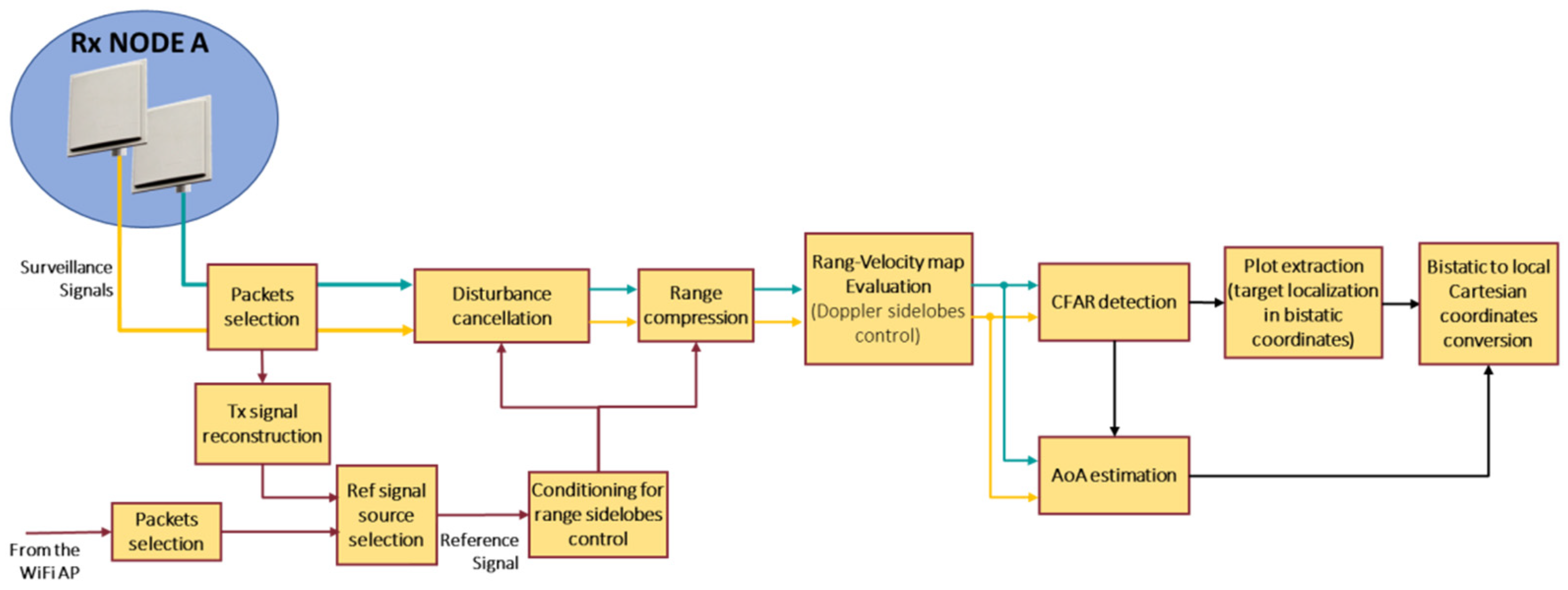
The typical signal processing chain is sketched in Figure 2 for a Rx node employing two surveillance antennas [8,9].
First of all, the signal fragments corresponding to Wi-Fi packets emitted by the AP are identified and extracted from the received data stream based on the source MAC address. When the transmitted waveform is not directly acquired from the AP, the reconstruction of the transmitted waveform from the surveillance channels should also be performed at this stage. Hence, the subsequent stages are independent of the reference signal source selection.
The processing scheme must typically include the clutter/multipath cancellation stage for the disturbance removal. Different approaches could be employed to implement this stage. In particular, the sliding version of the Extensive Cancellation Algorithm (ECA-S) has been shown especially effective when aiming at mitigating the effect of the returns from the stationary scene while slowly preserving the moving target echoes [17]. It operates by subtracting from the surveillance signals properly scaled and delayed versions of the reference signal. As a direct consequence of this processing stage, the direct signal breakthrough and multipaths are effectively cancelled, together with the echoes from stationary targets.
Then, a range compression stage is implemented by cross-correlating the surveillance signals and the reference signal on a pulse-by-pulse basis. Subsequently, the obtained results are coherently integrated over a set of consecutive packets. In fact, the range of compressed pulses included in the selected coherent processing interval (CPI) undergoes an FFT stage in order to obtain the bistatic range Doppler map. Proper techniques for the range and Doppler sidelobes control are applied, since the Ambiguity Function (AF) of the Wi-Fi signals is characterized by high sidelobes in both the range and Doppler dimensions [8].
After the main processing stages described above, a clutter-cancelled range–velocity map is obtained at each surveillance channel. A CFAR threshold is separately applied to each of the two channels, and a decentralized strategy is exploited to combine the detections, i.e., target detection is declared only for targets that exceed the threshold at both the surveillance channels. The subsequent plot extraction provides a first target localization over the bistatic range–velocity plane. In addition, by measuring the phase difference of the target echo on the two maps, its AoA can be estimated according to a simple interferometric approach.
Target localization in local Cartesian coordinates is finally obtained by finding the intersection of the ellipse corresponding to the bistatic range measurement and a line corresponding to the AoA measurement. Consequently, we observed that the single node A of the considered system setup (Figure 1) is sufficient for the PBR approach to provide target localization on the x-y plane.
In principle, the measurements obtained at the two nodes might be combined to increase the localization accuracy of the resulting multi-static sensor [9]. However, this approach requires an effective plot association to be implemented, which is not a straightforward task in dense scenarios. In fact, the targets are observed under different bistatic geometries at the different nodes, which makes the measurement-to-target association more challenging if multiple targets are present. Therefore, in the following study, we assume that the target localization provided by the PBR technique is obtained based on node A of the system setup, i.e., always equipped with two antennas when receiving. This approach also allows to effectively implement the measurement-to-target association stage in the native bistatic range/Doppler domain of the PBR sensor, where the finer velocity resolution yields an increased capability to discriminate among the measurements belonging to different targets. The analyses reported in reference [9] have shown that a positioning accuracy in the order of a few meters could be obtained with this approach for the typical values of the signal-to-noise ratio (SNR) at short ranges.

2.3. Passive Source Location

The PSL detects the presence of a target by detecting the signals emitted by the Wi-Fi devices carried by the target, e.g., mobile devices, smartphones and Wi-Fi transponders of remotely piloted objects. As a consequence, with this approach, only specific classes of targets are covered. Once the target has been detected, its position is estimated by properly combining the measurements provided by multiple receiving nodes.
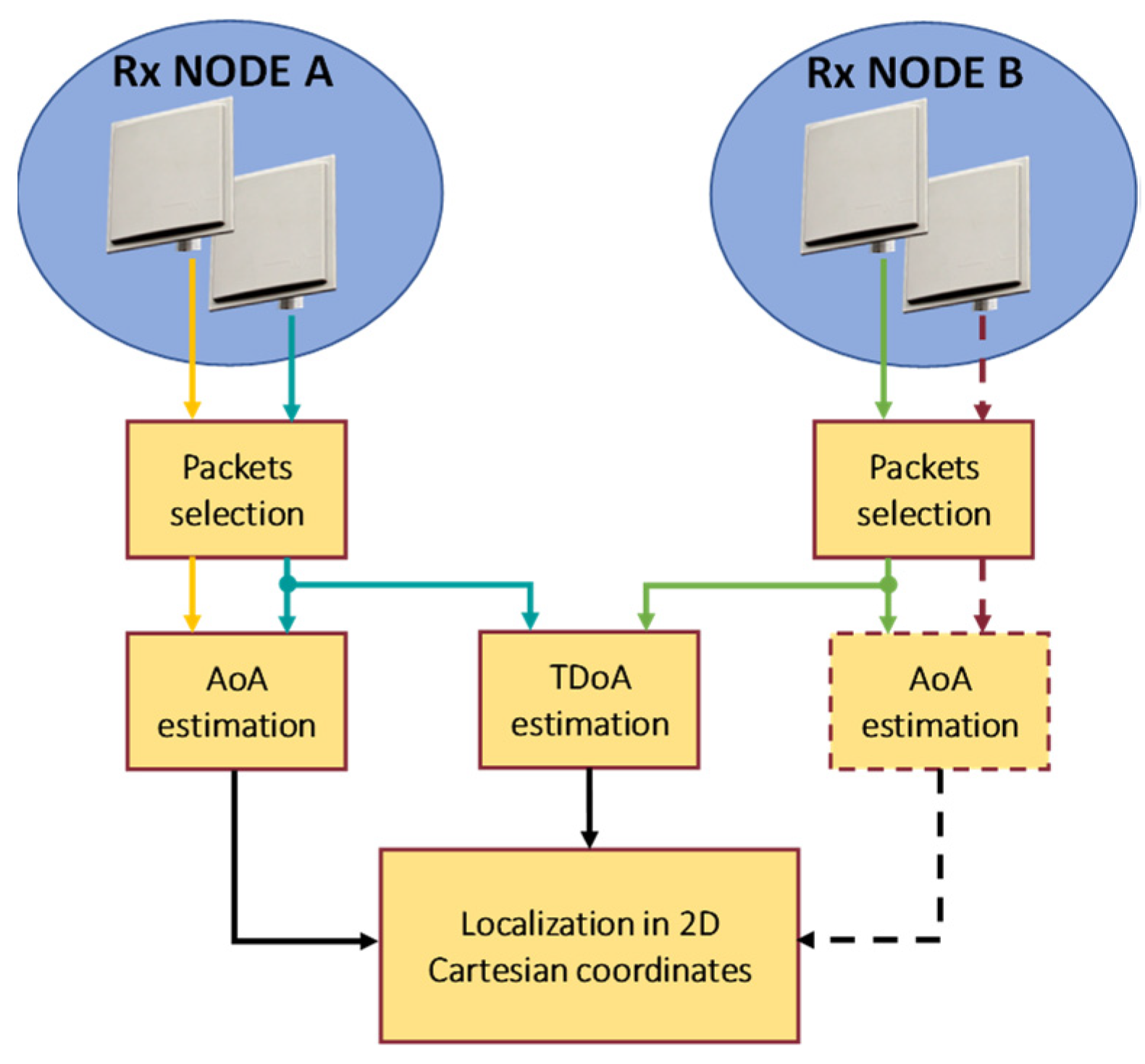
With reference to the dual-node setup considered in this paper, the foreseen processing scheme is sketched in Figure 3.
First of all, the Wi-Fi packets are detected at each Rx channel, and the packets emitted by a specific device are extracted from the received data stream based on the source MAC address. It is worth observing that this approach inherently solves the measurements-to-target association problem even in a dense target scenario. By measuring the interferometric phase difference of a given signal fragment as received by two closely spaced antenna elements, its AoA can be estimated. With the system at hand, this possibility is certainly enabled by node A.
An additional AoA estimate is provided by node B only when strategy #2 is adopted to collect the reference signal to be exploited by the PBR (see Section 2.1). In such a case, the two AoA measurements are sufficient to provide the final target localization in 2D cartesian coordinates. This is easily obtained by finding the intersection of the corresponding lines in the plane.
In contrast, when strategy #1 is adopted to collect the reference signal for the PBR, node B only features one surveillance antenna. In such a case, target 2D localization can still be obtained by estimating the TDoA of the selected packets at the two nodes. This basically provides the second equation, i.e., a hyperbola, to be used together with the line equation provided by the AoA from node A, to evaluate the unknown x-y coordinates.
The analyses reported in references [5,6] have shown that the positioning accuracy obtained with this approach largely varies with the packet transmission rate of the considered device, as well as with the instantaneous geometry. As for the PBR case, positioning errors in the order of a few meters could be obtained under favorable conditions.

2.4. Complementarity of PBR and PSL

Based on their principles of operation and signal processing techniques, the PBR and PSL clearly show complementary aspects that make them appealing for joint exploitations [5]. Such aspects are briefly summarized in Table 1 and discussed in the following section.
First of all, by comparing Figure 2 and Figure 3, we observe that the PSL technique is characterized by a lower complexity for the required signal processing scheme, which, in turn, requires a lower computational load. In fact, the higher SNR conditions of the direct signals transmitted by the target provide the possibility to avoid all the steps required by the PBR for the extraction of the weak target echoes.
It is worth mentioning that the device-based strategy is effective even against closely spaced targets, since their signals are discriminated against based on the MAC address of the emitting device; in contrast, the PBR cannot discriminate targets moving on similar trajectories due to the limited range Doppler resolution brought on by the Wi-Fi signals.
Moreover, the device-based strategy allows the detection and localization of stationary targets, whereas the PBR cannot detect their presence or estimate their position, because their echoes are cancelled by the clutter cancellation stage. On the other hand, the PSL might be inaccurate for moving targets, especially if the measurements extraction is averaged over multiple consecutive Wi-Fi packets; additionally, we observe that the packet transmission rate might decrease when the user is moving.
PBR is an essential tool when the target does not carry a Wi-Fi active device or its signal transmission is disabled, as is typically the case in surveillance applications.
Eventually, we recall that the performances of the PBR and the PSL techniques are strictly linked to the number of Wi-Fi packets transmitted by the AP and the target device, respectively [5]. Due to the Time Division Multiple Access (TDMA) approach used in the Wi-Fi Standard [7], the devices and AP cannot transmit simultaneously, which, in some cases, might result in a lack of measurements from one of the two sensors. Therefore, the joint exploitation of the two considered approaches has the inherent potential to compensate for the lack of measurements due to intensive Wi-Fi channel usage.

3. Sensor Fusion for Target Localization

In this section, we present a new methodology for jointly exploiting the observations provided by the PBR and PSL sensors for improved short-range surveillance applications.
The obvious objective of the proposed approach is to enhance the target detection and localization accuracy of the resulting passive system that leverages the fusion of the measurements performed by the two individual sensors. In addition, the complementary characteristics of the employed sensors have the potential to increase the reliability of the system, as well as to widen its range of uses.
Since a peculiar characteristic of the targets of interest is their switch between move and stop conditions, we also aimed to exploit the inherent differences between the PBR and the PSL sensors to improve the tracking capability of the move-stop-move targets typically encountered in the considered scenarios. To this purpose, we observe that we are using two sensors whose performances are directly connected to the target motion status. Even more, their differences are emphasized when the target alternates the motion and stationary intervals along its path. In fact, the PSL has been shown to yield a reduced continuity of operations against moving objects, whereas the PBR sensor is unable to detect and localize stationary targets. As a consequence, even a lack of measurements might provide information about the target’s motion status if properly interpreted.
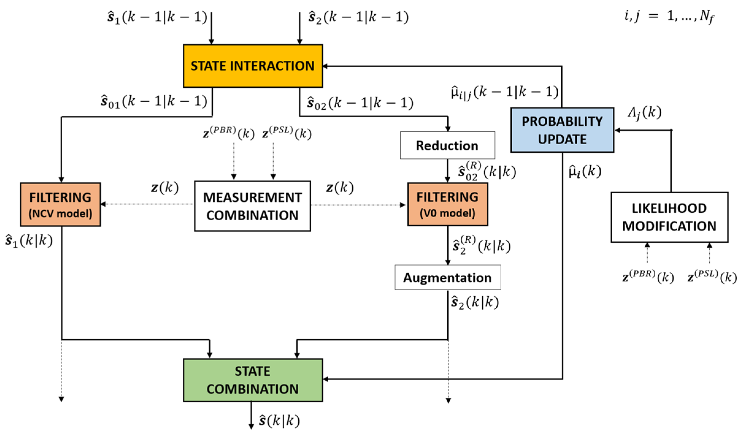
To this aim, we propose a new strategy that uses a modified version of the IMM approach, together with data fusion techniques. The high-level schematic diagram of the proposed strategy is reported in Figure 4. As apparent, it exploits a conventional IMM scheme with two interacting tracking filters respectively dedicated to the motion and stop conditions. The basic idea of the proposed method is to exploit the presence or the absence of the PBR measurements to drive the choice of the best-suited motion model among those interacting within the IMM scheme. This is obtained via an appropriate factitious modification of the innovation process. Therefore, we will refer to the proposed approach as the Interacting Multiple Model–Modified Innovation (IMM-MI).
In the following Section, we will briefly recall the conventional multi-sensor IMM method [18], as it represents the basis of the proposed scheme. The proposed modification is illustrated in Section 3.2, along with the inherent parameter settings.

3.1. PBR and PSL-Based Interacting Multiple Model Filter

We considered a 2D localization problem. Correspondingly, the target state to be tracked is defined as
s ( k ) = [ x ( k ) x ˙ ( k ) y ( k ) y ˙ ( k ) ] T
where x ( k ) , y ( k ) are the coordinates of the target at time k , while x ˙ ( k ) , y ˙ ( k ) are the velocity components along the x and y axes.
As shown in Figure 4, the basic structure of the proposed approach is that of an IMM with two interacting tracking filters [13,19]. Specifically, the first filter exploits a Nearly Constant Velocity (NCV) motion model that can be described by the following motion equations in a matrix form:
s 1 ( k + 1 ) = Φ 1 s 1 ( k ) + d 1 ( k )
where s 1 ( k ) shares a similar definition as s ( k ) in (1),
d 1 ( k ) = G 1 a ( k )   with   a ( k ) = [ a x ( k ) , a y ( k ) ] T ,
and the following matrices are used:
Φ 1 = [ 1   0   0   0   T   1   0   0   0   0   1   0   0 0 T 1 ] ,     G 1 = [ T 2 / 2 T 0 0   0   0   T 2 / 2 T ]
T being the elapsed time between consecutive updates. Moreover, we indicate with Σ a = E { a ( k ) a T ( k ) } = d i a g { [ σ a x 2   σ a y 2 ] } the covariance matrix of the model errors defined by the acceleration a ( k ) and, with Q 1 = G 1 Σ a G 1 T , the covariance matrix of d 1 ( k ) .
The second filter exploits a stationary (V0) model:
s 2 ( R ) ( k + 1 ) = Φ 2   s 2 ( R ) ( k ) + d 2 ( k )
where the state vector s 2 ( R ) ( k ) is a two-dimensional vector, since it does not include the velocity components (the apex (R) is used as a reminder that this is a reduced version),
d 2 ( k ) = G 2 v ( k )   with   v ( k ) = [ v x ( k )     v y ( k ) ] T ,
and the relevant matrices are defined as follows:
Φ 2 = [ 1 0 0 1 ] ,   G 2 = [ T 0 0 T ]
Moreover, we indicate with Σ v = E { v ( k ) v T ( k ) } = d i a g { [ σ v x 2   σ v y 2 ] } the covariance matrix of the model errors defined by the velocity v ( k ) and, with Q 2 = G 2 Σ v G 2 T , the covariance matrix of d 2 ( k ) .
If a coherent integration of consecutive packets is carried out for both sensors and the same update time is used for them, the PBR and the PSL sensors perform synchronous estimates of the target position. Therefore, if the target is correctly detected by both sensors at time k, two two-dimensional vectors are made available: z ( PBR ) ( k ) and z ( PSL ) ( k ) . They are related to the target state vector via the following expression:
z ( P B R ) ( k ) = H   s ( k ) + w ( P B R ) ( k ) z ( P S L ) ( k ) = H   s ( k ) + w ( P S L ) ( k ) ,
where H represents the incidence matrix, defined as
H = [ 1 0 0 0 0 0 1 0 ]
and the measurements errors, w ( PBR ) ( k ) and w ( PSL ) ( k ) , are statistically independent zero-mean Gaussian random vectors with covariance matrices:
R ( PBR ) ( k ) = [ σ x ( P B R ) 2 ( k ) 0 0 σ y ( P B R ) 2 ( k ) ] R ( PSL ) ( k ) = [ σ x ( P S L ) 2 ( k ) 0 0 σ y ( P S L ) 2 ( k ) ]
where σ x ( P B R ) 2 ( k ) , σ y ( P B R ) 2 ( k ) ,   σ x ( P S L ) 2 ( k ) and σ y ( P S L ) 2 ( k ) are the variances of the measurement errors along the x and y axes provided by the two sensors at time k.
At each time, the scheme in Figure 4:
(i)
combines the sensors measurements into a 2 N s × 1 vector that can be expressed as
z ( k ) = H N s ( k )   s ( k ) + w ( k ) ,
where H N s ( k ) = 1 N s ( k ) × 1 H , N s ( k ) is the number of sensors that provide a measurement at time k ( N s ( k ) = 0, 1 or 2 in our case). When N s ( k )   = 2, we have
z ( k ) = [ z ( PBR ) ( k ) z ( PSL ) ( k ) ] ,
and the error covariance matrix is
R ( k ) = E { w ( k ) w T ( k ) } = [ R ( PBR ) ( k ) 0 0 R ( PSL ) ( k ) ]
(ii)
The combined measurement feeds the two Kalman Filters (KF), based on the NCV and the V0 model. The filter outputs ( s ^ 1 ( k | k ) and s ^ 2 ( R ) ( k | k ) ) represent the current filtered estimates of the target state s ( k ) separately provided by the two filters. Notice that the V0 model has a state space of lower dimensions; therefore, its operations inside the IMM require appropriate stages of state augmentation and reduction in order to convert the 2 × 1 vector s ^ 2 ( R ) ( k | k ) into a 4 × 1 augmented vector s ^ 2 ( k | k ) and vice versa.
(iii)
The outputs of the two filters are combined in the state combination block in order to provide the final IMM filtered state at time k,   s ^ ( k | k ) , using as weights the mode probabilities μ ^ i provided by the probability update block.
(iv)
Eventually, to obtain the required input state for the two filters in the following iterations, the IMM includes a state interaction block that takes as the input the filtered states obtained in the previous iterations: s ^ 1 ( k 1 | k 1 ) and s ^ 2 ( k 1 | k 1 ) and produces two mixed states: s ^ 01 ( k 1 | k 1 ) and s ^ 02 ( k 1 | k 1 ) . These are obtained by a linear combination of the contributions of each filter, using as coefficients the mixing probabilities μ ^ i | j calculated in the probability update stage. Similarly, the related state covariance matrices are obtained as inputs to the two filters by mixing the covariance matrices evaluated in each individual KF.
The operations performed at each stage are summarized in Table 2.

3.2. Innovation Modification and Probability Update

The IMM filter above represents a viable solution for the fusion of the PBR and PSL sensor measurements in the short-range surveillance application. Its use shows a significant improvement of the localization accuracy when both set of measurements are available, whereas a single sensor’s accuracy is retained when one of the two sets of measurements is missing.
To further improve the localization accuracy, with respect to this fusion approach, we propose an appropriate modification that capitalizes on the peculiarities of the considered sensors. In particular, while the lack of measurements for the sensors cannot be recovered, we observe that it conveys information on the target motion status that is not exploited by the IMM filter above.
In fact, the PBR cannot detect stationary objects, so the absence of PBR measurements implies a high probability that the target dynamics follow the V0 model. In contrast, the presence of PBR measurements indicates that the NCV model must be preferred. In addition to this main point, it might be argued that, during the motion state, a person would not stimulate significant use of the Wi-Fi upload channel that is used for the PSL measurements, so the frequency of the PSL detections is expected to be lower. This could further encourage preferring the NCV target model when PBR measurements are available and PSL measurements are missing.
Based on the considerations above, we introduced the information related to the absence of PBR or PSL measurements inside the Probability Update block. As summarized in Table 2, this block evaluates the mode probabilities and the mixing probabilities, which are used in the Combination and Interaction stages, respectively:
μ j ( k ) = Λ j ( k ) c ¯ j Λ 1 ( k ) c ¯ 1 + Λ 2 ( k ) c ¯ 2
and
μ i | j ( k 1 | k 1 ) = 1 c ¯ j p i j μ i ( k 1 )
where
c ¯ j = p 1 j μ 1 ( k 1 ) + p 2 j μ 2 ( k 1 )
p i j being the Markov transition probabilities between the two interacting models, i.e., NCV and V0, and
Λ j ( k ) = 1 | 2 π S j ( k ) | · e x p { 1 2 r j T ( k ) S j 1 ( k ) r j ( k ) }
is the Likelihood of the jth model that represents the capability of that specific model to predict the target behavior.
The proposed modification of the Update Probability Block is implemented by unbalancing the Likelihood function, as detailed in the following section.

3.2.1. Absence of PBR Detections

In the standard IMM filter above, the absence of PBR measurements is handled by simply neglecting the corresponding measurement components. Therefore, assuming that the PSL measurement is available, the innovation vectors of the two filters, exploited in Equation (17), are given by
r 1 ( k ) = z ( PSL ) ( k ) H   s ^ 1 ( k | k 1 ) r 2 ( k ) = z ( PSL ) ( k ) s ^ 2 ( R ) ( k | k 1 )
and the 2 × 2 matrix S j ( k ) is
S 1 ( k ) = H   P 1 ( k | k 1 ) H T + R ( PSL ) ( k ) S 2 ( k ) = P 2 ( R ) ( k | k 1 ) + R ( PSL ) ( k )
To modify this Likelihood, we also included the PBR components of the innovation vectors missing in Equation (18), and we filled them with artificial values. These artificial values were different for the two filters in order to unbalance the Likelihood towards the selection of the V0 model. Specifically, the innovation of the PBR for the V0 filter was set to zero, in order to instruct the system to consider the correct V0 filter output state. In contrast, the innovation of the PBR for the NCV filter was set artificially to a rather high value to encourage the Likelihood to realize that the NCV filter output state was not the correct one.
Specifically, since the absence of the measurements could be due to a value of the detection probability, Pd < 1, we set the innovation equal to a number α times the standard deviation of the measurements. The value of α is set to 1 the first time that the PBR time is missing, while it is set to 2 if there have been at least two consecutive absences of the PBR measurements. Two consecutive absences of the measurements are considered to provide a high probability that we did not just miss the detection due to a low SNR but a lack of detections due to a target stop condition.
The resulting vectors for the two filters are:
r ¯ 1 ( k ) = [ [ α   σ x ( P B R ) ( k ) ,   α   σ y ( P B R ) ( k ) ] T z ( PSL ) ( k ) H   s ^ 1 ( k | k 1 ) ] r ¯ 2 ( k ) = [ 0 2 x 1 z ( PSL ) ( k ) s ^ 2 ( R ) ( k | k 1 ) ]
Correspondingly, the Likelihood function is evaluated as
Λ j ( k ) = 1 | 2 π S j ( k ) | · e x p { 1 2 r ¯ j T ( k ) S ¯ j 1 ( k ) r ¯ j ( k ) }
where the innovation covariance matrices are the 4 × 4 matrices
S ¯ 1 ( k ) = [ H H ] P 1 ( k | k 1 ) [ H H ] T + [ R ( PBR ) ( k ) 0 0 R ( PSL ) ( k ) ] S ¯ 2 ( k ) = [ I 2 × 2 I 2 × 2 ] P 2 ( R ) ( k | k 1 ) [ I 2 × 2 I 2 × 2 ] T + [ R ( PBR ) ( k ) 0 0 R ( PSL ) ( k ) ]
and we deliberately pretend that the PBR components are available.
The same approach is adopted in the case where both the PBR and PSL measurements are missing. Specifically, Equation (21) holds, with:
r ¯ 1 ( k ) = [ α   σ x ( P B R ) ( k ) ,   α   σ y ( P B R ) ( k ) ] T r ¯ 2 ( k ) = 0 2 x 1
and the innovation covariance matrices are the 2 × 2 matrices
S ¯ 1 ( k ) = H   P 1 ( k | k 1 ) H T + R ( PBR ) ( k ) S ¯ 2 ( k ) = P 2 ( R ) ( k | k 1 ) + R ( PBR ) ( k )

3.2.2. Presence of PBR Detections

When the PBR measurements are available, there is a high probability that the target is in motion; therefore, the Likelihood function of the NCV model is increased at the expense of the Likelihood function of the V0 model. Specifically, different strategies are adopted, depending on the availability of the PSL measurements.
When the PSL measurements are missing, we are in the complementary situation of the previous case when only the PBR measurements are missing. Therefore, the dual approach is used to modify the innovation vectors and, consequently, the Likelihoods.
The resulting vectors for the two filters are:
r ¯ 1 ( k ) = [   z ( PBR ) ( k ) H   s ^ 1 ( k | k 1 )   0 2 x 1 ] r ¯ 2 ( k ) = [   z ( PBR ) ( k ) s ^ 2 ( R ) ( k | k 1 ) [ α   σ x ( P S L ) ,   α   σ y ( P S L ) ] T ]
which are used in Equation (21), together with the 4 × 4 covariance matrices in Equation (22). The same criterion is used for the multiplicative factor α , which is set to 1 when the first PBR measurement arrives, while it is set to 2 after the arrival of 2 or more consecutive PBR measurements, corresponding to a higher degree of confidence in unbalancing towards the NCV model.
Since the NCV model must also be preferred in the case when both sensors provide their measurements (provided that the PBR is able to detect the target), we need to conceive a specific approach to implement the sought-after unbalance of the Likelihoods when actually fusing the two available observations.
We operate again by modifying the innovation vectors of the two filters. Instead of artificially augmenting their dimensionality (in this case, they are already full-dimensional 4 × 1 vectors), we scale the original vectors by a constant scalar F > 1 in opposite directions to obtain the modified innovation vectors:
r ¯ 1 ( k ) = 1 F r 1 ( k ) = 1 F [   z ( PBR ) ( k ) H   s ^ 1 ( k | k 1 ) z ( PSL ) ( k ) H   s ^ 1 ( k | k 1 ) ] r ¯ 2 ( k ) = F · r 2 ( k ) = F [   z ( PBR ) ( k ) s ^ 2 ( R ) ( k | k 1 ) z ( PSL ) ( k ) s ^ 2 ( R ) ( k | k 1 ) ]
As apparent, this choice reduces the innovation components for the NCV filter, thus enhancing its Likelihood, whereas it increases the innovation components of the V0 filter, thus reducing the corresponding Likelihood.

4. Tests on Simulated Data

The proposed methodology was evaluated against the simulated data. In order to show the potentialities of our strategy with respect to the standard approaches, we performed the comparison with the classical versions of both the KF and IMM filters (Section 3.1) for a simulated move-stop-move target. In particular, five methodologies were tested:
  • KF-NCV (Single Sensor): KF with a NCV Model that exploits the measurements of only one sensor.
  • KF-NCV (Sensor Fusion): KF with a NCV Model that exploits the measurements of both sensors.
  • IMM (Single Sensor): IMM with 2 models (NCV and V0) that exploit the measurements of only one sensor.
  • IMM (Sensor Fusion): IMM with 2 models (NCV and V0) that exploit the measurements of both sensors.
  • IMM-MI (Sensor Fusion): IMM-MI with 2 models (NCV and V0) that exploit the measurements of both sensors.
Since the most critical phases are the transitions between the different motion statuses, for the test of the “Single Sensor” versions of the previous strategies, we focused on the PSL sensor. In fact, the PBR was not able to detect stationary targets; therefore, a single sensor PBR filter stops working when the stationary phase starts, and the track is closed until the target moves again and a new PBR measurement is available.

4.1. Case Study Description and Simulation Settings

The simulated trajectory of a move-stop-move target is displayed in Figure 5, where the nine black circles are the points of the grid used as a reference: the blue points are the true measurements (without noise) of the ideal path, the red cross in point A is the starting point of the trajectory and the yellow crosses are the points where the simulated target is assumed to be stationary.
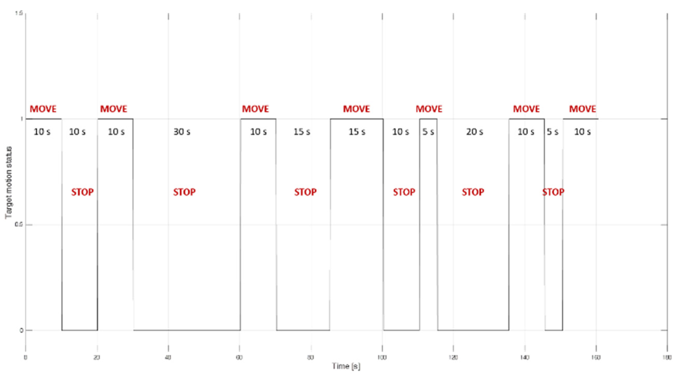
The target starts from point A, namely the point of the coordinates (−15 m, 40 m) of the grid. It moves with an angle α = 45° with respect to the x-axis, with a constant velocity along both axes ( v x = v y = 1 m s v = 1.4 m s ). It stops two times before reaching point B (15 m, 40 m). After a few seconds where the target is stationary there, it moves again towards point C, and finally, it comes back to starting point A. The time duration of each interval for the considered trajectory is reported in Figure 6. In this figure, the value of 1 represents the intervals where the target is moving with a uniform linear motion, whereas the value of 0 indicates the intervals where the target is stationary. It is clear that the six intervals labeled with the word “STOP” correspond to the six yellow crosses in Figure 5.
The measurements defined with this procedure represent the ground truth, which is the real path of the target. In order to simulate the measurements provided by the sensors, we injected a Gaussian additive noise into the available ground truth. Specifically, for the purposes of these simulated analyses, both sensors were assumed to share the same measurement accuracies, and this was kept constant along the target path. Their positioning errors were generated as zero-mean Gaussian random variables with the same standard deviations for both the x and y components:
σ x ( P B R ) ( k ) = σ x ( P S L ) ( k ) = σ x = 2   m , σ y ( P B R ) ( k ) = σ y ( P S L ) ( k ) = σ y = 2   m
We observe that this is an unrealistic assumption, since the measurement error variances for both sensors are functions of the target position via the local SNR and the local projection of the native measurements errors resulting from the solution of the 2D localization problem at each sensor. However, we deliberately assume this hypothesis in order to focus on the benefits of the proposed fusion strategy when both sensors potentially convey the same amount of information on the current target position. The values in (27) will also be used in the filtering stage and, specifically, in (10). With reference to the available measurements, we assumed that the sensors provided the position estimates each T = 0.5 s.
According to the characteristics of the employed sensors, described in detail in Section 2, the simulated PSL sensor is assumed to provide a position estimated each T seconds, regardless of the target motion status. In contrast, the PBR provides its estimates only when the target is moving; therefore, we generated radar measurements only for the “MOVE” intervals.
The main parameters of the employed filters, namely the standard deviations of the model errors and the Markov transition matrix P , are reported in Table 3. For the KF, the standard deviations of the model errors are set with higher values in order to reduce the errors when the target changes its motion status.
The rest of this section is devoted to a detailed analysis of the accuracy of the proposed multi-sensor processing scheme, in comparison to the standard approaches. We explicitly noticed that our strategy is based on specific hypotheses about the presence or absence of PBR measurements depending on the target motion; however, for passive radar, it is necessary to consider even nonideal cases that could be found in real applications.
Therefore, in the following sections, we consider both ideal and nonideal conditions. The ideal conditions refer to the case when all the measurements from both sensors are present (with the PBR measurements only missing for the stationary targets), and all of them are relevant to the considered target (i.e., no false measurements are included in the set). This case represents a benchmark for the proposed fusion strategy and is considered in Section 4.2, where we study the behavior of the position Root Mean Square Error (RMSE) for our multi-sensor fusion technique with respect to the standard filters.
Although this hypothesis is very useful to study the conceptual operation of the proposed technique, it is unrealistic when studying the applications in a real scenario. Therefore, it is removed in Section 4.3, where different values are tested for the probability of having a correct target detection (hence, an available measurement) and the probability of having false plots. The RMSE analysis is then repeated in order to prove the effectiveness of the proposed multi-sensor fusion approach under typical conditions and to investigate its robustness in more challenging situations.

4.2. Evaluation of the RMSE under Ideal Conditions

The analysis of the RMSE during the entire simulation time allows us to observe the behaviors of the five approaches mentioned in the initial part of this section with respect to the motion status of the target. To achieve this purpose, N = 1000 trials of Monte Carlo simulations were run.
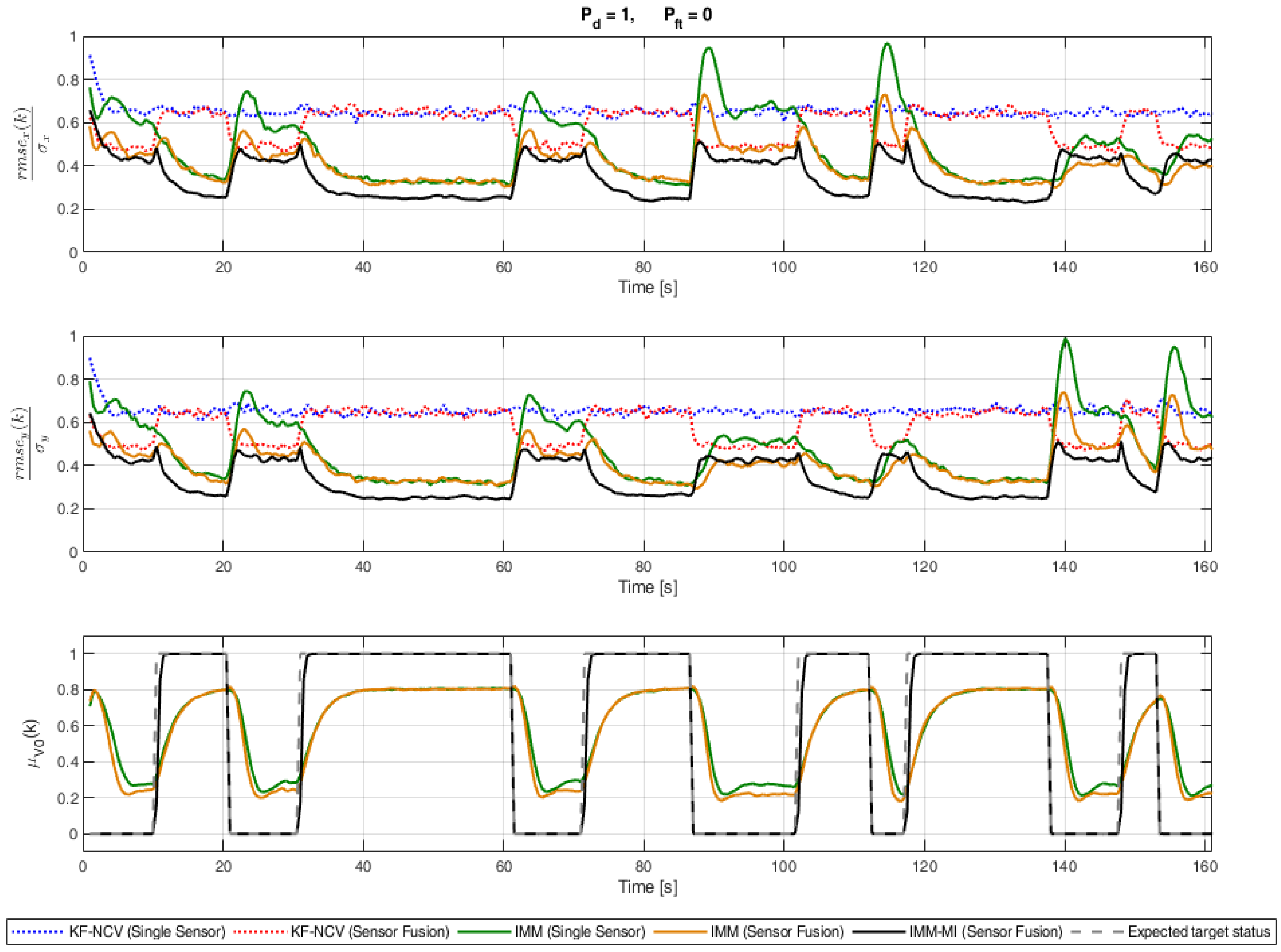
The results performed under ideal conditions are reported in Figure 7, whose first two subplots show the normalized RMSE with respect to the x-axis and the y-axis, respectively, whereas the third one presents the V0 model probabilities of the filters within the IMM structure, compared with the expected target status ( μ V 0 ( k ) = 1 for STOP, and μ V 0 ( k ) = 0 for MOVE) that is drawn with a grey, dashed line. As apparent, the model probability of the KF is not reported, since it is composed of just one model; therefore, μ V 0 ( K F ) ( k ) will be always 0.
The main outcomes of the performed analysis can be summarized by three main points:
(1)
On average, the sensor fusion version of a specific tracking strategy provides an enhanced performance with respect to the single sensor version of the same strategy.
(2)
On average, the IMM filters provide better performances than the KF when the same number of sensors is used.
(3)
The IMM-MI filter (black solid line) outperforms the other strategies for almost the entire simulation.
In particular, a very good performance can be achieved when the target is stationary and the IMM-MI allows a reduction of the error of about 75% with respect to the use of the raw measurements, for which the normalized RMSE is equal to 1. This is due to the capability of the proposed strategy to impose the correct target velocity selection ( v = 0   m / s ). In the same intervals, the error reduction (with respect to the use of the raw measurements) is limited to 60–65% for the classical IMM filter, due to the conflict between the NCV and V0 models, and to only about 30–35% for the KF-NCV (the higher error of the KF-NCV is partially due to the differences between the values of σ a x shown in Table 3, which is necessary to reduce the error of the KF-NCV in the transient states, since the KF is not devised to manage fast changes of the dynamics, as better illustrated in the following section).
The difference between the IMM-MI filter and other strategies is less evident in MOVE intervals, since the filter has to estimate by itself the correct target velocity when the target starts to move again. However, even when the target changes its motion status, the IMM-MI filter is still the best approach.
Proper considerations have to be made for the portions of trajectory where the target moves orthogonally to the axes. In fact, we can observe what happens after the third (about 85 s) and the fourth (about 110 s) stops, when the target starts again to move orthogonally to the y-axis. In these cases, the classical IMM filter results in a drastic increase of the error along the x-component (first subplot in Figure 7). This can be explained by considering that, in this portion of the path, the target is stationary with respect to the y-axis while moving along the x-axis, but the model probability is the same for the two directions. In these conditions, the choice between the two motion models is more difficult for the classical IMM filter, and its capability of recognizing the target motion is reduced. This confirms that the classical IMM filter is not appropriate to face the problem of move-stop-move target tracking. In contrast, for the same reason, the IMM-MI filter does not provide the lowest error for the RMSE calculated over the y-axis (second subplot in Figure 7) in the same transition intervals, since it increases the probability of choosing the NCV model, which is not the real target behavior along the y-axis. Nevertheless, the increase of the error for the IMM-MI filter is negligible, since the achieved values are not too high, and they occur for a very short time. Analogous considerations can be made for the last segment of the path, this time for the y component.
In addition, by observing the V0 model probability reported in Figure 7, it is evident that the new approach increases the capability that the tracking filter follows the correct target behavior. The numerical comparison of the analyzed approaches is reported in Table 4, where the normalized RMSE is shown for the entire simulation and the transient and the steady states, separately.
It is evident that the exploitation of two complementary sensors (PBR and PSL) and the information about the presence of PBR measurements for the innovation modification is a good solution for this problem, as this strategy helps to choose the correct model when it operates in the ideal conditions.

4.3. Evaluation of the RMSE under Non-Ideal Conditions for the PBR Sensor

Unlike in the ideal case, the PBR sensor operating against a real scenario is subject to a certain fraction of missed detections, which can be caused by the presence of thermal noise, as well as by multipath fading or interferences. Moreover, in some cases, measurements are provided even when the target is stationary, again as a result of the thermal noise or interferences.
Since our strategy is strongly based on the presence or absence of PBR measurements, we emulate the nonideal situation by defining the PBR detection and false alarm probabilities as follows:
  • Missing PBR measurements when the target is moving are emulated through the definition of the Detection Probability, P d , which is used for the generation of the radar measurements during the “MOVE” intervals.
  • The presence of “False Plots” when the target is stationary that are erroneously associated with the target are emulated by defining the False Target Probability, P f t .
While the test in Section 4.2 was performed under ideal conditions, P d = 1 ,     P f t = 0 , we carried out the same tests under nonideal conditions, characterized by P d = 0.9 ,     P f t = 10 2 . The resulting plot, obtained under these conditions, hardly shows any differences from the ideal case shown in Figure 7. Similarly, the results of a performance analysis obtained as a function of the Pd, only showed differences in the second decimal digit from the results in Table 4. This clearly shows that the proposed scheme is robust to the presence of a nonideal PBR performance.
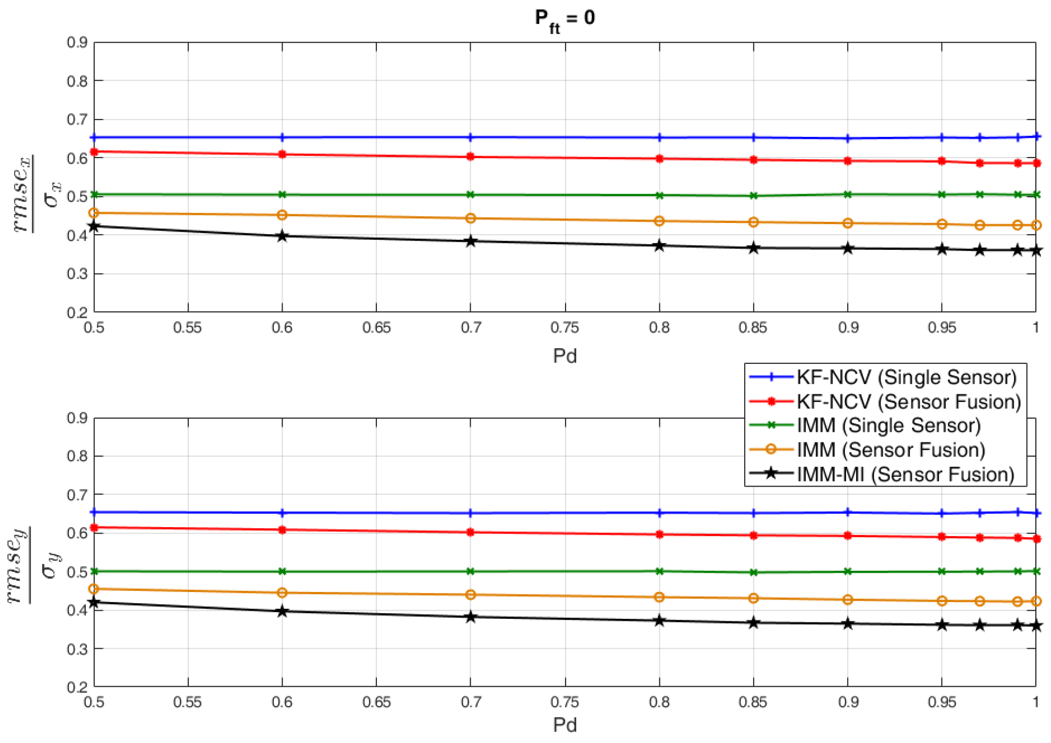
To further analyze the performance of our technique when a higher number of PBR missed detections are present, in Figure 8, we set P f t = 0 and plotted the normalized RMSE, averaged over the entire simulation, as a function of P d .
It is interesting to notice that the IMM-MI filter (black line) provides the best performance in terms of the positioning accuracies for all the values of P d . This improvement is larger for the highest values of P d , namely when the MOVE condition is always characterized by the presence of measurement, but even for P d = 0.5 , there is some improvement with respect to the standard IMM fusion filter.
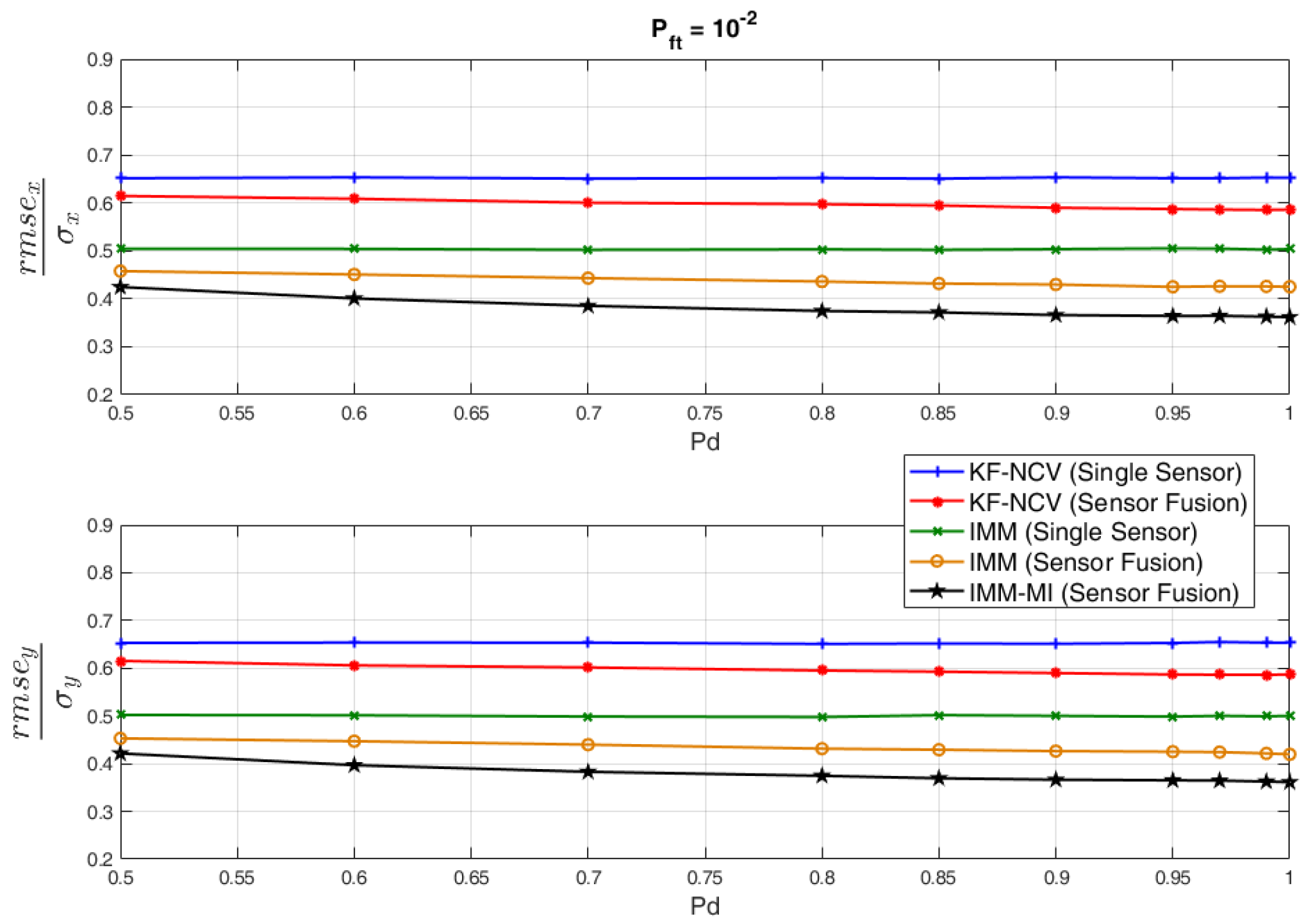
Figure 9 reports the results of a similar analysis, performed for the same scenario and the same sensor parameters but with P f t = 10 2 . In this way, the IMM-MI filter is further stressed, with the purpose of quantifying its limitations when the operating conditions are unfavorable. As apparent, the performance of the filter is not sensibly affected, even by the presence of such a reasonably high false alarm rate. Therefore, the considerations above also apply to this case, which confirms the robustness of the proposed approach. This is not an obvious result, since the proposed fusion strategy relies on the assumption of missing PBR measurements for the stationary targets, and its robustness to a reasonably high false alarm rate suggests that this is suitable for real scenarios.

5. Tests on the Experimental Data

Aiming at validating the IMM-MI filter for real-world applications, we compared the previous strategies against the experimental data. Specifically, two examples of move-stop-move targets are presented hereafter.
The first test case is represented by a human target carrying an active mobile device, namely a smartphone, surfing the web through a Wi-Fi signal (Section 5.2). The second example is dedicated to a drone, which streams its webcam video and flight data to the Radio Controller through their Wi-Fi connection (Section 5.3).
The specific characteristics of these two experiments are reported in Table 5, whereas the experimental equipment used for both experiments is described in Section 5.1 below.

5.1. Experimental Equipment and Operational Conditions

The experimental measurements were collected in an outdoor environment (a parking area in Cisterna di Latina). The system setup, sketched in Figure 1, was implemented using USRP 2955 by National Instruments as the four-channel Rx and four commercial receiving antennas (TP-LINK TL-ANT2409A). These antennas are characterized by a horizontal beam width of about 60° and a peak gain of 9dBi. Moreover, a commercial wireless AP (D-Link DAP 1160) was used as the illuminator of the opportunity for the passive radar system. This is configured to transmit on channel 5 of the Wi-Fi band (2.432 GHz), with a Beacon Interval (BI) set to 3 milliseconds, which defines the Pulse Repetition Time (PRT) of the passive radar.
We used a different Wi-Fi channel for the PSL, which requires sampling the down-converted signal with a high sampling rate (40 MHz in our specific case) and to separate the two channels by the appropriate filtering of the collected data. Thereafter, the Wi-Fi packets are extracted and decoded from each one of the two filtered signals. This allows us to classify the acquired packets based on the transmitting source and, therefore, to associate them either with the AP or the target (device/drone).
After the association of the packets, for both the PBR and PSL a coherent integration is performed separately over all the packets received from each source in constant time intervals of 0.5 s. This provided both an increased value of SNR (compared to the single packet) and a set of synchronous measurements (thus circumventing the additional difficulties caused by the asynchronous nature of the Wi-Fi packet reception). Specifically, the AoA, bistatic range and TDoA measurements were extracted after the coherent integration stage at the same temporal instants with a rate of 2 Hz.
The proposed sensor fusion technique was applied to these measurements and compared to the standard processing techniques. Unlike for the simulated case, where both sensors were assumed to share the same accuracies for the x and y measurements, the appropriate standard deviations were used in this case. These were evaluated for each target location, taking into account both the specific accuracy of the native measurements of AoA, bistatic range and TDoA (depending both on SNR and position with respect to the sensors) and the effect of the nonlinear transformation used to obtain the x and y measurements. Specifically, due to the high nonlinearity of the short-range positioning problem, and taking into consideration the acquisition geometry used in the reported tests (see Figure 10 and Figure 15), proper approximations were considered to quantify the accuracy degradation when moving from a near-range reference location to a far-range position.
For the single-node PBR sensor exploiting a single bistatic range estimate and a single AoA estimate, the standard deviations of the measurement errors are approximated as:
σ x ( P B R ) ( k ) σ x N ( P B R ) · [ y ( k ) y N ] 3 σ y ( P B R ) ( k ) σ y N ( P B R ) · [ y ( k ) y N ] 2
where the dependence is mostly on the current y(k) coordinate of the target position. The values of the standard deviations at y N   (near range) are set based on the results in reference [9], taking into account the estimated SNR.
For the dual-node PSL sensor exploiting two AoA estimates, the measurement accuracy degradation along the y-axis is approximated as
σ x ( P S L ) ( k ) σ x N ( P S L ) · [ y ( k ) y N ] 2 σ y ( P S L ) ( k ) σ y N ( P S L ) · { 1 + [ y ( k ) x B ] 2 1 + ( y N x B ) 2 } 3 2
where x B is the x coordinate of the Node B location.

5.2. Experimental Results against Human Targets

For this experiment, the four USRP receiving channels were connected to four surveillance antennas, arranged to provide the dual-node system in Figure 3 operating with strategy #2 for the PSL (see Section 2.3), namely two AoAs were used, and the PBR transmitted signal must be reconstructed from the surveillance channels. Two receiving antennas were located near the receiver with 14 cm of space between them. The other two antennas were placed 25 m apart, with the same spacing among them.
A Cartesian reference system and a square grid identical to Figure 5 was replicated on the ground, and its points were used for the calibration of the AoA measurements. The position of the two nodes, as well as the nominal target path, are sketched out in Figure 10. The AP was placed at the midpoint of the baseline between the two nodes, namely point (11.4 m, 5.25 m).
The nominal motion of the target with the active mobile device in this coordinate system can be described as:
  • motion from point A (−15 m, 40 m) to point B (15 m, 70 m) in 19 s,
  • stop in point B for 8 s,
  • motion from point B to point C (15 m, 40 m) in 14 s,
  • stop in point C for 10 s and
  • motion from point C to point A in 14 s.
To evaluate the potentialities of the proposed sensor fusion technique against a realistic scenario, we assumed that the mobile device carried by the human target also performs some upload activity. To this purpose, a smartphone in Hotspot mode was used, co-located with the AP, to allow for the mobile device to upload a video on a server. This was set on channel 1 of the Wi-Fi band (2.412 GHz). During the whole acquisition time, the user was active in the upload. However, a person typically uses a mobile device more when not moving; therefore, the transmission of the video occurred mainly during the stop intervals.
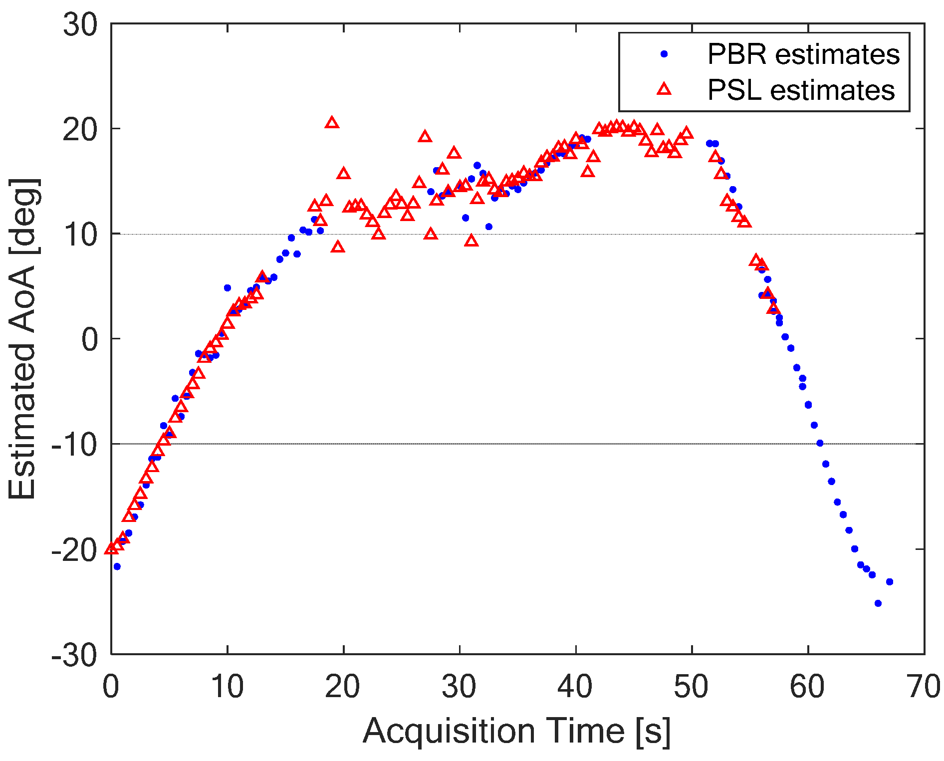
The complementarity of the PBR and PSL is evident in Figure 11, where the AoA measurements for the two sensors are compared. In fact, the AoA estimates of the PSL sensor (red triangles) compensate for the lack of measurements of the PBR sensor (blue dots) when the target is stationary (from 18 s to 27 s and from 40 s to 50 s). On the other hand, the PBR guarantees a continuity of the high-rate measurements when the target is moving and the person interrupts the transmission of the video or the communication is over (producing a scarcity of PSL measurements).
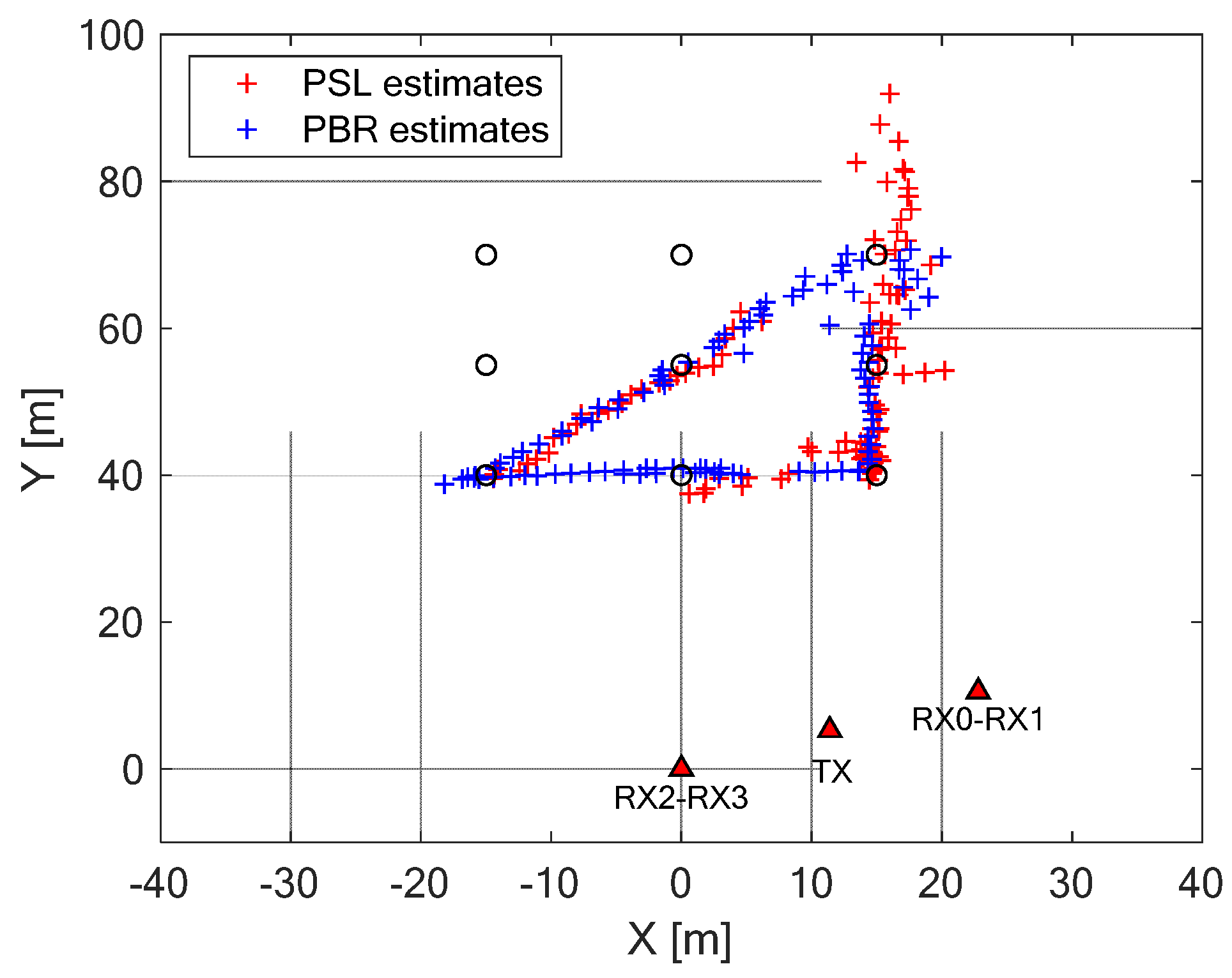
Figure 12 shows the conversion of the individual PSL (red crosses) and PBR (blue crosses) measurements on the x-y plane. In this figure, it is evident that both the PSL and PBR are effective for short-range human target localizations. However, each one of the sensors presents gaps in the measurement continuity in some portions of the path. Moreover, there are points (for example, for y > 60 m) where the position estimates are less accurate, especially for the PSL, providing estimates that vary around the actual position. The error in these estimates could be probably increased by the proximity of a building (as can be seen in Figure 10) and, in particular, of a metallic fence present on the right side of the reference square grid and by the greater distance between the target and receiver. This consideration matches with the results shown in references [6,9].
In general, these results are consistent with the idea that passive radar provides more accurate position estimates with respect to the device-based technique, whereas the PSL has a key role when the target is stationary and the PBR does not provide measurements.
The proposed data fusion technique was applied to this set of measurements and compared to the same standard processing techniques considered for the simulated analysis of Section 4 using the same parameter values reported in Table 3.
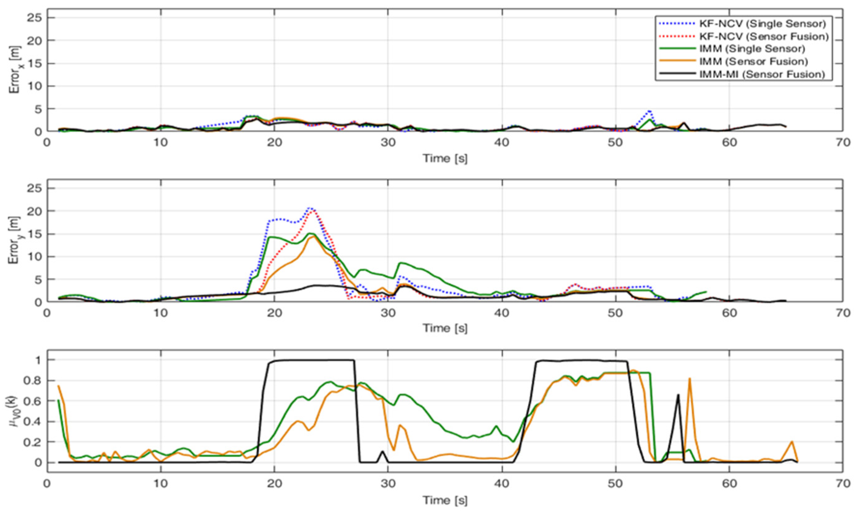
The results for the instantaneous positioning errors of the five approaches are reported in Figure 13. As expected, the highest errors occur during the stops when the target is stationary and only the PSL provides information about the target location. In particular, during the first stop, the quality of the PSL measurements is affected by the distance from the receiving antennas and the proximity to the metallic fence and the building.
We notice that the IMM filters provide generally better accuracy than the KF filters in the stop conditions, especially when fusing the two sensors. However, the proposed IMM-MI sensor fusion scheme is the strategy that mostly contains the errors even in the presence of the inaccurate PSL measurements. On average, it outperforms the other strategies, allowing us to continuously measure the positions of both moving and stationary targets without gaps of continuity. Moreover, the lower subplot in Figure 13 clearly shows its capability in identifying the correct motion model. In fact, the model probabilities (black line) reach values very close to 1 or 0 in the correct time frames. Clearly, a worse accuracy and probability of identification of the correct motion status are provided by the other IMM schemes.
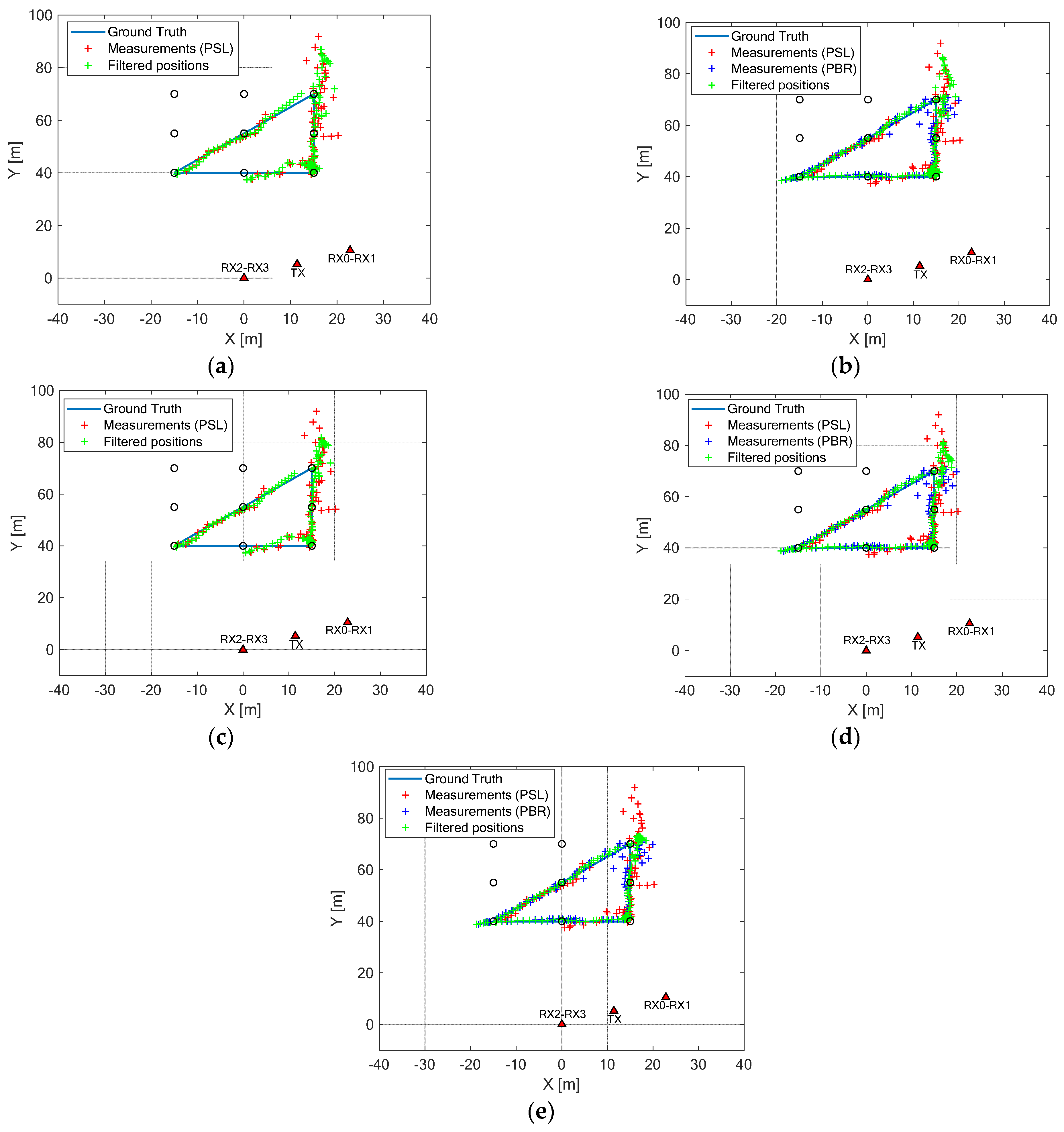
This behavior is also evident from Figure 14 showing the localization on the x-y -plane obtained with the different methodologies above. Figure 14a shows that the selected value, namely σ a x = σ a y = 2   m / s 2 for the KF-NCV model error, provides a small difference between the raw PSL measurements (red crosses) and the filtered positions (green crosses).
Figure 14b for the sensor fusion KF-NCV filter shows that the exploitation of the PBR measurements (blue crosses) helps the tracker follow the actual target motion, thanks to the possibility to (i) rely on more accurate position estimates and (ii) compensate for the lack of measurements of the PSL sensor when the target is moving but it is not involved in the upload activities. On the other hand, the PSL is necessary to know the target position when the target is stationary.
Similar considerations apply to the IMM filter (Single Sensor) shown in Figure 14c and the IMM (Sensor Fusion), presented in Figure 14d. However, the IMM filter allows to better limit the error compared to the KF-NCV when the target changes its motion status during the first stop.
Finally, the results of the IMM-MI sensor fusion scheme are reported in Figure 14e. The proposed strategy provides a further performance improvement, which is apparent:
  • in the motion interval, where smoothed filtered positions are provided, which are very close to the line of the ground truth, and
  • in the two stop intervals, where the variations around the points (15 m, 40 m) and (15 m, 70 m) are smaller with respect to those shown for the standard methodologies.
A numerical assessment of the accuracy improvement provided by this methodology is shown in Table 6. The reduction in the total error is apparent when the IMM-MI sensor fusion scheme is applied (see the last row of Table 6). In particular, the errors are comparable with those achieved by the PBR, but the percentage of the acquisition covered by the IMM-MI approaches 100% thanks to the fusion of the two sensors measurements, whereas the PBR only does not exceed a coverage of 74% with the selected target path.
The previous considerations confirmed that, even in the real application, the proposed technique, which combines Data Fusion and an appropriate modification of the IMM, represents an effective solution for target localization and tracking in short-range applications.
We noticed that the preliminary results for the human targets were presented in reference [5]; however, the acquisition was performed with the condition of low data traffic for the PSL sensor: only the connection activities between the AP and device were considered, since the AP was not allowed to upload the data. Moreover, a directional antenna with a higher gain was used for the AP. The PBR provided accurate position estimates, while the PSL was effective but provided a small number of measurements. In contrast with the results shown in reference [5], this time, the PSL provided a number of measurement estimates comparable to the PBR. This provided generally better performances for both the PSL single sensor and for the data fusion techniques included in our proposed approach.

5.3. Experimental Results against Commercial Drones

For this experiment, the three USRP receiving channels were connected to three surveillance antennas, and the fourth channel was connected to the AP (providing the reference signal for the PBR sensor), arranged to provide the dual-node system in Figure 3 operating with strategy #1 for the PSL (see Section 2.3); namely, an AoA and a TDoA were used.
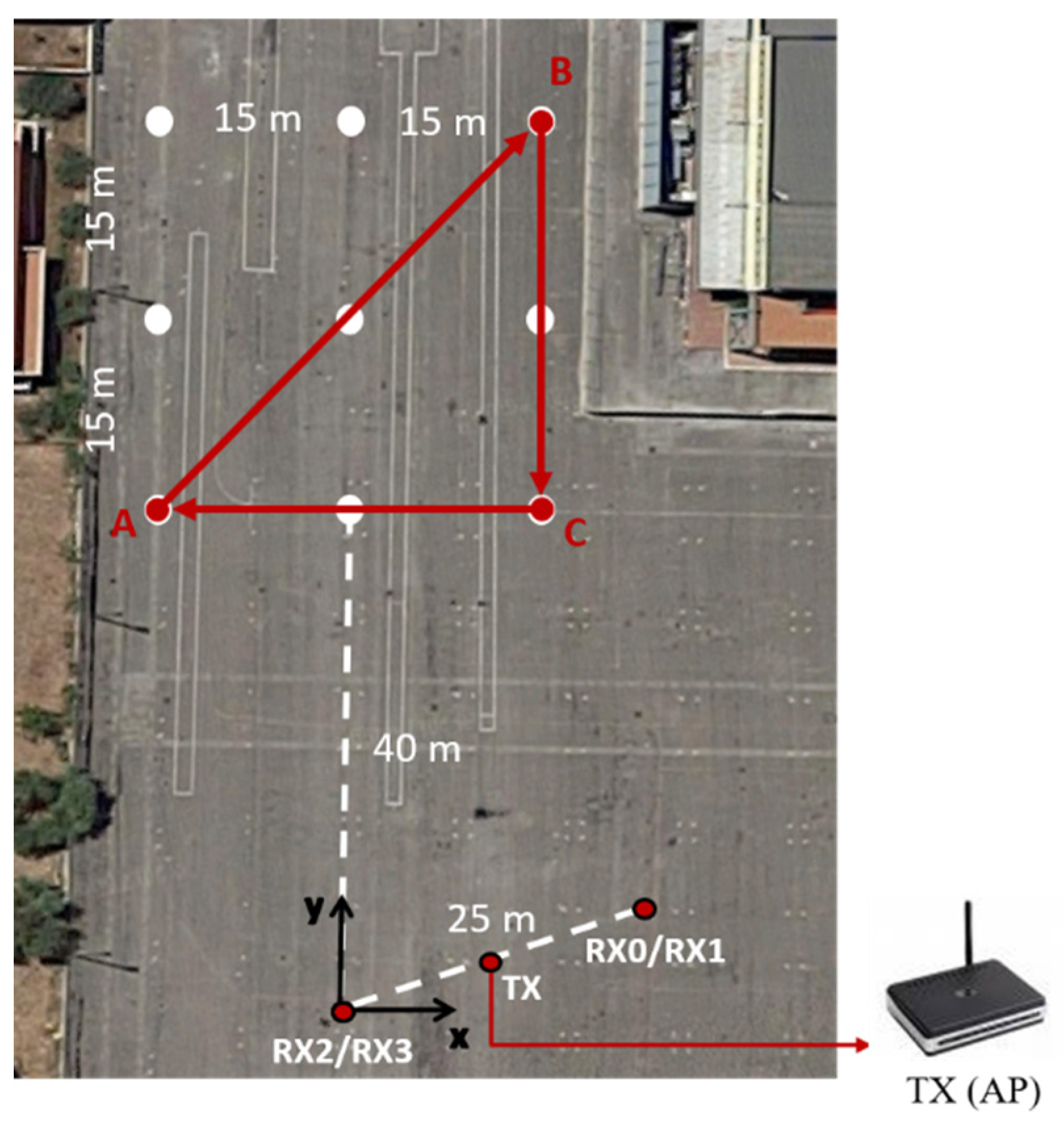
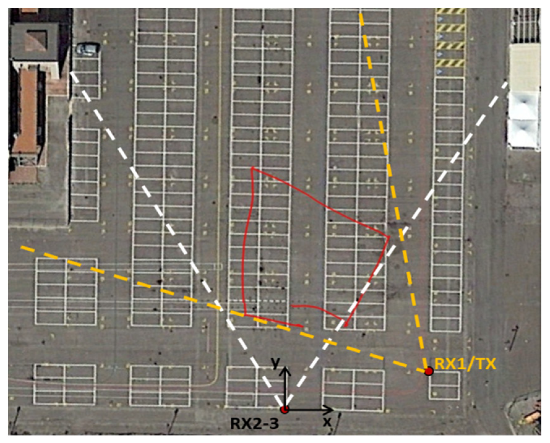
Two receiving antennas were located near the receiver with 14 cm of space between them. The third antenna and the AP were placed 25 m apart. Figure 15 shows the test area, together with a sketch of the position of both nodes and their nominal beam-widths.
To evaluate the effectiveness of the proposed scheme against the drone targets, we used a widely available DJI Mavic Pro commercial drone. It is a lightweight (about 730 g) drone with small size (about 30 × 25 × 8 cm), Wi-Fi 802.11a/b/g/n/ac connectivity, integrated GPS/GLONASS positioning system and integrated camera for photos and videos. Its path (the ground truth) is shown in Figure 15 by the red quadrilateral polygon that was obtained from the drone’s GPS data. In this test, the drone started to fly to the point closest to the first node (RX2-3 in the figure) and turned clockwise until the end of its path. It stopped its motion in each vertex of the quadrilateral polygon. The height of the drone ranged from 1.2 to 1.5 m; the antennas of both nodes were installed at about 1.5 m above the ground. This setup allowed us to avoid the additional errors expected for a 2D positioning of noncoplanar targets.
In this case, the Wi-Fi communications from drone to controller (Real-Time Video or Flight Data Information exchange) could be used for the drone position estimation through the PSL technique. The streaming video transmission of the drone was set on Wi-Fi channel 9 (2.452 GHz). Moreover, the same AP used for human targets was exploited as the source of opportunity for the PBR sensor.
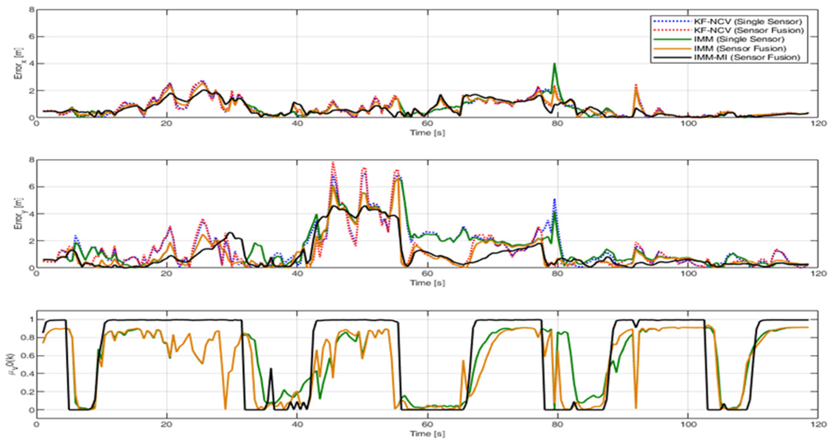
The results for the positioning errors of the considered filters are reported in the first two subplots of Figure 16 for the x and y components, respectively, whereas the identification of the stop and motion conditions is provided by the third subplot. As apparent, the highest errors are present during the stop times, when the PBR measurements are not available and the drone is possibly affected by the yaw, pitch and roll motion components that make the PSL measurements less stable and accurate than they were during the motion intervals. Again, the single sensor operation does not provide the best results, whereas the sensor fusion provides better results—in particular, when exploiting the IMM approach. Despite the higher residual errors, the five methodologies have a similar behavior presented when applied to human targets, as can be seen when comparing Figure 13 and Figure 16.
Again, the IMM-MI approach provides the best performance for almost the entire acquisition duration in terms of positioning accuracy and capability of target motion recognition. The information about the stop condition of the target, provided by the absence of PBR measurements, is nicely exploited to identify the stop condition so that the best filtering is applied to the measurements.
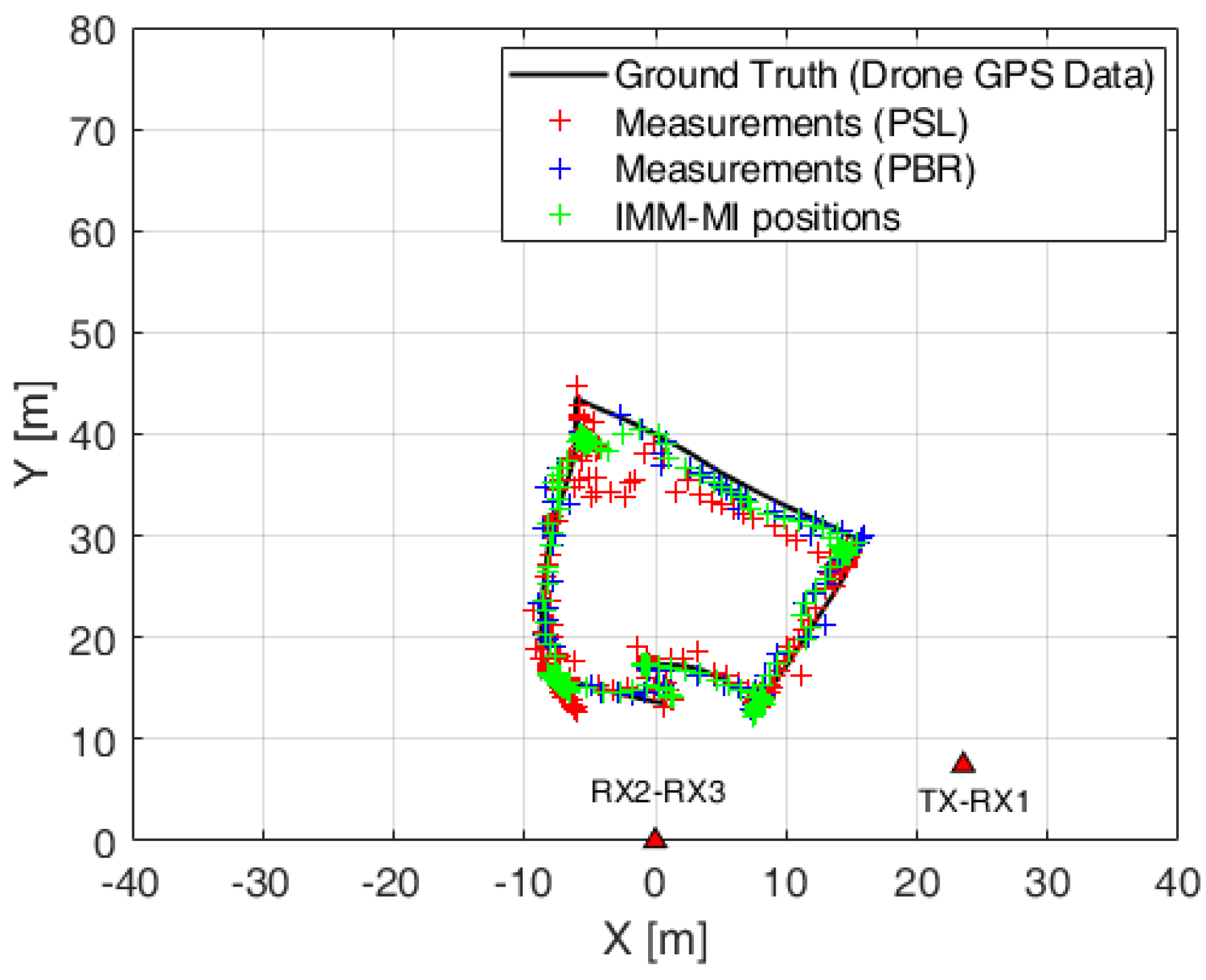
Finally, to evaluate the effectiveness of the proposed sensor fusion approach against the live scenario, in Figure 17, we report the drone positions estimated by the PSL (red crosses), PBR (blue crosses) and the position after the application of the proposed IMM-MI approach (green crosses). These results are compared with the ground truth, which, in this case, is represented by the drone GPS data (black solid line). This plot on the x-y plane makes it more evident that the IMM-MI is a valid solution for the drone’s surveillance, combining the good quality of PBR estimates with the gapless PSL position measurements achievable by exploiting the direct drone emissions. In fact, due to the small dimensions of the drone used for this experimental test, the PBR was able to estimate the drone location for a smaller fraction of the whole trajectory than in the human target case. The fusion of PBR and PSL sensibly improved the continuity of the measurements and effectively used the identification of the stop intervals to improve the performance.

6. Conclusions

In this work we showed that the PBR and PSL measurements are complementary, since the former provides accurate target positioning only during the target motion phases, whereas the latter provides somewhat coarser measurements but with high continuity. Their fusion is able to provide a significant benefit for targets characterized by a move-stop-move type of motion behavior, such as, for example, human beings and commercial drones.
To capitalize on the sensor fusion for such targets, in this paper, we introduced a modified version of the IMM filter scheme aimed at fusing the measurements of two complementary positioning techniques based on Wi-Fi signals: Passive Bistatic Radar (PBR) and Passive Source Location (PSL) sensors for a move-stop-move-type target, like a human target or a drone. The modified innovation (MI) evaluation introduced in the IMM fusion filter allows us to exploit the absence of the PBR measurements during the stop intervals to identify these intervals and to optimize the filtering operations under such conditions.
The performance of the proposed processing scheme was evaluated both by means of simulated data and by two experiments specifically devoted to human targets and small UAVs in local area environments. The results of the analyses showed that the fusion of the PBR and PSL measurements was able to provide significant improvements with respect to the single sensor approaches, both in the stop and in the motion intervals. Moreover, the proposed IMM-MI fusion scheme applied to the considered sensors was demonstrated to be effective for the localization and tracking of move-stop-move targets, providing the best performance in terms of the positioning accuracy, target motion recognition capability and continuity in target tracking.

Author Contributions

Conceptualization, I.M., C.B., F.C. and P.L.; methodology, I.M., C.B., F.C. and P.L.; software, I.M., C.B., F.C. and P.L.; validation, I.M., C.B., F.C. and P.L.; formal analysis, I.M., C.B., F.C. and P.L.; investigation, I.M., C.B., F.C. and P.L.; data curation, I.M., C.B., F.C. and P.L.; writing—original draft preparation, I.M., C.B., F.C. and P.L. and writing—review and editing, I.M., C.B., F.C. and P.L. All authors have read and agreed to the published version of the manuscript.

Funding

This research was partially funded by Sapienza University of Rome, project Passive Radar systems for Autonomous Driving applications (PaRAD).

Institutional Review Board Statement

Not applicable.

Informed Consent Statement

Not applicable.

Data Availability Statement

Data sharing not applicable.

Conflicts of Interest

The authors declare no conflict of interest.

References

  1. De Cubber, G. Explosive Drones: How to Deal with this New Threat? In Proceedings of the 9th International Workshop on Measurement, Prevention, Protection and Management of CBRN Risks, International CBRNE Institute, Les Bons Villers, Belgium, 1 April 2019; pp. 1–8. [Google Scholar]
  2. Ritchie, M.; Fioranelli, F.; Borrion, H. Micro UAV crime prevention: Can we help Princess Leia? In Crime Prevention in the 21st Century; Savona, B.L., Ed.; Springer: New York, NY, USA, 2017; pp. 359–376. [Google Scholar]
  3. Shi, X.; Yang, C.; Xie, W.; Liang, C.; Shi, Z.; Chen, J. Anti-Drone System with Multiple Surveillance Technologies: Architecture, Implementation, and Challenges. IEEE Commun. Mag. 2018, 56, 68–74. [Google Scholar] [CrossRef]
  4. Lykou, G.; Moustakas, D.; Gritzalis, D. Defending Airports from UAS: A Survey on Cyber-Attacks and Counter-Drone Sensing Technologies. Sensors 2020, 20, 3537. [Google Scholar] [CrossRef] [PubMed]
  5. Milani, I.; Colone, F.; Bongioanni, C.; Lombardo, P. WiFi emission-based vs passive radar localization of human targets. IEEE 2018, 1311–1316. [Google Scholar] [CrossRef]
  6. Milani, I.; Bongioanni, C.; Colone, F.; Lombardo, P. Fusing active and passive measurements for drone localization. IEEE 2020. [Google Scholar] [CrossRef]
  7. Wireless LAN Medium Access Control (MAC) and Physical Layer (PHY) Specifications; IEEE: Piscataway Township, NJ, USA, 2016.
  8. Colone, F.; Falcone, P.; Bongioanni, C.; Lombardo, P. WiFi-Based Passive Bistatic Radar: Data Processing Schemes and Experimental Results. IEEE Trans. Aerosp. Electron. Syst. 2012, 48, 1061–1079. [Google Scholar] [CrossRef]
  9. Falcone, P.; Colone, F.; Macera, A.; Lombardo, P. Two-dimensional location of moving targets within local areas using WiFi-based multistatic passive radar. IET Radar Sonar Navig. 2014, 8, 123–131. [Google Scholar] [CrossRef]
  10. Tan, B.; Woodbridge, K.; Chetty, K. A real-time high resolution passive WiFi Doppler-radar and its applications. In Proceedings of the 2014 International Radar Conference, Lille, France, 13–17 October 2014. [Google Scholar]
  11. Rzewuski, S.; Kulpa, K.; Samczyński, P. Duty factor impact on WIFIRAD radar image quality. IEEE 2015, 400–405. [Google Scholar] [CrossRef]
  12. Li, W.; Piechocki, R.J.; Woodbridge, K.; Tang, C.; Chetty, K. Passive WiFi Radar for Human Sensing Using a Stand-Alone Access Point. IEEE Trans. Geosci. Remote. Sens. 2020, 59, 1986–1998. [Google Scholar] [CrossRef]
  13. Mazor, E.; Averbuch, A.Z.; Barshalom, Y.; Dayan, J. Interacting multiple model methods in target tracking: A survey. IEEE Trans. Aerosp. Electron. Syst. 1998, 34, 103–123. [Google Scholar] [CrossRef]
  14. Kirubarajan, T.; Bar-Shalom, Y. Tracking evasive move-stop-move targets with a GMTI radar using a VS-IMM estimator. IEEE Trans. Aerosp. Electron. Syst. 2003, 39, 1098–1103. [Google Scholar] [CrossRef]
  15. Coraluppi, S.; Carthel, C. Multiple-Hypothesis IMM (MH-IMM) Filter for Moving and Stationary Targets. In Proceedings of the 2001 International Conference on Information Fusion, Montreal, QC, Canada, 10 August 2001. [Google Scholar]
  16. Li, X.-R.; Bar-Shalom, Y. Multiple-model estimation with variable structure. IEEE Trans. Autom. Control. 1996, 41, 478–493. [Google Scholar] [CrossRef]
  17. Colone, F.; Palmarini, C.; Martelli, T.; Tilli, E. Sliding extensive cancellation algorithm for disturbance removal in passive radar. IEEE Trans. Aerosp. Electron. Syst. 2016, 52, 1309–1326. [Google Scholar] [CrossRef]
  18. Bar-Shalom, Y.; Li, X.R. Multitarget-Multisensor Tracking: Principles and Techniques; YBS Publishing: Storrs, CT, USA, 1995. [Google Scholar]
  19. Genovese, A.F. The Interacting Multiple Model Algorithm for Accurate State Estimation of Maneuvering Targets; Johns Hopkins APL Technical Digest: Laurel, MD, USA, 2001; Volume 22, pp. 614–623. [Google Scholar]
  20. Granstrom, K.; Willett, P.; Bar-Shalom, Y. Systematic approach to IMM mixing for unequal dimension states. IEEE Trans. Aerosp. Electron. Syst. 2015, 51, 2975–2986. [Google Scholar] [CrossRef]
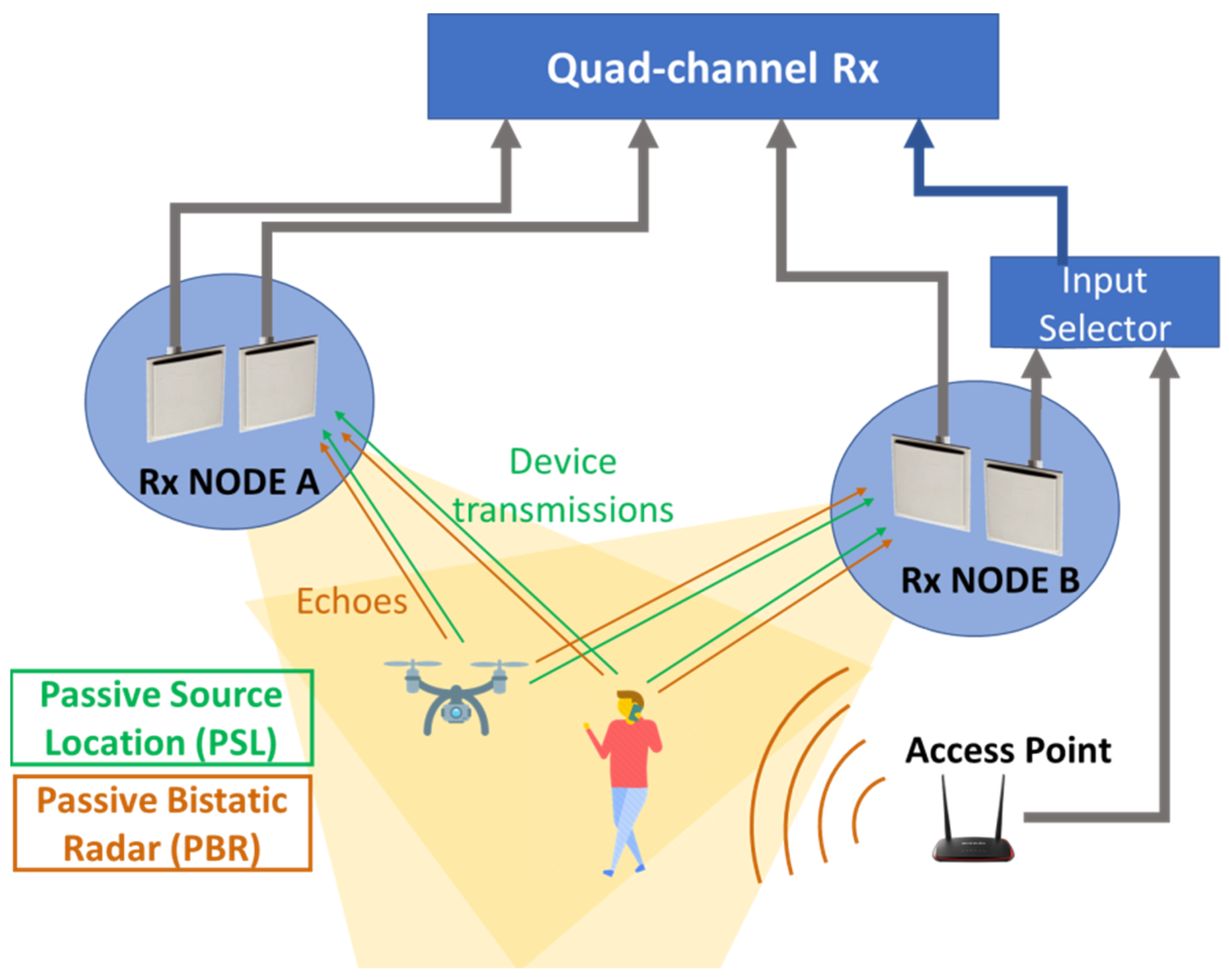
Figure 1. Sketch of a system setup implementing the PBR and PSL approaches.
Remotesensing 13 03556 g001
Figure 2. Processing scheme of the PBR exploiting a single node with two surveillance antennas.
Remotesensing 13 03556 g002
Figure 3. Processing scheme of the PSL exploiting a dual-node system.
Remotesensing 13 03556 g003
Figure 4. IMM-MI processing scheme.
Remotesensing 13 03556 g004
Figure 5. Simulated trajectory.
Remotesensing 13 03556 g005
Figure 6. Target motion description: value = 1, the target is moving; value = 0, the target is stationary.
Remotesensing 13 03556 g006
Figure 7. Comparison of the normalized positioning RMSE with respect to the x-axis (top) and the y-axis (center) over a simulated move-stop-move target for P d = 1 and P ft = 0 . In the subplot at the bottom is the relative V0 model probability.
Remotesensing 13 03556 g007
Figure 8. Comparison of the normalized positioning RMSE averaged over the entire simulation vs. P d , with respect to the x-axis (top) and the y-axis (bottom), over a simulated move-stop-move target for P ft = 0 .
Remotesensing 13 03556 g008
Figure 9. Comparison of the normalized positioning averaged over the entire simulation vs. P d , with respect to the x-axis (top) and the y-axis (bottom) over a simulated move-stop-move target for P ft = 10 2 .
Remotesensing 13 03556 g009
Figure 10. Experimental setup and nominal path for the human target case.
Remotesensing 13 03556 g010
Figure 11. Comparison between the AoA estimations with the PBR technique and PSL technique.
Remotesensing 13 03556 g011
Figure 12. Comparison of the PSL and the PBR localizations on the x-y plane.
Remotesensing 13 03556 g012
Figure 13. Positioning errors and V0 model probabilities in the experimental data for human target localization and tracking.
Remotesensing 13 03556 g013
Figure 14. The localization and tracking of human targets on the x-y plane with: (a) the KF-NCV (Single Sensor), (b) KF-NCV (Sensor Fusion), (c) IMM (Single Sensor), (d) IMM (Sensor Fusion) and (e) IMM-MI (Sensor Fusion).
Remotesensing 13 03556 g014
Figure 15. Experimental setup and nominal path for the drone test case.
Remotesensing 13 03556 g015
Figure 16. The positioning errors and V0 model probabilities of the experimental data for the drone localization and tracking.
Remotesensing 13 03556 g016
Figure 17. Localization and tracking of the drone on the x-y plane with IMM-MI (Sensor Fusion).
Remotesensing 13 03556 g017
Table 1. The PBR and PSL features.
Passive Bistatic Radar
(PBR)
Passive Source Location
(PSL)
Higher computational costLower computational cost
Closely spaced targets
cannot be discriminated
Closely spaced targets can be discriminated based on their MAC address
No detection of stationary targetsStationary targets can be detected
and localized
Effective for moving targetsPotentially inaccurate for moving targets
Device-free localizationDevice-based localization
Table 2. Summary of the operations performed at each block of an IMM scheme.
Filtering
NCV model-based filter
State prediction s ^ 1 ( k | k 1 ) = Φ 1 ( k 1 ) s ^ 01 ( k 1 | k 1 )
Prediction covariance P 1 ( k | k 1 ) =
      Φ 1 ( k 1 ) P 01 ( k 1 | k 1 ) Φ 1 T ( k 1 ) + Q 1 ( k 1 )
Innovation r 1 ( k ) = z ( k ) H N s ( k ) s ^ 1 ( k | k 1 )
Innovation Covariance S 1 ( k ) = H N s ( k ) P 1 ( k | k 1 ) H N s T ( k ) + R ( k )
Kalman Gain K 1 ( k ) = P 1 ( k | k 1 ) H N s T ( k ) S 1 1 ( k )
Filtered state s ^ 1 ( k | k ) = s ^ 1 ( k | k 1 ) + K 1 ( k ) r 1 ( k )
Filtered state covariance P 1 ( k | k ) = P 1 ( k | k 1 ) K 1 ( k ) S 1 ( k ) K 1 T ( k )
V0 model-based filter
State prediction s ^ 2 ( R ) ( k | k 1 ) = Φ 2 ( k 1 ) s ^ 02 ( R ) ( k 1 | k 1 )
Prediction covariance P 2 ( R ) ( k | k 1 ) =
Φ 2 ( k 1 ) P 02 ( R ) ( k 1 | k 1 ) Φ 2 T ( k 1 ) + Q 2 ( k 1 )
Innovation r 2 ( k ) = z ( k ) ( 1 N s ( k ) × 1 I 2 × 2 ) s ^ 2 ( R ) ( k | k 1 )
Innovation Covariance S 2 ( k ) = ( 1 N s ( k ) × 1 I 2 × 2 ) P 2 ( R ) ( k | k 1 ) ( 1 N s ( k ) × 1 I 2 × 2 ) T + R ( k )
Kalman Gain K 2 ( k ) = P 2 ( R ) ( k | k 1 ) ( 1 N s ( k ) × 1 I 2 × 2 ) T S 2 1 ( k )
Filtered state s ^ 2 ( R ) ( k | k ) = s ^ 2 ( R ) ( k | k 1 ) + K 2 ( k ) r 2 ( k )
Filtered state covariance P 2 ( R ) ( k | k ) = P 2 ( R ) ( k | k 1 ) K 2 ( k ) S 2 ( k ) K 2 T ( k )
Augmentation/Reduction
AugmentationUniform distribution augmentation [20]:
s ^ 2 ( R ) ( k | k ) s ^ 2 ( k | k )
P 2 ( R ) ( k | k ) P 2 ( k | k )
ReductionRemove the velocity components from the augmented structures:
s ^ 02 ( k | k ) s ^ 02 ( R ) ( k | k )
P 02 ( k | k ) P 02 ( R ) ( k | k )
Interaction          ( i , j = 1 , 2 )
State interaction s ^ 0 j ( k 1 | k 1 ) = μ 1 | j ( k 1 | k 1 )   s ^ 1 ( k 1 | k 1 ) + μ 2 | j ( k 1 | k 1 )   s ^ 2 ( k 1 | k 1 )
Delta state δ i | j = s ^ i ( k 1 | k 1 ) s ^ 0 j ( k 1 | k 1 ) ]
Interaction state Covariance P 0 j ( k 1 | k 1 ) =
      μ 1 | j ( k 1 | k 1 ) { P ^ 1 ( k 1 | k 1 ) + δ 1 | j δ 1 | j T } +
      μ 2 | j ( k 1 | k 1 ) { P ^ 2 ( k 1 | k 1 ) + δ 2 | j δ 2 | j T }
Combination
State combination s ^ ( k | k ) = μ 1 ( k ) s ^ 1 ( k | k ) + μ 2 ( k ) s ^ 2 ( k | k )
State difference ε j ( k ) = s ^ j ( k | k ) s ^ ( k | k )  ( j = 1 , 2 )
Combination Covariance P ( k | k ) = μ 1 ( k ) · { P ^ 1 ( k | k ) + ε 1 ( k ) ε 1 T ( k ) } +
μ 2 ( k ) · { P ^ 2 ( k | k ) + ε 2 ( k ) ε 2 T ( k ) }
Probability update          ( i , j = 1 , 2 )
Mixing probabilities μ i | j ( k 1 | k 1 ) = 1 c ¯ j p i j μ i ( k 1 )
Normalization factor c ¯ j = p 1 j μ 1 ( k 1 ) + p 2 j μ 2 ( k 1 )
Mode probabilities μ j ( k ) = Λ j ( k ) c ¯ j Λ 1 ( k ) c ¯ 1 + Λ 2 ( k ) c ¯ 2
Likelihood Λ j ( k ) = 1 | 2 π S j ( k ) | · e x p { 1 2 r j T ( k ) S j 1 ( k ) r j ( k ) }
Table 3. Settings of the employed methodologies.
Approach σ a x = σ a y
( m / s 2 )
σ v x = σ v y
( m s )
P
KF-NCV
(SINGLE SENSOR)
2--
KF-NCV
(SENSOR FUSION)
2--
IMM
(SINGLE SENSOR)
10.5 [ 0.95 0.05 0.05 0.95 ]
IMM
(SENSOR FUSION)
10.5 [ 0.95 0.05 0.05 0.95 ]
IMM-MI
(SENSOR FUSION)
10.5 [ 0.95 0.05 0.05 0.95 ]
Table 4. Comparison of the performances of different tracking techniques on the simulated target under ideal conditions.
Entire SimulationTransient StateSteady State
r m s e x σ x   r m s e y σ y   r m s e p o s σ p o s   r m s e x σ x   r m s e y σ y   r m s e p o s σ p o s   r m s e x σ x   r m s e y σ y   r m s e p o s σ p o s
KF-NCV
(SINGLE SENSOR)
0.660.650.650.660.650.650.650.650.65
KF-NCV
(SENSOR FUSION)
0.590.590.590.580.570.570.590.590.59
IMM
(SINGLE SENSOR)
0.500.500.500.620.620.620.470.470.47
IMM
(SENSOR FUSION)
0.430.420.420.510.500.510.410.400.41
IMM-MI
(SENSOR FUSION)
0.360.360.360.420.420.420.350.350.35
Table 5. Characteristics of the proposed test cases.
Test CaseNode Used for PBRPBR MeasurementsNodes Used for PSLPSL Measurements
Human targetNode A, with 2 antenna elements (reference signal reconstructed)AoA + Bistatic RangeNodes A & B, each one with 2 antenna elementsAoA + AoA
DroneNode A, with 2 antenna elements (reference signal obtained from the AP)AoA + Bistatic RangeNodes A with 2 antenna elements & Node B with 1 antenna elementAoA + TDoA
Table 6. Comparisons of the performances achieved by the different tracking techniques in the human target case.
ApproachMEAN ERROR X
(m)
STD ERROR X
(m)
MEAN ERROR Y
(m)
STD ERROR Y
(m)
MEAN ERROR POS
(m)
STD ERROR POS
(m)
MEASUREMENTS AVAILABILITY across the Observation Time
PSL MEASURES0.890.993.785.384.025.3779%
PBR MEASURES1.030.920.910.701.491.0174%
KF-NCV
(SINGLE SENSOR)
0.800.893.373.903.573.9179%
KF-NCV
(SENSOR FUSION)
0.860.842.163.322.503.30100%
IMM
(SINGLE SENSOR)
0.850.903.323.103.503.1479%
IMM
(SENSOR FUSION)
0.880.861.802.162.142.20100%
IMM-MI
(SENSOR FUSION)
0.850.751.260.851.630.96100%
Publisher’s Note: MDPI stays neutral with regard to jurisdictional claims in published maps and institutional affiliations.