Abstract
Groundwater has a significant contribution to water storage and is considered to be one of the sources for agricultural irrigation; industrial; and domestic water use. The Gravity Recovery and Climate Experiment (GRACE) satellite provides a unique opportunity to evaluate terrestrial water storage (TWS) and groundwater storage (GWS) at a large spatial scale. However; the coarse resolution of GRACE limits its ability to investigate the water storage change at a small scale. It is; therefore; needed to improve the resolution of GRACE data at a spatial scale applicable for regional-level studies. In this study; a machine-learning-based downscaling random forest model (RFM) and artificial neural network (ANN) model were developed to downscale GRACE data (TWS and GWS) from 1° to a higher resolution (0.25°). The spatial maps of downscaled TWS and GWS were generated over the Indus basin irrigation system (IBIS). Variations in TWS of GRACE in combination with geospatial variables; including digital elevation model (DEM), slope; aspect; and hydrological variables; including soil moisture; evapotranspiration; rainfall; surface runoff; canopy water; and temperature; were used. The geospatial and hydrological variables could potentially contribute to; or correlate with; GRACE TWS. The RFM outperformed the ANN model and results show Pearson correlation coefficient (R) (0.97), root mean square error (RMSE) (11.83 mm), mean absolute error (MAE) (7.71 mm), and Nash–Sutcliffe efficiency (NSE) (0.94) while comparing with the training dataset from 2003 to 2016. These results indicate the suitability of RFM to downscale GRACE data at a regional scale. The downscaled GWS data were analyzed; and we observed that the region has lost GWS of about −9.54 ± 1.27 km3 at the rate of −0.68 ± 0.09 km3/year from 2003 to 2016. The validation results showed that R between downscaled GWS and observational wells GWS are 0.67 and 0.77 at seasonal and annual scales with a confidence level of 95%, respectively. It can; therefore; be concluded that the RFM has the potential to downscale GRACE data at a spatial scale suitable to predict GWS at regional scales.
1. Introduction
Groundwater has become the main source of irrigation and domestic water supplies. It is being abstracted at an alarming rate due to its easy access and wider distribution. Recently, groundwater abstraction and consumption have been increased due to an increase in population and, consequently, stress on agriculture. The level of groundwater is continuously declining due to over-abstraction as well as deteriorating water quality. The situation demands continuous groundwater monitoring and management at a regional scale [1,2,3,4]. Traditionally, a network of observational wells is used to monitor groundwater behavior at a regional scale. However, establishing such networks is not only costly but also tiresome to collect data. The spatial distribution of such a network is uneven, which hinders the capture of variability in groundwater [5]. Therefore, the study of changes in groundwater storage at a large scale is normally constrained because observational wells data have less density and limitation of the spatial extent [6].
To this end, the deficiency is fulfilled with the usage of data from an earth gravity satellite, i.e., GRACE. It provides the opportunity for direct measurement of spatial changes in water storage with high precision and monthly resolutions [7,8,9,10,11] at a large-scale basin with reasonable accuracy [12,13,14]. Using the GRACE data, GWS can be obtained continuously at regular intervals as compared to monitoring groundwater with a network of piezometers, which is helpful to overcome the problems of scarcity and uneven distribution of piezometers in the study area. Scanlon et al. [13] observed regional water storage changes using GRACE data with an error of less than 1 cm for an area of more than 400,000 km2. Richey et al. [14] estimated global groundwater storage variation and found severe abstractions in various regions over the world, including the IBIS from 2003 to 2013. Tang et al. [15] applied the Budyko model to reconstruct annual GWS using GRACE and other multiple input variables and observed the depletion of GWS in Punjab province, Pakistan, from 1980 to 2015. Iqbal et al. [16] reported significant groundwater storage loss in this province from 2003 to 2010 using GRACE data. Although GRACE is being used widely for measuring GWS changes, its lower spatial resolution is a constraint for using this product at a small scale [13,17,18,19]. Therefore, it is essential to downscale GRACE data at a reasonable resolution that could be useful for estimating GWS changes at regional scales.
Two main approaches of spatial downscaling available are dynamic downscaling and statistical downscaling [17,20,21]. Dynamic downscaling is used to develop a numerical model at a higher resolution, which can be applied at smaller scales in local areas. While statistical downscaling approaches are applied using observations taken over several years to develop the relationship between data from large-scale and data from small-scale observations. Different from the dynamic downscaling approach, which requires complex data from multiple sources, the statistical downscaling approach is flexible to develop modeling factors at a higher resolution. For example, multivariate statistical regression uses fewer auxiliary data and is less time-consuming; hence, it significantly improves the spatial resolution of hydrological variables. A statistical-based downscaling of TWS using a water balance equation to improve the spatial resolution of TWS was proposed by Ning et al. [22]. They observed that evapotranspiration, surface runoff, rainfall, and other hydrological variables have a comprehensive effect on TWS. Yin et al. [23] downscaled GWS using high-resolution evapotranspiration (ET) data and concluded that the spatial resolution of GWS can be improved effectively for the case study of the North China plain.
The machine-learning techniques are excellent, and they can be applied effectively to downscale hydrological variables [24,25,26]. For example, Seyoum et al. [27] estimated the glacial aquifer GWS based on downscaling using a machine-learning approach and observed that the resolution of GWS could be improved at a spatial scale despite the limitations in input data uncertainties. Miro et al. [19] used an artificial neural network model to conduct downscaling for the central basin of California and found that the downscaling model could accurately simulate the variations in GWS at high resolution. Rahaman et al. [28] used the random forest algorithm to downscale GRACE-derived GWS of 1° at a high resolution (0.25°) for the Northern High Plains aquifer, and the NSE reached 0.58~0.84. Sun. [29] utilized GRACE data and the artificial neural network model to predict the variations in GWS in the United States. The authors concluded that the model outputs showed some limitations in spatial prediction but changes in the time series of GWS could be predicted well. Yang et al. [30] reconstructed TWS using linear regression and a machine-learning approach using GRACE and GLDAS products in Northwest China from 1948 to 2002. The results show that canopy water, soil moisture, and snow water equivalent are closely related to TWS.
Keeping in view the limitations identified by the researchers, this study proposed a two-step machine-learning-based downscaling model. At first, TWS downscaling was conducted and, then, isolating other vertical water components of TWS to acquire downscaled GWS output. The TWS is a complex hydrological variable that has other vertical water storage components, e.g., soil moisture, canopy water, surface runoff, snow water equivalent, and groundwater [31,32].
Since the random forest model is data-driven, the quality and nature of the data used as inputs are of critical importance. However, a previous study by Chen et al. [33] that employed a random forest model to predict TWS and GWS utilized hydrologic variables that are combinations of evapotranspiration, rainfall, soil moisture, surface runoff, canopy water, and snow water equivalent and just investigated the model accuracy. Here, we extend this work. The main contribution and novelty of this study are:
- We used temperature from a previous study by Zhang et al. [34] and other key local geospatial datasets (elevation, slope, and aspect) to increase the accuracy of the model along with GRACE data that are shown in the literature to be significant predictors of TWS [34,35].
- We assessed the trend and estimated the loss of downscaled GWS based on RFM.
- We explored the correlation of input variables with the GRACE TWS data.
In this case study, nine modeling variables were selected, including rainfall (RF), evapotranspiration (ET), soil moisture (SM), surface runoff (Qs), canopy water (CW), temperature, slope, aspect, and digital elevation model (DEM) and analyzed using a random forest machine-learning model to downscale GRACE-derived TWS spatially in space-time. However, a random forest model has been used to downscale GRACE data by very few researchers.
To date, however, there are no downscaled products that exist for IBIS, although these products are very important for local water resources management. Considering the lack of high-precision and high-resolution GWS products, our research concentrated mainly to construct a higher-accuracy model and, for the first time, produces a continuous yearly change in TWS (including GWS) over the IBIS using the machine-learning method. The objectives of this study are threefold:
- Integrate the GRACE TWS data with other hydrological and geospatial variables into the RFM to downscale GRACE-derived TWS and GWS from 1° to 0.25° for the IBIS.
- Validate the downscaled GWS with observational wells GWS.
- Assess the trend variability and slope of downscaled GWS by utilizing the Mann–Kendall trend test and Theil–Sen’s estimator.
2. Materials and Methods
2.1. Study Area
The area selected for this study is the Pakistani part of the Indus basin irrigation system (IBIS) (Figure 1). The IBIS encompasses approximately 201,072 km2 area. The river flows comprise glacier melt, snowmelt, rainfall, and runoff. Outside the polar regions, the upper Indus River basin contains the greatest area of perennial glacial ice in the world (220,00 km2). The glaciers serve as natural storage reservoirs that provide perennial supplies to the Indus River and some of its tributaries [36]. The Indus River system forms a link between two large natural reservoirs, the snow and glaciers in the mountains and the groundwater contained by the alluvium in the Indus plains of the Sindh and Punjab provinces of Pakistan [37].
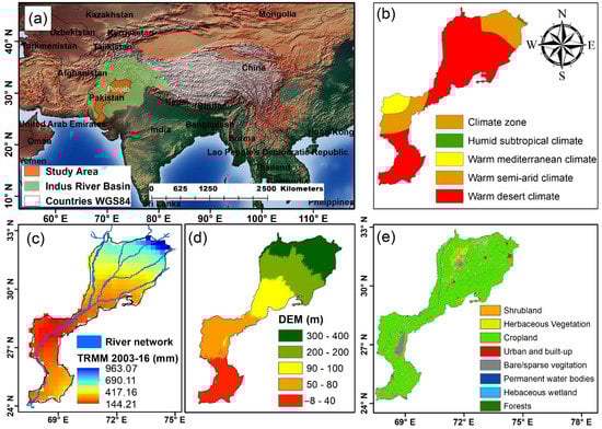
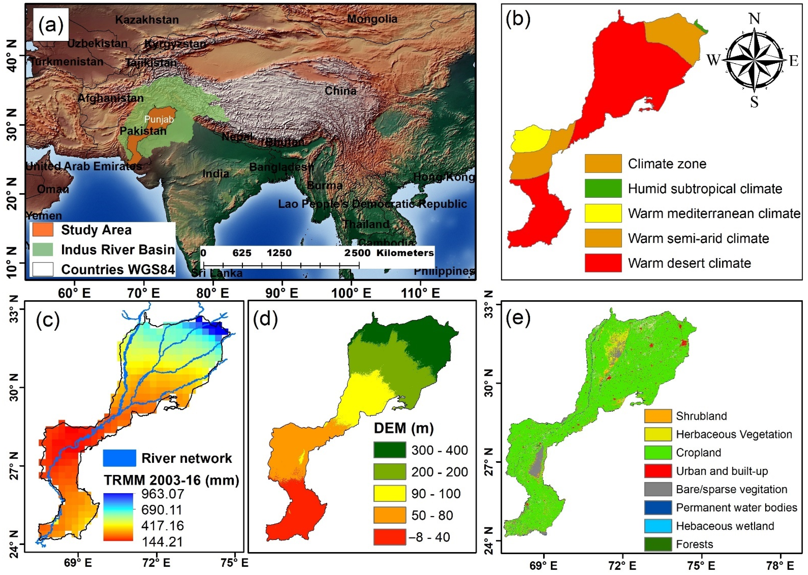
Figure 1.
(a) The Indus River basin and the study area IBIS. The background layer contains the countries and shaded relief layers from the Natural Earth dataset (http://www.naturalearthdata.com/downloads/) accessed on 21 April 2021, (b) the climatic zones according to Koppen Geiger Climate Classification, (c) average rainfall from TRMM, (d) digital elevation model (90 m) derived from Shuttle Radar Topographic Mission (SRTM), (e) land use and land cover change for 2016 (https://lcviewer.vito.be/2016) accessed on 10 May 2021.
With the rapid increase in agricultural development, population growth, and industry, water resources scarcity has become one of the significant aspects in the study area. Recently, the region has over-abstracted groundwater to meet the requirements of residential uses and agricultural production [16]. Thus, studying GWS has practical significance in the IBIS. The arid to semi-arid climate exists in the major part of the IBIS and the secondary source of water is rainfall. The seasonal rainfall from November to April during the dry Rabi season is only 30% of the total water available. May to October is the rainy Kharif season [38] providing 70% of available water.
Crop intensity and crop water requirement have increased over the past decades at the system scale in the IBIS, and have not been satisfied by the combination of surface water withdrawals and rainfall [39]. Unreliability and inadequacy of surface water supply have forced farmers to abstract groundwater resources. The quantity of groundwater resources pumping varying from 52 to 61 km3/y was reported [40,41]. The declining groundwater level is experienced in most of the north-eastern regions of Punjab where fresh groundwater is abundant [42]. Mainly, groundwater depletion in eastern Punjab is a hotspot, where the transient effect of pumping extensive groundwater across the Indo Pak borders increases the likelihood of water table depletion [43,44]. The quality of groundwater is marginal to brackish in 60% of the IBIS aquifer [45,46,47].
2.2. Data Sources and Processing
There are three databases used in this study: (i) TWS data from the GRACE satellite; (ii) soil moisture, surface runoff, canopy water, temperature, and evapotranspiration data from the global land surface assimilation system (GLDAS) NOAH model; (iii) rainfall data from TRMM 3B43. The downloaded gridded GRACE data have a spatial resolution of 1°, and the other datasets have a spatial resolution of 0.25°. The data were observed from January 2003 to December 2016, with monthly temporal resolution. Table 1 summarizes the data used in this study.

Table 1.
Summary of the data used.
2.3. GRACE TWS
The gridded GRACE satellite data (RL-05, level-3) are processed and provided by three institutions Center for Space Research (CSR, the University of Texas), Jet Propulsion Laboratory (JPL, Pasadena, CA, USA), and GeoForschungsZentrum Potsdam (GFZ, Potsdam, Germany), respectively [48,49]. It can be downloaded from here (https://grace.jpl.nasa.gov/data/get-data/monthly-mass-grids-land/) which was accessed on 13 September 2019. These three gridded GRACE products have a spatial resolution of 1° × 1° We used the average data of these three products. These products have undergone pre-processing, such as de-striping filter, Gaussian smoothing, and glacier isostatic adjustment (GIA) [33]. By averaging these TWS products, the accuracy can be improved [48,50]. Linear interpolation was used to fill all missing monthly data [51]. To restore the original signal that was lost during data processing, a multiplicative scaling factor was applied to the monthly mass gridded data provided by the GRACE satellite [27]. More information about scaling factors can be found in Landerer and Swenson [48].
2.4. GLDAS Data
The GLDAS simulates satellite and ground-based observations [52] using four land surface models, i.e., common land model (CLM), Mosaic, Noah, and variable infiltration capacity (VIC). Four land surface models provided by GLDAS-1 exists to simulate global soil moisture, surface runoff, canopy water, evapotranspiration, and other hydrological variables. The data are available from 3 h to monthly while spatial resolution is 1° × 1° [53]. This study used GLDAS-1 NOAH model data with a resolution of 0.25° × 0.25° from 2003 to 2016, which can be found on the website of the Goddard Earth Sciences Data and Information Services Center (GES DISC) (https://disc.gsfc.nasa.gov/datasets) which was accessed on 23 November 2019.
2.5. TRMM
The Tropical Rainfall Measuring Mission (TRMM) is a joint JAXA and NASA mission to monitor and study tropical rainfall and climate. The validation of the TRMM product has been carried out throughout the world [54,55,56,57,58]. The spatial resolution was aggregated to 1° from 0.25° to match with GRACE 1° data. The monthly TRMM 3B43 Version 7 (http://disc.sci.gsfc.nasa.gov/precipitation/) rainfall data for the period from 2003 to 2016 were used which was accessed on 05 October 2019.
2.6. Ground-Based Measurement
In Pakistan, groundwater levels are recorded 2 times a year from 3368 observation wells, by the Punjab Irrigation and Drainage Authority (PIDA). The data can be accessed from the PIDA website (https://irrigation.punjab.gov.pk/) which was accessed on 23 December 2020. PIDA collects groundwater data in terms of depth to water table (DTW) on seasonal bases (i) before monsoon (June) and (ii) after the monsoon (October). Certain raw observation well data had serious quality problems with irregular jumps, missing data, and outliers, which were eliminated during the data pre-processing. A subset of 398 observation wells, without having a single missing observation, is used for validation from June 2003 to June 2014 over the upper part of IBIS. The observation well data provide good estimates about the fluctuations in the groundwater table but they cannot be compared directly with GRACE-derived GWS [59]. As a result, DTW levels were converted into water level variations by subtracting the DTW from average depth to bedrock.
where GWLC is groundwater level changes, DTW is depth to the water table, and DTB is depth to bedrock (average DTB for selected observational wells = 400 m [16]).
The groundwater level anomalies at the seasonal scale were estimated by using the seasonal long-term mean from June 2003 to June 2014.
where is groundwater level anomalies, and is a long-term mean of groundwater level changes. The seasonal groundwater storage changes were estimated by multiplying average specific yield with groundwater anomalies [60].
where is groundwater storage anomalies, and is average specific yield. Specific yield is the quantity of water that is actually available for groundwater pumping when sediments or rocks are drained due to the lowering of the water table. The specific yield () in the upper part of the IBIS ranges from 0.01 to 0.4 and is between 0.07 and 0.25 in most areas [61]. The average value of , which is 0.14, was utilized to estimate ground-based [61]. The 398 observational wells location data covering the upper part of the study area (Figure 2) were analyzed and utilized to validate downscaled GWS from June 2003 to June 2014.
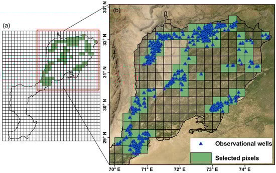
Figure 2.
(a) Watershed mask within a 0.25° × 0.25° GRACE downscaling TWS grid. (b) Observational wells located in the upper IBIS.
2.7. Data Masking for the Study Area
Figure 2a shows the IBIS watershed area overlaid with the downscaled grid cell (0.25° × 0.25°). Accordingly, the area from the intersection of the grid cell with the IBIS watershed area was calculated and was related to the amount of weight given to the IBIS watershed area to mask the gridded variables. Equations (4) and (5) were used to assign weights to estimate the variable values (e.g., TWS and GWS) for the IBIS watershed area.
where is the weight of the grid i, is the area of the IBIS watershed in grid i within the downscaled 0.25° × 0.25° grid, is the area of the grid cell i, is the spatially averaged value of one variable at a certain time (i.e., month N here) for the entire IBIS watershed, is the value of the data for grid i, A is the total area of the watershed, and n is the number of the covered grids.
3. Methodology
3.1. Groundwater Storage Estimation Using the Water Balance Equation
The water flow in and out of the system can be described by using the water balance equation (WBE). WBE estimation is difficult and complex because water balance components have uncertainties of measurements [62]. An unprecedented opportunity was provided by the GRACE satellite to capture the variability of TWS. Generally, the TWS data derived from GRACE consist of vertically integrated water storages components of the aquifer, which includes soil moisture, surface runoff, canopy water storage, and groundwater (Equation (6)) [1,3,13,28].
The WBE estimated GWS is the downscaled GWS, which is calculated using the terrestrial water balance method. An aspect of change in TWS, the other vertical water storage components that are soil moisture storage (ΔSMS), surface runoff (ΔQs), snow water equivalent (), canopy water storage (ΔCWS), and ΔGWS, observed from GLDAS, were subtracted yielding GWS [28], as shown in Equation (7).
The topography of the study region is plain with warm climate and snow is uncommon. Therefore, excluded in the estimation of ΔGWS. Here, the GLDAS data (SMS, Qs, and CWS) were also processed similarly to the GRACE anomaly. The SMS/Qs/CWS anomaly at time t was estimated using Equation (8).
where G represents SMS/Qs/CWS, and G2004–2009(avg) represents the average G from 2004 to 2009.
3.2. Mann–Kendall Trend Test
The statistic (S) of the Mann–Kendall test proposed by [63,64] is computed with the following equations given below Equation (9):
where xi and xj = values of i and j (j > i) in time series, sgn(xj − xi) is the sign function, N = number of data points, and Equation (10).
If sample size n > 10, the mean and variance are given by μ(s) = 0, Equation (11).
where ti = number of ties of extent i and m = number of tied groups.
A dataset containing similar values is called a tied group. If tie values are not present between the observations, then Equation (12).
The standard normal test statistic ZS is computed as Equation (13):
The ZS has positive and negative values, which represent the increasing and decreasing trends, respectively. The trend analysis was performed at a 5% significance level and the null hypothesis of no trend was rejected, if |ZS| > 1.96.
3.3. Artificial Neural Network (ANN)
The ANN approach develops non-linear and empirical relations between a set of “input” and response “target” variables. A series of linked units or neurons is associated with ANN that is aimed to replicate the functions of neurons in human or animal brains. They pass data between one another, a structure that enables ANNs to be trained and learn. In this study, the ANN approach utilized is called a multilayer perceptron (MLP). It consists of units known as perceptrons. It has one or more inputs, an activation function, and an output. The MLP model is developed with the combination of perceptrons in structured layers. The perceptrons are independent of each other in a given layer, but each links to the rest of the perceptrons in the following layer. Each layer consists of a set of neurons and is trained with an algorithm of back-propagation. It is one of the most extensively utilized algorithms for supervised training of multilayered neural networks [65,66,67]. It works by approximating the non-linear relation between the input and the response by varying the weight values internally. The weights with minimum error functions are then considered to be a solution to the learning problem. A comprehensive discussion on the training algorithm and neural network construction can be found in [68,69,70,71], respectively.
In this study, the ANNs are composed of one input layer, two hidden layers, and one output layer. The number of hidden neurons in our study ranged from 100 to 150. The number of epochs is the number of times the entire training data are used to update the weights. In other words, it is the number of times that the backpropagation algorithm works through the entire training dataset. This study used 100 epochs. The final model evaluation was carried out using evaluation metrics between observed and predicted values on training data.
3.4. Random Forest Model
The random forest model (RFM) is a supervised learning algorithm and was first proposed by Breiman [72] that deals with multiple classification and regression decision trees (CART) combinations. It generates homogeneous subsets of supplementary independent variables randomly at each step, which would result in a variety of trees called random forest after doing this many times [73]. RFM is not sensitive to collinearity. RFM “spreads” the variable importance across all the variables [74]. These related variables can be evaluated for similar variable importance [75]. In the aspect of modeling, it is very valuable for a nonlinear and complex problem. Generally, it is difficult to decide which variable to remove when two (or more) variables correlate with each other [76]. It utilizes the advantages of using average outcomes of each combination. Initially, it necessitates several numbers of independent variables and regression trees produced from two-thirds of the bootstrapped sample of train data individually. The remaining one-third of observations is known as out of bag (OOB).
During the classification, the number of subsets was selected taking the square root independent variables, while taking one-third of the total independent variables during regression analysis in developing the RFM. The following steps were implemented for modeling: at first, the original input data were used to train the model. The model was trained up with multiple independent variables and a response variable (dependent) using coarse resolution data. The trained RFM was tested with the independent variables to assess the model accuracy. A variable importance measure predictive (VIMP) test was performed to check the predictive power of each variable. Greater values of the VIMP test show the higher predictive power of each variable. The predicted RFM results were compared with the response variable (dependent) to compute residuals at coarse resolution. Afterward, the model was applied to the independent variables at a higher resolution (25° × 25°). Finally, the high-resolution TWS output was estimated after residual correction. The hyper-parameters of the RFM in this study were set to the defaults using the “randomForest” package of the R language [77].
The RFM is being widely utilized in remote sensing and hydrology due to its benefits in classification and regression problems [24]. The RFM has some exclusive advantages for a regression problem, which are: (1) thousands of variables can be simultaneously given to the model and it does not easy to overfitting; (2) it can run efficiently on large datasets with high accuracy; (3) the importance and interaction of variable can be detected.
We used k-fold cross validation to evaluate the robustness of the RFM. k-fold folds the dataset and takes various (random in default) portions of it to train the model, and then, tests it on the remaining instances, which is a pretty good way to check how good the model works for different train and test samples. The convention is to use 10-fold and average their results, which is more reliable.
3.5. Downscaling Model Design
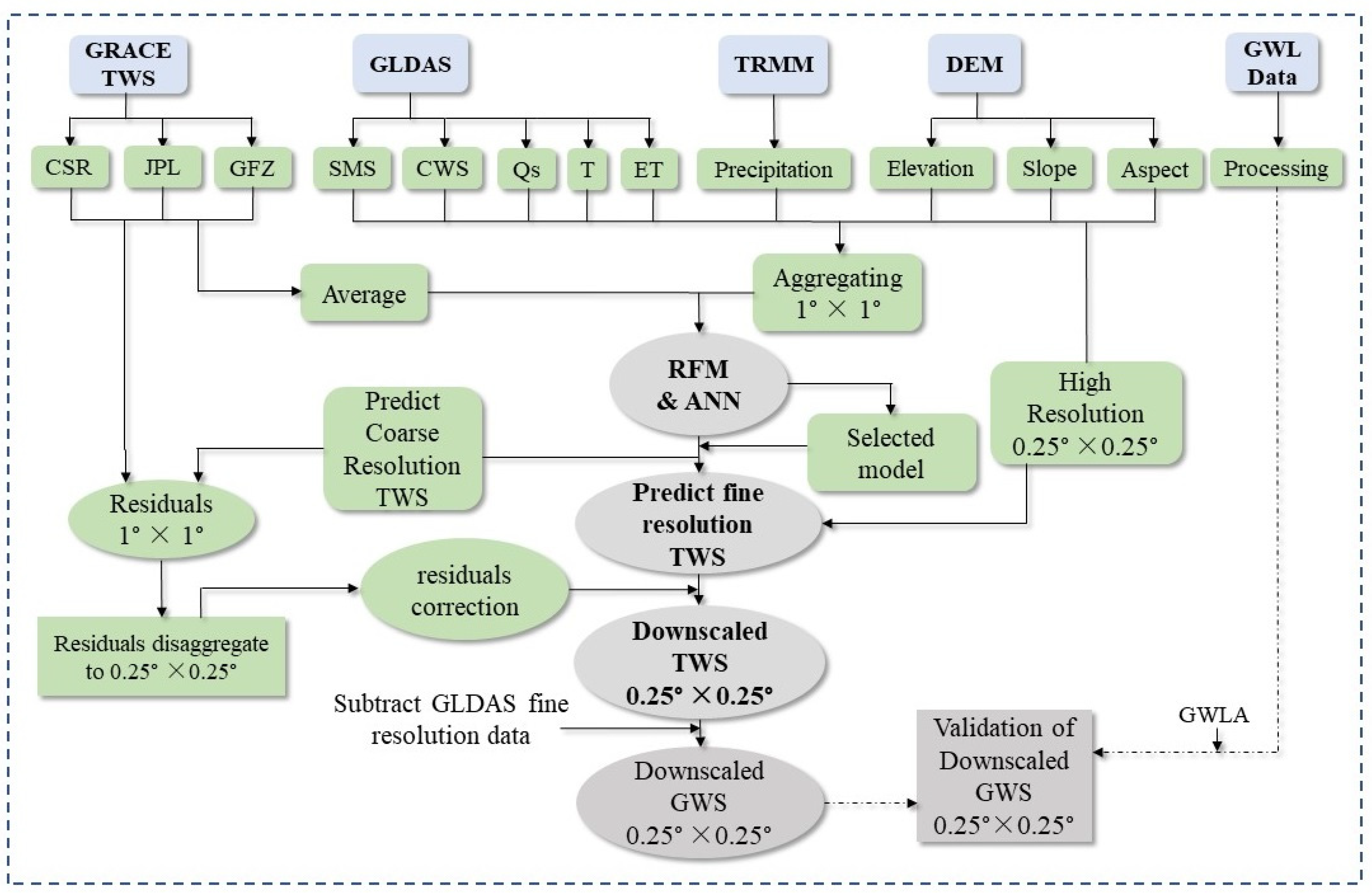
RFM and ANN model were used to downscale TWS from 1° to 0.25°. To develop both models, a statistical relationship was established between TWS, geospatial variables (elevation, slope, and aspect), and hydrological variables (soil moisture, rainfall, surface runoff, evapotranspiration, canopy water, and temperature) at coarse resolution (1°). After that, the selected model with higher correlation of coefficient was applied to the independent variables at a higher resolution (0.25°) to acquire TWS. The downscaling process of TWS from 2003 to 2016 is explained in Figure 3.

Figure 3.
Flow diagram of an integrated downscaling process in the current study.
- (1)
- At first, the nine input variables from January 2003 to December 2016 are aggregated to 1° by pixel averaging. Afterward, developed the RFM between TWS and nine hydrological and geospatial variables at a spatial resolution of 1°.
- (2)
- Secondly, the GRACE-derived TWS data deducted the predicted TWS of the RFM simulation in step (1) to calculate the residuals at a spatial resolution of 1°.
- (3)
- Thirdly, the developed RFM is applied to the hydrological and geospatial variables at a spatial resolution of 0.25° to attain the estimated 0.25° TWS of the RFM. Subsequently, the residual correction was performed at 0.25° by adding residuals to the estimated TWS at 0.25° to attain the downscaled TWS data with a spatial resolution of 0.25°. This residual correction procedure consists of three steps: the re-aggregation of the fine scale predictors (0.25°) to the original TWS resolution (1°), the calculation of TWS residuals (1°) between this new coarse scale predictors dataset (1°) and the original TWS data (1°), and the resampling (cubic convolution) of residuals (0.25°) and addition of these residuals to the fine resolution predicted TWS (0.25°), which yields the final downscaled TWS values (0.25°). The residual correction ensures that the downscaled TWS match the original data and also corrects for a prediction bias that might result from omitted variables.
- (4)
- Finally, we obtained the downscaling GWS by subtracting SMS, CWS, and Qs from the GLDAS-1 NOAH model with a spatial resolution of 0.25° from downscaling TWS. Afterward, the results were validated with the in situ water level data and the downscaled GWS.
3.6. Evaluation Methods of Model Performance
To evaluate the downscaled TWS results, four different statistical metrics were used, including R, NSE, RMSE, and MAE. Equations (14)–(17) show the mathematical representations of R, RMSE, MAE, and NSE, respectively. For R and NSE, the values closer to 1 indicate the perfect model, while for RMSE and MAE, the values close to 0 indicate the perfect model.
where Xi and Yi indicate two independent datasets with the mean value of X and Y. The input TWS is represented by Xi, and the predicted value of RFM is represented by Yi. While, N represents the total number of samples.
4. Results
4.1. Correlation Test Statistics of Model Input Variables
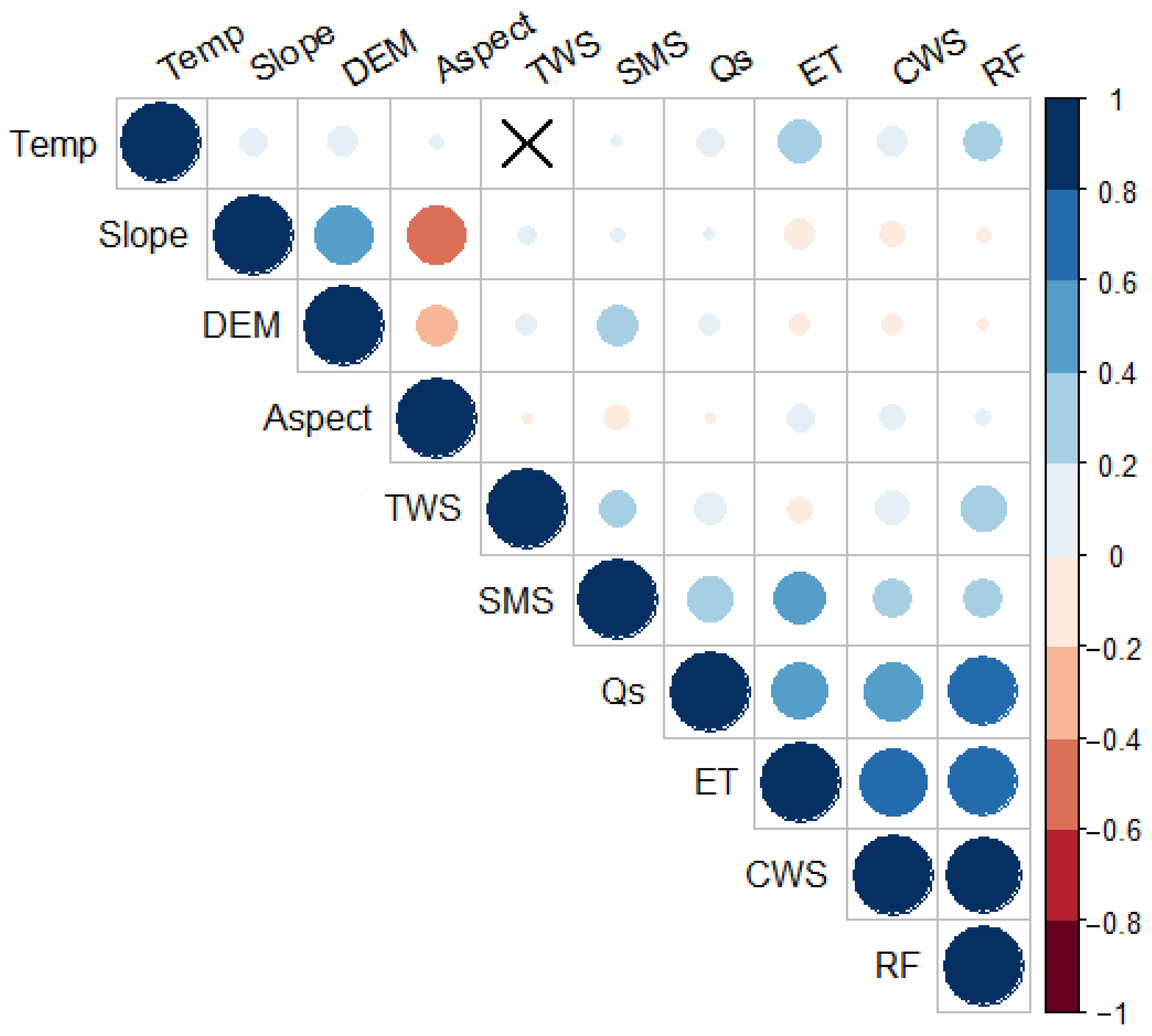
Before training RFM for downscaling, Pearson’s correlation coefficient tests were performed between all variables and were significant if p < 0.05. The relation between variables can help to determine which independent variables strongly correlate with TWS (Figure 4). This is an independent test that assists in determining the significance of variables in the trained RFM. Furthermore, it provides a secondary advantage in finding other interactions between independent variables.
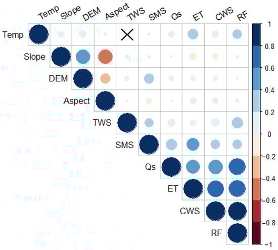
Figure 4.
Correlation plot of model input variables. The cell with an “X” indicates a statistically insignificant correlation (p < 0.05).
In decreasing order, RF, SMS, Qs, and CWS strongly correlated with GRACE TWS as shown in Figure 4. This was expected because TWS is controlled by these variables in the study region. SMS is a more spatially heterogeneous variable of how much water may be recharging the area. The weaker correlation with temperature and stronger with TWS suggests that soil moisture influence on TWS is due to replenishing in post-monsoon rather than irrigation in summer months [78]. A weak correlation between TWS and rainfall may be due to a time lag in aquifer response to rainfall [50]. The study area has high rainfall in the monsoon season. It shows a strong positive correlation with TWS. The temperature is the only independent variable that has an insignificant correlation with TWS (R = 0.01, p = 0.29). An increase in temperature will probably decrease TWS values [79]. Therefore, temperature and TWS do not show a statistical correlation. Despite this, the temperature is still included as an independent variable.
4.2. Sensitivity Analysis of RFM
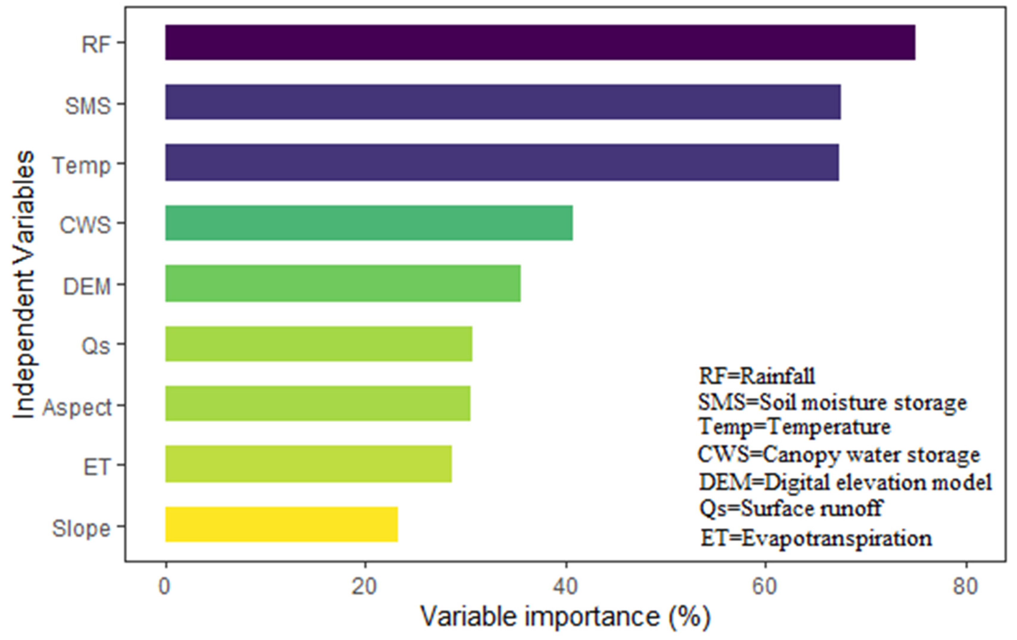
The model performance mainly depends on the selection of input variables that correlate with GRACE data strongly. The soil data, rainfall, DEM, and temperature [19,80], surface runoff [22], and evapotranspiration [23] were used to downscale the GRACE dataset. However, in this study, different independent variables, including rainfall, SMS, Qs, temperature, CWS, ET, slope, aspect, and elevation were used for developing the model (RFM). Two hypotheses were assumed, i.e., GRACE data have a non-linear relation to other independent variables, and interactions remain consistent in each spatial direction.
A variable importance measures predictive (VIMP) test was performed to check the predictability of independent variables by the model. It calculates the change for each variable in prediction error before and after permutation. VIMP values close to zero shows that the variable has less influence or is non-existent in prediction. The predictive importance of the variables for downscaling is shown in Figure 5. Figure 5 shows that rainfall (RF) was the most crucial variable in developing RFM. The slope was found to be the least important to predict TWS. Since all the variables have values above zero. Therefore, all the independent variables were considered skillful in the downscaling of TWS.
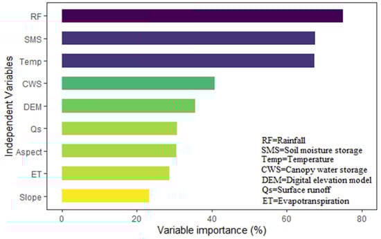
Figure 5.
Importance measures predictive (VIMP) test of the independent variables.
The VIMP of model-independent variables is consistent to some extent with the correlations to TWS observed in Figure 4. Though the order is slightly different, two variables (rainfall and SMS) strongly correlate to TWS, which are also the most influencing variables in training the RFM to predict TWS. Particularly, the temperature is also influential as soil moisture (Figure 5) in predicting TWS despite the lack of significant correlation (Figure 4). The slope has minimal influence as a predictor because of the nearly homogenous presence of surface area within the study area (Figure 1d).
4.3. Accuracy Analysis of RFM
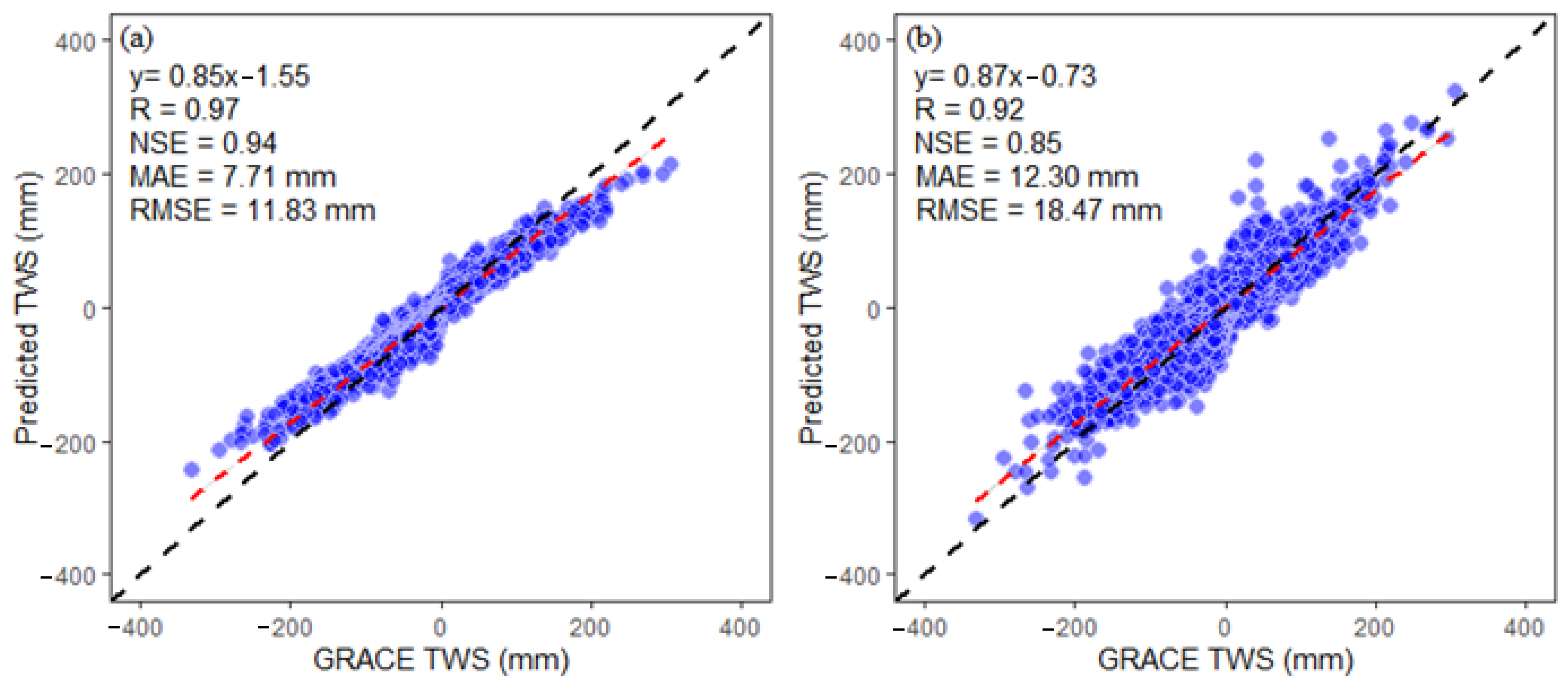
The original input data were used to train and test the model. To predict the TWS using the above-mentioned nine-input independent variables, two machine-learning models were developed. A comparison between RFM and ANN model predicted TWS and GRACE-derived TWS is provided in Figure 6. The x-axis shows the GRACE-derived TWS, and the y-axis shows the predicted TWS. In Figure 6, the RFM has R (0.97), NSE (0.94), MAE (7.71 mm), and the lowest RMSE of 11.83 mm, respectively. While, the ANN model has R (0.92), NSE (0.85), MAE (12.30 mm), and the highest RMSE of 18.47 mm. From the above results, it can be seen that downscaling RFM is the best, which can meet the requirements of variable prediction. Incorporating the geospatial variables and temperature data, the RFM shows higher accuracy than the previous studies [22,33]. It can be concluded that the RFM can accurately predict changes in TWS at a high resolution after introducing the residual correction. Therefore, this study only analyzes the output of the RFM in the following discussion.
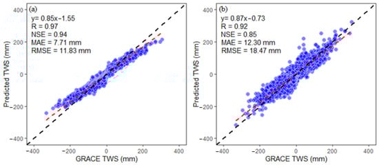
Figure 6.
Accuracy assessment of machine-learning models (a) RFM and (b) ANN with GRACE-derived TWS.
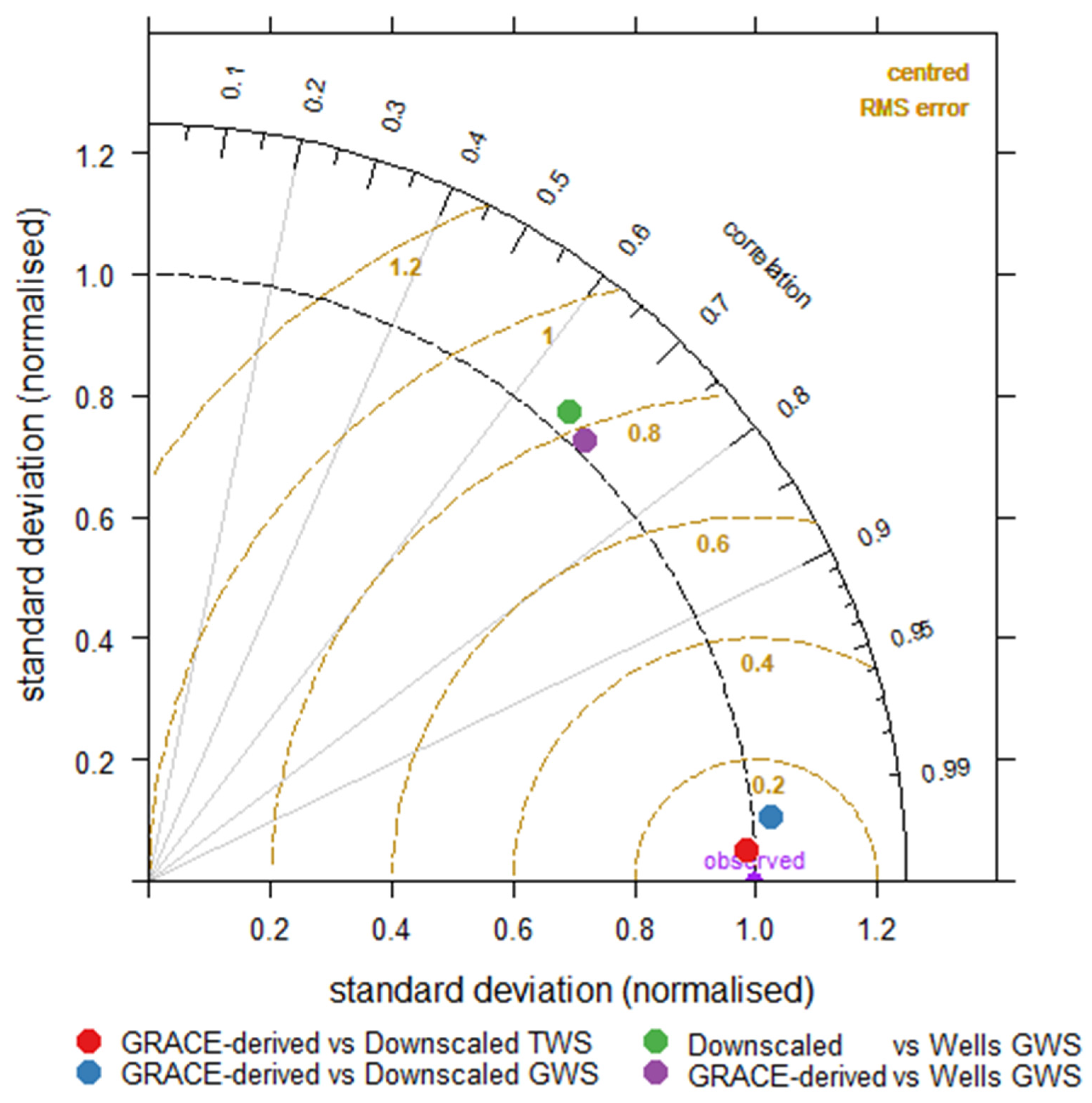
The performance of downscaled TWS and GWS against GRACE-derived TWS and GWS and observational wells GWS datasets are presented using Taylor’s diagram based on standard deviation, R, and RMSE (Figure 7). The correlation coefficient values ranged from 0.67 to 0.99 show good performance of RFM. The proximity of downscaled TWS and GWS datasets to GRACE-derived TWS and GWS indicates the best performance at a monthly scale. The comparison of GRACE-derived GWS and downscaled GWS with observational wells GWS is in good agreement (R = 0.70, 0.67) at the seasonal scale. The statistical comparison of all the datasets shows low RMSE. These results provide the necessary confidence to downscale GRACE products for the estimation of groundwater monitoring in the study region.
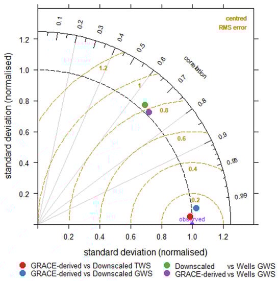
Figure 7.
Taylor diagram showing the correlation coefficients, standard deviations, and root mean square errors (RMSE).
4.4. Performance Analysis of RFM
4.4.1. Spatio-Temporal Variation Characteristics Analysis of TWS
To analyze the consistency of downscaled TWS and GWS on a spatial scale based on RFM, TWS and GWS were compared before and after downscaling. The variations in TWS and GWS were observed in more detail at a higher resolution. Figure 8 represents the spatial variations in TWS and GWS for September 2010. The study area received a series of massive and localized floods in the consecutive years of 2010, 2011, 2012, 2013, 2014, and 2015 [81]. Heavy rainfall of monsoon hit Pakistan at the end of July and September 2010. The rising trend in TWS (Figure 9) after August 2010 played a major role in recharge due to the massive flooding.
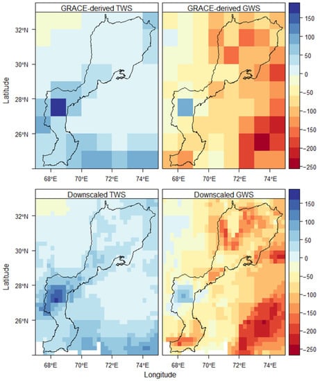
Figure 8.
Original GRACE-derived TWS (mm) and GWS (mm) (upper panel) and RFM downscaled TWS (mm) and GWS (mm) (lower panel).
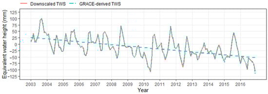
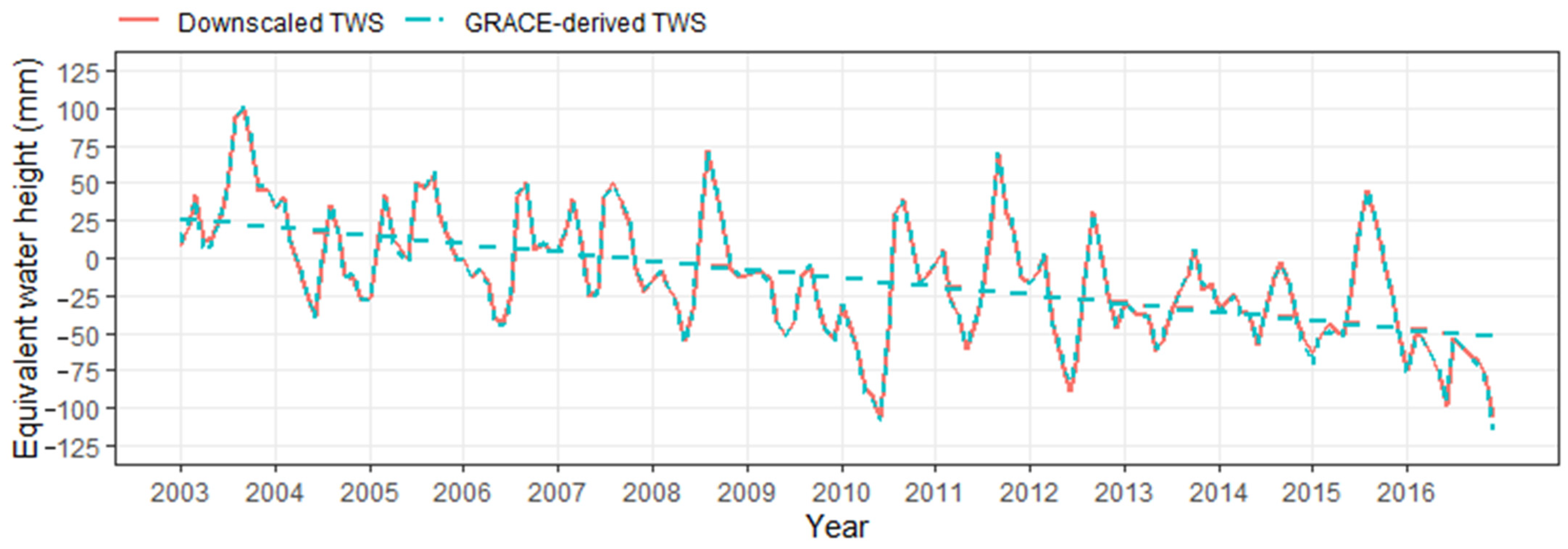
Figure 9.
Terrestrial water storage (TWS) time series before and after downscaling in IBIS.
In Figure 8, the TWS increased near the middle portion, while it decreased in the top left side of the area. While the GWS decreased all over the area except the southwest part of the area. The variations in TWS after downscaling show that the spatial changes can be observed more effectively at a high spatial resolution. Similarly, the variations in GWS after downscaling are observed consistently.
The variability in the trends of GRACE-derived TWS and downscaled TWS is almost the same, showing a declining pattern in the study area. Figure 9 shows variations in the time series of TWS before and after downscaling at low (1°) and high (0.25°) resolution as well as CSR-M TWS, respectively. The variations in amplitude and value of TWS before and after downscaling are consistent (R = 0.99) in the study area. The uncertainty associated with the calculated trend values were calculated from the differences in trend values extracted from the three solutions (CSR, JPL, and GFZ) [82,83]. The GRACE-derived TWS and downscaled TWS is decreasing at the same rate −3.25 ± 0.45 mm/year at a regional scale.
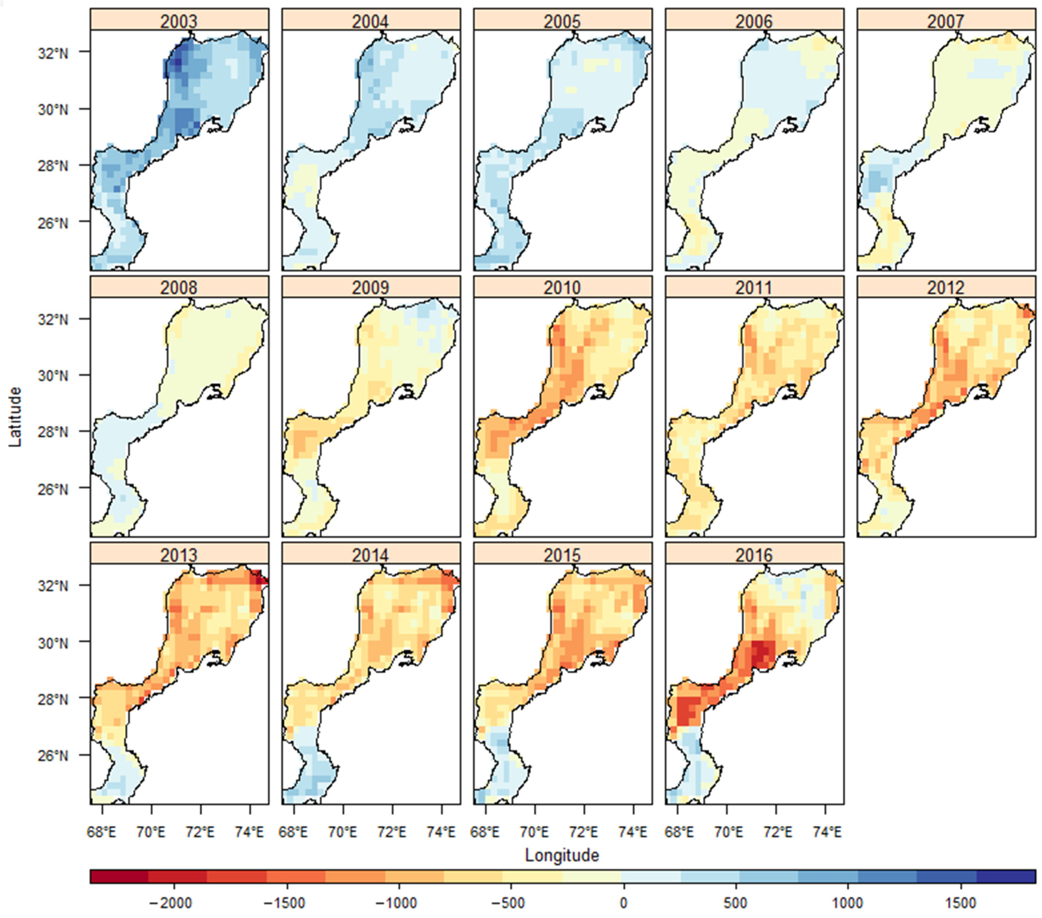
The spatio-temporal maps showing variations in TWS from 2003 to 2016 at a higher resolution on an annual basis are shown in Figure 10 to further demonstrate spatial variability of downscaled RFM results. The IBIS received massive and localized floods due to monsoon rainfall during 2010–2015 in different regions of IBIS. The high amplitude of TWS between August and September during these flooded years can be observed in Figure 9 with high and small peaks. The overall yearly change in TWS at a spatial scale during the flooded year was mostly observed in the lower part of IBIS.
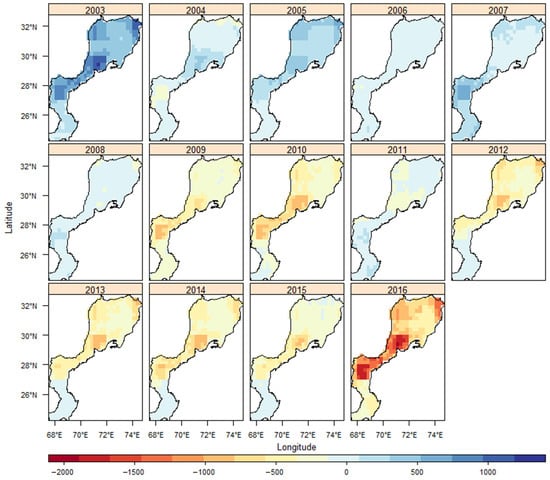
Figure 10.
Spatial distribution of TWS anomaly (mm) on a yearly basis.
4.4.2. Spatio-Temporal Variation Characteristics Analysis of GWS
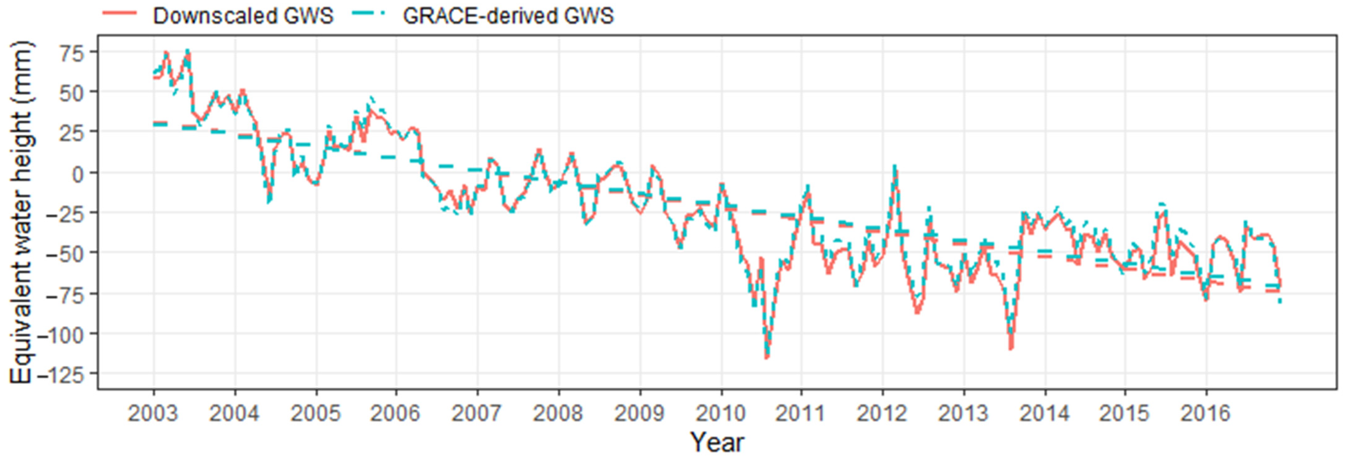
The variations in the trend of GRACE-derived GWS and downscaled GWS showing a declining pattern consistently in the IBIS. Figure 11 shows the variability in the time series of GWS before and after downscaling at low (1°) and high (0.25°) resolution, respectively. The variability of trend in GWS before and after downscaling is consistent, showing R (0.99) in the IBIS (Figure 11). The GRACE-derived GWS and downscaled GWS is decreasing at the same rate −3.39 ± 0.45 mm/year at the regional scale. Table 2 shows the trend variability of downscaled GWS within the study area at a confidence level of 5%.
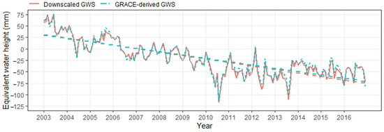
Figure 11.
GWS time series before and after downscaling in IBIS.
Table 2.
Trend and volumetric calculation of GWS.
The yearly spatial downscaled GWS maps were generated at a high resolution from 2003–2016 within the IBIS (Figure 12). The overall spatial distribution of downscaled GWS was similar to that of the TWS, that is, in decreasing trend. Moreover, the sub-grid heterogeneity was captured by downscaled GWS effectively, which is the effect of a local-scale hydro-climatological and geospatial characteristics on GWS. Higher groundwater depletion at the spatial scale was observed comparatively at the end of 2016 in the IBIS (Figure 12). The yearly GWS represents the changes in groundwater abstraction and recharges impacted by climatic variations and anthropogenic activities. The change in the GWS is observed significantly in IBIS from 2003 to 2016 (Figure 12).
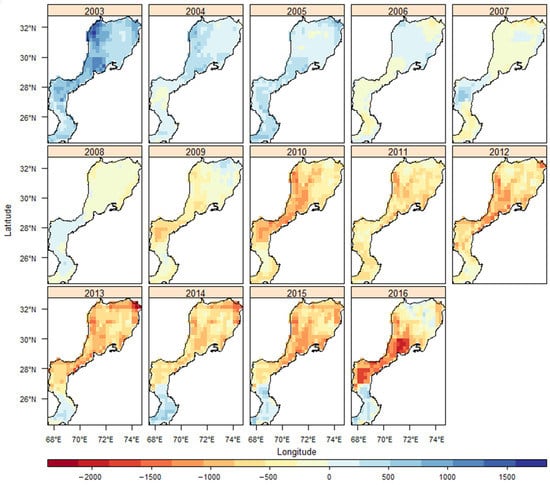
Figure 12.
Spatial distribution of GWS (mm) on a yearly basis.
The supply of canal water was not adequate to fulfill the crop water requirements. This shortage of water was covered through groundwater irrigation. The overexploitation of groundwater was observed in the province of Punjab, which is the upper part of the IBIS as can be seen in the above figure. Iqbal et al. [16] estimated the total loss of about 11.83 km3/year groundwater storage in the upper Indus plain of Punjab province of Pakistan from 2003 to 2010. Tang et al. [15] observed that the groundwater depletion rate is −0.3 ± 0.2 cm/year from 1980 to 2015 in the Punjab province of Pakistan. Irrigation in paddy fields with insufficient canal water supply may be the cause of groundwater abstraction. It is a normal practice to use groundwater in combination with surface water in the Punjab province, Pakistan. The abstraction of groundwater was fragmented because of the poor quality of groundwater in the Sindh province. Nevertheless, percolation from canals and fields replenishes groundwater resulted in the use of groundwater in combination to surface water in the north portion of Sindh [84]. The negative change in GWS (from 2009–2016) is caused by the over-abstraction of groundwater. The spatial patterns of GWS showed that the upper part of the IBIS is under severe groundwater depletion. Whereas, groundwater depletion varies from moderate to severe in the lower part of the IBIS. The spatial variations in GWS can be utilized to find the regions with excessive groundwater depletion for developing groundwater management strategies. Cheema et al. [43] also observed the highest gross groundwater abstraction in the middle and upper parts of the irrigated areas of the Indus basin for the year 2007. The groundwater resources have a relatively good quality of groundwater in these areas [85]. They are present in the Punjab province, Pakistan, and the Indian states of Haryana and Punjab.
The overexploitation of groundwater was also observed in the Indian states of Haryana and Punjab [43]. An assessment of groundwater abstractions showed that the Indian states’ (i.e., Haryana, Punjab, and Rajasthan) loss of groundwater was about 109 km3 from 2002 to 2008 with the water table declining by 17.7 km3/year [1]. While Tiwari et al. [86] observed a loss of about 54 ± 9 km3/year of groundwater storage in northern India. The overexploitation of groundwater at this alarming rate could potentially alter the transboundary groundwater flow between Pakistan and India [87]. Further study of the IBIS using high-resolution models could be complemented to help in understanding the losing or gaining GWS in certain regions.
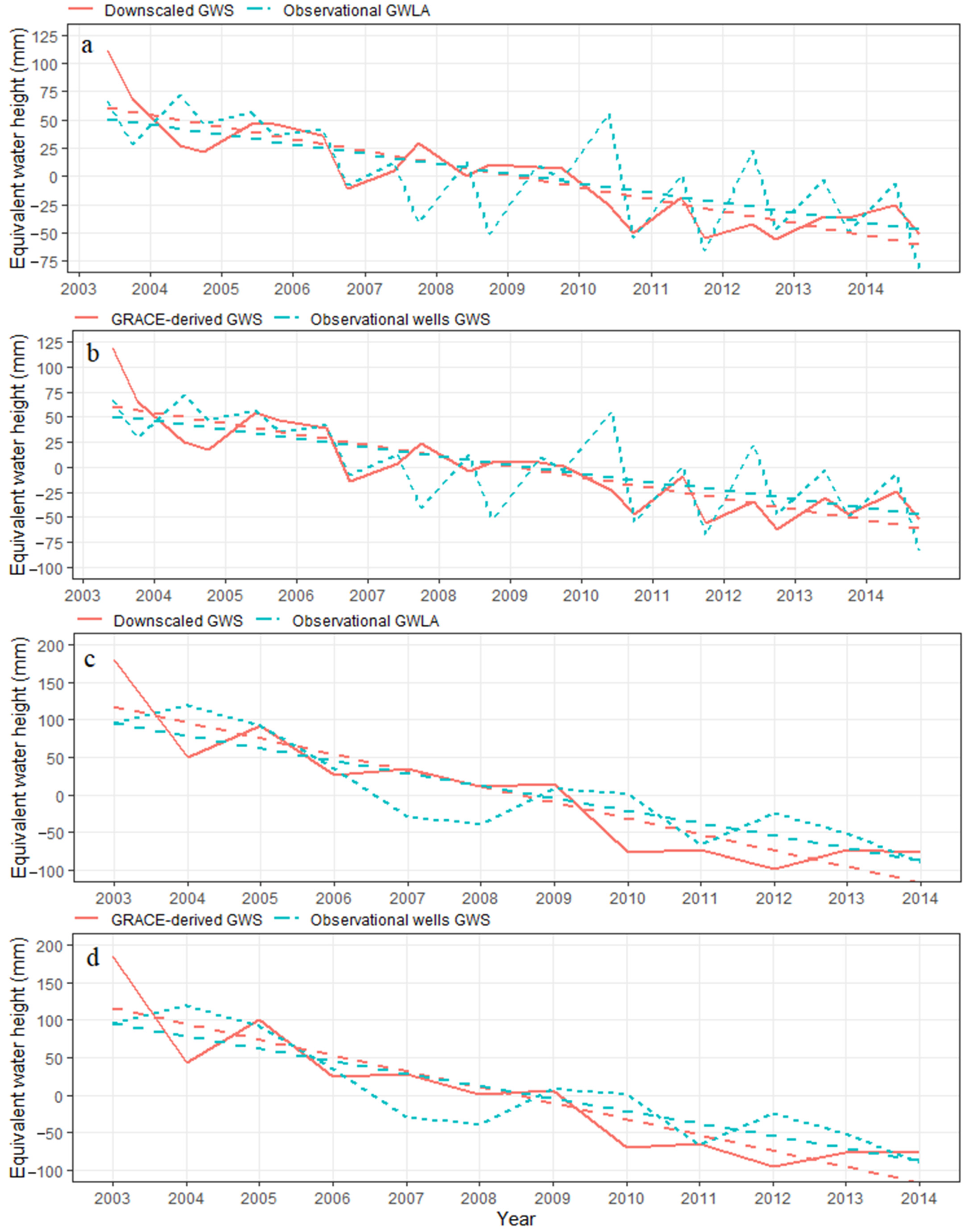
4.4.3. Temporal Validation of Groundwater Storage
The non-uniform distribution of the specific yield is due to heterogeneity in aquifer layers; therefore, GWS estimation becomes more complex. The downscaled GWS was validated with 398 observational wells GWS temporally to assess the performance of downscaling. The temporal variation in GWS was illustrated by overlaying the observational wells on the downscaled GWS. The pixels having observation wells were only selected for validation analysis (Figure 2). Figure 13 shows a comparison of observational wells GWS against downscaled GWS and GRACE-derived GWS on a seasonal and annual scale in the upper part of the IBIS. The observational wells, downscaled, and GRACE-derived GWS show a decreasing trend temporally. The observational wells and downscaled GWS showing a correlation coefficient (R) on a seasonal and annual scale is 0.67 and 0.77, respectively. While GRACE-derived GWS showed correlation (R) is 0.70 and 0.79 in comparison to observational wells GWS on a seasonal and annual scale, respectively. It shows that downscaled GWS is significantly well correlated with the observational wells GWS, as the RFM downscaled GWS replicates the observed GWS with a high correlation. Therefore, RFM not only improves the spatial resolution of data but also ensures the accuracy of data.
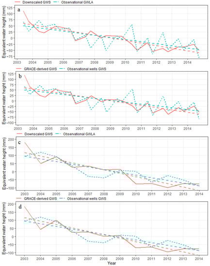
Figure 13.
Comparison of observational wells, downscaled, and GRACE-derived GWS time series (a,b) at the seasonal scale and (c,d) at the annual scale.
5. Discussion
Generally, hydrological products at a higher resolution are a hot topic. In this study, GRACE TWS and GWS were downscaled from 1° to 0.25° by using RFM, which provided an extra research opportunity regarding the data of GRACE. The overall outcomes of RFM downscaled data showed the potential of implement in this type of study. The downscaled GWS was validated with only 398 observational wells data because of the limitation of groundwater level data. In addition, the network of observational wells was not distributed in the entire study area, which causes less influence of heterogeneity and also validates the results less reliable. However, if there were more groundwater level data, this might cause maximum reliability. In the IBIS, extreme spatio-temporal variability in evapotranspiration (ET) due to a large amount of water exploration for agricultural production can make the GLDAS NOAH model estimated ET prone to errors, because GLDAS is an off-satellite model and cannot replicate these effects. Therefore, the uncertainties associated with monthly ET input data may also lead to biases in the statistical model’s estimations.
Nevertheless, the suitability of the downscaling TWS and GWS based on RFM has been provided in this study, which could be utilized in other areas. The applicability of data scarcity regions with limited hydrological variables can be improved using satellite data, for example, groundwater observational wells data with the irregular temporal and spatial distribution. Although, the data from different sources also significantly contribute to uncertainties. For example, there is a presence of an associated uncertainty with the GRACE and input data, which can trigger some propagation of potential errors in cumulative input data [27]. Here, three GRACE satellite spherical harmonic products (CSR, JPL, GFZ) were employed to minimize the uncertainty. These products were multiplied with the scaling coefficients to restore the signals removed by Gaussian, de-striping, and filters (degree 60) of land grids, but there might be uncertainties in the hydrological model at the interannual level. In subsequent research, the researchers can directly estimate the grid at 0.25° × 0.25° using GRACE spherical harmonic coefficients and compare the results of multiple downscaling machine-learning models. At the same time, unavoidable systematic uncertainty in the training of machine-learning models still remains. This study compared the results of two machine-learning models (RFM, ANN). The results showed that the RFM is the best. It shows that RFM is not easily overfitted, and the noise immunity ability is better than ANN. The RFM mitigated these errors because it can handle errors associated with input data.
The possible advantage of downscaling of RFM is that multiple variables can be input simultaneously, which also increases the model’s flexibility. In the model, input variables are independent of each other at the same time, and different variable factors might be preferred for different regions. The regional water management policymaker primarily focuses on GWS at a small scale of the region as compared to the GRACE-derived GWS at a large scale. This coarse resolution problem can be solved effectively by using RFM. It provides more comprehensive information for water decision makers.
The proposed models could be further modified by improving the following aspects in the forthcoming studies. For example, (1) the average of each zone exhibits that tropical rainfall in the tropics directs the TWS fluctuations; however, the evapotranspiration is very much effective in the middle of the latitudes [88]. Hence, considering the latitude of the region, the remote sensing datasets with high resolution can be chosen and utilized for future experimental analysis. The local economic effects and demographic environments must be considered accurately for water reserves, (2) the variables, for example, NDVI, soil types, and many other conditioning factors, can be involved for studying the differential salient features of the current study area, (3) the products with highly remote sensing and fine resolution can be selected for future research goals at a small regional scale to accomplish the provisions of water managers at the regional level.
Comparison of Current and Previously Related Studies
The validation analysis part is constrained due to the data scarcity of observational wells. The independent variables utilized in RFM also had uncertainties. Moreover, GRACE has some missing months data, which were calculated by interpolation, and this process causes errors during estimation of GWS. An artificial neural network (ANN) approach, which is very much precise through hydrological variables (rainfall and soil moisture), could be utilized in future researches. Furthermore, since GRACE launched in April 2002, it has had latencies from 2 to 6 months causing real-time GWS evaluation at a small scale.
In recent times, downscaling of GRACE data was conducted by Gemitzi and Lakshmi [80] and Miro et al. [19] using the ANN model. Both models performed well with calibration. Though, the first model [80] overestimated the in situ data in the validation part. The other model [19] observed an error of almost 1 m in some regions as compared to the observed GWS data. Meanwhile, Seyoum and Milewski [50] performed an ANN model to predict variables by considering the lag effect. The data of this model poorly exhibit the Pearson’s correlation coefficients by depicting more variations as compared to observed GWS. The ANN model was developed by [89] to downscale GRACE data. The Pearson’s correlation coefficient of the model between predicted and the water balanced derived GWS was 0.64 along with RMSE of 22.50 mm.
Except this, the common statistical method [22] presented relatively better results. The currently proposed RFM output exhibits RMSE of 11.83 mm, and the statistical metrics also strengthen the RFM acceptance, since these metrics indicate a high correlation of coefficient (R) and NSE values as compared to the ANN model (Figure 6) and common statistical method [22]. After improving the resolution of GRACE data at a spatial scale based on the RFM, it efficiently permits the evaluation of TWS and GWS in more details at a small regional scale over the globe.
6. Conclusions
The application of GRACE data provides a new research approach to explore variations in GWS at a large scale. This study used two machine-learning models to conduct downscaling and considers the impact of multiple geospatial and hydrological independent variables on TWS. The results showed that RFM has higher accuracy than the ANN model. Therefore, the downscaling was conducted based on the RFM. The TWS was downscaled from 1° to 0.25° successfully and estimated the GWS at high resolution. VIMP illustrates that soil moisture and RF have a relatively higher influence on the downscaling process of RFM. ET and Qs were less sensitive in the downscaling process, even though they are important components of the TWS cycle. The downscaling RFM could predict the variations in water storage at a regional scale relative to long time series very well. The RFM prediction results are ideal in the IBIS. The downscaling model error is very small, and variations in the trend of water storage are consistent before and after downscaling. The sub-grid heterogeneity in spatial variations was captured effectively after downscaling of TWS and GWS, which cannot be comprehended at low resolution.
The observed groundwater level data compared with the downscaled and GRACE-derived GWS data showing the correlation coefficients of 0.67 and 0.77 on the seasonal and annual scale, where it was 0.70 and 0.79 before downscaling. Therefore, RFM can not only improve the spatial resolution but also ensure the accuracy of the data. The quality of downscaled GWS is that it captures the sub-grid heterogeneity effectively and is consistent with the GRACE-derived GWS in the study area on a temporal scale. Therefore, the areas with less density of in situ data can be monitored more accurately by improving the spatial resolution of GWS data. The recently developed RFM allows for the assessment variations in GWS on a spatial scale due to climatic and anthropogenic activities in more detail. It has been observed that RFM can not only increase the spatial resolution of the data effectively but also ensure the accuracy of the data. This study mainly focuses on the downscaling method, and some limitations are present, including the influences of NDVI, as the study area is highly irrigated, anthropogenic activities in the variations of groundwater storages, and the lack of observational wells data in validation section in the IBIS, which will be further investigated and fully evaluated in the near future.
Author Contributions
Conceptualization, S.A.; methodology, S.A.; validation, S.A.; formal analysis, S.A.; investigation, S.A., D.L. and Q.F.; resources, D.L.; data curation, S.A. and M.M.R.; writing—original draft preparation, S.A.; writing—review and editing, D.L., Q.B.P., T.D.D., D.T.A. and M.J.M.C.; visualization, S.A., D.L., T.D.D., D.T.A. and M.J.M.C.; supervision, D.L.; project administration, D.L.; funding acquisition, D.L. All authors have read and agreed to the published version of the manuscript.
Funding
This study research is supported by the National Key R&D Program of China (No.2017YFC0406002), National Natural Science Foundation of China (No.51579044, No.41071053), National Science Fund for Distinguished Young Scholars (No.51825901), Natural Science Foundation of Heilongjiang Province (No. E2017007).
Institutional Review Board Statement
Not applicable.
Informed Consent Statement
Not applicable.
Data Availability Statement
The observed groundwater level data were obtained from the Punjab Irrigation and Drainage Authority (PIDA), which can be downloaded from https://irrigation.punjab.gov.pk/ (accessed on 23 December 2020). Gravity recovery and climate experiment (GRACE) monthly mass grids (RL-05, level-3) processed at Center for Space Research (CSR, the University of Texas), Jet Propulsion Laboratory (JPL, Pasadena, CA, USA), and GeoForschungsZentrum Potsdam (GFZ, Potsdam, Germany) were downloaded from https://grace.jpl.nasa.gov/data/get-data/monthly-mass-grids-land/ (accessed on 13 September 2019). Global land data assimilation system (GLDAS) Noah model products were downloaded from https://disc.gsfc.nasa.gov/datasets (accessed on 23 November 2019). The monthly TRMM 3B43 product Version 7 were downloaded from http://disc. sci.gsfc.nasa.gov/precipitation/ (accessed on 05 October 2019). The Digital Elevation model (DEM) was derived from Shuttle Radar Topographic Mission (SRTM).
Acknowledgments
The financial support is highly appreciated. The authors would like to thank GRACE Tellus for providing the GRACE Tellus land grids data supported by the NASA Measures Program. The GLDAS data used in this study are acquired as part of the mission of NASA’s Earth Science Division and archived and distributed by the Goddard Earth Sciences (GES) Data and Information Services Center (DISC). We appreciate the editors and the reviewers for their constructive suggestions and insightful comments, which helped us greatly to improve this manuscript.
Conflicts of Interest
The authors declare no conflict of interest.
Abbreviations
| GRACE | Gravity Recovery and Climate Experiment |
| TWS | Terrestrial water storage |
| GWS | Groundwater storage |
| RFM | Random forest model |
| IBIS | Indus basin irrigation system |
| DEM | Digital elevation model |
| RMSE | Root mean square error |
| MAE | Mean square error |
| NSE | Nash–Sutcliffe efficiency |
| ET | Evapotranspiration |
| RF | Rainfall |
| SM | Soil moisture |
| Qs | Surface runoff |
| CW | Canopy water |
| CSR | Center for Space Research |
| JPL | Jet Propulsion Laboratory |
| GFZ | GeoForschungsZentrum Potsdam |
| GIA | Glacier isostatic adjustment |
| GLDAS | Global Land Data Assimilation System |
| CLM | Common land model |
| VIC | Variable infiltration capacity |
| GES DISC | Goddard Earth Sciences Data and Information Services Center |
| TRMM | Tropical Rainfall Measuring Mission |
| PIDA | Punjab Irrigation and Drainage Authority |
| DTW | Depth to the water table |
| DTB | Depth to bedrock |
| Groundwater level anomalies | |
| Long-term mean of groundwater level | |
| Groundwater storage anomalies | |
| Specific yield | |
| WBE | Water balance equation |
| CART | Classification and regression decision trees |
| OOB | Out of bag |
| VIMP | Variable importance measure predictive |
| ANN | Artificial neural network |
| NDVI | Normalized difference vegetation index |
| MLP | Multi-layer perceptron |
References
- Rodell, M.; Velicogna, I.; Famiglietti, J.S. Satellite-based estimates of groundwater depletion in India. Nature 2009, 460, 999. [Google Scholar] [CrossRef] [Green Version]
- Wang, Y. The Evaluation of Environmental Quality of Groundwater in Inland Plains—A Study on Yanqi County in Xinjiang. Master’s Thesis, Xinjiang Agricultural University, Urumqi, China, 2010. [Google Scholar]
- Famiglietti, J.S.; Lo, M.; Ho, S.L.; Bethune, J.; Anderson, K.J.; Syed, T.H.; Swenson, S.C.; de Linage, C.R.; Rodell, M. Satellites measure recent rates of groundwater depletion in California’s Central Valley. Geophys. Res. Lett. 2011, 38, L03403. [Google Scholar] [CrossRef] [Green Version]
- Long, D.; Chen, X.; Scanlon, B.R.; Wada, Y.; Hong, Y.; Singh, V.P.; Chen, Y.; Wang, C.; Han, Z.; Yang, W. Have GRACE satellites overestimated groundwater depletion in the Northwest India Aquifer? Sci. Rep. 2016, 6, 24398. [Google Scholar] [CrossRef]
- Ye, S.H.; Huang, C. Space technique monitoring and prediction of groundwater changes. Prog. Geophys. 2007, 4, 1030–1034. (In Chinese) [Google Scholar]
- Ramilliena, G.; Frapparta, F.; Cazenavea, A.; Güntnerb, A. Time variations of land water storage from an inversion of 2 years of GRACE Geoids. Erath Planet. Sci. Lett. 2005, 235, 283–301. [Google Scholar] [CrossRef] [Green Version]
- Davis, J.L.; Elosegui, P.; Mitrovica, J.X. Climate-driven deformation of the solid Earth from GRACE and GPS. Geophys. Res. Lett. 2004, 31, 357–370. [Google Scholar] [CrossRef] [Green Version]
- Yeh, P.J.F.; Swenson, S.C.; Famiglietti, J.S.; Rodell, M. Remote Sensing of groundwater storage changes in Illinois using the Gravity Recovery and Climate Experiment (GRACE). Water Resour. Res. 2006, 42, W05417. [Google Scholar] [CrossRef]
- Rodell, M.; Chen, J.; Kato, H.; Famiglietti, J.S.; Nigro, J.; Wilson, C.R. Estimating groundwater storage changes in the Mississippi River basin (USA) using GRACE. Hydrogeol. J. 2007, 15, 159–166. [Google Scholar] [CrossRef] [Green Version]
- Feng, W.; Zhong, M.; Lemoine, J.; Biancale, R.; Hsu, H.; Xia, J. Evaluation of groundwater depletion in North China using the Gravity Recovery and Climate Experiment (GRACE) data and ground-based measurements. Water Resour. Res. 2013, 49, 2110–2118. [Google Scholar] [CrossRef]
- Castellazzi, P.; Longuevergne, L.; Martel, R.; Rivera, A.; Brouard, C.; Chaussard, E. Quantitative mapping of groundwater depletion at the water management scale using a combined GRACE/InSAR approach. Remote Sens. Environ. 2018, 205, 408–418. [Google Scholar] [CrossRef]
- Swenson, S.; Wahr, J.; Milly, P.C.D. Estimated accuracies of regional water storage variations inferred from the Gravity Recovery and Climate Experiment (GRACE). Water Resour. Res. 2003, 39, 1121–1134. [Google Scholar] [CrossRef]
- Scanlon, B.R.; Longuevergne, L.; Long, D. Ground referencing GRACE satellite estimates of groundwater storage changes in the California Central Valley, USA. Water Resour. Res. 2012, 48, W04520. [Google Scholar] [CrossRef] [Green Version]
- Richey, A.S.; Thomas, B.F.; Lo, M.; Reager, J.T.; Famiglietti, J.S.; Voss, K.; Swenson, S.; Rodell, M. Quantifying renewable groundwater stress with GRACE. Water Resour. Res. 2015, 52, 4184–4187. [Google Scholar] [CrossRef] [PubMed]
- Tang, Y.; Hooshyar, M.; Zhu, T.; Ringler, C.; Sun, A.Y.; Long, D.; Wang, D. Reconstructing annual groundwater storage changes in a large-scale irrigation region using GRACE data and Budyko model. J. Hydrol. 2017, 551, 397–406. [Google Scholar] [CrossRef]
- Iqbal, N.; Hossain, F.; Lee, H.; Akhter, G. Satellite Gravimetric Estimation of Groundwater Storage Variations Over Indus Basin in Pakistan. IEEE J. Sel. Top. Appl. Earth Obs. Remote Sens. 2016, 9, 3524–3534. [Google Scholar] [CrossRef]
- Liu, C.M.; Liu, W.B.; Fu, G.B.; OuYang, R.L. A discussion of some aspects of statistical downscaling in climate impacts assessment. Adv. Water Sci. 2012, 23, 427–437. (In Chinese) [Google Scholar]
- Alley, W.M.; Konikow, L.F. Bringing GRACE Down to Earth. Ground Water 2015, 53, 826–829. [Google Scholar] [CrossRef]
- Miro, M.E.; Famiglietti, J.S. Downscaling GRACE Remote Sensing Datasets to High-Resolution Groundwater Storage Change Maps of California’s Central Valley. Remote Sens. 2018, 10, 143. [Google Scholar] [CrossRef] [Green Version]
- Zhang, M.Y.; Peng, D.Z.; Hu, L.J. Research Progress on Statistical Downscaling Methods. South-to-North South-to-North Water Transf. Water Sci. Technol. 2013, 11, 118–122. (In Chinese) [Google Scholar]
- Liu, Y.H.; Guo, W.D.; Feng, J.M.; Zhang, K.X. A Summary of Methods for Statistical Downscaling of Meteorological Data. Adv. Earth Sci. 2011, 26, 837–847. (In Chinese) [Google Scholar]
- Ning, S.W.; Ishidaira, H.; Wang, J. Statistical downscaling of GRACE-derived terrestrial water storage using satellite and GLDAS products. J. Jpn. Soc. Civ. Eng. 2014, 70, 133–138. [Google Scholar] [CrossRef]
- Yin, W.; Hu, L.; Zhang, M.; Wang, J.; Han, S.C. Statistical Downscaling of GRACE-Derived Groundwater Storage Using ET Data in the North China Plain. J. Geophys. Res. Atmos. 2018, 123, 5973–5987. [Google Scholar] [CrossRef]
- Chen, S.; She, D.; Zhang, L.; Guo, M.; Liu, X. Spatial Downscaling Methods of Soil Moisture Based on Multisource Remote Sensing Data and Its Application. Water 2019, 11, 1401. [Google Scholar] [CrossRef] [Green Version]
- Li, W.; Ni, L.; Li, Z.; Duan, S.; Wu, H. Evaluation of Machine Learning Algorithms in Spatial Downscaling of MODIS Land Surface Temperature. IEEE J. Sel. Top. Appl. Earth. Obs. Remote Sens. 2019, 12, 2299–2307. [Google Scholar] [CrossRef]
- Shi, Y.; Song, L.; Xia, Z.; Lin, Y.; Myneni, R.B.; Choi, S.; Wang, L.; Ni, X.; Lao, C.; Yang, F. Mapping Annual Precipitation across Mainland China in the Period 2001–2010 from TRMM3B43 Product Using Spatial Downscaling Approach. Remote Sens. 2015, 7, 5849–5878. [Google Scholar] [CrossRef] [Green Version]
- Seyoum, W.M.; Kwon, D.; Milewski, A.M. Downscaling GRACE TWSA data into High-Resolution Groundwater Level Anomaly Using Machine Learning-Based Models in a Glacial Aquifer System. Remote Sens. 2019, 11, 824. [Google Scholar] [CrossRef] [Green Version]
- Rahaman, M.M.; Thakur, B.; Kalra, A.; Ahmad, S. Modeling of GRACE-Derived Groundwater Information in the Colorado River Basin. Hydrology 2019, 6, 19. [Google Scholar] [CrossRef] [Green Version]
- Sun, A.Y. Predicting groundwater level changes using GRACE data. Water Resour. Res. 2013, 49, 5900–5912. [Google Scholar] [CrossRef]
- Yang, P.; Xia, J.; Zhan, C.; Wang, T. Reconstruction of terrestrial water storage anomalies in Northwest China during 1948–2002 using GRACE and GLDAS products. Hydrol. Res. 2018, 49, 1594–1607. [Google Scholar] [CrossRef] [Green Version]
- Li, B.; Rodell, M.; Zaitchik, B.F.; Reichle, R.H.; Koster, R.D.; van Dam, T.M. Assimilation of GRACE terrestrial water storage into a land surface model: Evaluation and potential value for drought monitoring in western and central Europe. J. Hydrol. 2012, 446, 103–115. [Google Scholar] [CrossRef] [Green Version]
- Schmidt, R.; Schwintzer, P.; Flechtner, F.; Reigber, C.; Guntner, A.; Doll, P.; Ramillien, G.; Cazenave, A.; Petrovic, S.; Jochmann, H.; et al. GRACE observations of changes in continental water storage. Glob. Planet. Chang. 2006, 50, 112–126. [Google Scholar] [CrossRef]
- Chen, L.; He, Q.; Liu, K.; Li, J.; Jing, C. Downscaling of GRACE-Derived Groundwater Storage Based on the Random Forest Model. Remote Sens. 2019, 11, 2979. [Google Scholar] [CrossRef] [Green Version]
- Zhang, J.; Liu, K.; Wang, M. Downscaling Groundwater Storage Data in China to a 1-km Resolution Using Machine Learning Methods. Remote Sens. 2021, 13, 523. [Google Scholar] [CrossRef]
- Reager, J.T.; Famiglietti, J.S. Characteristic mega-basin water storage behaviour using GRACE. Water Resour. Res. 2013, 49, 3314–3329. [Google Scholar] [CrossRef] [PubMed] [Green Version]
- World Commission on Dams (WCD). Tarbela Dam and Related Aspects of the Indus River Basin in Pakistan; WCD: New Delhi, India, 2000. [Google Scholar]
- Ojeh, E. Hydrology of the Indus Basin (Pakistan). 2006. Available online: https://cupdf.com/document/hydrology-of-the-indus-basin-pakistan-gis-term-project-by-elizabeth-ojeh-30.html (accessed on 31 August 2021).
- Habib, Z. Scope for Reallocation of Rivers Waters for Agriculture in the Indus Basin. Ph.D. Thesis, Environmental Sciences, Spécialité Sciences de l‘Eau, ENGREF, Paris, France, 2004. [Google Scholar]
- Ullah, M.K.; Habib, Z.; Muhammad, S. Spatial Distribution of Reference and Potential Evapotranspiration across the Indus Basin Irrigation Systems; IWMI working paper; IWMI: Lahore, Pakistan, 2001; Volume 24. [Google Scholar]
- PBS. Pakistan Statistical Yearbook; PBS: Boston, MA, USA, 2014. [Google Scholar]
- Watto, M.A.; Mugera, A.W. Groundwater depletion in the Indus Plains of Pakistan: Imperatives, repercussions and management issues. Int. J. River Basin Manag. 2016, 14, 447–458. [Google Scholar] [CrossRef]
- Mekonnen, D.; Siddiqi, A.; Ringler, C. Drivers of groundwater use and technical efficiency of groundwater, canal water, and conjunctive use in Pakistan’s Indus irrigation system. Int. J. Water Resour. Dev. 2015, 627, 459–476. [Google Scholar]
- Cheema, M.J.M.; Immerzeel, W.W.; Bastiaanssen, W.G.M. Spatial quantification of groundwater abstraction in the irrigated Indus basin. Groundwater 2014, 52, 25–36. [Google Scholar] [CrossRef] [Green Version]
- Iqbal, N.; Hossain, F.; Lee, H.; Akhter, G. Integrated groundwater resource management in Indus Basin using satellite gravimetry and physical modeling tools. Environ. Monit. Assess. 2017, 189, 128. [Google Scholar] [CrossRef]
- Ahmad, S. Keynote Address, paper presented to national conference on “Water shortage and future agriculture in Pakistan—Challenges and opportunities”. In Proceedings of the National Conference Organized by the Agriculture Foundation of Pakistan, Islamabad, Pakistan, 26–27 August 2008. [Google Scholar]
- Ahmad, S. Scenarios of surface and groundwater availability in the Indus Basin Irrigation System (IBIS) and planning for future agriculture. In Paper Contributed to the Report of the Sub-Committee on Water and Climate Change Task Force on Food Security; Planning Commission of Pakistan: Karachi, Pakistan, 2008. [Google Scholar]
- Qureshi, A.S.; McCornick, P.G.; Qadir, M.; Aslam, Z. Managing salinity and waterlogging in the Indus Basin of Pakistan. Agric. Water Manag. 2008, 95, 1–10. [Google Scholar] [CrossRef]
- Landerer, F.W.; Swenson, S.C. Accuracy of scaled GRACE terrestrial water storage estimates. Water Resour. Res. 2012, 48, W04531. [Google Scholar] [CrossRef]
- Wahr, J.; Molenaar, M.; Bryan, F. Time variability of the Earth’s gravity field: Hydrological and oceanic effects and their possible detection using GRACE. J. Geophys. Res. Solid Earth 1998, 103, 30205–30229. [Google Scholar] [CrossRef]
- Seyoum, W.M.; Milewski, A.M. Improved methods for estimating local terrestrial water dynamics from grace in the northern high plains. Adv. Water Resour. Res. 2017, 110, 279–290. [Google Scholar] [CrossRef]
- Long, D.; Yang, Y.; Wada, Y.; Hong, Y.; Liang, W.; Chen, Y. Deriving scaling factors using a global hydrological model to restore GRACE total water storage changes for China’s Yangtze River Basin. Remote Sens. Environ. 2015, 168, 177–193. [Google Scholar] [CrossRef]
- Rodell, M.; Houser, P.; Jambor, U.; Gottschalck, J.; Mitchell, K.; Meng, C.-J.; Arsenault, K.; Cosgrove, B.; Radakovich, J.; Bosilovich, M. The global land data assimilation system. Bull. Am. Meteorol. Soc. 2004, 85, 381–394. [Google Scholar] [CrossRef] [Green Version]
- Wang, W.; Cui, W.; Wang, X.; Chen, X. Evaluation of GLDAS-1 and GLDAS-2 forcing data and Noah model simulations over China at monthly scale. J. Hydrol. 2016, 17, 2815–2833. [Google Scholar] [CrossRef]
- Dinku, T.; Ceccato, P.; Grover-Kopec, E.; Lemma, M.; Connor, S.J.; Ropelewski, C.F. Validation of satellite rainfall products over East Africa’s complex topography. Int. J. Remote Sens. 2007, 28, 1503–1526. [Google Scholar] [CrossRef]
- Karaseva, M.O.; Prakash, S.; Gairola, R.M. Validation of high-resolution TRMM- B43 precipitation product using rain gauge measurements over Kyrgyzstan. Theor. Appl. Climatol. 2011, 108, 147–157. [Google Scholar] [CrossRef]
- Duan, Z.; Bastiaanssen, W.G.M.; Liu, J. Monthly and annual validation of TRMM Multisatellite Precipitation Analysis (TMPA) products in the Caspian Sea Region for the period 1999–2003. In Geoscience and Remote Sensing Symposium (IGARSS); IEEE International: Piscatway, NJ, USA, 2012; pp. 3696–3699. [Google Scholar]
- Ji, X.; Chen, Y. Characterizing spatial patterns of precipitation based on corrected TRMM 3B43 data over the mid Tianshan Mountains of China. J. Mt. Sci. 2012, 9, 628–645. [Google Scholar] [CrossRef]
- Cheema, M.J.M.; Bastiaanssen, W.G.M. Local calibration of remotely sensed rainfall from the TRMM satellite for different periods and spatial scales in the Indus Basin. Int. J. Remote Sens. 2012, 33, 2603–2627. [Google Scholar] [CrossRef]
- Sun, A.Y.; Green, R.; Rodell, M.; Swenson, S. Inferring aquifer storage parameters using satellite and in situ measurements: Estimation under uncertainty. Geophys. Res. Lett. 2010, 37, L10603. [Google Scholar] [CrossRef] [Green Version]
- Strassberg, G.; Scanlon, B.R.; Rodell, M. Comparison of seasonal terrestrial water storage variations from GRACE with groundwater-level measurements from the High Plains Aquifer (USA). Geophys. Res. Lett. 2007, 34, L14402. [Google Scholar] [CrossRef] [Green Version]
- Greenman, D.W.; Swarzenski, W.V.; Bennett, G.D. Ground-Water Hydrology of the Punjab, West Pakistan, with Emphasis on Problems Caused by Canal Irrigation; US Government Printing Office: Washington, DC, USA, 1967.
- Sridhar, V.; Wedin, D.A. Hydrological behavior of Grasslands of the Sandhills: Water and Energy Balance Assessment from Measurements, Treatments and Modeling. Ecohydrology 2009, 2, 195–212. [Google Scholar] [CrossRef]
- Mann, H.B. Nonparametric tests against trend. Econom. J. Econom. Soc. 1945, 13, 245–259. [Google Scholar] [CrossRef]
- Kendall, M.G. Rank Correlation Measures, 4th ed.; Charles Griffin: London, UK, 1975. [Google Scholar]
- Zolfaghari, A.; Izadi, M. Burst Pressure Prediction of Cylindrical Vessels Using Artificial Neural Network. J. Press. Vessel Technol. 2020, 142, 031303. [Google Scholar] [CrossRef]
- Gholami, V.; Booij, M.J.; Nikzad Tehrani, E.; Hadian, M.A. Spatial Soil Erosion Estimation Using an Artificial Neural Network (ANN) and Field Plot Data. Catena 2018, 163, 210–218. [Google Scholar] [CrossRef]
- Mohaghegi, S.; Del Valle, Y.; Venayagamoorthy, G.K.; Harley, R.G. A Comparison of PSO and Backpropagation for Training RBF Neural Networks for Identification of a Power System with Statcom. In Proceedings of the 2005 IEEE Swarm Intelligence Symposium, Pasadena, CA, USA, 8–10 June 2005; pp. 391–394. [Google Scholar]
- Turban, E.; Sharda, R.; Aronson, J.E.; King, D.N. Business Intelligence: A Managerial Approach; Pearson Prentice Hall: Upper Saddle River, NJ, USA, 2008. [Google Scholar]
- Howitt, R.; MacEwan, D.; Medellín-Azuara, J.; Lund, J.; Sumner, D. Economic Analysis of the 2015 Drought for California Agriculture; UC Davis Center for Watershed Science: Davis, CA, USA, 2015. [Google Scholar]
- Lo, M.; Famiglietti, J.S. Irrigation in California’s Central Valley strengthens the southwestern U.S. water cycle. Geophys. Res. Lett. 2013, 40, 301–306. [Google Scholar] [CrossRef] [Green Version]
- MacKay, D. Bayesian Interpolation. Neural. Comput. 1992, 4, 415–447. [Google Scholar] [CrossRef]
- Breiman, L. Random Forest. Mach. Learn. 2001, 45, 5–32. [Google Scholar] [CrossRef] [Green Version]
- Liaw, A.; Wiener, M. Classification and Regression by randomForest. R News 2002, 2, 18–22. [Google Scholar]
- Cutler, D.R.; Edwards, T.C., Jr.; Beard, K.H.; Cutler, A.; Hess, K.T.; Gibson, J.; Lawler, J.J. Random forests for classification in ecology. Ecology 2007, 88, 2783–2792. [Google Scholar] [CrossRef]
- Fukda, S.; Yasunaga, E.; Nagle, M.; Yuge, K.; Sardsud, V.; Spreer, W.; Muller, J. Modelling the relationship between peel colour and the quality of fresh mango fruit using Random Forests. J. Food Eng. 2014, 131, 7–17. [Google Scholar] [CrossRef]
- Zhou, X.; Zhu, X.; Dong, Z.; Guo, W. Estimation of biomass in wheat using random forest regression algorithm and Remote Sensing data. Crop J. 2016, 4, 212–219. [Google Scholar]
- R Core Team. R: A Language and Environment for Statistical Computing; R Foundation for Statistical Computing: Vienna, Austria, 2020; Available online: https://www.R-project.org/ (accessed on 25 December 2020).
- Milewski, A.M.; Thomas, M.B.; Seyoum, W.M.; Rasmussen, T.C. Spatial Downscaling of GRACE TWSA Data to Identify Spatiotemporal Groundwater Level Trends in the Upper Floridan Aquifer, Georgia, USA. Remote Sens. 2019, 11, 2756. [Google Scholar] [CrossRef] [Green Version]
- Sahour, H.; Sultan, M.; Vazifedan, M.; Abdelmohsen, K.; Karki, S.; Yellich, J.A.; Gebremichael, E.; Alshehri, F.; Elbayoumi, T.M. Statistical applications to downscale GRACE-derived terrestrial water storage data and to fill temporal gaps. Remote Sens. 2020, 12, 533. [Google Scholar] [CrossRef] [Green Version]
- Gemitzi, A.; Lakshmi, V. Downscaling GRACE data to estimate groundwater use at the aquifer scale. In Proceedings of the 15th International Conference on Environmental Science and Technology (CEST), Rhodes, Greece, 31 August–2 September 2017. [Google Scholar]
- Rehman, A.; Jingdong, L.; Du, Y.; Khatoon, R.; Wagan, A.S.; Nisar, S.K. Flood Disaster in Pakistan and its Impact on Agriculture Growth (A Review). Glob. Adv. Res. J. Agric. Sci. 2015, 4, 827–830. [Google Scholar]
- Rodell, M.; Famiglietti, J.S.; Wiese, D.N.; Reager, J.T.; Beaudoing, H.K.; Landerer, F.W.; Lo, M.H. Emerging Trends in Global Freshwater Availability. Nature 2018, 557, 651–659. [Google Scholar] [CrossRef] [PubMed]
- Scanlon, B.R.; Zhang, Z.; Save, H.; Sun, A.Y.; Schmied, H.M.; Van Beek, L.P.H.; Wiese, D.N.; Wada, Y.; Long, D.; Reedy, R.C.; et al. Global Models Underestimate Large Decadal Declining and Rising Water Storage Trends Relative to GRACE Satellite Data. Proc. Natl. Acad. Sci. USA 2018, 115, E1080–E1089. [Google Scholar] [CrossRef] [PubMed] [Green Version]
- Siebert, S.; Doll, P. Quantifying blue and green virtual water contents in global crop production as well as potential production losses without irrigation. J. Hydrol. 2010, 384, 198–217. [Google Scholar] [CrossRef]
- Arshad, M.; Cheema, M.J.M.; Ahmed, S. Determination of lithology and groundwater quality using electrical resistivity survey. Int. J. Agric. Biol. 2007, 9, 143–146. [Google Scholar]
- Tiwari, V.M.; Wahr, J.; Swenson, S. Dwindling groundwater resources in northern India, from satellite gravity observations. Geophys. Res. Lett. 2009, 36, L18401. [Google Scholar] [CrossRef] [Green Version]
- IUCN. Beyond Indus Water Treaty: Ground Water and Environmental Management Policy Issues and Options; IUCN: Karachi, Pakistan, 2010. [Google Scholar]
- Syed, T.H.; Famiglietti, J.S.; Rodell, M.; Chen, J.; Wilson, C.R. Analysis of terrestrial water storage changes from GRACE and GLDAS. Water Resour. Res. 2008, 44, W02433. [Google Scholar] [CrossRef]
- Seo, J.Y.; Lee, S. Spatio-Temporal Groundwater Drought Monitoring Using Multi-Satellite Data Based on an Artificial Neural Network. Water 2019, 11, 1953. [Google Scholar] [CrossRef] [Green Version]


Publisher’s Note: MDPI stays neutral with regard to jurisdictional claims in published maps and institutional affiliations. |
© 2021 by the authors. Licensee MDPI, Basel, Switzerland. This article is an open access article distributed under the terms and conditions of the Creative Commons Attribution (CC BY) license (https://creativecommons.org/licenses/by/4.0/).