Abstract
Lakes are sensitive indicators of climate change in the Tibetan Plateau (TP), which have shown high temporal and spatial variability in recent decades. The driving forces for the change are still not entirely clear. This study examined the area change of the lakes greater than 1 km2 in the endorheic basins of the Tibetan Plateau (EBTP) using Landsat images from 1990 to 2019, and analysed the relationships between lake area and local and large-scale climate variables at different geographic scales. The results show that lake area in the EBTP has increased significantly from 1990 to 2019 at a rate of 432.52 km2·year−1. In the past 30 years, lake area changes in the EBTP have mainly been affected by local climate variables such as precipitation and temperature. At a large scale, Indian Summer Monsoon (ISM) has correlations with lake area in western sub-regions in the Inner Basin (IB). While Atlantic Multidecadal Oscillation (AMO) has a significant connection with lake area, the North Atlantic Oscillation (NAO) does not. We also found that abnormal drought (rainfall) brought by the El Niño/La Niña events are significantly correlated with the lake area change in most sub-regions in the IB.
1. Introduction
The Tibetan Plateau (TP) is known as the “third pole” of the earth. It is also the water tower of Asia [1,2] and is of great significance to regional- and large-scale climate systems due to its large extent and high altitude [3]. Climate in the TP showed a significant increase in temperature and precipitation in most regions over the past decades, especially in the eastern and central parts [4,5]. There are many lakes in the endorheic basins of the Tibetan Plateau (EBTP), which play a special role as they link the atmosphere, cryosphere and biosphere components of the hydrological cycle [6,7]. The lakes are sensitive to climate change, as they respond to the environmental changes in their catchments [8,9]. Besides, glacier, ice and snow cover 17% of the Great Himalayan area and they shrank faster than the world average [10]. Glacier melting and precipitation increase tend to accelerate water cycling and increase the water storage in the TP [4]. As such, lake area change in the region reflects the influence of local climate variables (temperature, precipitation, etc.) and large-scale climate factors (regional monsoon systems, global atmosphere and ocean circulation, etc.), which are of great interest and significance for understanding the hydrological processes in the TP [11,12]. In recent decades, the TP has experienced significant climate change, characterized by unprecedented warming [13], weakening winds [14], reduced potential evaporation [15], precipitation increase [16] and water vapor increase [17]. These changes have severely affected the water cycle in the area, leading to significant changes in lake area in the EBTP [18].
Numerous studies have used optical remote sensing imagery to monitor lake area change in the EBTP over the past decades [1,9,16,17,18,19,20,21,22]. As shown in Table 1, these studies either only focused on some large lakes or only examined lake area in some specific years (every 5 or 10 years) or for a short time span of less than 15 years. Without a long-term annual census, the temporal variation of lake area cannot be well examined, and it is difficult to study the impacts of climate change on lake area at an inter-annual scale. There are some long-term surface water data, such as the Joint Research Centre (JRC) data [23], which contain many types of water and in them it is difficult to separate lakes from other water bodies.

Table 1.
Recent lake studies and related datasets in the TP.
Lakes in the EBTP are not connected to external waterbodies, and they are sensitive to the change of local climate variables [17]. Climate system in the region is quite complex, potentially at the confluence of monsoon systems, including the East Asian Summer Monsoon (EASM) and the Indian Summer Monsoon (ISM), and the westerlies [25]. Previous studies have shown that the ISM may bring precipitation to southeastern and inner TP [26,27] and Chang et al. [28] have shown that the monsoons are related to precipitation in parts of the TP using wavelet and global coherence analysis. However, it is not known whether the EASM and ISM affect the lake area in the EBTP through their impacts on precipitation. Northwestern TP is dominated by the westerlies [25,29,30], which is related to some global atmospheric circulations such as North Atlantic Oscillation (NAO) and Atlantic Multidecadal Oscillation (AMO). In addition, El Niño/La Niña events have also shown close relationship to abnormal drought (rainfall) events in some areas of the TP [31]. However, it is unclear whether the lake area in the EBTP is related to these events through teleconnection.
In this research, using the Google Earth Engine (GEE) geospatial analysis platform, we analyzed Landsat imagery in the past 30 years (1989–2019) to obtain annual lake area time series data for 976 lakes with a maximum area larger than 1 km2 in the endorheic basin of the TP (EBTP). It provides the most comprehensive census on lake area change in the EBTP so far. Based on the data, we explored the relationships between lake area and local and large-scale climate variables at different geographic scales. The research helps us better understand the changes of lake area in the past 30 years and lake response to climate change in the region.
2. Materials and Methods
2.1. Study Area
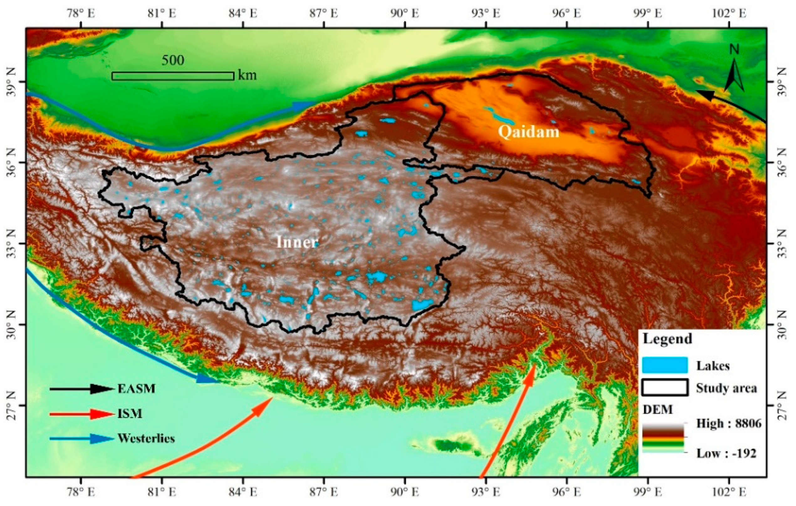
Based on hydro-geomorphology factors, the TP can be divided into 12 sub-watersheds [32]. Our study area includes the Inner Basin (IB) and Qaidam Basin (QB), which are the two major endorheic basins of the TP containing most of the lakes in the TP (Figure 1). The study area is ~1.42 million km2, accounting for 32% of the total area of the TP. The average elevation is 4547 m. According to the lake area data released by the Qinghai-Tibet Plateau Research Institute of the Chinese Academy of Sciences (CAS) [18,33] (Zhang’s data hereafter), the lake area in the IB and QB accounts for 74% of the total lake area in the TP in 2018. As shown in Figure 1, the study area is mainly affected by ISM and westerlies, but with limited impact from the EASM [29].
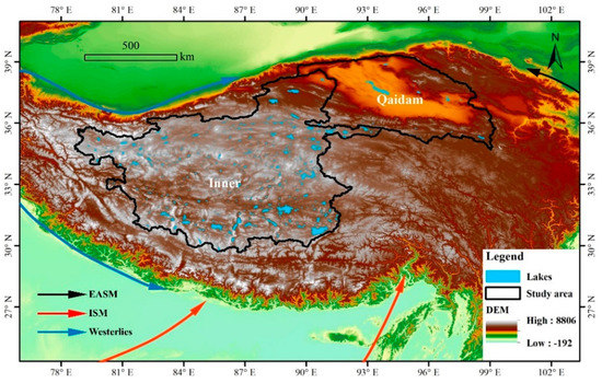
Figure 1.
Study area (the Inner Basin and Qaidam Basin) and the main atmospheric circulations affecting the TP. The circulation paths are re-drawn based on Figure 1 in [29].
To study sub-regional difference in lake area changes and their response to climate change, we divided the study area into 10 sub-regions based on watershed boundary and climate types. According to Köppen climate classification system [34], there are three main climate types in the area (Figure 2): mid-latitude cold desert (BSk), tundra (ET), and temperate cold desert (BWk). We combined the 462 watersheds from HydroSHEDS [35] with the Köppen climate types and delineated 10 sub-regions (Figure 2).
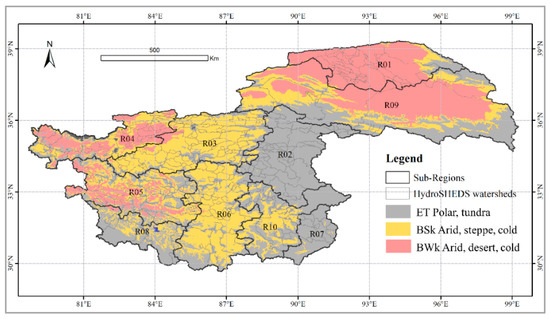
Figure 2.
Ten sub-regions in the study area delineated based on HydroSHEDS watersheds and Köppen climate types.
2.2. Data
2.2.1. Surface Water Data, DEM and Landsat Imagery
The data used in this study include the JRC Global Surface Water Mapping Layers v1.2, SRTM DEM and Landsat images. The JRC data contain global surface water coverage over 1984–2019 and provides statistics on the extent and change of surface water. We used the JRC data to obtain the maximum extent for each lake and the SRTM DEM to remove the rivers connected to lakes. The Landsat images used for mapping annual lake area include Collection 1 Tier 1 raw scenes from Landsat5/7/8 with a resolution of 30 m. In this research, images from Landsat-5 TM (1984–2012), Landsat-7 ETM+ (1999–2019), and Landsat-8 OLI (2013–2019) between 16 March 1984 and 31 December 2019 were used to generate a composite image in each year for each lake. The annual composite images usually represent the maximum lake extent in a year (see Section 2.3.1). All the data were accessed and analyzed on Google Earth Engine [36].
2.2.2. Climate Data
There are several meteorological datasets available for the TP, which are not completely consistent. After comparison, we use the China meteorological forcing dataset [37,38,39] provided by the Qinghai-Tibet Plateau Data Center of the CAS. It is reanalysis data which has a better accuracy than other reanalysis datasets available in the area [37,40]. This gridded dataset has a spatial resolution of 0.1° × 0.1° and temporal resolution of 3 h, and includes seven climate elements. The dataset is in NetCDF format and has been validated with good quality and widely applied in long-term climate change analysis in the TP [37,40]. We extracted annual mean temperature and annual precipitation over 1990–2018 for the EBTP from the dataset and calculated the annual mean temperature and annual precipitation for each sub-region for the same time period.
To study the connection between lake area and regional atmospheric circulations such as monsoon systems, we used two major Asian monsoon indices: the ISM index, which is the normalized anomalies of sea level pressure (SLP) difference between the Indian sea zone (40°E–80°E, 5°N–15°N) and central Asia (70°E–90°E, 20°N–30°N) [41], and the EASM Index, which is defined as the area-averaged dynamical normalized seasonality at 850 hPa within the domain of (10°N–40°N, 110°E–140°E) [42]. The summer monsoons are pronounced in warm seasons, and therefore only summer season composites [25] were examined.
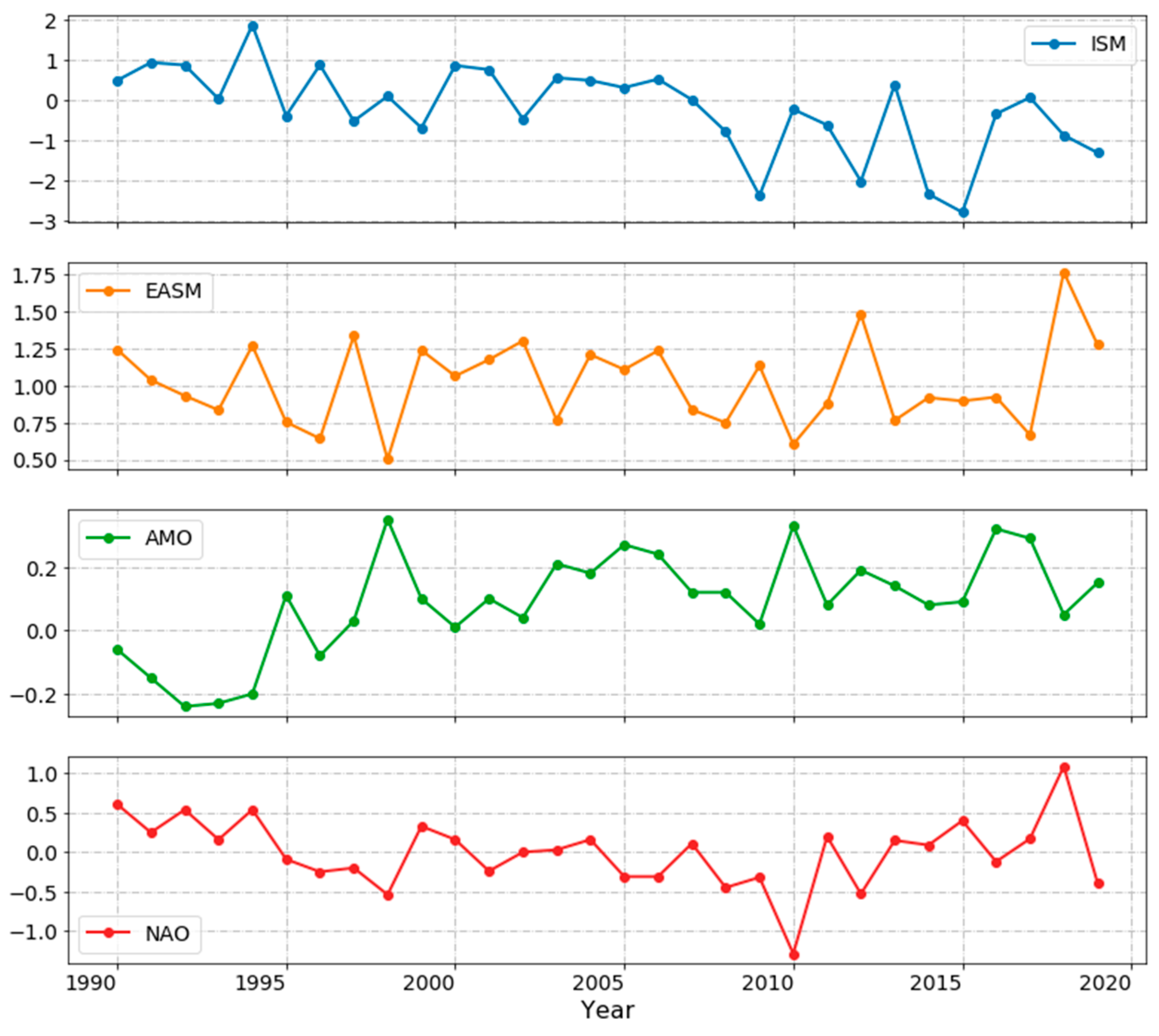
In addition to monsoon indices, several global circulation indices are also used in this study. The AMO index [43], a ten-year running mean of detrended Atlantic sea surface temperature anomaly north of the equator, is basically an index of the North Atlantic temperatures. The principal component-based Hurrell NAO index, which signifies the SLP anomalies over the Atlantic sector (20°N–80°N, 90°W–40°E) [44], is used to represent the strength of westerlies [45]. The fluctuations of these large-scale circulation indices in the past 30 years are shown in Figure 3, we used them to explore the influence of large-scale atmospheric circulations on lake area at the annual scale.
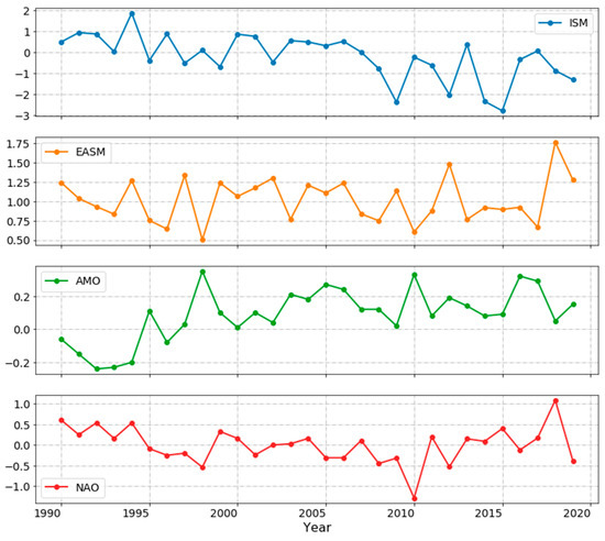
Figure 3.
Large-scale circulations indices over 1990–2019 (ISM: http://apdrc.soest.hawaii.edu/projects/monsoon/seasonal-monidx.html (accessed on 24 September 2021); EASM: http://lijianping.cn/dct/page/1 (accessed on 24 September 2021); AMO: https://psl.noaa.gov/data/correlation/amon.us.data (accessed on 24 September 2021); NAO: https://psl.noaa.gov/data/correlation/nao.data (accessed on 24 September 2021)).
The El Niño/La Niña phenomenon refers to a climatic condition where the surface temperature of the tropical Pacific rises/falls abnormally, causing an uneven distribution of global water vapor that leads to abnormal global climate. In this research, we correlate El Niño/La Niña years proposed by Lei et al. [31] (Table 2) with the years of dramatic changes in lake area in the study area.
Table 2.
El Niño/La Niña years over 1990–2019 [31].
2.3. Methods
2.3.1. Calculate Annual Lake Area
There are two main challenges to obtain annual lake area. First, the specific number and location of lakes are uncertain at the best (if not unknown). Second, local computing resource is insufficient to store and process the large number of images needed. This study used the GEE, a cloud-based geospatial data analysis platform which provides both the imagery and computational resource, for calculating annual lake area.
Due to lake dynamics, a certain lake may consist of several separate waterbodies in some of the years when water level is low. In our study, we treated and combined all the waterbodies that had ever connected during the study period as single lake. For this purpose, we used the “max_extent” band in the JRC data to identify maximally connected waterbodies. Then, we selected only the waterbodies with an area greater than 1 km2 for further processing. Those waterbodies include not only lakes but also rivers connected to them. The border between lakes and rivers is hard to define but we assume that the primary waterbody of a lake is relatively flat and should have a slope close to zero. We used SRTM DEM to calculate the slope for each waterbody pixel. Pixels with a slope greater than 0° are considered rivers and removed from the waterbody. In this step, several patches of waterbody pixels may occur. We visually inspected those patches and only kept the patch that represents the approximate extent of the lake associated with the waterbody. This approach worked effectively for water bodies larger than 50 km2 and the approximate lake extents of 490 lakes were identified this way. The above procedure, however, tends to remove many small waterbodies entirely. So, for waterbodies less than 50 km2, we inspected each waterbody visually and manually drew the lake extents, and we identified 486 more lakes and their extents. Altogether, we identified a total of 976 lakes and their extents in the study area. After removing rivers, each remaining waterbody is treated as the maximum extent of a lake, and its centroid is used as a seed to locate and identify the lake. The maximum lake extent was further extended by a buffer which was used as the lake’s analysis extents to select and clip the Landsat images for reducing the amount of calculation. The buffer distance is determined by the size of the lakes where lakes were roughly divided into five levels with a buffer distance from 1 to 5 km where larger lakes use bigger buffers. The workflow involved in the process is shown in Figure 4.
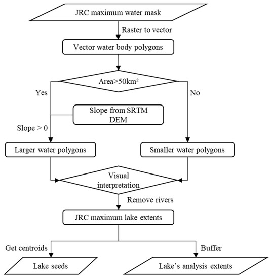
Figure 4.
Workflow for lake identification and generating lake seeds and analysis extents.
All the Landsat images within a calendar year were selected and clipped by a lake’s analysis extent and were then used to generate an annual composite image using the SimpleComposite algorithm in GEE. The algorithm selects the lowest possible range of cloud score at each pixel and then computes per-band percentile values from the accepted pixels. In our study, we set the cloud score range as [0, 10] and the percentile as 0, which means selecting the pixels with cloud scores less than 10 and choosing the lowest value as the pixel value on the composite image for each band. Since water pixels typically have very low value, the annual composite image represents likely the maximum lake area in a year. By using the SimpleComposite function with the chosen parameters, we removed most cloud and generated annual max-water composite images. More details on the function can be found at https://developers.google.com/earth-engine/guides/landsat#simple-composite (accessed on 24 September 2021). Due to sensor difference, we generated an annual composite image using only the images from the same Landsat sensor. For years 1999–2011 and 2013–2019 with images available from two sensors (Landsat 5 and 7 and 7 and 8), two annual composite images were generated and the average area is calculated when both images have good quality.
Normalized Difference Water Index (NDWI) [46,47] was used to extract water pixels on the annual composite images. As waterbodies may have different spectral characteristics in time and space on the composite images, adaptive NDWI thresholds were used to segment water pixels. In this study, the OTSU algorithm [48,49,50] was used to determine an adaptive threshold (see Section 4.3 in Discussion) using the pixels within a certain buffer along a lake’s shoreline which was detected using the Canny edge detector algorithm available in GEE. The Canny edge detector algorithm first removes high-frequency noise using Gaussian filtering, then calculates the gradient based on the NDWI value, and finally obtains the land-water edge by setting a threshold. In our research, the sigma value of the Gaussian filter is set as 1.5, and the gradient threshold is set as 0.4. The determination on those parameters is further discussed in Section 4.2. For lakes with noisy composite images, we use the Quality Assessment Band (QAB) in Landsat to remove noises such as sensor saturation, cloud shadows and terrain shadows before creating annual composite images.
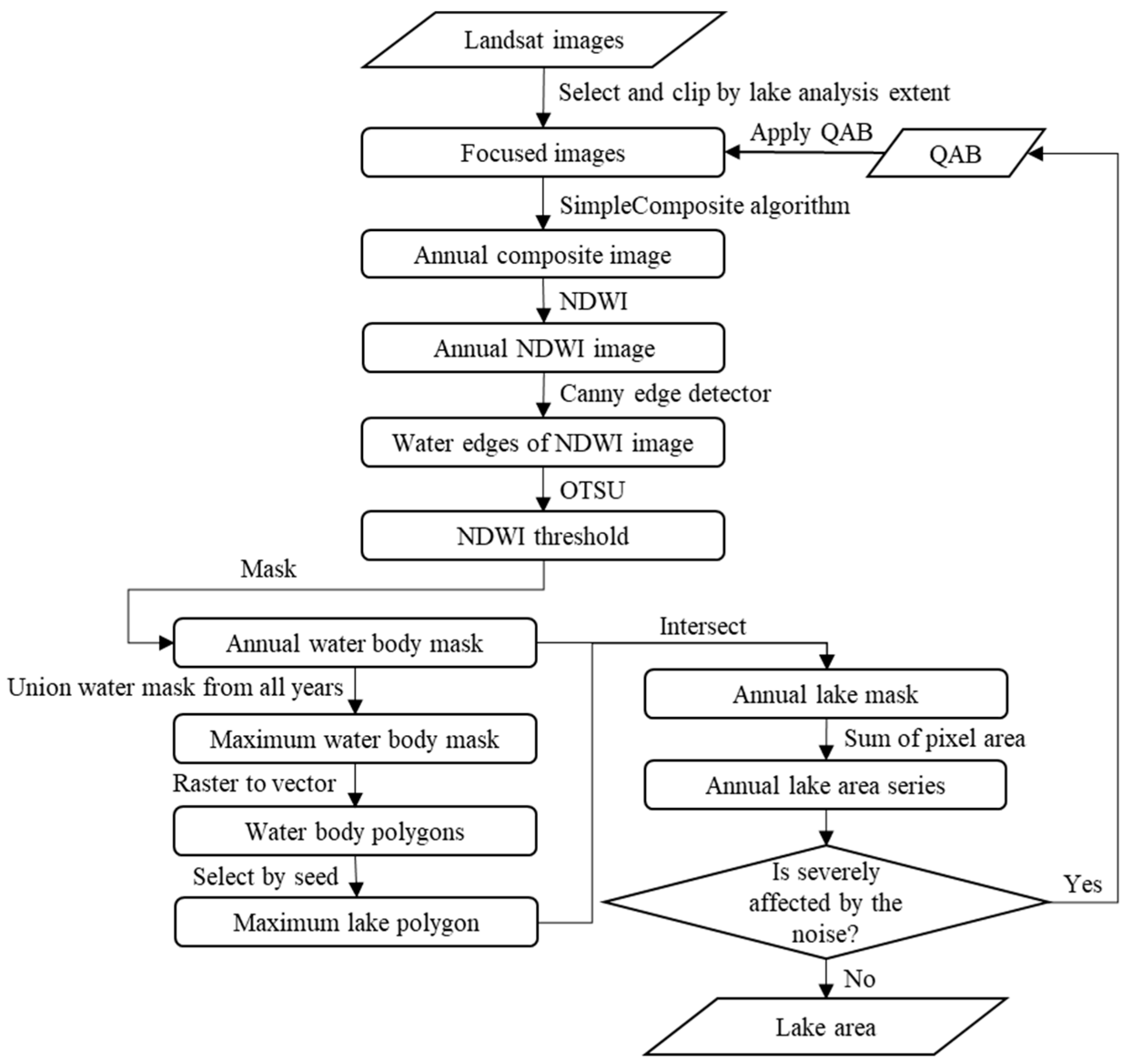
One challenge in calculating annual lake area is that a lake may have several separate waterbodies in some of the years. For this purpose, we union the water masks of all the years within a lake’s analysis extent and from which, we then identified the spatially connected water mask which contains the lake seed as the maximum lake extent polygon for the years. The polygon is then used to identify all the lake pixels from annual water masks. In this way, even if a lake has separate waterbodies in some years, all the waterbodies are considered as parts of the same lake. The area calculation process is shown in Figure 5.
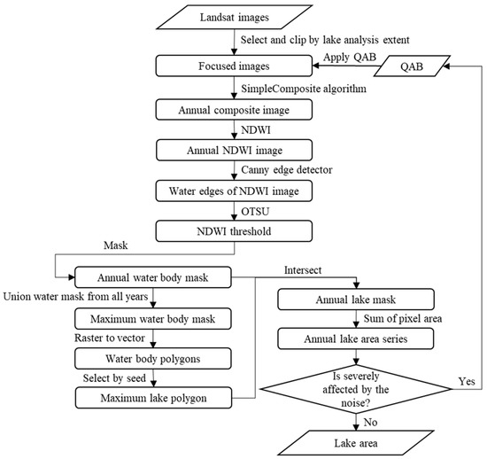
Figure 5.
Workflow for lake area calculation.
We checked the area automatically calculated using the workflow shown in Figure 5. If the area in a certain year is very different from the years before and after it or if the areas from different sensors in the same year are quite different, we manually examined the composite images. If none of the annual composite images have good quality and the waterbodies could not be extracted correctly from them, lake area for the year will be marked as no data. For the years with missing data, we estimated lake area using linear interpolation (see Section 4.1 in Discussion). In total, we calculated the annual area of 976 lakes whose largest area during 1990–2019 is greater than 1 km2.
2.3.2. Lake Area and Climate Relationship
Linear regression and Mann–Kendall test were used to analyze lake area change trends [51]. We also examined possible relationships between lake area and local climatic variables (temperature and precipitation) and large-scale circulation indices by calculating their correlation coefficients. For the correlation analysis, Pearson correlation coefficient (r) was used, and all the statistical significance level (P) for correlation coefficients was evaluated at 0.05 unless otherwise stated. Previous research found El Niño/La Niña events may cause abnormal drought (rainfall) in parts of the TP [31], which may lead to change in lake area. We used extreme value analysis to examine whether there is a sudden area decrease (increase) in the El Niño/La Niña years based on a de-trended lake area series. The detrending was conducted by subtracting linear trends from the original lake area series data (i.e., the difference detrending method) to avoid the difficulty of finding the extreme points due to potential trends in the original area.
3. Results
3.1. Lake Area Validation
We used two existing data sources to verify our lake area. The first dataset is from Zhang et al. [18] which contains 12 years (1970s, 1990, 1995, 2000, 2005, 2010 and 2013–2018) of lake area in the TP and has been used in several studies [18,33]. The other dataset is the lake water level/area/storage dataset provided by the LEGOS Hydroweb [52], which contains the area of some large lakes in the EBTP.
In Zhang’s data, lake areas in 1990, 2000 and 2010 were visually interpreted and manually digitized and are better reference data, and areas in other years were obtained through automatic image analyses similar to our method. We used symmetric absolute percentage error (sAPE) [53] to evaluate our data, which can be calculated as follows:
where t is a year, is our lake area in year t, is the validation lake area in year t. The sAPE ranges in [0, 2], and the smaller the value the smaller the difference between the datasets.
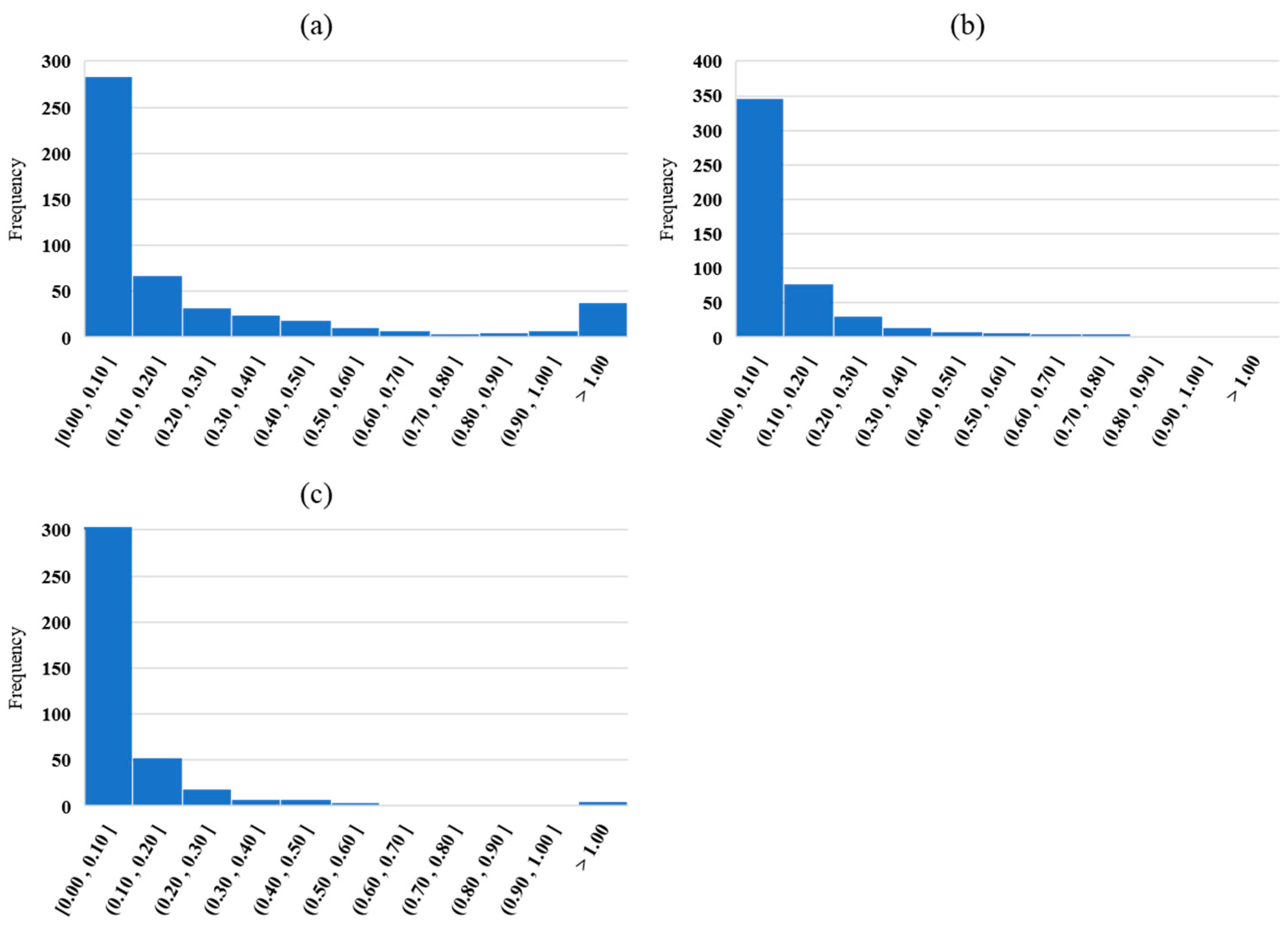
We used 492 lakes which are common both in our and Zhang’s data to calculate the sAPEs in 1990, 2000 and 2010. As we can see in Figure 6, the sAPEs are mainly in [0, 0.1] in the three years. In 1990, 2000 and 2010, there are 282 (57%), 346 (70%), and 398 (81%) lakes whose sAPEs are less than 0.1, respectively, and there are 349 (71%), 423 (86%), and 450 (91%) lakes whose sAPEs are less than 0.2. Overall, for most lakes, our lake area is consistent with Zhang’s lake area. Table 3 shows some statistics on the sAPEs. From 1990 to 2010, the mean and standard deviation of the sAPEs keep decreasing as the number of available Landsat images continues to increase, which produces better annual composite images. Our lake area is calculated based on annual composite images while Zhang’s lake area is calculated using the best image within a 3-year window for the year of 1990 and 2000. For 2010, Zhang’s lake area is calculated using the best images in October of the year, which has the smallest mean and standard deviation in sAPE when compared with our data.

Figure 6.
Histograms of the sAPEs for 492 lakes in 1990 (a), 2000 (b) and 2010 (c).
Table 3.
sAPE statistics in 1990, 2000 and 2010.
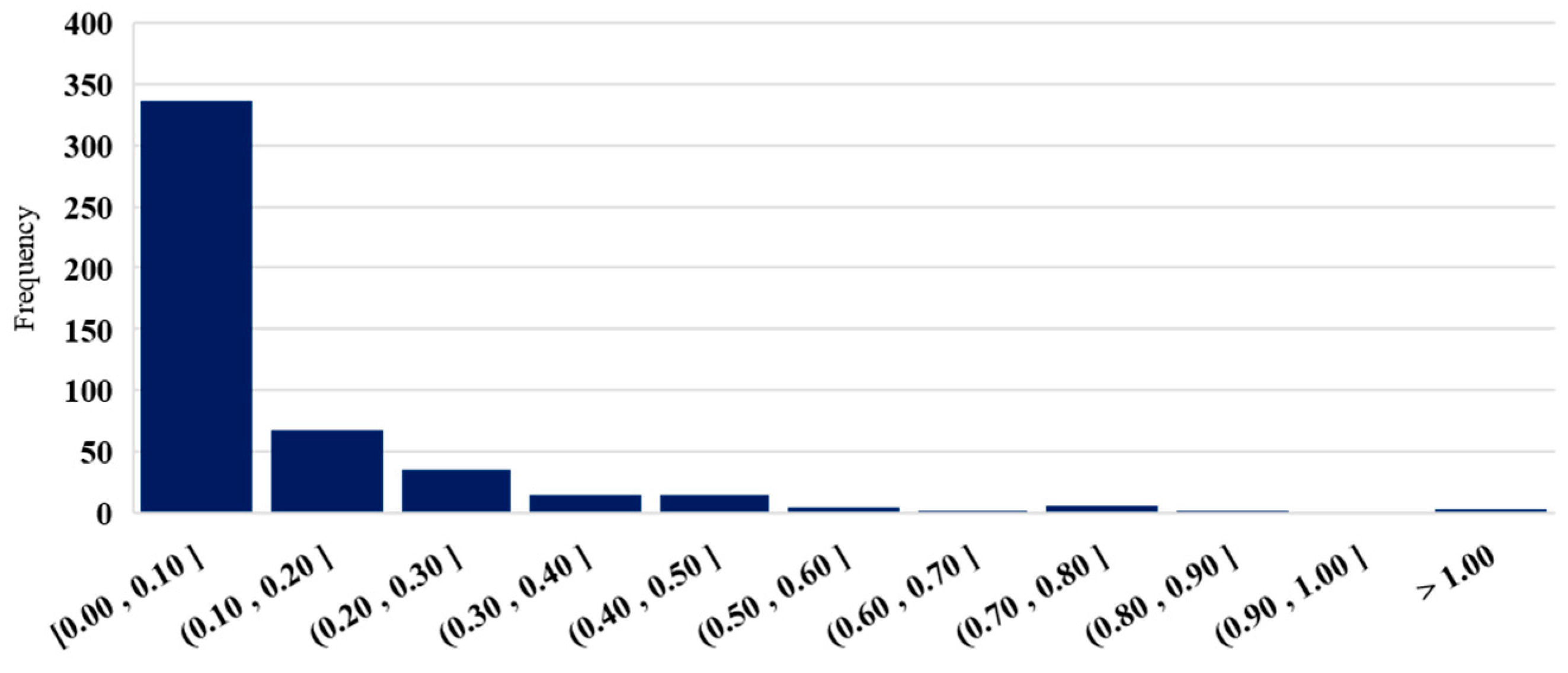
We further calculated the average sAPE for 492 lakes in 11 years (1990, 1995, 2000, 2005, 2010 and 2013–2018) using our and Zhang’s lake area data and the histogram, as shown in Figure 7. There are 337 lakes (68%) with an average sAPE less than 0.1 and 405 lakes (82%) with an average sAPE less than 0.2, which show, for most lakes, our lake area is consistent with Zhang’s data.

Figure 7.
Histogram of 11-year average sAPE for 492 lakes.
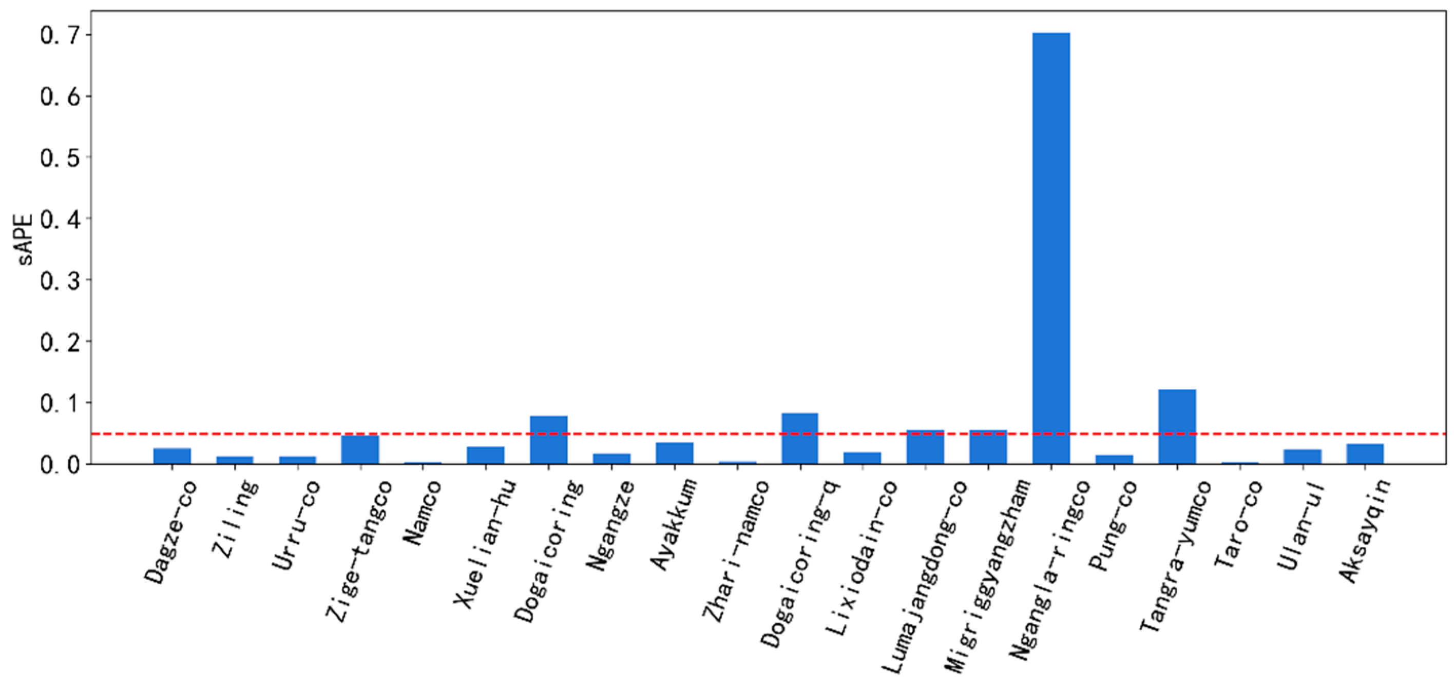
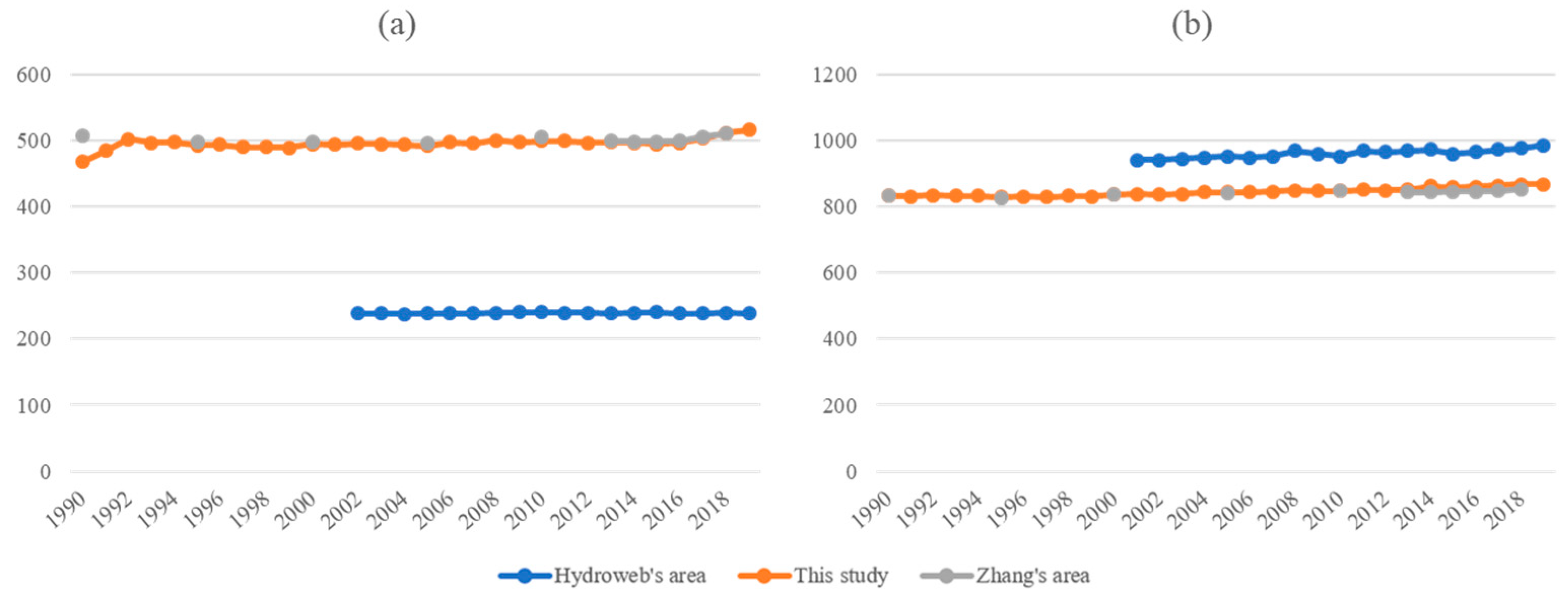
We also compared the area series of 20 lakes from LEGOS Hydroweb with our data. Those 20 lakes are large lakes in the study area and their total area in 2019 accounts for 35.5% of the total area of the 976 lakes. The length of the Hydroweb area series varies between 9 and 27 years. The average sAPEs of those 20 lakes are shown in Figure 8, where 80% the lakes have their sAPE values less than or close to 0.05. Only lake Ngangla-ringco and Tangra-yumco have a value over than 0.1, and Ngangla-ringco has the worst average sAPE of 0.7.

Figure 8.
The average sAPEs for 20 overlapping lakes comparing our results with Hydroweb data.
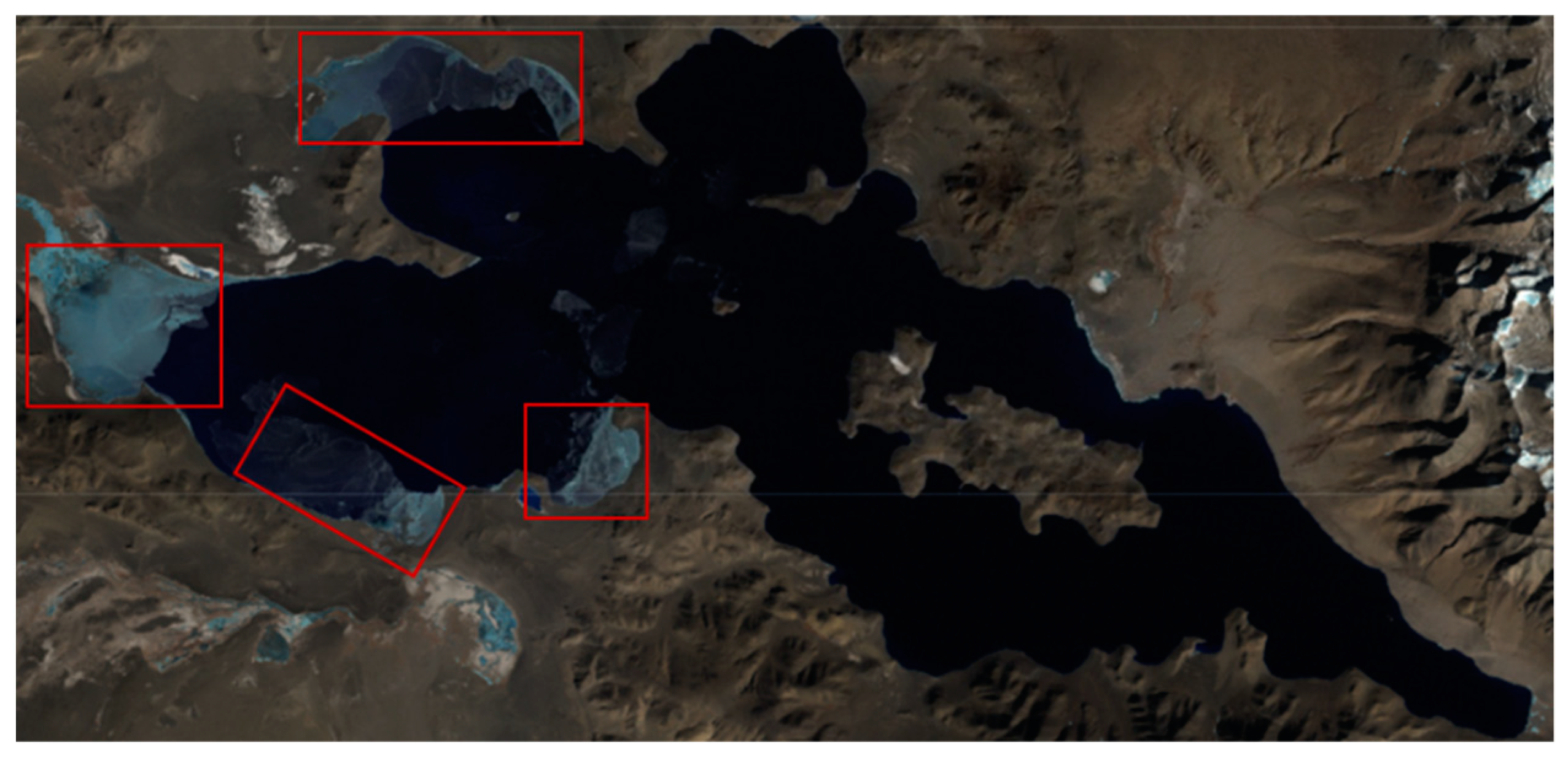
Figure 9 compares our area with Zhang’s and Hydroweb’s area for the two lakes. Our data maintains a high consistency with Zhang’s data with low average sAPEs (0.013 and 0.010) and both our and Zhang’s data have a large difference from Hydroweb’s data. For lake Ngangla-ringco, our area in 1990 has a relatively large difference from Zhang’s area. By checking the composite image, we found the lake is partially covered by ice (Figure 10) and the lake could not be completely extracted. So, lake area for 1990 was interpolated using the area in 1991 and 1992 but it still has relatively a large difference with Zhang’s data.
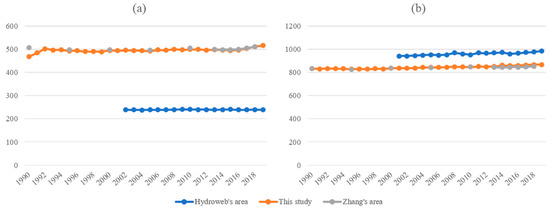
Figure 9.
Comparison of lake area series for lake Ngangla-ringco (a) and Tangra-yumco (b).

Figure 10.
Composite image for lake Ngangla-ringco in 1990 using Landsat 5 images. Red boxes indicate frozen lake water which was not correctly identified as lake in our data.
3.2. Change of Lake Area
The total area of the 976 lakes shows an upward trend during the period of 1990–2019 (Figure 11). In 1990, total lake area is 26,126.86 km2, and in 2019 it became 37,355.68 km2, with an increase of 11,229 km2 or 42.99%. Total lake area has been increasing in most of the years except for 1991–1995, 1996–1997, and 2012–2015. Based on Mann–Kendall trend analysis, total lake area showed a significant increase trend of 432.52 km2 per year. Bian et al. [54] also indicate over 13% lake area increase between the first (1999–2001) and second (2009–2011) National Inventory of Wetland Resources in Qinghai Province and Tibet Autonomous Region. We also performed Mann–Kendall trend analysis for each sub-region. The slope (increase rate) and coefficient of determination (Tau) are shown in Table 4. While the Tau values for R01 and R08 are below 0.6, they are all significant at the significance level of 0.001.
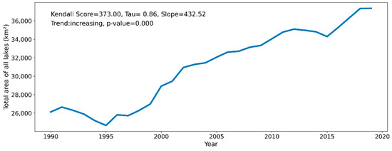
Figure 11.
Change in total lake area in the EBTP over 1990–2019 with the results from Mann–Kendall trend analysis.
Table 4.
Mann–Kendall analysis on total lake area in each sub-region (Tau values marked with * indicate significance at the level of 0.001, increasing rate = slope/average lake area).
We performed Pettitt mutation point detection analysis [55] for each lake. The analysis is a non-parametric method for identifying the mutation point in a time series and is commonly used in hydrological change studies [56]. In the method, Pettitt proposed that when the p value is less than 0.5, the mutation point is considered significant [55]. We found that 947 lakes (97%) and 862 lakes (88%) have significant mutation points at the 0.5 and 0.05 significance level, respectively. At the 0.05 level, 290 lakes (29.7%) experienced a trend change in 2005, and 468 lakes (48%) experienced a trend change between 2003 and 2006. The mutation year for total lake area is also 2005 at the significance level of 0.05. As such, we further examined lake area change over 1990–2005 and 2005–2019, in addition to 1990–2019.
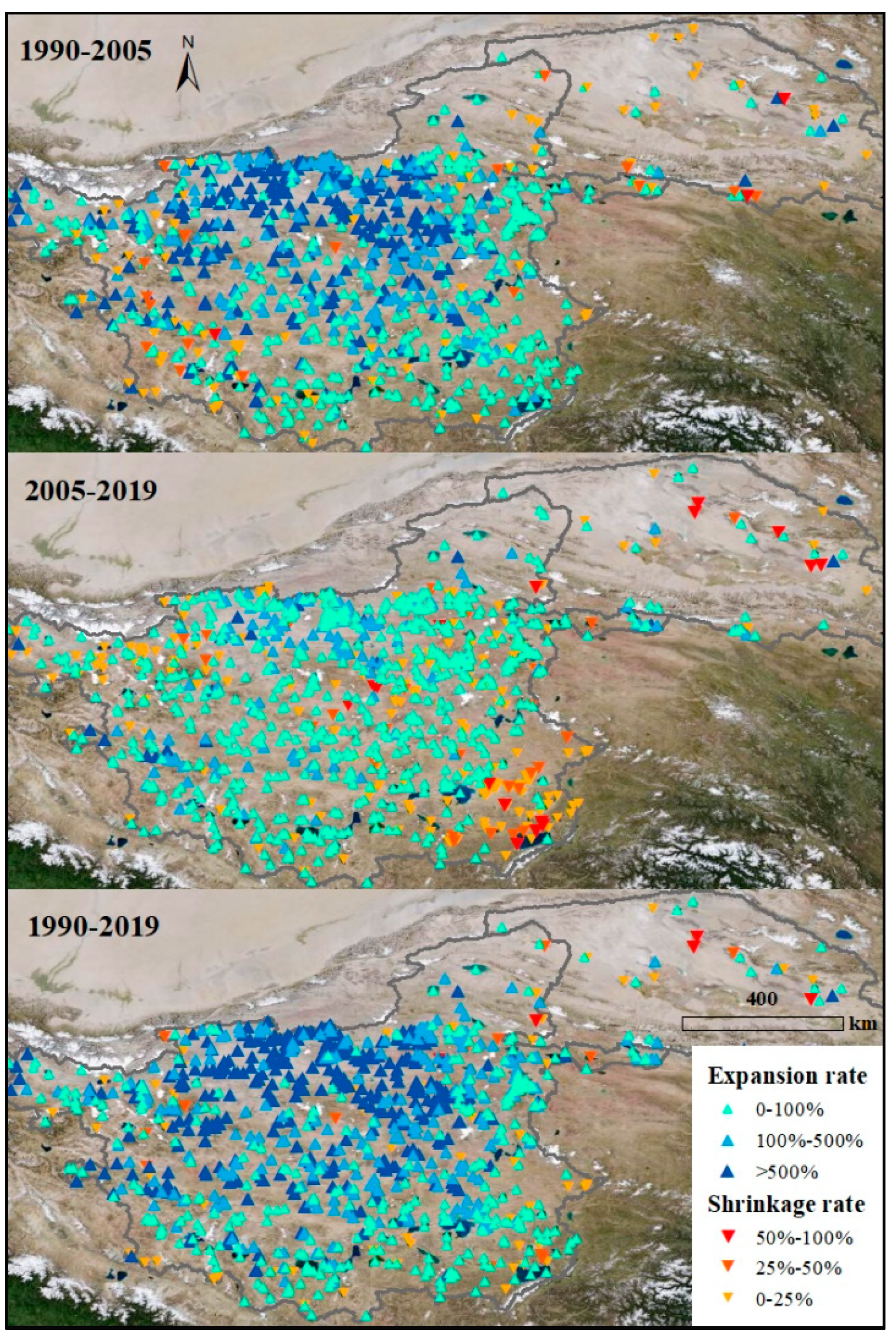
Figure 12 shows lake area trends in the three time periods. From 1990 to 2005, 874 lakes (89.5%) experienced area expansion, of which 463 lakes (47.4%) expanded by more than 100%, and 263 lakes (26.9%) expanded by more than 500%. These lakes are mainly located in the north-center part of the IB. Meanwhile, only 102 lakes (10.5%) experienced area shrinkage, and these lakes are largely in the QB and also scattered around the western edge of the IB. The overall expansion rate during this period is 451.26 km2·year−1. From 2005 to 2019, 758 lakes (77.7%) experienced area expansion, though most rates were less than 100%. Two hundred and eighteen lakes (22.3%) experienced area shrinkage, of which 44 lakes are located in the southeast corner of the IB. The overall expansion rate during this period is 345.63 km2·year−1, which is 76.6% of the expansion rate in 1990–2005. For the entire period of 1990 to 2019, 894 lakes (91.6%) experienced area expansion, and the expansion rates of 548 lakes (56.1%) exceeded 100% and 313 lakes (32.1%) exceeded 500%, most of which are located in the north-central part of the IB. Only 82 lakes (8.4%) experienced area shrinkage, which are scattered throughout the study area. The overall expansion rate during this period is 451.19 km2·year−1 (Figure 11). Overall, lakes with expanded area are far more than the lakes with reduced area, and the rate of expansion (46.93%) is also much higher than that of shrinkage (12.82%).
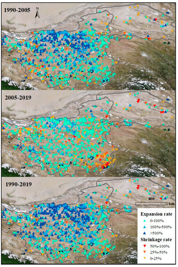
Figure 12.
The rates of area change for 976 lakes in the study area during three time periods: 1990–2005, 2005–2019 and 1990–2019.
3.3. Lake Area and Local Climate
In the EBTP, although it is hard to tell the correlation between annual mean temperature or annual precipitation with total lake area (Figure 13), annual precipitation has a higher correlation coefficient (r = 0.67, p < 0.05) than annual mean temperature does (r = 0.45, p < 0.05). Total lake area shows a strong correlation (r = 0.66, p < 0.01) with annual precipitation but not with annual mean temperature (r = 0.28, p = 0.15) in the IB, and it shows a moderate correlation with both annual mean temperature (r = 0.48, p < 0.05) and annual precipitation (r = 0.49, p < 0.05) in the QB.
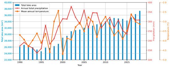
Figure 13.
Total lake area, annual mean temperature, and annual precipitation in the EBTP over 1990–2019.
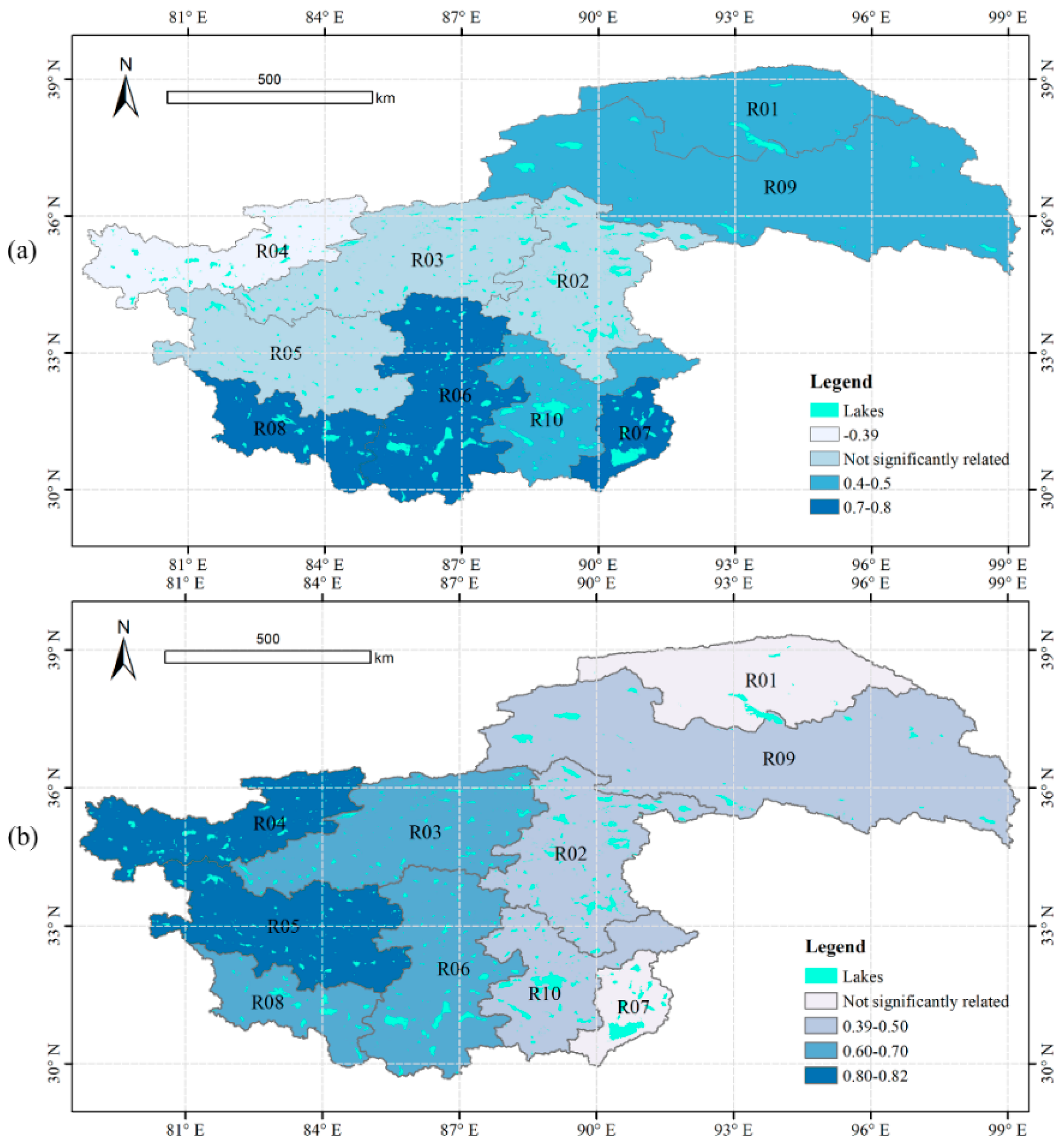
We further explored the relationships in each sub-region. Figure 14a shows the spatial difference in sub-regional correlation between lake area and annual mean temperature. Central and southern sub-regions in the IB show significant correlation with annual mean temperature (r > 0.4, p < 0.05), and sub-regions R06, R07 and R08 have the highest correlation (r > 0.7, p < 0.05). Lake area shows a weak correlation (0.4 < r < 0.5, p < 0.05) with annual mean temperature in the two sub-regions in the QB. The correlation between lake area and annual precipitation is shown in Figure 14b. Most sub-regions, except for R01 and R07, show a significant correlation (r > 0.39, p < 0.05), where the highest correlation is in the western sub-regions of the IB (r = 0.8, p < 0.05) and the correlation gradually decreases from west to east. Overall, there is a significant correlation between lake area and annual mean temperature and annual precipitation in the EBTP.

Figure 14.
Correlation coefficient (r) between lake area and annual mean temperature (a) and annual precipitation (b) at sub-regional scale.
3.4. Lake Area and Large-Scale Atmospheric Circulations
3.4.1. Impact of Regional Monsoon Systems
Previous studies [16,26,27,28,29] have shown that monsoon systems (EASM and ISM) can transport water vapor to the TP and form precipitation. On the other hand, due to high altitude and the blockage of high mountains, monsoon’s influence might be limited. We explored the correlation between lake area and regional monsoon systems at three different scales: the entire EBTP, two large watersheds (IB and QB), and sub-regions. We found there is no significant correlation (r < 0.3, p > 0.1) between total lake area and the EASM at any scale. This is consistent with Chang et al. [28] who studied monsoon impacts on the precipitation in China and concluded that the EASM does not affect precipitation in the TP at intra-annual and inter-annual time scales.
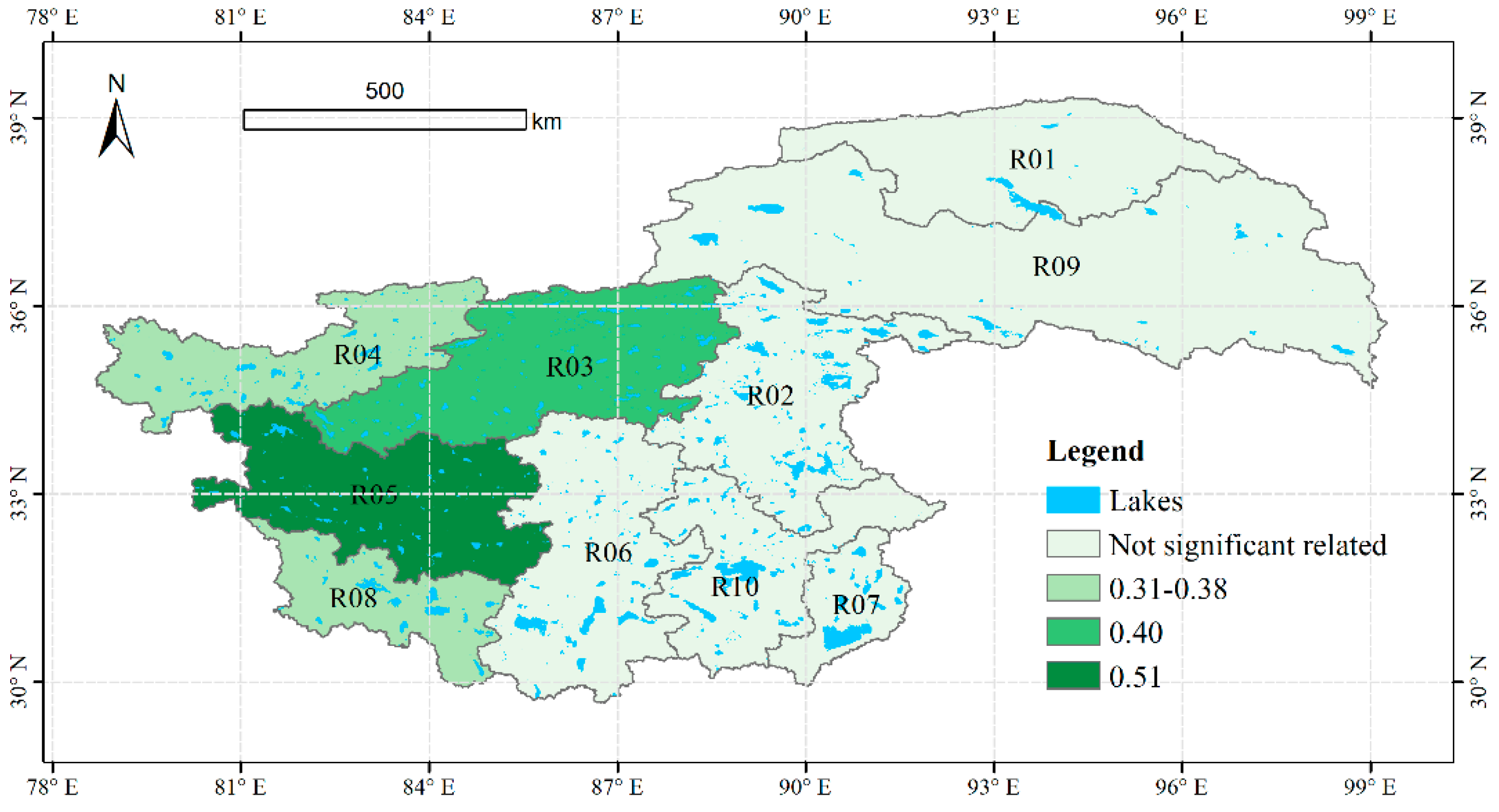
For the relationship between ISM and lake area, we found that while lake area shows an overall upward trend, and ISM has been weakening in the past 30 years [57]. In most sub-regions, lake area has a significant negative correlation with ISM index. Considering that the ISM brings water vapor to the TP, which should promote lake area expansion, we detrended the ISM index and lake area series and then calculated the correlation. In this case, there is no significant correlation (r < 0.3, p > 0.1) between lake area and ISM index at the scales of entire EBTP and two large watersheds. However, ISM index has a significant correlation (r = 0.41, p < 0.05) with precipitation in the IB. At sub-regional scale, ISM index has some correlation (r > 0.31, p < 0.1) with lake area in western sub-regions (R03, R04, R05 and R08) of IB (Figure 15), but has no significant correlation with lake area in eastern sub-regions. Lake area in the western sub-regions is also highly correlated with local precipitation (r > 0.60, see Figure 14b) and the ISM index has a significant correlation (p < 0.05) with the precipitation in R03 (r = 0.39), R05 (r = 0.57) and R08 (r = 0.60). According to previous studies [26,27,28], ISM index is related to precipitation in western IB. Therefore, the high correlation between ISM index and lake area (as well as precipitation) may indicate that ISM likely impact lake area by affecting local precipitation, especially in the western IB.

Figure 15.
Correlation coefficient (r) between lake area and the ISM index at sub-regional scale.
3.4.2. Impact of Atmospheric Circulation
The AMO and NAO are atmospheric circulation indices related to westerlies, and they are likely related to the climate in the TP remotely. So, we explored the connection between the two global atmospheric circulations and lake area at three spatial scales: the entire EBTP, two large watersheds and sub-regions. As shown in Table 5, AMO shows significant correlation (p < 0.05) with lake area (r = 0.56), precipitation (r = 0.58) and temperature (r = 0.56) in the EBTP. It also shows significant correlation in the two large watersheds (IB and QB). Sun et al. [58] found that AMO has been in a positive phase since the mid-1990s (see Figure 3), which has led to both a northward shift and weakening of the subtropical westerlies jet stream at 200 hPa near the TP through a series cyclonic and anticyclonic anomalies over Eurasia. By weakening the westerlies and strengthening the southwest wind on southern IB, those cyclones and anticyclones jointly promoted the convergence of water vapor over the IB and caused more water vapor transported into IB from the Arabian Sea (the dominated region of west ISM, see Figure 1). Accordingly, summer precipitation over inner TP has increased [58], which may explain the connection between lake area change and AMO to some extent.
Table 5.
Correlation coefficients between global atmospheric circulation indices and lake area, temperature and precipitation for the entire EBTP and in the IB and QB. Values marked with * represent significant correlation at the 0.05 level and bold values represent significant correlation at the 0.1 level.
From the perspective of water vapor transport, north of 35° latitude in the TP is mainly controlled by westerlies [30] and the NAO index reflects the strength of the westerlies. The QB is located in the westerly domain and previous study has shown that glacier area variation in central TP is positively associated with NAO [25]. However, our study found no significant correlation between lake area and the NAO index. At the significance level of 0.1, there is a negative correlation (r = −0.35) between NAO index and precipitation in the QB. Correlation analysis results in the sub-regions are similar to those in the IB and QB. Based on the above analyses, it is still unclear whether there is connection between NAO and lake area change in the EBTP.
3.4.3. Lake Area and the El Niño/La Niña Events
Previous studies [31] show that El Niño/La Niña events can cause abnormal drought (rainfall) in parts of the TP. By examining the years in which lake area decreased (increased) significantly and comparing them with El Niño/La Niña years, we can explore the connection between lake area and El Niño/La Niña events in the EBTP. To eliminate the impact of the general upward trend in lake area, we first detrend the lake area, and then identify the years of lake area valley (peak). We define the valley (peak) year as the year if its lake area is smaller (larger) than the area of years before and after it. We then match the valley (peak) years with the years of El Niño/La Niña events. We explored the connection between the El Niño/La Niña events and lake area at four different scales: the entire EBTP, two large watersheds, sub-regions and individual lakes.
There are three lake area valley years that match the El Niño years of 1997, 2009 and 2015 in the EBTP. Among them, 1997 and 2015 are two strong El Niño years and they match the lake area valley years in the IB. There are no matched valley years in the QB (Table 6), which may indicate that the El Niño events mainly affect the lake area in the IB. For La Niña events, there is one lake area peak year that matches the La Niña year of 2008 for the IB, 1999 for the QB and 2011 for the EBTP.
Table 6.
Years with matching El Niño/La Niña events and lake area valley (peak) in the EBTP, IB and QB.
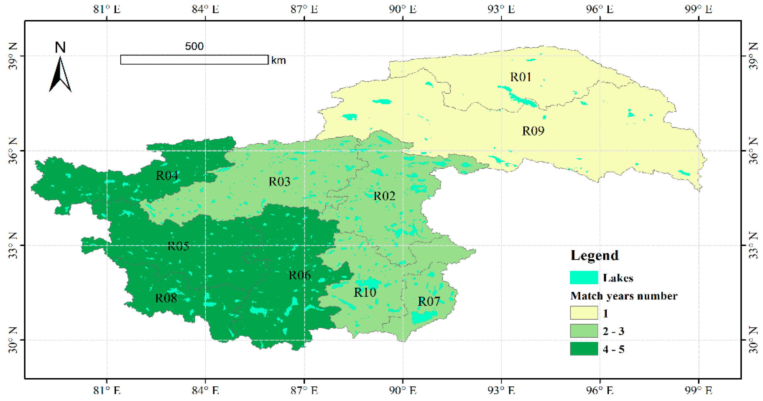
At the sub-region scale, while the number of matched years is low for the sub-regions in the QB, there are more matched years in the sub-regions in the IB, especially in R04, R05, R06 and R08 (Figure 16) where lake area is also highly correlated with precipitation, indicating that the El Niño/La Niña events may be connected with lake area by affecting local precipitation. Previous studies have also shown that lake area change in the central TP is greatly affected by the El Niño/La Niña events [31,59].

Figure 16.
Number of matching matched years between El Niño/La Niña years and lake area valley (peak) years at sub-regional scale. There is a total of 11 El Niño and La Niña years over 1990–2019 (see Section 2.2).
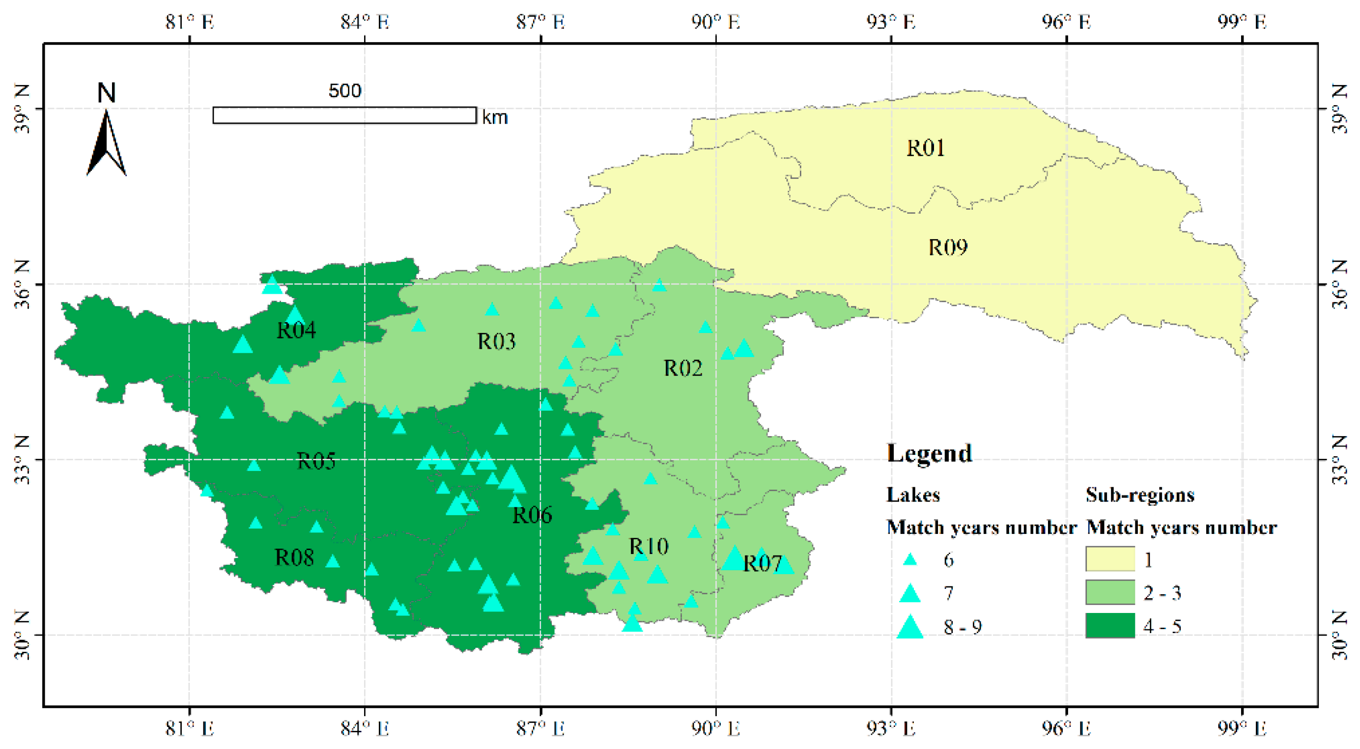
Lei et al. [31] explored the impact of El Niño/La Niña events on individual lakes, and found some lakes are very sensitive to El Niño/La Niña events. We also examined the connection between El Niño/La Niña events and individual lake area. We first detrend the area series of the 976 lakes, identify the valley (peak) years, and then find the matching valley (peak) years with El Niño/La Niña years for each lake. There is a total of 11 El Niño and La Niña years over 1990–2019. Lakes with the number of matching years greater than or equal to 6 years is shown in Figure 17. It can be seen that lakes with high matching years are located in the IB, which is consistent with the observation at the sub-region scale.
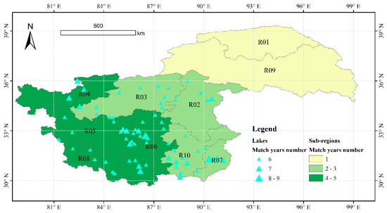
Figure 17.
Lakes with the number of matching years greater than or equal to 6 years.
4. Discussion
4.1. Noise on Composite Images
We composed annual images using all the images available in a year with a cloud score less than 10. However, due to clouds, cloud shadows, and sensor failure (such as Landsat 7 stripes), it still may have noises on the lakes in some annual composite images and complete lake area may not be extracted from these images. We manually checked those images and interpolated their area (see Section 2.3.1). As shown in Figure 18a, the percentage of lakes with erroneous data varies from year to year. For the years in 1999–2011 (Landsat 5 and 7) and 2013–2019 (Landsat 7 and 8), there are two annual composite images from two sensors and the proportion of noisy images is relatively low, with an average of 1.20%. For other years, the proportion is relatively high, with an average of 6.35%. For different Landsat sensors, the proportion is about 10%, 7%, 4% for Landsat5 (1990–2011), Landsat7 (1999–2019), Landsat8 (2013–2019), respectively (Figure 18b). Proportions of noisy annual composite images in different sub-regions are shown in Figure 18c. R07 has the lowest proportion of 1.17%. R04, R05 and R08, which are located in the western edge of the study area, have relatively high proportions that exceed 4%. The remaining sub-regions have a proportion that ranges from 2.2% to 3.1%. Lake area for those noisy years was estimated using linear interpolation.
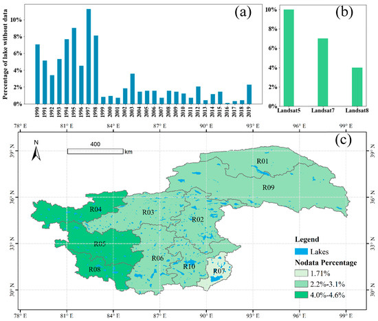
Figure 18.
Proportions of noisy annual composite images. (a) The proportion of lakes with noisy data in 1990–2019; (b) The proportion of noisy data for different sensors; (c) The proportion of noise data in the sub-regions.
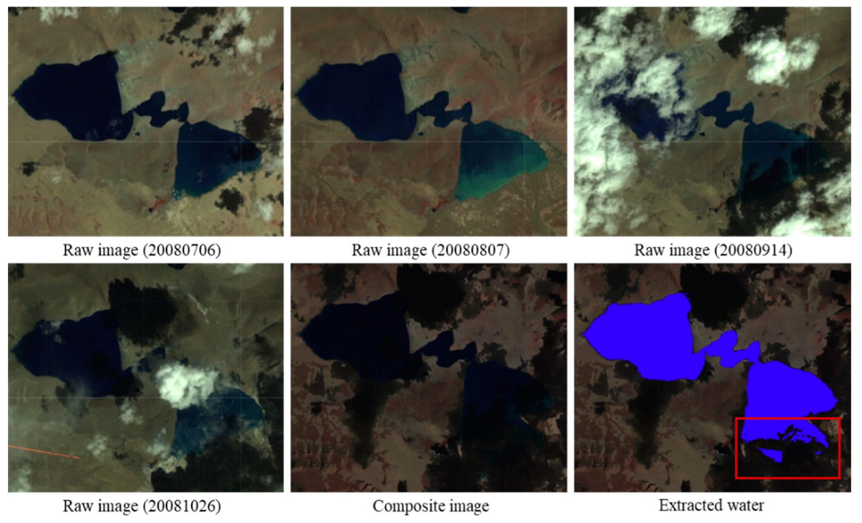
In addition to unusable annual composite images, the SimpleComposite algorithm used in this study also exacerbated the impact of shadows for some lakes. Our method tries to identify the maximum water extent from the composite images by picking the lowest value among the pixels with a cloud score less than 10. This approach will pick up the shadows on composite images as they also have very low pixel values. We found there are cases where the shadows are connected to lakes, our method may identify the shadows as lake and overestimate lake area as shown in Figure 19 (not all the raw images used in the composite image are shown).

Figure 19.
Raw images, composite image and extracted lake extent for lake Nading Co in 2008 using Landsat5 imagery. Lake water in the red box cannot be extracted correctly due to cloud shadow contamination.
4.2. Canny Edge Detector Parameters
In our method, several parameters were used to identify lakes and calculate their area. Those parameters, such as the cloud score range and pixel value percentile in the SimpleComposite algorithm, the gradient threshold and size of the Gaussian filter in the Canny edge detection algorithm, and the buffer size for clipping composite images, can affect the results to various extents. We conducted numerous tests and used the parameter values that produced good results for most lakes.
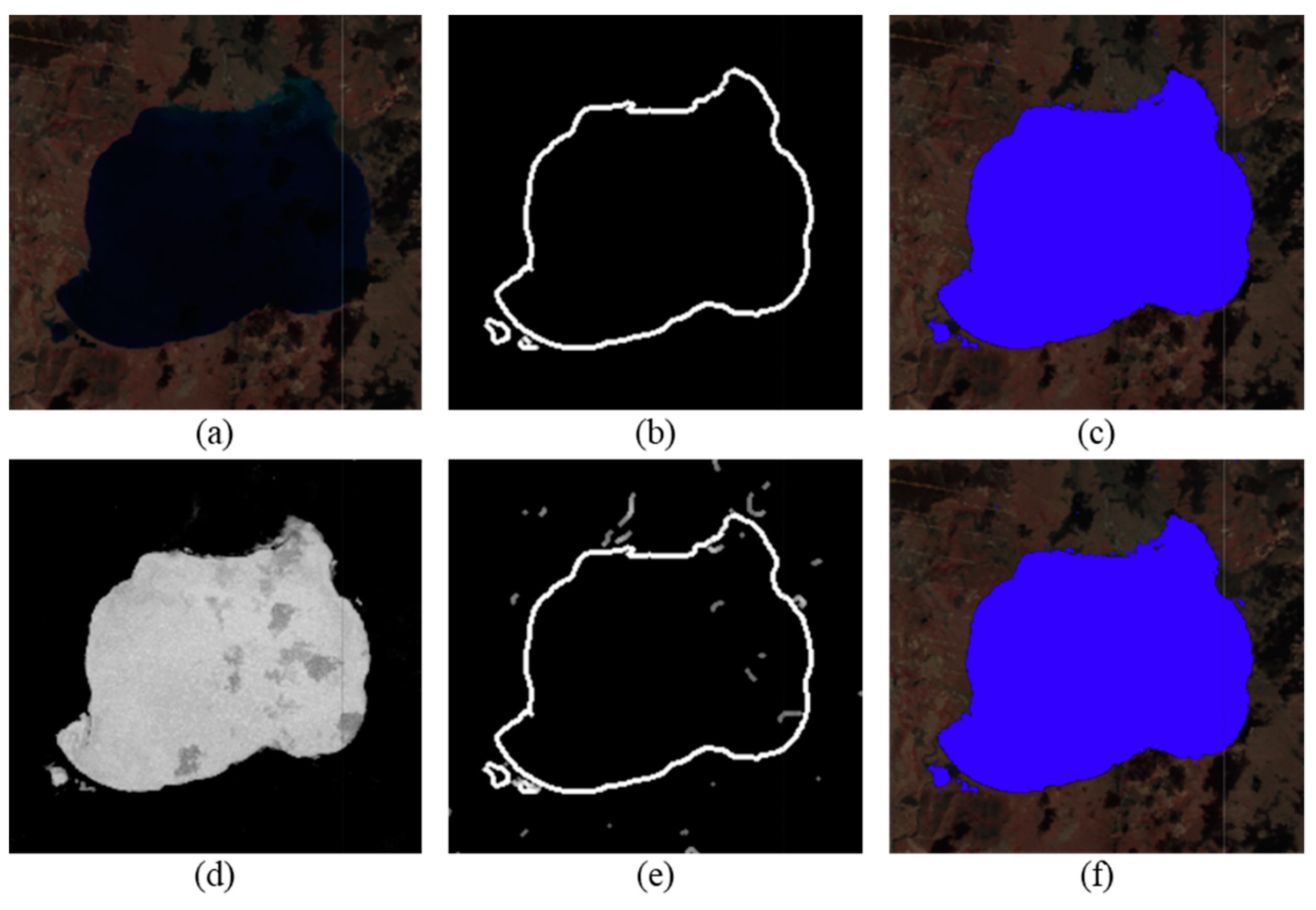
Taking the parameters in the Canny edge detector as an example, different parameter settings can detect different edges which may lead to different NDWI thresholds as it may detect not only lake edges but also cloud shadow, Landsat7 strips and other edges on a composite image. The parameter settings may vary with lakes, years, sensors to detect more accurate water-land edges. We tried and manually examined many parameter settings and found the parameter settings (hereafter standard parameters) with a gradient threshold of 0.4 and Gaussian filter sigma value of 1.5 worked the best for most of the lakes in the study area. In most cases, the NDWI thresholds obtained with the standard parameters are reasonable. As an example, lake area (Figure 20c) obtained using a better ad hoc parameters manually identified is 72.879 km2 and the lake area (Figure 20f) obtained using the standard parameters is 72.931 km2 with a difference of only 0.0007%. There are, however, some NDWI images that the detected edges may be erroneous using the standard parameters. In this case, we discarded the composite images and calculated their area by interpolation.

Figure 20.
Edges and water bodieswaterbodies identified using ad hoc parameter settings manually identified and the standard parameter settings. (a) composite image; (b) edges detected using the ad hoc parameters; (c) lake identified using the ad hoc parameters; (d) NDWI image calculated from the composite image; (e) edges detected using the standard parameters; (f) lake identified using the standard parameters.
4.3. NDWI Thresholds
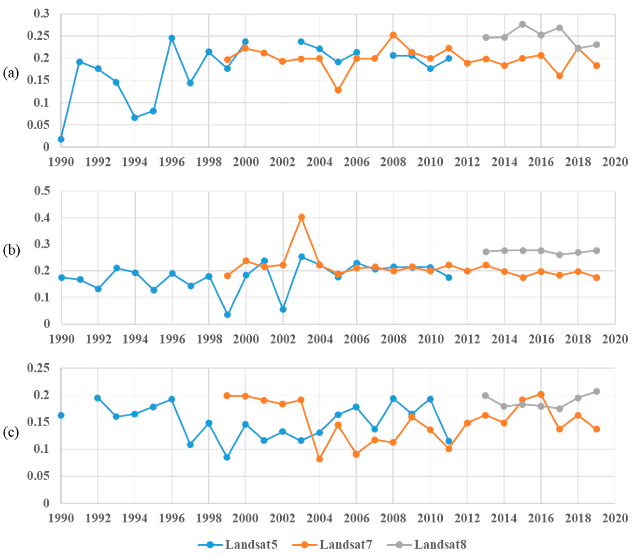
In this study, we used adaptive NDWI threshold to segment lake pixels as water characteristics on the composite images may vary with different lakes, Landsat sensors and years. Figure 21 shows the NDWI thresholds for Ganju Lake (~10 km2), Dagze-co (~200 km2) and Tangra-yumco (~800 km2) from 1990 to 2019. Each lake has a different threshold range in those years. With the same Landsat sensor, the threshold varies through the years, and for the same year, different Landsat sensors have different thresholds. Fom 2013 to 2019, Landsat 8 composite images have higher thresholds than those from Landsat7. Those examples show that it is necessary to use adaptive thresholds for different lakes, Landsat sensors and years.
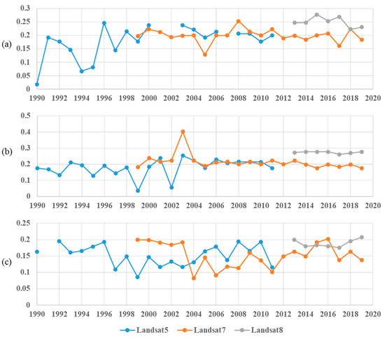
Figure 21.
NDWI thresholds in different years with different Landsat sensors for lake Ganju Lake (a), Dagze-co (b) and Tangra-yumco (c).
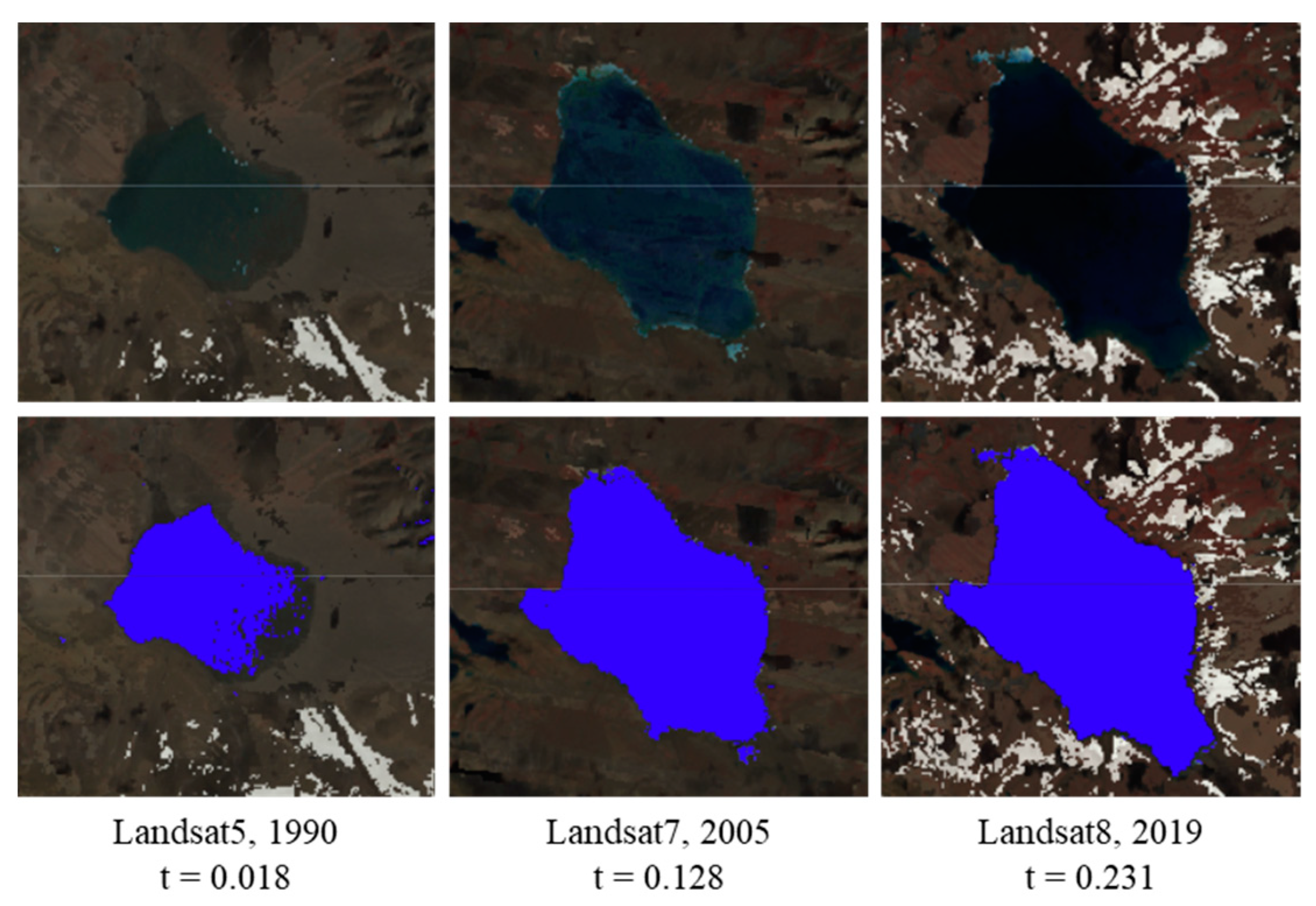
For lakes that were initially small but expanded rapidly in later years, it is especially necessary to use an adaptive NDWI threshold as lake water characteristics may change significantly over the years. As the example shown in Figure 22, lake Ganju was shallow and muddy in the early years. Later, as the lake expanded and its water became deeper and darker. As majority of the lakes in the study area experienced significant expansion, using adaptive NDWI threshold provided more accurate lake identification and area calculation.
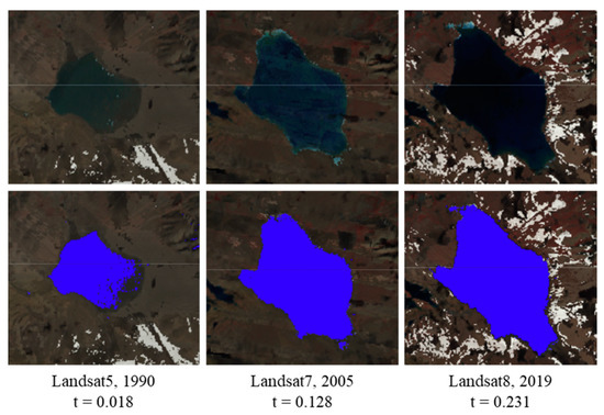
Figure 22.
Composite images, detected water extents and NDWI thresholds for lake Ganju Lake in different years (t is the NDWI threshold).
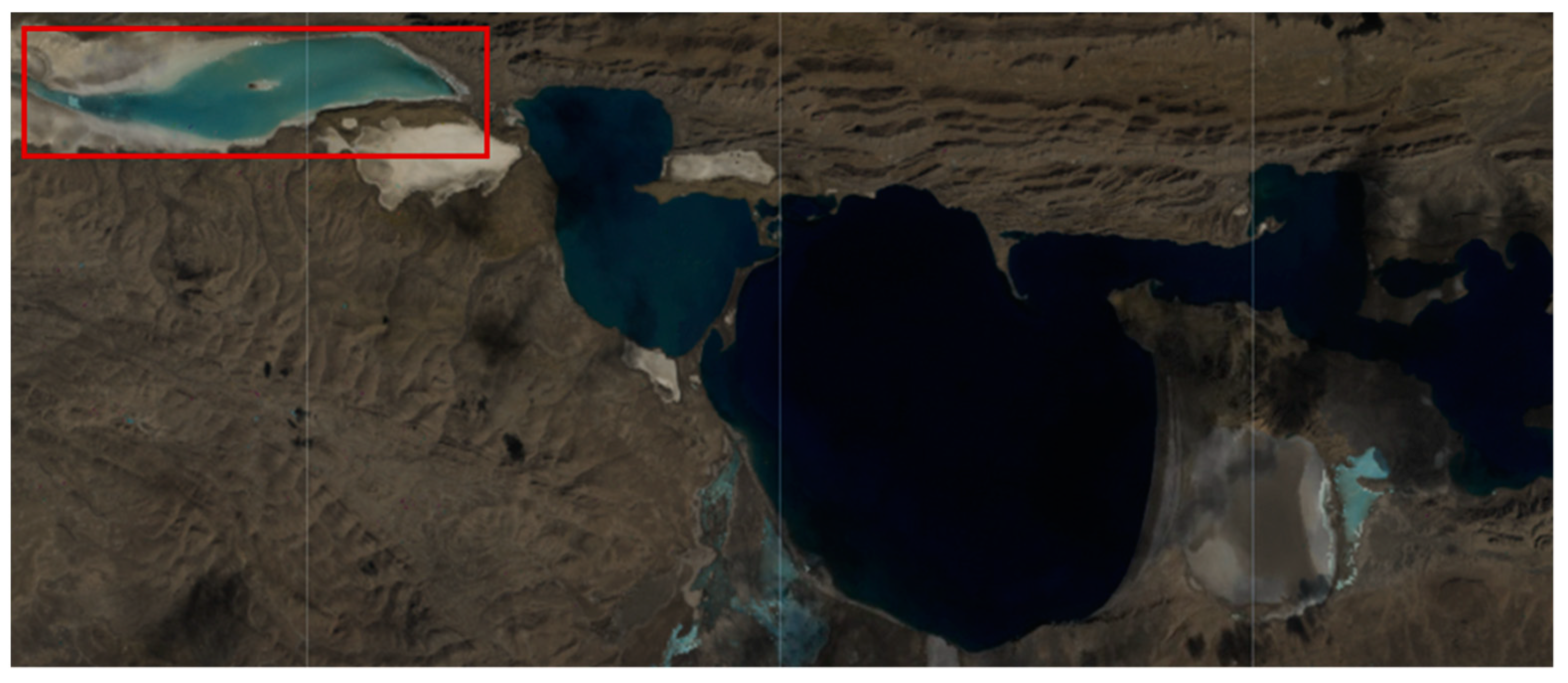
In our method, all the edges found by the Canny edge detector were used to find a suitable NDWI thresholds. However, some lakes may consist of several waterbodies with distinguish water characteristics among them. As such, it is difficult to extract all the waterbodies using a single threshold. As shown in Figure 23, the water body in the red frame, which is a part of the large lake, is shallow, has a low NDWI value, and cannot be extracted with other waterbodies of the lake using the same threshold. Future improvement should try to identify disconnected waterbodies of a lake and then find the adaptive thresholds for individual parts.
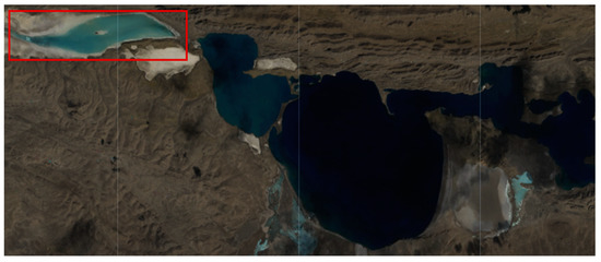
Figure 23.
Composite images, detected water extents and NDWI thresholds for lake Ganju Lake in different years (t is the NDWI threshold).
4.4. Lake Area Change and Climate Variables
The overall lake area has shown an increasing trend in the past 30 years, and Mann–Kendall trend analysis indicates a significant increase trend. The analysis also shows that the change points are mostly concentrated between 2003 and 2006 (see Section 3.2). The main difference before and after change point is that the area before the change point increases faster, while the area after the change point slows down. It can be seen from the results that the lake area has a decreasing trend between 1990 and 1995. This trend has also been noted by other researchers [18]. Intuitively, 1995 should also be a change point, but Pettitt method did not identify it. Lei, Y. et al. (2014) and Zhang, Z. et al. (2018) also used the Mann–Kendall to study lake area changes in the Qinghai-Tibet Plateau, and their results indicated a change point around 2000 [60]. The reason for this difference may be that a large number of small lakes with an area of less than 10 km2 were used in this study. These lakes were not used in previous studies, and their change points are slightly lagging behind large lakes.
Regarding the reasons for the change of lake area in this region, studies have shown that climate change after 2000 led to significant increase in precipitation and temperature, thereby affecting lake area [60]. Some studies have pointed out that the increase in lake water may be caused by melting glaciers which accounts for at least 20%, and even 100% in some areas [61]. Liu, X. et al. (2021) also pointed out that the intensification of ISM can also significantly increase lake water volume in the area [62]. As far as this research is concerned, there are many factors that may affect lake area, and the contribution rates of different factors are still unclear, thus further research is needed.
In this research, the relationship between lake area and climate is mainly explored through correlation analysis, which has certain limitations in understanding the driving factors of lake area change. We know that lake area in the southern part of the IB has a high and significant correlation with temperature. For example, Wang, X. et al. (2013) showed a correlation of 0.81 between decreasing glacier area and increasing lake numbers and extent in the TP over the past 40 years [4]. However, we still do not know how the temperature affects lake area through the physical processes such as melting glaciers and frozen soil or the change of evapotranspiration, as well as the contributions from each process [12,20,63,64]. To fully understand the driving forces, it is necessary to estimate lake water volume change and quantify the precipitation, surface runoff, evapotranspiration, glacier melting and other hydrological variables. This is a separate piece of research that we are currently conducting, and related manuscripts are in preparation.
We use the years in which the El Niño/La Niña events existed to study the relationship between the El Niño/La Niña events and lake area change. However, the duration of El Nino/La Nina events varies. It may start in spring or fall, and the outbreak may span two or more years [65]. As such, there is a deviation between the actual years El Niño/La Niña events existed and the El Niño/La Niña years used in our analysis, which may lead to uncertainty in the results. In addition, some studies have shown that there may have a time lag in the impact of El Niño event on precipitation in China. For example, in the summer of the following year after El Niño/La Niña events, floods (droughts) are more likely to occur in the middle and lower reaches of the Yangtze River, while droughts (floods) are more likely to occur in southern China [66]. Whether there is a time lag between El Niño/La Niña events and lake area change in the TP remains to be further investigated.
5. Conclusions
Using Landsat imagery and cloud-based geospatial analysis platform GEE, this study identified and calculated annual area for all the lakes greater than 1 km2 in the BETP from 1990 to 2019. Results show that total lake area in the study area expanded significantly with an increasing rate of 451.19 km2·year−1. Most lakes expanded rapidly from 1990 to 2005, and the expansion rate slowed down from 2005 to 2019.
The study also examined the relationships between lake area and local (temperature and precipitation), regional (EASM and ISM) and global (NAO, AMO and El Niño/La Niña events) climatic variables and atmospheric and ocean circulations at three spatial scales. In the past 30 years, local precipitation and temperature in the EBTP generally showed an upward trend. Our results show that the correlation between lake area and precipitation gradually weakened from west to east in the EBTP, and the sub-regions where lake area is significantly correlated with temperature are mainly located in the central and southern IB and the entire QB. For regional monsoon systems, there is no significant correlation between EASM and lake area, though ISM has some correlation with the lake area in western sub-regions of the IB. For global atmospheric circulations, lake area has a significant connection with AMO but has no correlation with NAO. In addition, we found abnormal drought (rainfall) brought by the El Niño/La Niña events is significantly correlated with lake area change in most sub-regions in the IB. There are still limitations in our lake identification methods and in the correlation analysis, and we will continue improving the methods and exploring the driving forces of lake change in the EBTP.
Author Contributions
Conceptualization, L.Z., X.L. and J.S.; methodology, X.L.; software, M.L.; validation, J.W., M.L. and L.W.; formal analysis, M.L.; investigation, L.W.; resources, J.W.; writing—original draft preparation, M.L.; writing—review and editing, J.W.; visualization, M.L.; supervision, X.L.; project administration, J.W.; funding acquisition, L.Z. All authors have read and agreed to the published version of the manuscript.
Funding
Please add: This research work was supported by the Strategic Priority Research Program [grant no. XDA20020100) of the Chinese Academy of Science, the Open Fund Project of the Key Laboratory of Coastal Zone Exploitation and Protection, Ministry of Natural Resources [grant no. 2019CZEPK01)] and the Natural Science Foundation of the Higher Education Institutions of Jiangsu Province, China [grant no. 21KJB170010)].
Institutional Review Board Statement
Not applicable.
Informed Consent Statement
Not applicable.
Data Availability Statement
The lake area data in this paper are freely available at https://doi.org/10.5281/zenodo.4781832 (accessed on 24 September 2021).
Conflicts of Interest
The authors declare no conflict of interest.
References
- Song, C.; Huang, B.; Richards, K.; Ke, L.; Hien Phan, V. Accelerated lake expansion on the Tibetan Plateau in the 2000s: Induced by glacial melting or other processes? Water Resour. Res. 2014, 50, 3170–3186. [Google Scholar] [CrossRef] [Green Version]
- Yanai, M.; Li, C.; Song, Z. Seasonal heating of the Tibetan Plateau and its effects on the evolution of the Asian summer monsoon. J. Meteorol. Soc. Japan. Ser. II 1992, 70, 319–351. [Google Scholar] [CrossRef] [Green Version]
- Yanai, M.; Li, C. Mechanism of Heating and the Boundary Layer over the Tibetan Plateau. Mon. Weather Rev. 1994, 122, 305. [Google Scholar] [CrossRef]
- Wang, X.; Siegert, F.; Zhou, A.-G.; Franke, J. Glacier and glacial lake changes and their relationship in the context of climate change, Central Tibetan Plateau 1972–2010. Glob. Planet Chang. 2013, 111, 246–257. [Google Scholar] [CrossRef]
- You, Q.; Kang, S.; Flügel, W.-A.; Sanchez-Lorenzo, A.; Yan, Y.; Xu, Y.; Huang, J. Does a weekend effect in diurnal temperature range exist in the eastern and central Tibetan Plateau? Environ. Res. Lett 2009, 4, 045202. [Google Scholar] [CrossRef]
- Zhou, X.; Liu, X.; Zhang, Z. Automatic Extraction of Lakes on the Qinghai-Tibet Plateau from Sentinel-1 SAR Images. In Proceedings of the 2019 SAR in Big Data Era (BIGSARDATA), Beijing, China, 5–6 August 2019; pp. 1–4. [Google Scholar]
- Wan, W.; Long, D.; Hong, Y.; Ma, Y.; Yuan, Y.; Xiao, P.; Duan, H.; Han, Z.; Gu, X. A lake data set for the Tibetan Plateau from the 1960s, 2005, and 2014. Sci. Data 2016, 3, 160039. [Google Scholar] [CrossRef] [PubMed] [Green Version]
- Adrian, R.; O’Reilly, C.M.; Zagarese, H.; Baines, S.B.; Hessen, D.O.; Keller, W.; Livingstone, D.M.; Sommaruga, R.; Straile, D.; Van Donk, E. Lakes as sentinels of climate change. Limnol. Oceanogr. 2009, 54, 2283–2297. [Google Scholar] [CrossRef] [PubMed]
- Zhang, G.; Yao, T.; Shum, C.; Yi, S.; Yang, K.; Xie, H.; Feng, W.; Bolch, T.; Wang, L.; Behrangi, A. Lake volume and groundwater storage variations in Tibetan Plateau’s endorheic basin. Geophys. Res. Lett. 2017, 44, 5550–5560. [Google Scholar] [CrossRef]
- Dyurgerov, M.B.; Meier, M.F. Glaciers and the Changing Earth System: A 2004 Snapshot; Institute of Arctic and Alpine Research, University of Colorado Boulder: Boulder, CO, USA, 2005; Volume 58. [Google Scholar]
- Yang, K.; Wu, H.; Qin, J.; Lin, C.; Tang, W.; Chen, Y. Recent climate changes over the Tibetan Plateau and their impacts on energy and water cycle: A review. Glob. Planet Chang. 2014, 112, 79–91. [Google Scholar] [CrossRef]
- Zhan, P.; Song, C.; Wang, J.; Li, W.; Ke, L.; Liu, K.; Chen, T. Recent Abnormal Hydrologic Behavior of Tibetan Lakes Observed by Multi-Mission Altimeters. Remote Sens. 2020, 12, 2986. [Google Scholar] [CrossRef]
- Liu, X.; Chen, B. Climatic warming in the Tibetan Plateau during recent decades. Int. J. Climatol. A J. R. Meteorol. Soc. 2000, 20, 1729–1742. [Google Scholar] [CrossRef]
- Lin, C.; Yang, K.; Qin, J.; Fu, R. Observed coherent trends of surface and upper-air wind speed over China since 1960. J. Clim. 2013, 26, 2891–2903. [Google Scholar] [CrossRef] [Green Version]
- Zhang, X.; Ren, Y.; Yin, Z.Y.; Lin, Z.; Zheng, D. Spatial and temporal variation patterns of reference evapotranspiration across the Qinghai-Tibetan Plateau during 1971–2004. J. Geophys. Res. Atmos. 2009, 114, D15105. [Google Scholar] [CrossRef]
- Zhang, C.; Tang, Q.; Chen, D.; van der Ent, R.J.; Liu, X.; Li, W.; Haile, G.G. Moisture source changes contributed to different precipitation changes over the northern and southern Tibetan Plateau. J. Hydrometeorol. 2019, 20, 217–229. [Google Scholar] [CrossRef]
- Lei, Y.; Yang, K.; Wang, B.; Sheng, Y.; Bird, B.W.; Zhang, G.; Tian, L. Response of inland lake dynamics over the Tibetan Plateau to climate change. Clim. Chang. 2014, 125, 281–290. [Google Scholar] [CrossRef]
- Zhang, G.; Luo, W.; Chen, W.; Zheng, G. A robust but variable lake expansion on the Tibetan Plateau. Sci. Bull. 2019, 64, 1306–1309. [Google Scholar] [CrossRef] [Green Version]
- Liao, J.; Shen, G.; Li, Y. Lake variations in response to climate change in the Tibetan Plateau in the past 40 years. Int. J. Digit. Earth 2013, 6, 534–549. [Google Scholar] [CrossRef]
- Yang, K.; Yao, F.; Wang, J.; Luo, J.; Shen, Z.; Wang, C.; Song, C. Recent dynamics of alpine lakes on the endorheic Changtang Plateau from multi-mission satellite data. J. Hydrol. 2017, 552, 633–645. [Google Scholar] [CrossRef]
- Yao, F.; Wang, J.; Yang, K.; Wang, C.; Walter, B.A.; Crétaux, J.-F. Lake storage variation on the endorheic Tibetan Plateau and its attribution to climate change since the new millennium. Environ. Res. Lett 2018, 13, 064011. [Google Scholar] [CrossRef]
- Zhang, G.; Bolch, T.; Chen, W.; Crétaux, J.-F. Comprehensive estimation of lake volume changes on the Tibetan Plateau during 1976–2019 and basin-wide glacier contribution. Sci. Total Environ. 2021, 772, 145463. [Google Scholar] [CrossRef]
- Pekel, J.-F.; Cottam, A.; Gorelick, N.; Belward, A.S. High-resolution mapping of global surface water and its long-term changes. Nature 2016, 540, 418–422. [Google Scholar] [CrossRef] [PubMed]
- Song, C.; Huang, B.; Ke, L. Modeling and analysis of lake water storage changes on the Tibetan Plateau using multi-mission satellite data. Remote Sens. Environ. 2013, 135, 25–35. [Google Scholar] [CrossRef]
- Ke, L.; Ding, X.; Li, W.; Qiu, B. Remote sensing of glacier change in the central Qinghai-Tibet Plateau and the relationship with changing climate. Remote Sens. 2017, 9, 114. [Google Scholar] [CrossRef] [Green Version]
- Feng, L.; Zhou, T. Water vapor transport for summer precipitation over the Tibetan Plateau: Multidata set analysis. J. Geophys. Res. Atmos. 2012, 117. [Google Scholar] [CrossRef] [Green Version]
- Li, Y.; Su, F.; Chen, D.; Tang, Q. Atmospheric water transport to the endorheic Tibetan plateau and its effect on the hydrological status in the region. J. Geophys. Res. Atmos. 2019, 124, 12864–12881. [Google Scholar] [CrossRef]
- Chang, X.; Wang, B.; Yan, Y.; Hao, Y.; Zhang, M. Characterizing effects of monsoons and climate teleconnections on precipitation in China using wavelet coherence and global coherence. Clim. Dynam. 2019, 52, 5213–5228. [Google Scholar] [CrossRef] [Green Version]
- Yao, T.; Thompson, L.; Yang, W.; Yu, W.; Gao, Y.; Guo, X.; Yang, X.; Duan, K.; Zhao, H.; Xu, B. Different glacier status with atmospheric circulations in Tibetan Plateau and surroundings. Nat. Clim. Chang. 2012, 2, 663–667. [Google Scholar] [CrossRef]
- Yao, T.; Masson-Delmotte, V.; Gao, J.; Yu, W.; Yang, X.; Risi, C.; Sturm, C.; Werner, M.; Zhao, H.; He, Y. A review of climatic controls on δ18O in precipitation over the Tibetan Plateau: Observations and simulations. Rev. Geophys. 2013, 51, 525–548. [Google Scholar] [CrossRef]
- Lei, Y.; Zhu, Y.; Wang, B.; Yao, T.; Yang, K.; Zhang, X.; Zhai, J.; Ma, N. Extreme lake level changes on the Tibetan Plateau associated with the 2015/2016 El Niño. Geophys. Res. Lett. 2019, 46, 5889–5898. [Google Scholar] [CrossRef]
- Zhang, G.; Yao, T.; Xie, H.; Kang, S.; Lei, Y. Increased mass over the Tibetan Plateau: From lakes or glaciers? Geophys. Res. Lett. 2013, 40, 2125–2130. [Google Scholar] [CrossRef]
- Zhang, G.; Yao, T.; Xie, H.; Zhang, K.; Zhu, F. Lakes’ state and abundance across the Tibetan Plateau. Chin. Sci. Bull. 2014, 59, 3010–3021. [Google Scholar] [CrossRef]
- Beck, H.E.; Zimmermann, N.E.; McVicar, T.R.; Vergopolan, N.; Berg, A.; Wood, E.F. Present and future Köppen-Geiger climate classification maps at 1-km resolution. Sci. Data 2018, 5, 180214. [Google Scholar] [CrossRef] [PubMed] [Green Version]
- Lehner, B.; Verdin, K.; Jarvis, A. New global hydrography derived from spaceborne elevation data. Eos Trans. Am. Geophys. Union 2008, 89, 93–94. [Google Scholar] [CrossRef]
- Gorelick, N.; Hancher, M.; Dixon, M.; Ilyushchenko, S.; Thau, D.; Moore, R. Google Earth Engine: Planetary-scale geospatial analysis for everyone. Remote Sens. Environ. 2017, 202, 18–27. [Google Scholar] [CrossRef]
- He, J.; Yang, K.; Tang, W.; Lu, H.; Qin, J.; Chen, Y.; Li, X. The first high-resolution meteorological forcing dataset for land process studies over China. Sci. Data 2020, 7, 25. [Google Scholar] [CrossRef] [PubMed] [Green Version]
- Yang, K.; He, J.; Tang, W.; Qin, J.; Cheng, C.C. On downward shortwave and longwave radiations over high altitude regions: Observation and modeling in the Tibetan Plateau. Agric. For. Meteorol. 2010, 150, 38–46. [Google Scholar] [CrossRef]
- Yang, K.; He, J. China meteorological forcing dataset (1979–2018); National Tibetan Plateau Data Center: Beijing, China, 2018. [Google Scholar] [CrossRef]
- Sun, S.; Chen, B.; Ge, M.; Qu, J.; Che, T.; Zhang, H.; Lin, X.; Che, M.; Zhou, Z.; Guo, L. Improving soil organic carbon parameterization of land surface model for cold regions in the Northeastern Tibetan Plateau, China. Ecol. Model. 2016, 330, 1–15. [Google Scholar] [CrossRef] [Green Version]
- Wang, B.; Wu, R.; Lau, K. Interannual variability of the Asian summer monsoon: Contrasts between the Indian and the western North Pacific–East Asian monsoons. J. Clim. 2001, 14, 4073–4090. [Google Scholar] [CrossRef]
- Li, J.; Zeng, Q. A unified monsoon index. Geophys. Res. Lett. 2002, 29, 115-1–115-4. [Google Scholar] [CrossRef]
- Enfield, D.B.; Mestas-Nuñez, A.M.; Trimble, P.J. The Atlantic multidecadal oscillation and its relation to rainfall and river flows in the continental US. Geophys. Res. Lett. 2001, 28, 2077–2080. [Google Scholar] [CrossRef] [Green Version]
- Hurrell, J.W. Decadal trends in the North Atlantic Oscillation: Regional temperatures and precipitation. Science 1995, 269, 676–679. [Google Scholar] [CrossRef] [PubMed] [Green Version]
- Ninglian, W.; Thompson, L.; Davis, M.; Mosley-Thompson, E.; Tandong, Y.; Jianchen, P. Influence of variations in NAO and SO on air temperature over the northern Tibetan Plateau as recorded by δ18O in the Malan ice core. Geophys. Res. Lett. 2003, 30. [Google Scholar] [CrossRef]
- Gao, B. NDWI—A normalized difference water index for remote sensing of vegetation liquid water from space. Remote Sens. Environ. 1996, 58, 257–266. [Google Scholar] [CrossRef]
- McFeeters, S.K. The use of the Normalized Difference Water Index (NDWI) in the delineation of open water features. Int. J. Remote Sens. 1996, 17, 1425–1432. [Google Scholar] [CrossRef]
- Li, W.; Du, Z.; Ling, F.; Zhou, D.; Wang, H.; Gui, Y.; Sun, B.; Zhang, X. A comparison of land surface water mapping using the normalized difference water index from TM, ETM+ and ALI. Remote Sens. 2013, 5, 5530–5549. [Google Scholar] [CrossRef] [Green Version]
- Yang, K.; Li, M.; Liu, Y.; Cheng, L.; Duan, Y.; Zhou, M. River delineation from remotely sensed imagery using a multi-scale classification approach. IEEE J. Sel. Top. Appl. Earth Obs. Remote Sens. 2014, 7, 4726–4737. [Google Scholar] [CrossRef]
- Donchyts, G.; Schellekens, J.; Winsemius, H.; Eisemann, E.; Van de Giesen, N. A 30 m resolution surface water mask including estimation of positional and thematic differences using landsat 8, srtm and openstreetmap: A case study in the Murray-Darling Basin, Australia. Remote Sens. 2016, 8, 386. [Google Scholar] [CrossRef] [Green Version]
- Hamed, K.H.; Rao, A.R. A modified Mann-Kendall trend test for autocorrelated data. J. Hydrol. 1998, 204, 182–196. [Google Scholar] [CrossRef]
- Crétaux, J.-F.; Jelinski, W.; Calmant, S.; Kouraev, A.; Vuglinski, V.; Bergé-Nguyen, M.; Gennero, M.-C.; Nino, F.; Del Rio, R.A.; Cazenave, A. SOLS: A lake database to monitor in the Near Real Time water level and storage variations from remote sensing data. Adv. Space Res. 2011, 47, 1497–1507. [Google Scholar] [CrossRef]
- Chen, C.; Twycross, J.; Garibaldi, J.M. A new accuracy measure based on bounded relative error for time series forecasting. PLoS ONE 2017, 12, e0174202. [Google Scholar] [CrossRef] [Green Version]
- Bian, H.; Li, W.; Li, Y.; Ren, B.; Niu, Y.; Zeng, Z. Driving forces of changes in China’s wetland area from the first (1999–2001) to second (2009–2011) National Inventory of Wetland Resources. Glob. Ecol. Conserv. 2020, 21, e00867. [Google Scholar] [CrossRef]
- Pettitt, A. A non-parametric approach to the change-point problem. J. R. Stat. Soc. Ser. C (Appl. Stat.) 1979, 28, 126–135. [Google Scholar] [CrossRef]
- Ryberg, K.R.; Hodgkins, G.A.; Dudley, R.W. Change points in annual peak streamflows: Method comparisons and historical change points in the United States. J. Hydrol. 2020, 583, 124307. [Google Scholar] [CrossRef]
- Bingyi, W. Weakening of Indian summer monsoon in recent decades. Adv. Atmos. Sci. 2005, 22, 21–29. [Google Scholar] [CrossRef]
- Sun, J.; Yang, K.; Guo, W.; Wang, Y.; He, J.; Lu, H. Why has the Inner Tibetan Plateau become wetter since the mid-1990s? J. Clim. 2020, 33, 8507–8522. [Google Scholar] [CrossRef]
- Hwang, C.; Peng, M.-F.; Ning, J.; Luo, J.; Sui, C.-H. Lake level variations in China from TOPEX/Poseidon altimetry: Data quality assessment and links to precipitation and ENSO. Geophys. J. Int. 2005, 161, 1–11. [Google Scholar] [CrossRef] [Green Version]
- Zhang, Z.; Chang, J.; Xu, C.-Y.; Zhou, Y.; Wu, Y.; Chen, X.; Jiang, S.; Duan, Z. The response of lake area and vegetation cover variations to climate change over the Qinghai-Tibetan Plateau during the past 30 years. Sci. Total Environ. 2018, 635, 443–451. [Google Scholar] [CrossRef]
- Qiao, B.; Zhu, L.; Yang, R. Temporal-spatial differences in lake water storage changes and their links to climate change throughout the Tibetan Plateau. Remote Sens. Environ. 2019, 222, 232–243. [Google Scholar] [CrossRef]
- Liu, X.; Madsen, D.; Zhang, X. The Driving Forces Underlying Spatiotemporal Lake Extent Changes in the Inner Tibetan Plateau During the Holocene. Front. Earth Sci. 2021, 9, 685928. [Google Scholar]
- Zhao, Z.; Liu, F.; Zhang, Y.; Liu, L.; Qi, W. The dynamic response of lakes in the Tuohepingco Basin of the Tibetan Plateau to climate change. Environ. Earth Sci. 2017, 76, 137. [Google Scholar] [CrossRef]
- Zhao, Z.; Zhang, Y.; Liu, L.; Liu, F.; Zhang, H. Recent changes in wetlands on the Tibetan Plateau: A review. J. Geogr. Sci. 2015, 25, 879–896. [Google Scholar] [CrossRef] [Green Version]
- Chen, H.; Xu, F.; Li, X.; Xia, T.; Zhang, Y. Intensities and time-frequency variability of ENSO in the last 65 years. J. Trop. Meteorol. 2017, 33, 683–694. (In Chinese) [Google Scholar] [CrossRef]
- Li, C.; Li, X.; Liu, Y.; Pan, W. Impact of spring and summer onset type ENSO on summer precipitation in China. Clim. Environ. Res. 2016, 21, 258–268. (In Chinese) [Google Scholar]


Publisher’s Note: MDPI stays neutral with regard to jurisdictional claims in published maps and institutional affiliations. |
© 2021 by the authors. Licensee MDPI, Basel, Switzerland. This article is an open access article distributed under the terms and conditions of the Creative Commons Attribution (CC BY) license (https://creativecommons.org/licenses/by/4.0/).