Small-Sized Ship Detection Nearshore Based on Lightweight Active Learning Model with a Small Number of Labeled Data for SAR Imagery

Abstract

Marine ship detection by synthetic aperture radar (SAR) is an important remote sensing technology. The rapid development of big data and artificial intelligence technology has facilitated the wide use of deep learning methods in SAR imagery for ship detection. Although deep learning can achieve a much better detection performance than traditional methods, it is difficult to achieve satisfying performance for small-sized ships nearshore due to the weak scattering caused by their material and simple structure. Another difficulty is that a huge amount of data needs to be manually labeled to obtain a reliable CNN model. Manual labeling each datum not only takes too much time but also requires a high degree of professional knowledge. In addition, the land and island with high backscattering often cause high false alarms for ship detection in the nearshore area. In this study, a novel method based on candidate target detection, boundary box optimization, and convolutional neural network (CNN) embedded with active learning strategy is proposed to improve the accuracy and efficiency of ship detection in nearshore areas. The candidate target detection results are obtained by global threshold segmentation. Then, the strategy of boundary box optimization is defined and applied to reduce the noise and false alarms caused by island and land targets as well as by sidelobe interference. Finally, a lightweight CNN embedded with active learning scheme is used to classify the ships using only a small labeled training set. Experimental results show that the performance of the proposed method for small-sized ship detection can achieve 97.78% accuracy and 0.96 F1-score with Sentinel-1 images in complex nearshore areas.

1. Introduction

Ship detection in SAR images plays a vital role in marine transportation and dynamic surveillance applications. Therefore, monitoring marine activity quickly and efficiently by the use of the remote sensing technique, which can be used to observe the Earth at a large scale, is important. Compared with optical remote sensing, SAR as an active remote sensing technique is an adequate approach for ship detection, as it is not only sensitive to water and hard targets but also works during daytime and nighttime, and in all weather conditions [1,2]. Fortunately, many SAR satellites, such as RADARSAT-1/2, TerraSAR-X, Sentinel-1A/B, ALOS-PALSAR, COSMO-SkyMed, and Gaofen-3, have been successfully launched in recent years, and are now providing many images in different modes and polarizations for maritime applications and ship detection.

In the previous studies, constant false alarm rate (CFAR), as a classical target detection method, has been usually used for ship detection [3,4,5]. However, applying a sliding window when processing SAR images by CFAR is necessary. Moreover, the setting of the protection and background window sizes not only affects the detection result but also takes a long time. The development and success of artificial intelligence have contributed to the tremendous application of convolutional neural networks (CNNs) [6], such as object recognition, image classification, and automatic object clustering. In the field of object recognition, the detection methods based on CNN can be classified into two categories (1): single-stage detectors such as SDD, Yolov1/v2v3/v4, and RetinaNet; and (2) two-stage detectors such as R-CNN, Fast R-CNN, Faster R-CNN, and Mask-RCNN. Although they achieve satisfactory results in natural images, direct transfer to SAR images for ship detection tasks is difficult. The primary reason is due to the different characteristics of the objects; for example, objects are mostly centrally located in natural images, while ships are multi-scale and randomly distributed in SAR images. Some studies have focused on the detection of ships in SAR images based on deep learning methods [7,8]. A public dataset called the SAR Ship Detection Dataset was constructed using different SAR images to make the CNN detector suitable for ship detection in SAR images [7]. Then, the Faster R-CNN method was improved by fusion features and achieved a good performance, which demonstrated that CNN detectors could be used for SAR image ship [7]. A large size dataset with different SAR sensor images was also constructed for ship detection under complex backgrounds, the result showed the RetinaNet detector could reach the accuracy of 91.36%. [8]. Single shot multibox detector (SSD) was modified by removing three layers to detect the ship. Although the number of the parameters in SSD was decreased, the accuracy only slightly increased. A feature pyramid network (FPN) was used to address various scales of interesting objects. Compared with Faster RCNN and SSD, the average accuracy had a significant improvement [9]. Chen et al. [10] proposed a novel CNN network for detecting multi-scale ships in complex scenes by taking advantage of the attention mechanism. Cui et al. [11] designed a feature pyramid network integrating dense attention mechanisms; the proposed method proved to be suitable for multi-scale ship detection. A receptive pyramid network extraction strategy and attention mechanism technology were also proven to be effective in the ship detection task, but the processing efficiency was low due to the complex model structure [12]. The fusion feature extractor network was used to generate proposals from fusing feature maps in a bottom-up and top-down method to detect ships. Although the ship detection-based CNN had been applied to SAR images, the small and inshore targets under complex backgrounds remained difficult [13,14]. There were still some missing ships and false alarms due to the similarity in shape and intensity between ships and some building and harbor facilities [13]. Several state-of-art detectors were applied for ship detection, the accuracy of Faster R-CNN, Mask R-CNN, RetinaNet was more than 88% under the bounding box IoU threshold of 0.5, but the poor performance was observed in small ships [14]. The FPN module and k-means anchor boxes were integrated into SSD backbones, and the results demonstrated that the rate of false detections and misses of target ship also decreased in the case of small-object ship recognition [15]. An attention-oriented balanced pyramid was proposed to semantically balance the multiple features at different levels, in order to focus more attention on the small ships [16]. Multi-network was used for target detection to increase the accuracy of small-scale ship detection. The salient feature map and SAR image were input into two networks to train the CNN detectors, the accuracy of small ships could reach 75.35% [17]. The detector-based CNN models were often designed to be excessively complex in order to detect small ship targets, thus, the efficiency and accuracy cannot be balanced. Multi-network and two-stage detection methods were proposed to simplify the CNN model structure and decrease the false alarm of candidate detection, but the auxiliary data and a large number of labeled training samples need to be prepared before inputting them into the CNN network [17]. A method of candidates’ rough detection network and ship identifying network was used to realize fast ship detection [18]. A two-stage ship detection method was proposed; however, the interpretability of the model was not addressed [19]. Then, the visual feature was analyzed, and the accuracy of small ships was improved by two-stage ship detection [20]. Although the above-mentioned models have been widely used in weak and small target detection, they have difficulty achieving satisfying performance due to the fact that most of the small-sized ships are nonmetallic fishing boats, and that generating strong dihedral angle scattering is hard due to their simple structure, material, and target wobble [21]. Another difficulty is that a large amount of labeled data is required to obtain a reliable model. Manual labeling each sample datum not only takes too much time but also requires a high degree of professional knowledge. The ocean surface waves, surface wind, upwelling, surface currents, eddies, and sea state can modulate and influence the ocean surface; thus, the SAR image is relatively complex in the ocean areas [22,23]. Therefore, manually labeling all samples of ships in different conditions is difficult. By labeling more annotated data, the quality of deep neural networks can be optimized. The difficulty is that manually labeling all samples of ships in different conditions is limited. A new training strategy should be adopted to obtain a stable ship detection model with a small number of labeled data. Although CNN networks are data-driven, the quality of the data is as important as the quantity. If the dataset contains ambiguous examples that are difficult to label accurately, the effectiveness of the model will be reduced. Active learning models can automatically label data by selecting those that the model considers most optimal, update the model, and repeat the process until the results are sufficiently good. Thus, inspired by active learning [24,25,26], a model was proposed that asks humans to annotate data that it considers uncertain. Models trained by active learning strategy are not only faster to train but also can converge to a good final model by using fewer data. An uncertainty-based approach [27], a diversity-based approach [28], and expected model change [29] are three major ways to select the next batch to be labeled [24,30]. Various methods for applying active learning to deep networks have been proposed recently; however, almost all of them are either designed specifically for their target tasks or operationally inadequate for large networks.

In this study, an improved two-stage ship detection method by active learning scheme with a small number of labeled sample data is proposed. To begin with, an exponential inverse cumulative distribution function [20] is employed to estimate the segmentation threshold and obtain candidate detection results. Then, the candidate detection results are optimized by the rule of boundary box distance. Finally, the candidate detection results slices are input into the lightweight CNN with embedded active learning scheme to accurately recognize the ships by labeling a small number of training data.

The main contributions of this study are detailed as follows:

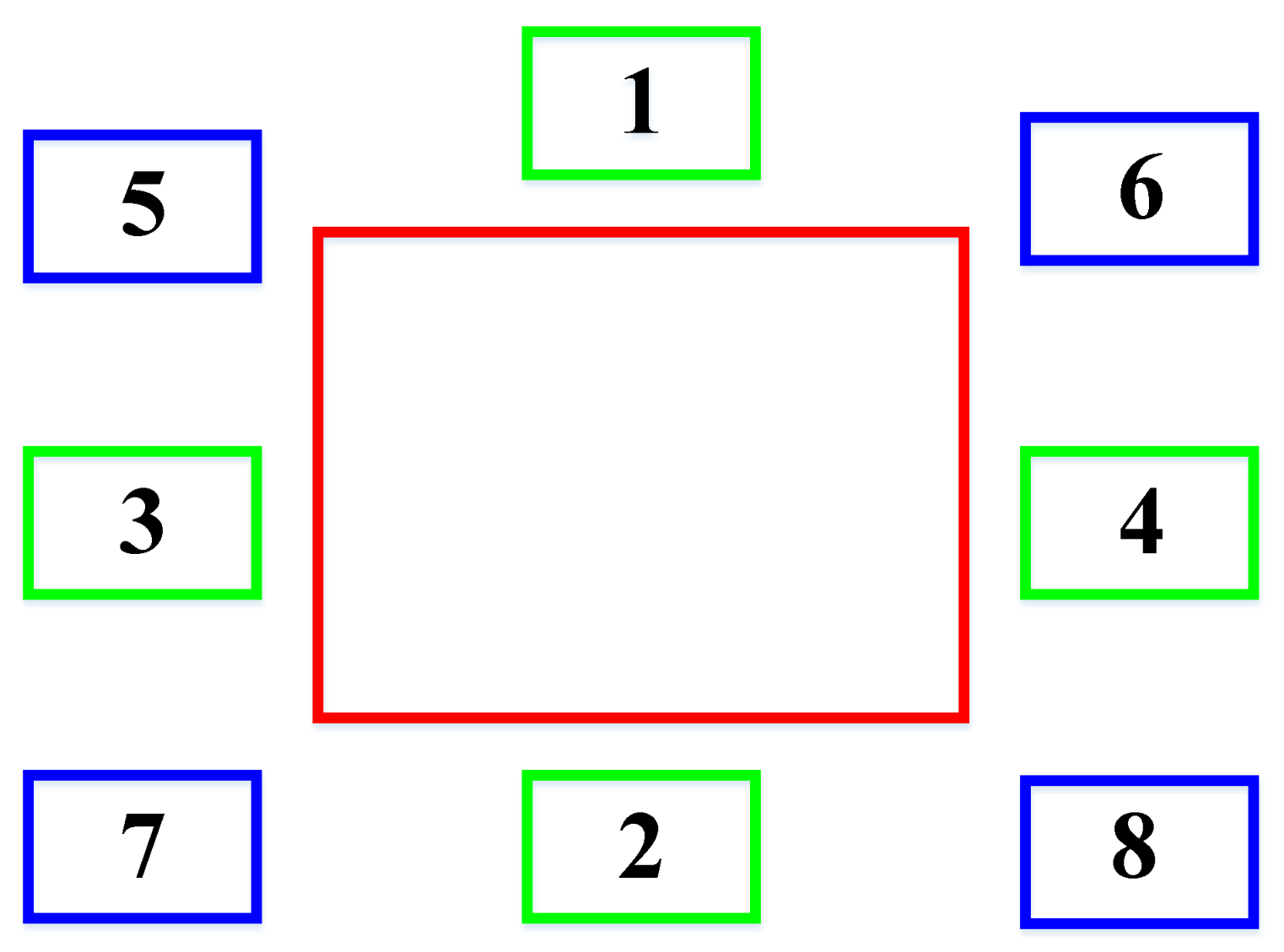
• The boundary box distance is proposed to optimize candidate targets further, which makes the boundaries of the candidate targets more reasonable;
• In the training stage, the proposed method can achieve better performance with a small number of labeled data;
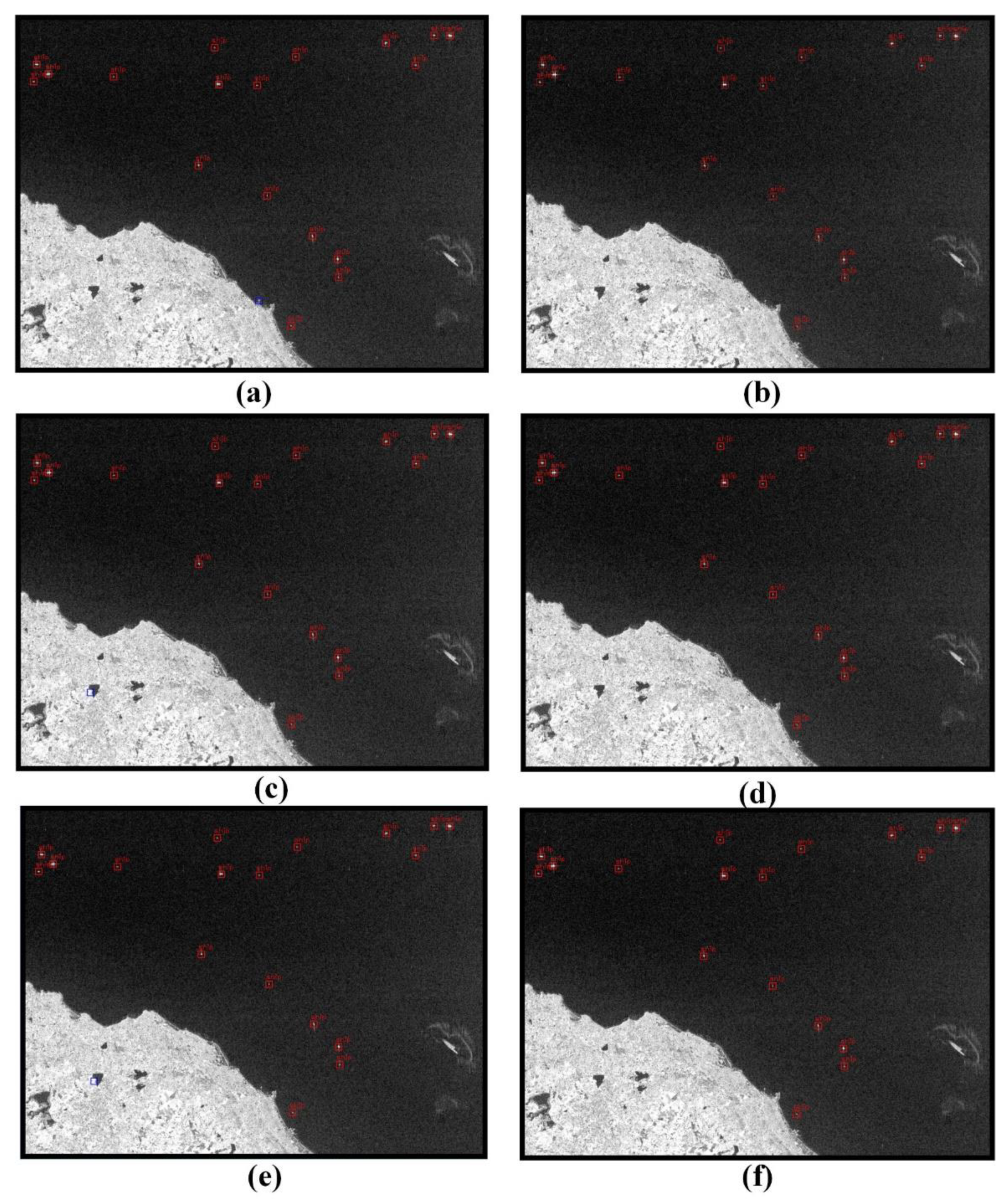
• In the ship detection stage, the proposed method is suitable for detecting a small-level ship on the nearshore.

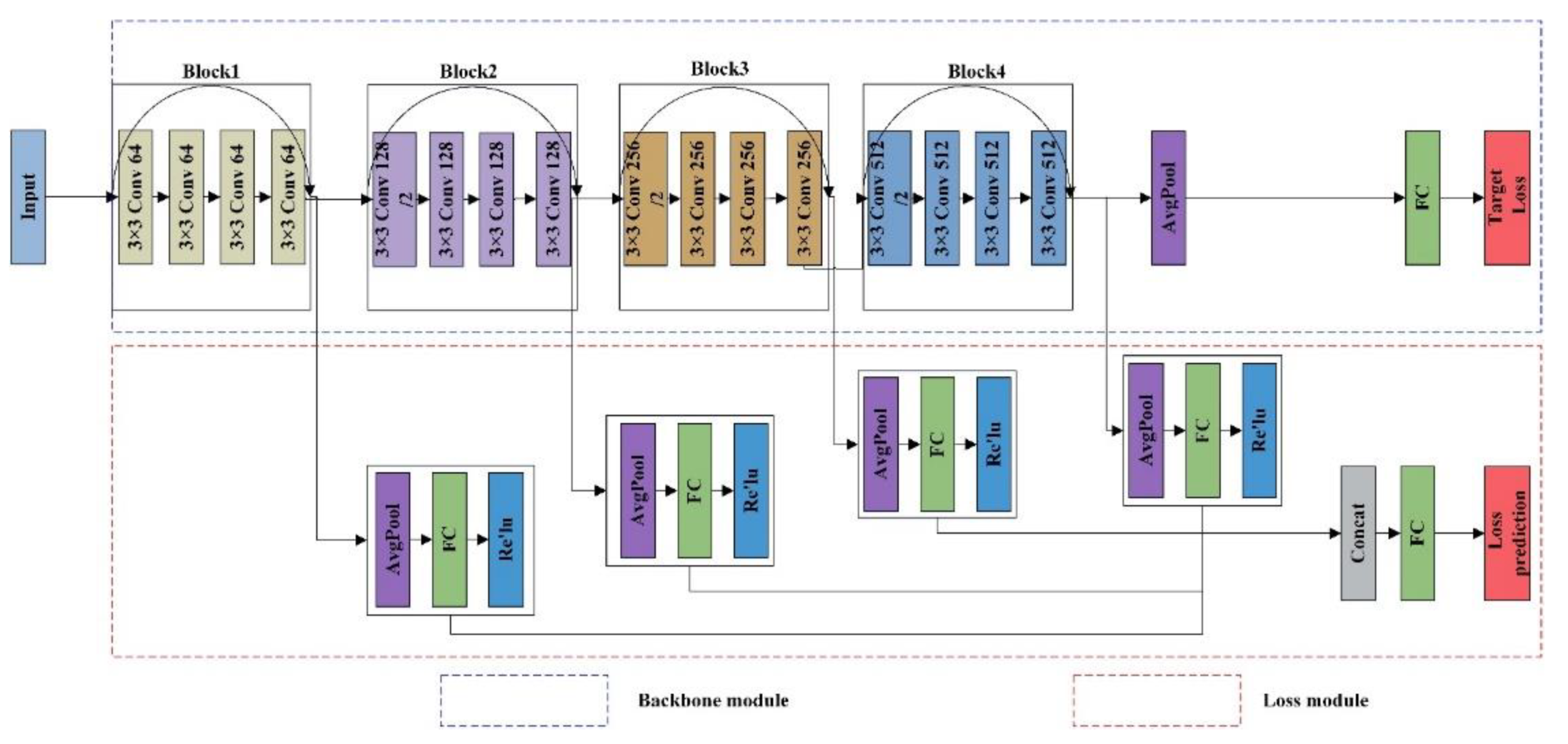
2. Methods

A strategy that combines deep learning with active learning is proposed, as shown in Figure 1, to reduce the volume of labeled training samples and the labeling cost for ship detection.

Figure 1 shows a typical example of a deep active learning model architecture. Algorithm 1 shows the training strategy. A huge number of unlabeled data $U_N$ is obtained. The subscript $N$ indicates a huge number of data samples. $K$ samples are randomly selected from the unlabeled pool and annotated manually. Then, an initially labeled dataset $L_K^0$ is constructed. We define the size of the unlabeled dataset pool as $U_{N-K}^0$. The subscript 0 refers to the initial stage. As soon as the initially labeled dataset $L_K^i$ is obtained, the loss function evaluates all the data in the unlabeled pool $U_{N-K}^i$ to obtain the data loss. The top-K data with the highest prediction loss are labeled and then added to the labeled training set. After $L_K^i$ is updated with the samples with the $K$ highest losses, it becomes $L_{2K}^i$, and the unlabeled pool is reduced and denoted as $U_{N-K}^i$ at the same time. This cycle is repeated until the label budget is exhausted [24,25,26].

Algorithm 1 pretraining of the proposed learning model

for cycles do

for i epoch do

if cycles == 0

Input: initial labeled data $L_k^0$ and unlabeled data $U_N$

else

1.  Train the lightweight CNN with embedded active learning scheme, and optimize it by stochastic gradient descent. The loss is calculated by target loss and loss prediction from the loss prediction module.        $Loss=L_{target}\left(y_t,\stackrel{\wedge }{y}\right)+\lambda \times L_{loss}\left(l_t,\stackrel{\wedge }{l}\right)$ 2.  Then, get the uncertainty with the data samples of the $k$ highest losses. 3.  Update the labeled dataset $L_{2K}^i$ and unlabeled dataset $U_{N-K}^i$, respectively.

end for

end for

The loss prediction module is the core to active learning for the task as the total loss defined in the model can be learned so as to imitate. This section describes how we design and improve the M-LeNet and ResNet models to make them suitable for active learning. The ResNet network architecture with residual learning framework has been proven to reduce the training error, converge quicky and avoid overfitting; hence, the ResNet18 was selected as the CNN baseline backbone target architectures [31]. The four convolution blocks of ResNet18 are selected as the loss prediction module. The size of the first convolution kernel size is changed from 5 to 3 to obtain detailed feature information in the ResNet18 network architecture. Figure 2 shows the improved ResNet18 contains the baseline target backbone (blue dashed rectangle box) and loss prediction module (red dashed rectangle box). The mid-level feature map blocks of the improved ResNet18 target backbone model are used as the input of the loss prediction module. Then, each feature map of the loss prediction module is connected by a global average pooling layer, a fully connected layer, and rectified linear unit layer. Finally, the total loss prediction could be obtained by concatenating target loss and prediction loss. The loss prediction module is much smaller and can learn jointly with the ResNet18 target backbone.

The performance of ship detection was once discussed in land-contained sea areas [19]. First, the candidate targets containing ships and false alarms were obtained by the CFAR method. Second, a dataset of 2286 ships and 2276 false alarms was constructed. Third, a CNN model was trained with constructed dataset and the final model was used to predict the ship [19]. Different from the candidate targets method in [19], a method based on exponential inverse cumulative distribution function was used to obtain candidate targets, which was proven to be faster and reasonable under different screens [20]. The low-complexity and lightweight M-LeNet was once proven to be effective for ship detection in the nearshore area [20]. Thus, the M-LeNet model in [20] is improved in the present study as the baseline backbone target module and loss prediction module in active learning, as shown in Figure 3. The two convolution blocks of M-LeNet are selected as loss prediction modules. The network contains two convolutional layers and has fewer parameters than the classical object detectors. Thus, the improved M-LeNet has a baseline backbone target module (blue dashed rectangle box) and a loss prediction module (red dashed rectangle box) consisting of blocks from the mid-level feature maps, as shown in Figure 3. Then, each feature map of the loss prediction module is connected by a global average pooling layer, a fully connected layer, and rectified linear unit. Finally, the total loss prediction could be obtained and jointly learned by concatenating target loss and prediction loss.

Given a training data point $x$, a backbone target module $f_{target}$, and a prediction module $f_{loss}$, the goal of active learning is to obtain the baseline backbone target prediction by $\stackrel{\wedge }{y}=f_{target}\left(x\right)$ and the prediction loss module by $\stackrel{\wedge }{l}=f_{loss}\left(h\right)$. $h$ is the mid-level feature map blocks of the improved ResNet18 or M-LeNet target backbone model. With the annotated data $y_t$ corresponding to the input data $x$, we can calculate the target loss by $l=L_{target}\left(y_t,\stackrel{\wedge }{y}\right)$ learning the target model. As the loss $l$ is a ground-truth target of $h$ for the loss prediction module, the loss of the prediction module can be obtained and computed by $L_{loss}\left(l,\stackrel{\wedge }{l}\right)$. Then, the final total loss function is defined as Equation (1), which could be jointly learned by the target backbone model and the loss prediction module [24].

$$Loss=L_{target}\left(y_t,\stackrel{\wedge }{y}\right)+\lambda \times L_{loss}\left(l,\stackrel{\wedge }{l}\right)$$

(1)

where λ is set to 1 in the experiment.

3. Results

3.1. Dataset

The dataset is constructed by Level-1 Sentinel-1 Ground Range Detected product data, located in the East China sea [20]. The performance of ship detection in VH polarization is better than VV polarization as the speckle-noise and false alarm of VV polarization can affect vessel-detection results more easily than cross-polarization [20,32]. Hence, the VH polarization image is used for ship detection. The training dataset comes from VH polarization and contains slices of 2099 false alarms and 1566 different scale ships, as listed in

Table 1. Number of Ships and false alarms.

Name	Count	Polarization
Ships	1566	VH
False alarms	2099

. The false alarms are mainly caused by bridges, lighthouses, buildings, small islands, reefs, and rocks, as well as ghosts caused by azimuth ambiguity, as shown in Figure 4a. The ship mainly has a different large size and a strong scattering intensity, as shown in Figure 4b. Figure 5 shows some Google Earth ground truth and the corresponding false alarm candidates.

Using the dataset constructed by [20], we train the lightweight CNN with embedded active learning scheme. Then, another two images located in the Qiongzhou Strait and the East China Sea are used for the candidate detection by data preprocessing and test the efficiency of the CNN with embedded active learning scheme with a few annotated training samples. The details of the SAR images, including the acquisition time, swath width, and imaging mode, are listed in

Table 2. Details of the Sentinel-1 images used in the experiments.

	Time (UTC)	Polarization	Resolution (m)	Swath (km)
1	12 January 2019, 09:53	VH,VV	10	250
2	7 December 2020, 10:48	VH,VV	10	250

.

3.2. Training Details

The experiments are conducted on a workstation that runs the Ubuntu 14.04 operating system, which is equipped with TITAN Xp GPU of 12 GB memory and Xeon W-2100 CPU of 32 RAM. We repeat the same experiment multiple times with different labeled sample datasets setting until the unlabeled datasets are exhausted for each active learning method. For each of the active learning cycles, we use stochastic gradient descent to optimize the baseline backbone and loss prediction module. The hyperparameters, such as initial learning rate, epochs, batch size, moment, and momentum were set at 0.01, 50, 32, 0.9, and 0.0005, respectively. After 30 epochs, the initial learning rate is divided by 10. The number of cycles depends on the number of unlabeled samples, but the total epoch is 1000 when iterating all unlabeled samples by active learning training strategy. For the supervised learning strategy, M-LeNet, and ResNet18 method, the parameters of the hyperparameters are set to be the same as those of the active learning method, except that the epoch is set to 1000. This setting is used to compare the efficiency between the active learning and supervised learning strategy under the same hyperparameters. After every 200 epochs, the learning rate is divided by 10. The support vector machine (SVM) and random forest (RF) were set with the default parameters by Python Scikit learn. The input data in the experiments were normalized to 0 and 1 to remove the effects of unit and scale differences between features. In those CNNs-based methods, such as improved M-LeNet and ResNet-18 with active learning strategy, the size of input data is 32 × 32 × 1, and in the SVM and RF, the data is stretched as a one-dimensional vector with the size of 624 × 1.

3.3. Evaluation Indexes

The evaluation indicators of accuracy, precision, recall, and F1-score are introduced to evaluate the performance of the different models, as shown in Equations (2)–(5). The F1-score can be considered as a kind of reconciled average of accuracy and recall, which is widely used in the field of remote sensing classification and target extraction, and it is more valuable than precision and accuracy.

$$\mathrm{Accuracy}=\frac{\mathrm{TP}+\mathrm{TN}}{\mathrm{TP}+\mathrm{FP}+\mathrm{FN}+\mathrm{TN}}$$

(2)

$$\mathrm{Precision}=\frac{\mathrm{TP}}{\mathrm{TP}+\mathrm{FP}}$$

(3)

$$\mathrm{Recall}=\frac{\mathrm{TP}}{\mathrm{TP}+\mathrm{FN}}$$

(4)

$$\mathrm{F}1-\mathrm{Score}=2\times \frac{\mathrm{Recall}\times \mathrm{Precision}}{\mathrm{Recall}+\mathrm{Precision}}$$

(5)

where true positive (TP) means that a positive sample (the ship) is accurately predicted; true negative (TN) means that a negative sample (the false alarm) is accurately identified; false positive (FP) means that the true category is not a ship, but the predicted category is a ship; false negative (FN) means the true category is a ship, but the predicted category is not a ship.

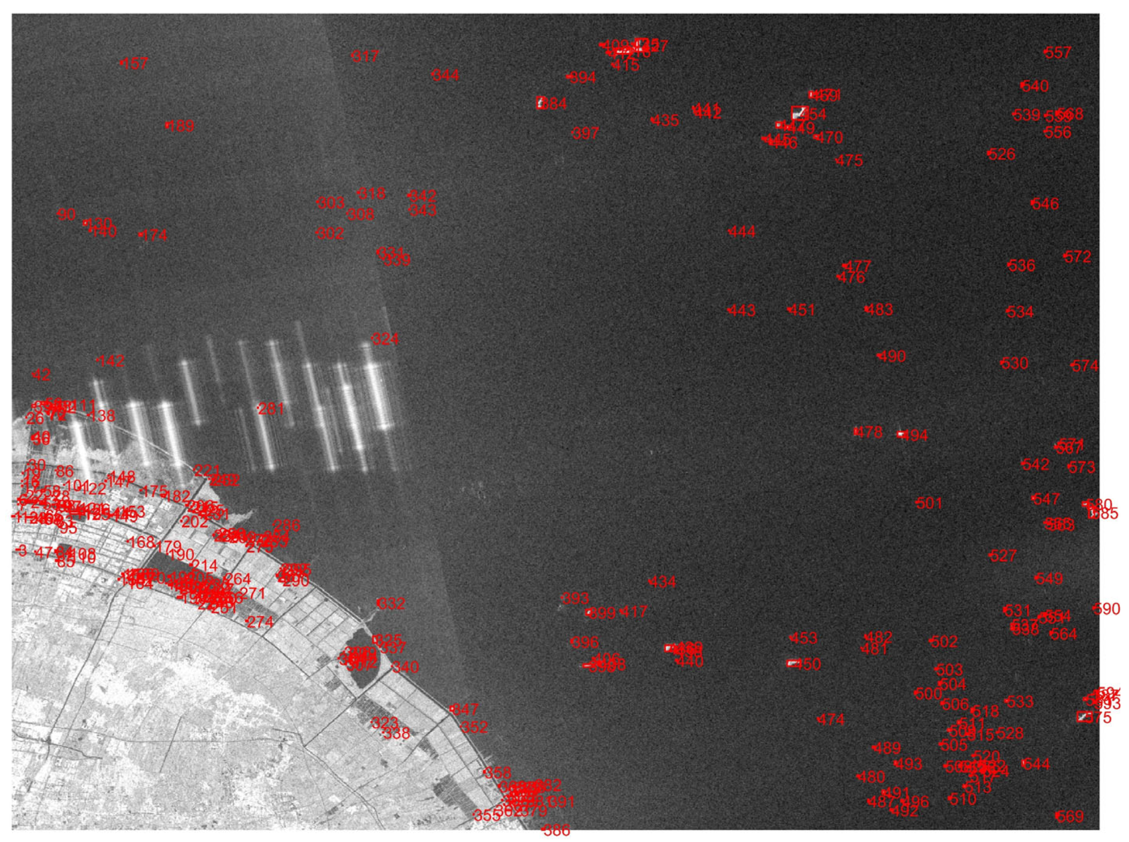
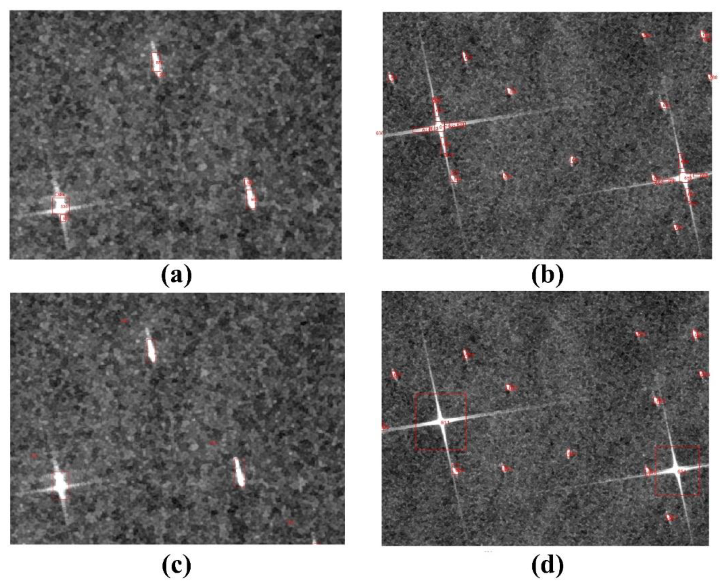
3.4. Candidate Detection

Two sub-images with 2855 × 2144 and 7833 × 5884 are clipped from Nos.1 and 2 to verify the accuracy of our method. Figure 6 and Figure 7 are intensity images in VH that the areas located in the nearshore area of the Qiongzhou Strait and the East China Sea area, respectively. The background of the Qiongzhou Strait area is relatively simple with land, island, and ships. However, the background of the East China Sea area is complex with land, radio-frequency interference (RFI) [33], ships, islands, and reefs [19,20], as well as the noise effects in VH polarization [34]. CFAR, Ostu, spectral residual, and corner detection are often used to obtain candidate detection results. However, the method is ineffective in cases where the variance between the object and the background is very varied. The method in [20] is used in the current work to obtain candidate targets for reducing the additional calculations and ensuring the candidate targets to be obtained is sufficient. However, there weresome invalid candidate targets due to some strong scattering or ship-like structures. Figure 8 and Figure 9 show the results of candidate detection of two sub-images, including the ships and false alarms caused by land targets, islands, and reefs. A total of 322 candidate targets containing ships and false alarms were obtained by pre-progress candidate detection, as in Figure 8 and Figure 9, respectively. A total of 18 true ships in the Qiongzhou Strait area and 79 true ships in the East China Sea area were obtained by Google Earth and SAR image interpretation.

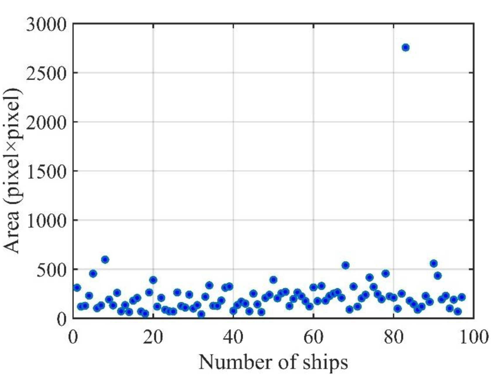
3.5. Boundary Box Optimization

Candidate targets on the binary map can be discontinuous due to the effect of speckles noise and sidelobe interference. Therefore, the bounding box of candidate targets may be inaccurate, as shown in Figure 10. Figure 10a,b show the bounding box of candidate targets without optimization. Further processing steps are applied to improve the boundary box of candidate target quality. A first quality improvement resides in the candidate target caused by sidelobe interference [35,36]. For the strongly scattering target, the presence of weak scattering features around strong scatterers due to sidelobe interference. The severe sidelobe of a strong scattering target is quite high and in many cases can be mistaken for a ship [35]. Hence, when an eight-connected or four-connected method is used to identify the target region of interest and obtain the bounding box of candidate targets, multiple bounding boxes will be generated for the same strongly scattering target. If the amplitude of one target is significantly higher than that of another, then the low boundary box of a weak scattering target close to a strong scattering target should be suppressed by the high sidelobe of the strong scattering target. The bounding boxes should be optimized to reduce the number of bounding boxes caused by sidelobe interference for the same candidate target and obtain accurate bounding boxes. Figure 11 shows the eight situations of bounding boxes. The red bounding box coordinates are $\mathrm{X}{1}_{top\_left}$, $\mathrm{Y}{1}_{top\_left}$, $\mathrm{X}{1}_{bottom\_right}$ and $\mathrm{Y}{1}_{bottom\_right}$, and the other irrelevant bounding boxes are typed in green and blue color with ${\mathrm{X}2}_{top\_left}$, ${\mathrm{Y}2}_{top\_left}$, ${\mathrm{X}2}_{bottom\_right}$ and ${\mathrm{Y}2}_{bottom\_right}$. The distance rule is introduced to reduce the irrelevant bounding boxes. The distance rule is defined in

Table 3. Rule of box merging.

Index	Position	Distance
1	Top	${\mathrm{Y}2}_{left}-{\mathrm{Y}1}_{right}$
2	Bottom	${\mathrm{Y}1}_{left}-{\mathrm{Y}2}_{right}$
3	Left	$\mathrm{X}{1}_{left}-\mathrm{X}{2}_{right}$
4	Right	$\mathrm{X}{2}_{left}-\mathrm{X}{1}_{right}$
5	Top and Left	$sqrt\left({\left({\mathrm{X}1}_{left}-{\mathrm{Y}1}_{right}\right)}^{\wedge }2+{\left({\mathrm{X}2}_{right}-{\mathrm{Y}2}_{left}\right)}^{\wedge }2\right)$
6	Top and Right	$sqrt\left({\left({\mathrm{X}1}_{right}-{\mathrm{Y}1}_{right}\right)}^{\wedge }2+{\left({\mathrm{X}2}_{left}-{\mathrm{Y}2}_{left}\right)}^{\wedge }2\right)$
7	Bottom and Left	$sqrt\left({\left({\mathrm{X}1}_{left}-{\mathrm{Y}1}_{left}\right)}^{\wedge }2+{\left({\mathrm{X}2}_{right}-{\mathrm{Y}2}_{right}\right)}^{\wedge }2\right)$
8	Bottom and Right	$sqrt\left({\left({\mathrm{X}1}_{right}-{\mathrm{Y}1}_{left}\right)}^{\wedge }2+{\left({\mathrm{X}2}_{left}-{\mathrm{Y}2}_{right}\right)}^{\wedge }2\right)$

. If the distance rule is less than 12, the bounding boxes are merged and updated by Equations (6)–(9). Figure 10c,d show the optimization result of the candidate targets bounding box. After the optimization, the position of the candidate targets bounding boxes is more accurate and reasonable. A second quality improvement resides in candidate targets caused by noise. The area and length of the bounding box from the candidate target are used to reduce the invalid candidate targets. Candidate target areas with less than 10 pixels, as well as side lengths greater than 180 pixels, are also considered noise and false alarms and are subsequently removed.

$${\mathrm{Xnew}}_{top\_left}=\min \left(\mathrm{X}{1}_{top\_left},\mathrm{X}{2}_{top\_left}\right)$$

(6)

$${\mathrm{Ynew}}_{top\_left}=\min \left(Y{1}_{top\_left},Y{2}_{top\_left}\right)$$

(7)

$${\mathrm{Xnew}}_{bottom\_right}=\max \left(\mathrm{X}{1}_{bottom\_right},\mathrm{X}{2}_{bottom\_right}\right)$$

(8)

$${\mathrm{Ynew}}_{bottom\_right}=\max \left(Y{1}_{bottom\_right},Y{2}_{bottom\_right}\right)$$

(9)

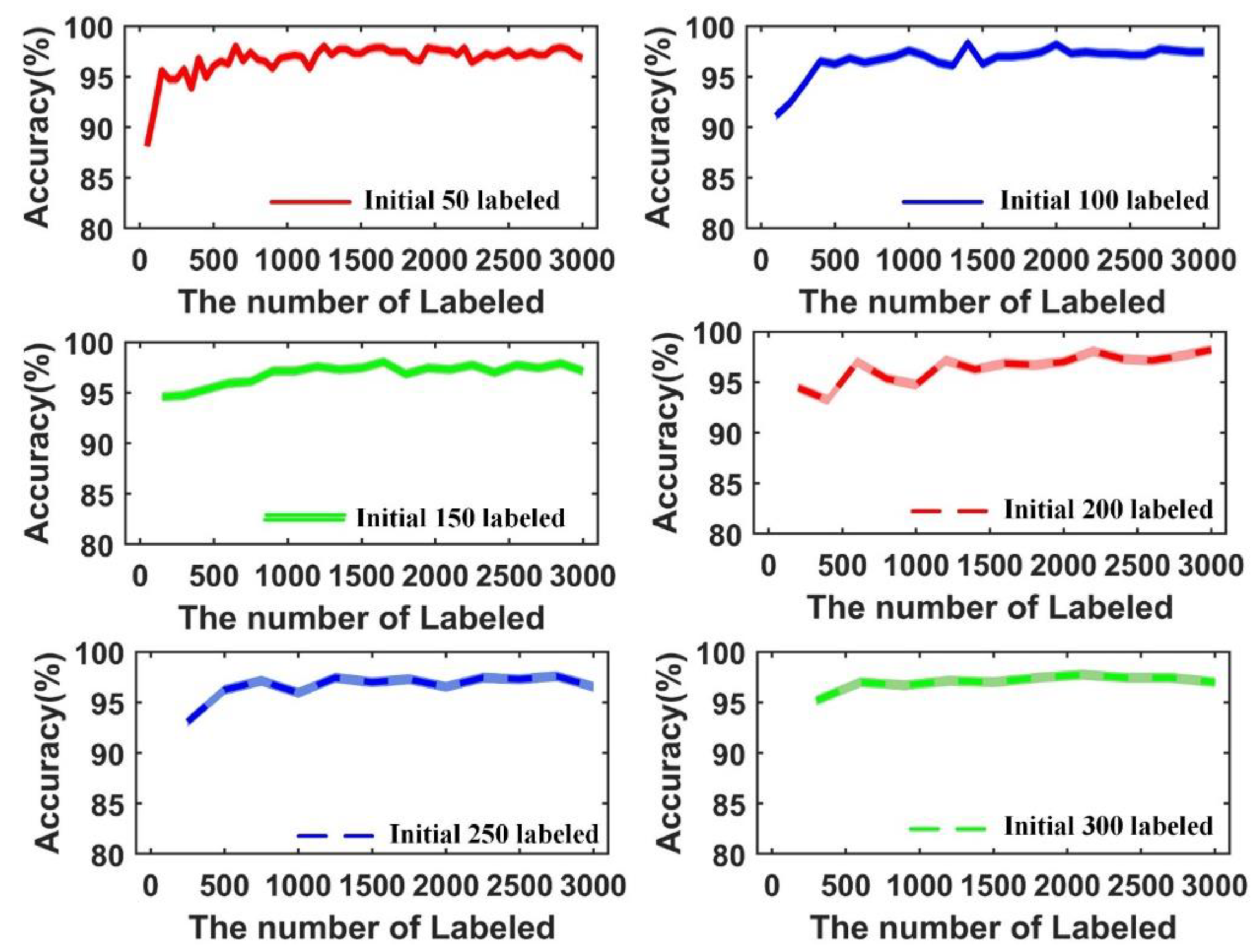
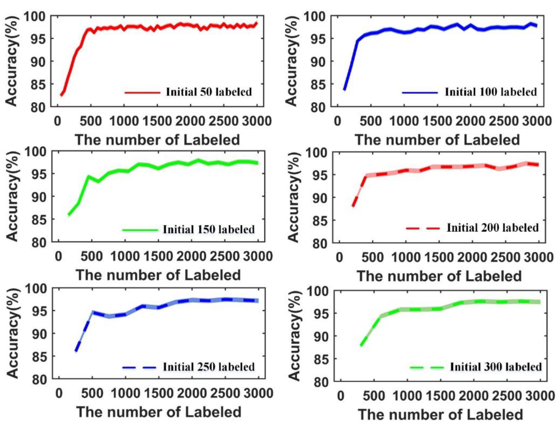
3.6. Effect of the Size of the Initial Labeled Training Set

In this experiment, we randomly select 3000 unlabeled slices from the dataset to form a training set $U_N$. The other slices are labeled and form the validation set. The test set comes from the other SAR image. We initialized a labeled dataset $L_k^0\left(k=50,100,150,200,250,300\right)$ with different sizes in the training stage to analyze the effect of the size of the labeled set on the detection results. The labeled training set size of 50 is taken as an example, and 50 slices are chosen from the 3000 unlabeled slices, and then inputted into the proposed learning model. Each of the 50 slices is labeled with the class with the maximum probability. A newly labeled slice is added to the labeled dataset, and the labeled set is trained once again until all the unlabeled slices are labeled. The same process is conducted for the labeled sets of other sizes. Figure 12 and Figure 13 show the change in the training accuracy with the initialed number of labeled slices by M-LeNet and ResNet18 with embedded active learning.

The accuracy of the training in the initial stage for M-LeNet with embedded active learning is higher when the number of the initially labeled training samples is larger. In addition, the profiles show that the initial training accuracy increases rapidly with the size of the labeled training set, and it reaches 95% when the labeled size is larger than 500 except the initially labeled 250 in Figure 12. The accuracy tends to convergence when the size of the training set is higher than 1500. A similar phenomenon is shown in Figure 13, and the accuracy of the training in the initial stage for ResNet18 with embedded active learning is higher when the number of the initial labeled training samples is increased. The difference is that the ResNet18 shows better performance than M-LeNet. ResNet network architecture was proposed by He et al. [30], and it achieved the best performance in ILSVRC 2015 classification task. In the initially labeled 50 training samples, the accuracy of ResNet18 is close to 90% at the first stage. The accuracy and convergence speed improve fast with increasing training samples, compared with M-LeNet with embedded active learning. The outstanding performance also illustrates that the ResNet architecture is suitable for ship detection. In

Table 4. The accuracy and time consumption of the proposed model with different sizes of initially labeled training sets.

Strategy	Method	Initial Labeled Training Set Size	Min Accuracy (%)	Max Accuracy (%)	Average Accuracy (%)	Time
Active-learning	Improved M-LeNet	50	82.41	98.50	96.36	2.32 h
		100	83.61	98.19	96.27	1.17 h
		150	85.86	97.90	95.56	47 min
		200	87.96	97.44	95.75	36 min
		250	86.01	97.44	95.26	29 min
		300	87.97	97.44	95.70	26 min
	Improved ResNet18	50	96.54	98.50	96.04	2.87 h
		100	93.38	98.50	97.37	1.46 h
		150	96.69	98.65	97.81	59 min
		200	96.39	98.20	97.77	45 min
		250	97.14	98.50	97.79	36 min
		300	94.44	97.94	97.75	31 min
Surpervised	M-LeNet	2932	90.44	97.97	97.08	1.18 h
	ResNet18		92.90	99.13	98.67	2.13 h
	RF		-	-	95.27	-
	SVM		-	-	94.54	-
	CNN [19]		-	-	97.20	-

, the training time and accuracy with different sizes of initially labeled training sets are listed. In the iterative training process of M-LeNet and ResNet18 with active learning, the accuracy for each iterative is recorded, and the minimum and maximum accuracy, average accuracy, and running time are counted for all the iterations. Meanwhile, the supervised learning strategy, with a large number of the labeled dataset of 2932 manually labeled training samples and 733 test samples, was used to train the M-LeNet, ResNet18, RF, SVM, and CNN methods. During the testing stage, the minimum and maximum accuracy, average accuracy, and running time are calculated. Table 4 also shows that the training time is highly correlated with the initially labeled set size. The model training time is shorter when the initially labeled set is larger. The maximum and the average accuracy rates exceed 98% and 97%, respectively, in all the experiments with different sizes of initial training labeled set.

Data-driven M-LeNet and ResNet18 in the supervised learning mechanisms, as well as SVM and RF in the machine learning mechanisms, are also used for evaluation. In those methods, the ratio of initial training and test sample is 8:2. The highest and the average accuracy rates of ResNet18 exceed 99% and 97%, which is better than that of ResNet with embedded active learning mechanisms. The highest accuracy and the average accuracy of M-LeNet exceed 98% and 97%, which are better than those of M-LeNet with embedded active learning mechanisms. The RF and SVM show poor accuracy with 95%, which is less than that of the CNN model. Similar performances from RF, SVM, and CNN are also shown in [19].

In the active learning mechanism, the accuracy gradually becomes better and rapidly converges with increasing numbers of labeled samples. However, the accuracy oscillation is relatively large compared with those of other models in the M-LeNet with embedded active learning mechanisms when the number of samples initially labeled is set as 150 and 250. When the data-driven CNN is applied to classification and recognition tasks, the steps are to train the model with a great number of labeled samples, obtain feedback from the model, and then adjust the parameters, continue to label the data, or modify the model architecture according to its performance until it meets the requirements. However, active learning is to train the model during the data labeling process. Thus, the quality of the data strongly influences the model. Under the condition of initially labeled 150 and 250 training samples in M-LeNet with active learning mechanism, or initially labeled 200 and 250 training samples in ResNet18 with active learning mechanism, the accuracy increases to a certain point and then suddenly decreases, and finally the accuracy increases and converges again during the iterative process. The reason for the decrease in accuracy is that the ships and false alarms are not completely and effectively distinguished, and there are samples which are difficult to separate, resulting in labeling errors. Thus, compared with convergence when the initial label sample size settings of 50 and 100, when the number of initially labeled samples is a set of 150 and 250, performance is slow due to the quality of data for each batch. However, as the number of samples increases, the learning ability of the model becomes strong and the accuracy increases and tends to be stable. The model architecture also influences the performance of active learning. The ResNet18 shows better performance than M-LeNet with embedded active learning, and this performance illustrates the effect of the model architecture. Moreover, the performance of M-LeNet and ResNet18 by active-learning strategy can be comparable to that of supervised training strategy when achieving 1000 epochs. However, the training time is greatly reduced.

3.7. Comparison of the Results Derived by Different Methods

We also compared the results achieved by SVM, RF, M-LeNet, and ResNet18 to demonstrate the efficiency of the improved lightweight M-LeNet and ResNet18 with embedded active learning scheme. The ratio of training samples and test samples is 8:2 in the supervised learning scheme, with 2932 manually labeled training samples and 733 test samples. In the active learning scheme, the manually initially labeled sample is set to 50, 100, 150, 200, 250, and 300. In the improved lightweight M-LeNet with embedded active learning schemes, manually labeled training samples of 50, 100, 150, 200, 250, and 300 are called M-LeNet-50, M-LeNet-100, M-LeNet-150, M-LeNet-200, M-LeNet-250, and M-LeNet-300, respectively. In the improved lightweight ResNet18 with embedded active learning schemes, manually labeled training sample of 50, 100, 150, 200, 250, and 300 are called ResNet-50, ResNet-100, ResNet-150, ResNet-200, ResNet-250, and ResNet-300, respectively. Two sub-images of the East China Sea area and the Qiongzhou Strait area with the sizes of 7833 × 5884 and 2855 × 2144, respectively are cropped to test the aforementioned methods. The backgrounds of the two sub-images for testing are complex and contain different scale-level ships. Figure 8 and Figure 9 show the candidate detection result of two sub-images, respectively. A total of 322 candidate targets containing ships and false alarms are obtained by pre-progress in Figure 8 and Figure 9. A total of 18 true ships in the Qiongzhou Strait area and 79 true ships in the East China Sea area are obtained by Google Earth and SAR image interpretation. Figure 14 shows the area of ships that can be obtained by the LabelImg annotation tool [37]. In those ships, the minimum size of the ship is 6 × 7 pixels, and most of the ships are less than 32 × 32 pixels. The targets with an area less than 32 × 32 are classified as small objects in the MS COCO nature dataset [38]. Most of the small-sized ships are nonmetallic fishing boats, so it is difficult to generate a strong scattering echo due to their simple structure, material, and target wobble [21]. The small-sized ships tend to be operated in the morning (02:00–11:00) and seem to be operated near shore [39]. Thus, most of the ships are most likely fishing boats; the size of the ships looks small and the scattering intensity also looks weak in the two SAR images acquired at 09:53 and 10:48 in the morning.

The Qiongzhou Strait area located in the nearshore is relatively simple. The quantitative assessment performance is listed in

Table 5. Quantitative assessment results in the Qiongzhou Strait.

Strategy	Method	Accuracy	Recall	Precision	F1-Score	Missed	False	Detected
Active-learn	M-LeNet-50	100%	1.0	1.0	1.0	0	0	18
	M-LeNet-100	100%	1.0	1.0	1.0	0	0	18
	M-LeNet-150	99.08	0.94	0.94	0.94	1	0	17
	M-LeNet-200	98.16	0.78	1.0	0.88	4	0	14
	M-LeNet-250	99.08	0.94	0.94	0.94	1	0	17
	M-LeNet-300	99.08	0.94	0.94	0.94	1	0	17
	ResNet-50	100%	1.0	1.0	1.0	0	0	18
	ResNet-100	100%	1.0	1.0	1.0	0	0	18
	ResNet-150	98.62	1.0	0.86	0.92	0	3	18
	ResNet-200	99.54	1.0	0.95	0.97	0	0	18
	ResNet-250	100%	1.0	1.0	1.0	0	0	18
	ResNet-300	100%	1.0	1.0	1.0	0	0	18
Surpervised	M-LeNet	99.54	1.0	0.95	0.97	0	1	18
	ResNet18	100%	1.0	1.0	1.0	0	0	18
	SVM	99.54	1.0	0.95	0.97	0	1	18
	RF	100%	1.0	1.0	1.0	0	0	18

. The best accuracy in the training stage is used to evaluate for M-LeNet and ResNet18 by the active learning strategy. The detection results show that the highest recall, accuracy, and F1-score of 1.0, 100%, and 1.0, respectively is achieved by the M-LeNet-50, M-LeNet-100, ResNet18-50, ResNet18-100, ResNet18-250, and ResNet18-300. In the supervised learning strategy, the ResNet18 and RF can achieve a recall of 1.0, an accuracy of 100%, and an F1-score of 1.0. The performance of M-LeNet-150, M-LeNet-200, and M-LeNet-250 is not as good as the supervised learning strategy of M-LeNet, ResNet18, SVM, and RF. Figure 15 shows that the best detection results are achieved by active learning and supervised strategy.

The East China sea area located on the nearshore is relatively complex. The RFI could be observed in the left of Figure 7, which has similar intensity to ships and can degrade ocean interpretation [33]. A new method was once proposed to discriminate ships from RFIs based on non-circularity and non-gaussianity [32]. However, the candidate detection results show that the preprocessing reduces the effect of RFI, as shown in Figure 9.

Table 6. Quantitative assessment results in the East China Sea.

Strategy	Method	Accuracy	Recall	Precision	F1-Score	Missed	False	Detected
Active-learn	M-LeNet-50	97.78	0.92	1.0	0.96	6	0	73
	M-LeNet-100	97.41	0.92	0.99	0.95	6	1	72
	M-LeNet-150	97.78	0.92	1.0	0.96	6	0	73
	M-LeNet-200	95.93	0.89	0.97	0.93	9	2	70
	M-LeNet-250	97.04	0.90	1.0	0.95	8	0	71
	M-LeNet-300	97.04	0.92	0.97	0.95	6	2	73
	ResNet-50	97.41	0.95	0.96	0.96	4	3	75
	ResNet-100	97.04	0.92	0.97	0.95	6	2	73
	ResNet-150	95.19	0.90	0.93	0.92	8	5	71
	ResNet-200	96.30	0.92	0.95	0.94	6	4	73
	ResNet-250	96.30	0.90	0.97	0.93	8	2	71
	ResNet-300	97.04	0.92	0.97	0.95	6	2	73
Surpervised	M-LeNet	96.67	0.91	0.97	0.94	7	2	72
	ResNet18	97.04	0.92	0.97	0.95	6	2	73
	SVM	90.74	0.95	0.78	0.86	4	21	75
	RF	89.63	0.82	0.82	0.82	14	14	65

shows the quantitative evaluation results by active learning and supervised learning strategy. The result shows that the highest accuracy and F1-score of 97.78% and 0.96 is achieved by the M-LeNet-50 and M-LeNet-150. The highest accuracy and F1-score of 97.41% and 0.96 is achieved by the ResNet-50. The performance of M-LeNet and ResNet18 with the supervised learning strategy can achieve the best performance with the accuracy and F1-score better than 96% and 0.94, but the RF and SVM have the worst result. Figure 16 shows the best detection results by the active learning and supervised strategy. In the CNN detector field, an area smaller than 32 × 32 is defined as small objects, and most ships in the test data are much less than 32 × 32 pixels. The result shows that 73 true ships are detected, six true ships are undetected, and zero false alarm is misclassified as the ship. The reason is that the ship’s RCS is weak, and some ships have similar backscattering with the ocean [21]. The results of RF and SVM show that some false alarms are misclassified as ships due to similar characteristics with islands and reefs.

4. Discussion

In this article, we mainly discuss ship detection for CNN-based VH polarization. As an alternative to end-to-end CNN-based detectors [8,9,40,41,42,43], we proposed a two-stage ship detection method. Although similar ship detection methods were proposed by [19,20,44], a large number of samples needed to be labeled and prepared before the CNN began to train. A ship detection method was proposed based on an improved lightweight M-LeNet and ResNet18 deep learning network with an active learning strategy to enable suitability of the CNN model for detecting small ships with a small amount of labeled sample data, as well as reduce labor cost. In the CNN-based active learning strategies, the initially labeled sample size only affects the initial accuracy and training time. The performance of the different numbers of labeled data is similar to those of [24]. As the unlabeled database is updated with the samples by active learning strategy, the accuracy of the model is gradually becoming higher and stabilized. He et al. [45] once emphasized that the convergence can be accelerated by using models that have been pre-trained on ImageNet in the early stage of training. It is not feasible that pretraining on ImageNet would require a significant amount of time and computational power [10]. Transfer training can converge with suitable time and small datasets, but data differences between SAR images and natural images are ignored [9]. By the application of a suitable active learning method and an adequate number of iterations, we can achieve satisfactory convergence. However, some existing ship-like structures produce similar characteristics to ships. In addition, the detection effectiveness of SAR ships is influenced by many factors, including polarimetry, image resolution, incidence angle, ocean dynamics parameters, ship size, and ship orientation [46]. In some active learning strategies, the model appears not very well converged. Thus, the poor detection result is obtained in the experiment. In the future, the sea state information should be further considered to obtain satisfactory convergence to improve ship detection. In addition, the small-sized ship is difficult to detect due to the weak target scattering and few pixels. In the next work, we will consider further optimization of the model to improve weak scattering target detection by combining polarization features and scattering features. In addition, ship detection in SAR images has become an important technology-based on CNNs, several SAR ship detection methods have been proposed by scholars using Radarsta-1/2, TerraSAR-X, Sentinel-1 A/B, GF-3 datasets [7,8,14]. However, they do not receive support from AIS information, nor Google Earth images, so the annotation process of their dataset relies heavily on the experience of experts, which likely leads to a decrease in the authenticity of the dataset [14,47]. In our experiment, the ships and false alarms are annotated by visual interpretation, expert knowledge, and Google Earth images; it is progress. Due to a lack of AIS information, it may be that there are wrong samples in the dataset. Hence, in the future, it will be necessary to obtain AIS information corresponding to SAR data to improve the performance of ship detection.

5. Conclusions

We mainly discuss ship detection for CNN-based VH polarization in this article. As an alternative to end-to-end CNN-based detectors, a new method was proposed for SAR image ship detection in the case of a small number of training samples. The main steps of the proposed method include candidate target detection, boundary box optimization and ship detection. Compared with the SVM, RF, M-LeNet, and ResNet18, which need a great number of labeled samples, the proposed ship detection method based on improved lightweight M-LeNet and ResNet18 network with an active learning strategy can label the training data automatically, and shows high reliability with only a small number of training samples. The experimental results also show that it performs well for small-sized ships nearshore with the proposed method. In the future, the way to use the polarimetric features and combine them with CNN to further improvements in the detection accuracy of the small-sized ship is worth investigating.

References

1. Lee, J.-S.; Pottier, E. Polarimetric Radar Imaging: From Basics to Applications; CRC Press: Boca Raton, FL, USA, 2009. [Google Scholar]
2. Geng, X.; Li, X.-M.; Velotto, D.; Chen, K.-S. Study of the polarimetric characteristics of mud flats in an intertidal zone using C-and X-band spaceborne SAR data. Remote. Sens. Environ. 2016, 176, 56–68. [Google Scholar] [CrossRef]
3. Ai, J.; Qi, X.; Yu, W.; Deng, Y.; Liu, F.; Shi, L. A New CFAR Ship Detection Algorithm Based on 2-D Joint Log-Normal Distribution in SAR Images. IEEE Geosci. Remote. Sens. Lett. 2010, 7, 806–810. [Google Scholar] [CrossRef]
4. An, W.; Xie, C.; Yuan, X. An Improved Iterative Censoring Scheme for CFAR Ship Detection With SAR Imagery. IEEE Trans. Geosci. Remote Sens. 2014, 52, 4585–4595. [Google Scholar] [CrossRef]
5. Leng, X.; Ji, K.; Yang, K.; Zou, H. A Bilateral CFAR Algorithm for Ship Detection in SAR Images. IEEE Geosci. Remote. Sens. Lett. 2015, 12, 1536–1540. [Google Scholar] [CrossRef]
6. Hazra, A.; Choudhary, P.; Sheetal Singh, M. Recent Advances in Deep Learning Techniques and Its Applications: An Overview. Adv. Biomed. Eng. Technol. 2021, 103–122. [Google Scholar]
7. Li, J.; Qu, C.; Shao, J. Ship detection in SAR images based on an improved faster R-CNN. In Proceedings of the 2017 SAR in Big Data Era: Models, Methods and Applications (BIGSARDATA), Beijing, China, 13–14 November 2017; pp. 1–6. [Google Scholar]
8. Wang, Y.; Wang, C.; Zhang, H.; Dong, Y.; Wei, S. A SAR dataset of ship detection for deep learning under complex backgrounds. Remote Sens. 2019, 11, 765. [Google Scholar] [CrossRef] [Green Version]
9. Wang, Y.; Wang, C.; Zhang, H.; Dong, Y.; Wei, S. Automatic Ship Detection Based on RetinaNet Using Multi-Resolution Gaofen-3 Imagery. Remote Sens. 2019, 11, 531. [Google Scholar] [CrossRef] [Green Version]
10. Chen, C.; He, C.; Hu, C.; Pei, H.; Jiao, L. A deep neural network based on an attention mechanism for SAR ship detection in multiscale and complex scenarios. IEEE Access 2019, 7, 104848–104863. [Google Scholar] [CrossRef]
11. Cui, Z.; Li, Q.; Cao, Z.; Liu, N. Dense attention pyramid networks for multi-scale ship detection in SAR images. IEEE Trans. Geosci. Remote Sens. 2019, 57, 8983–8997. [Google Scholar] [CrossRef]
12. Zhao, Y.; Zhao, L.; Xiong, B.; Kuang, G. Attention receptive pyramid network for ship detection in SAR images. IEEE J. Sel. Top. Appl. Earth Observ. 2020, 13, 2738–2756. [Google Scholar] [CrossRef]
13. Dai, W.; Mao, Y.; Yuan, R.; Liu, Y.; Pu, X.; Li, C. A Novel Detector Based on Convolution Neural Networks for Multiscale SAR Ship Detection in Complex Background. Sensors 2020, 20, 2547. [Google Scholar] [CrossRef] [PubMed]
14. Wei, S.; Zeng, X.; Qu, Q.; Wang, M.; Su, H.; Shi, J. HRSID: A high-resolution SAR images dataset for ship detection and instance segmentation. IEEE Access 2020, 8, 120234–120254. [Google Scholar] [CrossRef]
15. Chen, P.; Li, Y.; Zhou, H.; Liu, B.; Liu, P. Detection of Small Ship Objects Using Anchor Boxes Cluster and Feature Pyramid Network Model for SAR Imagery. J. Mar. Sci. Eng. 2020, 8, 112. [Google Scholar] [CrossRef] [Green Version]
16. Fu, J.; Sun, X.; Wang, Z.; Fu, K. An anchor-free method based on feature balancing and refinement network for multiscale ship detection in SAR images. IEEE Trans. Geosci. Remote. Sens. 2020, 59, 1331–1344. [Google Scholar] [CrossRef]
17. Zhang, G.; Li, Z.; Li, X.; Yin, C.; Shi, Z. A Novel Salient Feature Fusion Method for Ship Detection in Synthetic Aperture Radar Images. IEEE Access 2020, 8, 215904–215914. [Google Scholar] [CrossRef]
18. Xu, C.; Yin, C.; Wang, D.; Han, W. Fast ship detection combining visual saliency and a cascade CNN in SAR images. IET Radar Sonar Navig. 2020, 14, 1879–1887. [Google Scholar] [CrossRef]
19. Wang, Z.; Yang, T.; Zhang, H. Land contained sea area ship detection using spaceborne image. Pattern Recognit. Lett. 2020, 130, 125–131. [Google Scholar] [CrossRef]
20. Geng, X.; Shi, L.; Yang, J.; Li, P.; Zhao, L.; Sun, W.; Zhao, J. Ship Detection and Feature Visualization Analysis Based on Lightweight CNN in VH and VV Polarization Images. Remote Sens. 2021, 13, 1184. [Google Scholar] [CrossRef]
21. Liu, G.; Zhang, X.; Meng, J. A Small Ship Target Detection Method Based on Polarimetric SAR. Remote Sens. 2019, 11, 2938. [Google Scholar] [CrossRef] [Green Version]
22. Liu, A.K.; Peng, C.Y.; Weingartner, T.J. Ocean-ice interaction in the marginal ice zone. J. Geophys. Res. 1994, 99, 22391–22400. [Google Scholar] [CrossRef]
23. Villas Bôas, A.B.; Ardhuin, F.; Ayet, A.; Bourassa, M.A.; Brandt, P.; Chapron, B.; Cornuelle, B.D.; Farrar, J.T.; Fewings, M.R.; Fox-Kemper, B.; et al. Integrated Observations of Global Surface Winds, Currents, and Waves: Requirements and Challenges for the Next Decade. Front. Mar. Sci. 2019, 6, 425. [Google Scholar] [CrossRef]
24. Yoo, D.; Kweon, I.S. Learning loss for active learning. In Proceedings of the IEEE Conference on Computer Vision and Pattern Recognition, Long Beach, CA, USA, 15–20 June 2019; pp. 93–102. [Google Scholar]
25. Settles, B. Active Learning Literature Survey; University of Wisconsin: Madison, WI, USA, 2009. [Google Scholar]
26. Ren, P.; Xiao, Y.; Chang, X.; Huang, P.-Y.; Li, Z.; Chen, X.; Wang, X. A Survey of Deep Active Learning. arXiv 2019, arXiv:2009.00236. [Google Scholar]
27. Lewis, D.D.; Catlett, J. Heterogeneous uncertainty sampling for supervised learning. In Machine Learning Proceedings 1994; Elsevier: Amsterdam, The Netherlands, 1994; pp. 148–156. [Google Scholar]
28. Yang, L.; Zhang, Y.; Chen, J.; Zhang, S.; Chen, D.Z. Suggestive annotation: A deep active learning framework for biomedical image segmentation. In Proceedings of the International Conference on Medical Image Computing and Computer-Assisted Intervention, Quebec City, QC, Canada, 11–13 September 2017; pp. 399–407. [Google Scholar]
29. Vezhnevets, A.; Buhmann, J.M.; Ferrari, V. Active learning for semantic segmentation with expected change. In Proceedings of the 2012 IEEE conference on computer vision and pattern recognition, Providence, RI, USA, 16–21 June 2012; pp. 3162–3169. [Google Scholar]
30. Siddiqui, Y.; Valentin, J.; Nießner, M. Viewal: Active learning with viewpoint entropy for semantic segmentation. In Proceedings of the IEEE/CVF Conference on Computer Vision and Pattern Recognition, Seattle, WA, USA, 13–19 June 2020; pp. 9433–9443. [Google Scholar]
31. He, K.; Zhang, X.; Ren, S.; Sun, J. Deep residual learning for image recognition. In Proceedings of the IEEE Conference on Computer Vision and Pattern Recognition, Las Vegas, NV, USA, 27–30 June 2016; pp. 770–778. [Google Scholar]
32. Pelich, R.; Longépé, N.; Mercier, G.; Hajduch, G.; Garello, R. Performance evaluation of Sentinel-1 data in SAR ship detection. In Proceedings of the 2015 IEEE International Geoscience and Remote Sensing Symposium (IGARSS), Milan, Italy, 26–31 July 2015; pp. 2103–2106. [Google Scholar]
33. Leng, X.; Ji, K.; Zhou, S.; Xing, X.; Zou, H. Discriminating Ship From Radio Frequency Interference Based on Noncircularity and Non-Gaussianity in Sentinel-1 SAR Imagery. IEEE Trans. Geosci. Remote. Sens. 2018, 57, 352–363. [Google Scholar] [CrossRef]
34. Sun, Y.; Li, X.M. Denoising Sentinel-1 Extra-Wide Mode Cross-Polarization Images Over Sea Ice. IEEE Trans. Geosci. Remote. Sens. 2020, 59, 2116–2131. [Google Scholar] [CrossRef]
35. Zhu, X.; He, F.; Ye, F.; Dong, Z.; Wu, M. Sidelobe Suppression with Resolution Maintenance for SAR Images via Sparse Representation. Sensors 2018, 18, 1589. [Google Scholar] [CrossRef] [PubMed] [Green Version]
36. Stankwitz, H.C.; Dallaire, R.J.; Fienup, J.R. Nonlinear apodization for sidelobe control in SAR imagery. IEEE Trans. Aerosp. Electron. Syst. 1995, 31, 267–279. [Google Scholar] [CrossRef]
37. Tzutalin, D. LabelImg. GitHub Code. 2015. Available online: https://github.com/tzutalin/labelImg (accessed on 16 July 2021).
38. Lin, T.-Y.; Maire, M.; Belongie, S.; Hays, J.; Perona, P.; Ramanan, D.; Dollár, P.; Zitnick, C.L. Microsoft coco: Common objects in context. In Proceedings of the European Conference on Computer Vision-ECCV 2014, Zurich, Swizerland, 6–12 September 2014; pp. 740–755. [Google Scholar]
39. Snapir, B.; Waine, T.W.; Biermann, L. Maritime Vessel Classification to Monitor Fisheries with SAR: Demonstration in the North Sea. Remote Sens. 2019, 11, 353. [Google Scholar] [CrossRef] [Green Version]
40. Ma, M.; Chen, J.; Liu, W.; Yang, W. Ship Classification and Detection Based on CNN Using GF-3 SAR Images. Remote Sens. 2018, 10, 2043. [Google Scholar] [CrossRef] [Green Version]
41. Wang, Y.; Li, W.; Li, X.; Sun, X. Ship Detection by Modified RetinaNet. In Proceedings of the 2018 10th IAPR Workshop on Pattern Recognition in Remote Sensing (PRRS) 2018, Beijing, China, 19–20 August 2018; pp. 1–5. [Google Scholar]
42. Zhao, J.; Zhang, Z.; Yu, W.; Truong, T.-K. A Cascade Coupled Convolutional Neural Network Guided Visual Attention Method for Ship Detection From SAR Images. IEEE Access 2018, 6, 50693–50708. [Google Scholar] [CrossRef]
43. Chang, Y.-L.; Anagaw, A.; Chang, L.; Wang, Y.C.; Hsiao, C.-Y.; Lee, W.-H. Ship Detection Based on YOLOv2 for SAR Imagery. Remote Sens. 2019, 11, 786. [Google Scholar] [CrossRef] [Green Version]
44. Liu, Y.; Zhang, M.H.; Xu, P.; Guo, Z.W. SAR ship detection using sea-land segmentation-based convolutional neural network. In Proceedings of the 2017 International Workshop on Remote Sensing with Intelligent Processing (RSIP), Shanghai, China, 18–21 May 2017; pp. 1–4. [Google Scholar]
45. He, K.; Girshick, R.; Dollar, P. Rethinking ImageNet Pre-Training. In Proceedings of the 2019 IEEE/CVF International Conference on Computer Vision (ICCV), Seoul, Korea, 27 October–2 November 2019; pp. 4917–4926. [Google Scholar]
46. Tings, B.; Bentes, C.; Velotto, D.; Voinov, S. Modelling ship detectability depending on TerraSAR-X-derived metocean parameters. CEAS Space J. 2019, 11, 81–94. [Google Scholar] [CrossRef] [Green Version]
47. Zhang, T.; Zhang, X.; Ke, X.; Zhan, X.; Shi, J.; Wei, S.; Pan, D.; Li, J.; Su, H.; Zhou, Y.; et al. LS-SSDD-v1.0: A Deep Learning Dataset Dedicated to Small Ship Detection from Large-Scale Sentinel-1 SAR Images. Remote Sens. 2020, 12, 2997. [Google Scholar] [CrossRef]
Figure 1. Deep active learning flowchart.
Remotesensing 13 03400 g001
Figure 2. Improved ResNet18 baseline backbone and loss prediction module.
Remotesensing 13 03400 g002
Figure 3. Improved M-LeNet baseline backbone and loss prediction module.
Remotesensing 13 03400 g003
Figure 4. Candidate slices of (a) false alarms, and (b) ships.
Remotesensing 13 03400 g004
Figure 5. Candidate false alarms and their corresponding images in Google Earth.
Remotesensing 13 03400 g005
Figure 6. Sub-image of VH polarization in the Qiongzhou Strait area.
Remotesensing 13 03400 g006
Figure 7. Sub-image of VH polarization in the East China Sea area.
Remotesensing 13 03400 g007
Figure 8. The candidate detection result of the VH polarization sub-image in the Qiongzhou Strait area.
Remotesensing 13 03400 g008
Figure 9. The candidate detection result of the VH polarization sub-image in the East China Sea area.
Remotesensing 13 03400 g009
Figure 10. Results of bounding box optimization. (a,b) are the bounding box of candidate targets without optimization; (c,d) are the bounding box of candidate targets with optimization.
Remotesensing 13 03400 g010
Figure 11. Position of bounding boxes (red box: the main box, blue and green boxes: the box caused by sidelobe interference that needs to be merged).
Remotesensing 13 03400 g011
Figure 12. Change in the initial training accuracy with the number of labeled slices by improved M-LeNet with active learning.
Remotesensing 13 03400 g012
Figure 13. Change in the initial training accuracy with the number of labeled slices by improved ResNet18 with active learning.
Remotesensing 13 03400 g013
Figure 14. Areas of ships.
Remotesensing 13 03400 g014
Figure 15. Results of the different methods in the Qiongzhou Strait. ((a): SVM, (b): RF, (c): Supervised-learning M-LeNet, (d): Supervised-learning ResNet18, (e): Active learning M-LeNet, and (f): Active learning ResNet18). Red rectangle: ship; green rectangle: missed ship; and blue rectangle: false alarm.
Remotesensing 13 03400 g015
Figure 16. Result of the different methods in the East China Sea. ((a): SVM, (b): RF, (c): Supervised-learning M-LeNet, (d): Supervised-learning ResNet18, (e): Active learning M-LeNet, and (f): Active learning ResNet18). Red rectangle: ship; green rectangle: miss-detection; and blue rectangle: false alarm.
Remotesensing 13 03400 g016