Abstract
The creation and protection of surfing breaks along populated coastlines have become a consideration for many councils and governments as surfing breaks are a major driver of tourism. To assess the surf amenity of surfing breaks, a quantitative and objective assessment method is required. A new wave peel tracking (WPT) method has been developed using a shore-based camera to assess surf amenity by measuring and quantifying potential surfing ride rate, length, duration, speed and direction on a wave-by-wave basis. The wave peel (or “curl” below the wave peak) is the optimal surfing region on a wave, and each wave peel track represents a surfable ride. Wave peel regions are identified, classified and tracked using traditional and machine learning-based computer vision techniques. The methodology is validated by comparing the rectified wave peel tracks with GPS-measured tracks from surfers in the wave peel regions. The WPT methodology is evaluated with data from a reef and adjacent natural beach at the Gold Coast, Australia. The reef produced longer ride lengths than the nearshore region and showed a consistent breaking location along the reef crest. Spatial maps of the wave peel tracks show the influence of tides on the wave breaking patterns and intensity. The WPT algorithm provides a robust, automated method for quantifying surf amenity to provide baseline data for surf break conservation. The methodology has potential uses to verify numerical modelling of surf breaks and to assess the impact of coastal development on surf breaks.
1. Introduction
Millions of people worldwide choose to reside near or visit beaches to enjoy surfable waves. Coastal populations are increasing each year and infrastructure is being constructed closer to the beach or within the nearshore zone itself. Increased nearshore development coupled with rising sea levels has led to infrastructure and buildings at risk to erosion from large storm events. This has prompted responses from local councils to develop beach management strategies which can involve large-scale works such as sand replenishment and building of coastal structures. These works can maintain or improve surf amenity with careful design but can also diminish surf amenity. In the effort to assess surf amenity, one of the main challenges is quantitative and objective assessment. This paper presents a novel automated wave peel tracking (WPT) technique to quantitatively and objectively assess surf amenity using a shore-based camera.
Surf amenity has been under threat from coastal developments and natural processes in a number of famed surf breaks around the world. One such example is a point break in Bali which was “destroyed” due to a seawall constructed to protect a new high rise [1]. Another famous example of a complex surf amenity issue was the effect of the Tweed River training walls on the Coolangatta beaches (Gold Coast, Australia). Longshore sediment transport was interrupted, leading to diminished surf amenity at the previously world-renowned Kirra point break. A carefully designed sand transfer system has since been implemented, which has restored and improved surf amenity to most of the Coolangatta point breaks. This highlights the importance of considering surf amenity in coastal management [2]. Many other surfing breaks face the threat of degradation [3]. The World Surfing Reserve was established to ensure that world class surfing destinations (including the Coolangatta point breaks) are protected in the future [4]. A challenge moving forward is to continue to protect the coastlines from erosion and accommodate growing populations while preserving or creating surf amenity. To achieve this, surf breaks need to be better understood using a quantitative approach that allows objective comparison between other surf breaks and validation of numerical modelling for surf breaks.
While surf amenity can be assessed qualitatively by community response from surfers, quantitative assessment is much more insightful and objective. There have been several attempts to quantitively assess surf amenity using visual observations, numerical modelling and remote sensing approaches. From visual observations, the ‘peel angle’ can be extracted by finding the angle between the breakpoint position direction and the wave crest [5]. The peel angle is considered one of the most important surf amenity parameters [6] and has previously been effectively extracted manually from observations of the surf zone from images [7,8,9]. Other important parameters such as the ‘section length’ have been manually analysed from rectified images of the surf zone [10]. Numerical models have been used in New Zealand to define wave breaking envelopes at a surf break and assess how they are affected by morphological change [11]. Numerical modelling has also been used at the Gold Coast, Australia, for providing insight into surf amenity with an approach similar to WPT [12]. Numerical modelling is critical for the future design of effective surfing infrastructure, but requires comprehensive field data for validation, which is presently lacking.
Remote sensing techniques are commonly used for assessment of coastal environments and for validation of numerical models. Video timestacks have been used for many years in coastal research [13] to measure or track breaking waves and wave runup [14,15,16,17]. Recent methods have involved the use of convolutional neural networks (CNN), for classifying beach states, wave breaker types and estimating wave height and wave period [18,19,20,21]. Wave crest tracking has been achieved through using a ‘Mixture of Gaussians’ approach and a spatial transformer network [22,23]. These remote sensing applications in coastal research show the effectiveness of using computer vision techniques to extract wave related data, particularly those involving machine learning. However, none of these applications can directly assess surf amenity.
To the authors’ knowledge, the only prior automated and quantitative approaches to assess surf amenity through remote sensing include identification of length and orientation of surfable sandbars, analysis of cumulative wave breaking regions, tracking of bores and the direct tracking of surfers [24,25,26,27]. Identification of length and orientation of surfable sandbars and analysis of heat maps of cumulative wave breaking provide good spatial information over a whole surf break, but neither method gives detailed wave-by-wave insight at the precision of individual wave peel regions. Tracking bores allows wave-by-wave insights but cannot provide precise, individual wave peel region data. Tracking surfers provides unique insight into a surfer’s assessment of surfed wave peel regions; however, this method cannot assess surf amenity where there are no surfers and is subject to the ability of the surfer, their style of surfing and crowding of the surf break. The WPT approach solves these issues by tracking the surfable wave peel regions on a wave-by-wave basis. The WPT methodology developed here has been fully tested and verified at a surfable reef and adjacent nearshore region, using video recordings and GPS surfer tracks obtained on the 13th January 2021 from a shore-based CCTV camera on a 12-storey building. WPT data were extracted, rectified and processed to quantify surfing metrics, including average ride duration, average ride length, average ride speed and ride rate, together with spatial maps of the WPTs and ride direction distributions. The WPT results also provide a unique way to analyse wave breaking activity in natural surf zones and has the potential to be used to verify or calibrate numerical models for surf break design.
The aim of this paper is to detail the WPT methodology and evaluate it through assessing surf amenity over a reef and nearshore region. This paper is organised as follows: Section 2 presents the WPT methodology, including the definition of the wave peel region and description of the applied computer vision and machine learning techniques. A comprehensive description of the field site and the data collected is given in Section 3. Quantitative results comparing derived surf metrics on the reef and adjacent surf zone are presented in Section 4, together with comparisons from direct GPS tracking of surfers. Section 5 provides a discussion of the WPT results, applications of the methodology and future research directions.
2. Methods
The quality of surf has long been informally assessed by surfers through visual observation of the peeling edge of a breaking wave, referred to in this work as a wave peel region. An important feature of quality surf is the presence of surfable, long-duration peeling waves, moving either left or right from a consistent location. Sand bars and hard structure point breaks often shape waves with such desirable wave peel regions. When a surfer is visually assessing the surf conditions, they are effectively ‘wave peel tracking’ to evaluate the potential ride length, ride duration, ride speed and the rate at which they can catch rides. This assessment approach has been used to similar effect manually by Scarfe [9], to trace ‘breaking wave paths’ at key surfing sections for extracting peel angles and peel rates. The work in this paper builds on that approach through the WPT algorithm by providing a more detailed surf amenity assessment automatically at very high temporal and spatial resolution. This is achieved by combining machine learning with traditional computer vision methods, including background subtraction, blob detection, object tracking, convolution neural networks (CNNs) and homography. The required input is a video of the surf zone to be evaluated and the output is a list of geo-rectified WPTs. A wide range of metrics can then be derived from the WPTs, including average ride duration, average ride length, maximum ride length, average ride speed, ride rate and ride direction. This section details the WPT algorithm, broken up into the following subsections: definition of the wave peel region, motion detection, wave peel region classification, wave peel tracking, rectification and post processing. A video of the WPT process is available to watch, which provides a visual representation of what is described in the following sections (https://youtu.be/vZj_1pZiaI4, accessed on 18 August 2021). All processed videos in this work are available through the YouTube playlist link in the Supplementary Materials of this paper.
2.1. Definition of the Wave Peel Region
The wave peel region is defined for this work as illustrated in Figure 1 a,b, with the u,v coordinates of the centre of the wave peel region being tracked. This is adapted from the conventional definition of the position of the ‘peel’ used for working out peel angles [5]. The vertical centre (full yellow line) is defined as the intersection of the mean water level with the wave face. This position has been estimated to be either 1/5 or 1/3 of the wave face height [15,28]. The choice of either of these does not matter significantly for rectification given the field of view and the resolution of video generally used; however, a value of 1/5 has been chosen. The horizontal centre (full blue line) is defined to be halfway between the leading edge of whitewater (the lip of the wave) and the start of fully developed whitewater. This definition of the wave peel region is appropriate for both plunging and spilling type waves and is used in the verification process of the WPT software in Section 4.1.
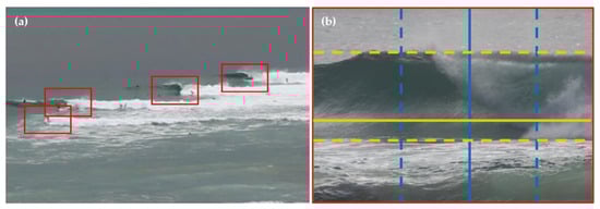
Figure 1.
(a) Manually annotated wave peel regions at Snapper Rocks, QLD, Australia. (b) Precise definition of the wave peel centre for WPT purposes. The vertical centre is defined by the yellow lines; the horizontal centre is defined by the blue lines (photo from Currumbin Beach QLD, Australia).
2.2. Motion Detection
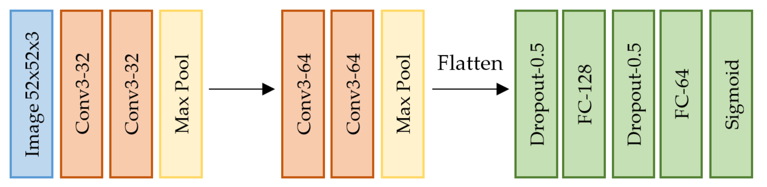
Wave crests move with relatively constant celerity towards the shoreline (decelerating very slowly). As they break, wave peel regions propagate laterally along the wave crests. With the appropriate viewing angle, wave peel regions move approximately horizontally in the camera image. Therefore, background subtraction can be used as the first step to identify the wave peel regions in a video sequence. Background subtraction involves taking the difference in grayscale pixel intensities between two frames of a video (e.g., difference between (a) and (b) from Figure 2). For this application, both grayscale frames were blurred with a 20 × 20 pixel kernel such that the breaking wave motion is detected, rather than glint and wind ripple on the surface of the water. A threshold of 3% pixel intensity difference was set to produce a binary difference image from the background subtraction. From the binary difference image, blob detection [29] is used to find the centre of regions of motion with area greater than 19 pixels (optimal for this camera setup). This includes wave peel regions, breaking wave fronts and other moving objects. Large blobs are divided into smaller blobs using an iterative approach described in Appendix A. The centres of all detected blobs become potential wave peel regions. In Figure 2b shows the blob centres overlaid as black dots, derived from the difference between (a) and (b).

Figure 2.
Sequence of images showing WPT algorithm. (a) Frame 1, to be compared with frame 2. (b) Frame 2 with potential wave peel region centres plotted as black dots. (c) Frame 2 with a classified wave peel region lining up with the circled dot in (b). (d) Frame 2 with plotted historical WPTs. The classified wave peel region in (c) was assigned to the blue track, which was closest in time and space.
2.3. Wave Peel Region Classification
Each of the potential wave peel region centres (blob centres) is subsequently classified as a wave peel region or non-wave peel region. A CNN classifier [30] is used to achieve this, where a snapshot of fixed size around each potential wave peel region centre is classified. The classifier was trained on over 1300 labelled images obtained from different surf zones and days with varying wave and light conditions. None of these labelled images were from the videos of the 13 January 2021, to ensure the CNN had minimal bias. Figure 2 shows how one of the potential wave peel region centres in (b) was correctly classified as a wave peel region in (c). Further details of the CNN architecture and training and testing process are given in the Appendix B.
2.4. Wave Peel Tracking
The classified wave peel regions are then sequenced to form WPTs. The tracking algorithm used is similar to other tracking algorithms, such as the SORT algorithm [31], but was custom designed to leverage known properties of waves such as the typical wave period. A newly identified wave peel region (object) is assigned to an historical track (track) if it is within a certain distance (in x and y) and within a certain elapsed time (t) of the historical track. In Figure 2d illustrates how the wave peel region classified in (c) was assigned to the blue historical track instead of the brown historical track (from the preceding wave) due to being closer in distance and time.
The distance and elapsed time are represented by the cost function in Equation (1). The distance portion of the cost is a modified Euclidean distance, normalised by the diagonal length of the image. A length/width parameter was added to scale the cost of horizontal and vertical distance in the image. For a low camera angle, small changes in vertical position result in a large spatial difference, and therefore was set to 0.3. This setting also allows faster movement to be tracked laterally along the wave crest. The coefficient is a simple way to change the influence of the distance cost on the overall cost and was set to 70. The time cost is the difference in time normalised by an expiry period (). The expiry period was set to 60 frames or 6 s (approximately the lower end of for surfable waves at the Gold Coast). The time cost is multiplied by the coefficient, which was set to 0.5. The total cost threshold is kept to 1.
Each newly identified wave peel region is checked with every historical track and the wave peel region is assigned to the historical track that yields the lowest cost. If the cost is never less than 1, a new track is started, representing a new wave peel region. If no wave peel regions have been assigned to an historical track for the duration of the expiry period, that historical track is archived into the output csv file and removed from the historical tracks list. Algorithm 1 summarises the tracking process one frame at a time:
| Algorithm 1. |
| 1: While video frames remain in the video: |
| 2: Detect motion regions (blobs) by comparing with an earlier frame |
| 3: Classify any wave peel regions at detected motion regions |
| 4: If wave peel regions were classified: |
| 5: For each classified wave peel region: |
| 6: Assign to an historical track or create a new one |
| 7: Expired historical tracks saved to the output csv file |
| 8: All remaining historical tracks saved to the output csv file |
2.5. Rectification
The transformation from WPT image coordinates to geospatial coordinates is performed using the well-known technique in coastal imagery of planar homography [32]. Often, lens distortion correction is required beforehand. However, distortion was negligible for the high zoom used in this application. For wider-angle camera views, it is important to undistort the image. An invertible homography matrix, H, transforms camera coordinates u,v to mean water level plane coordinates x,y (Equation (2)).
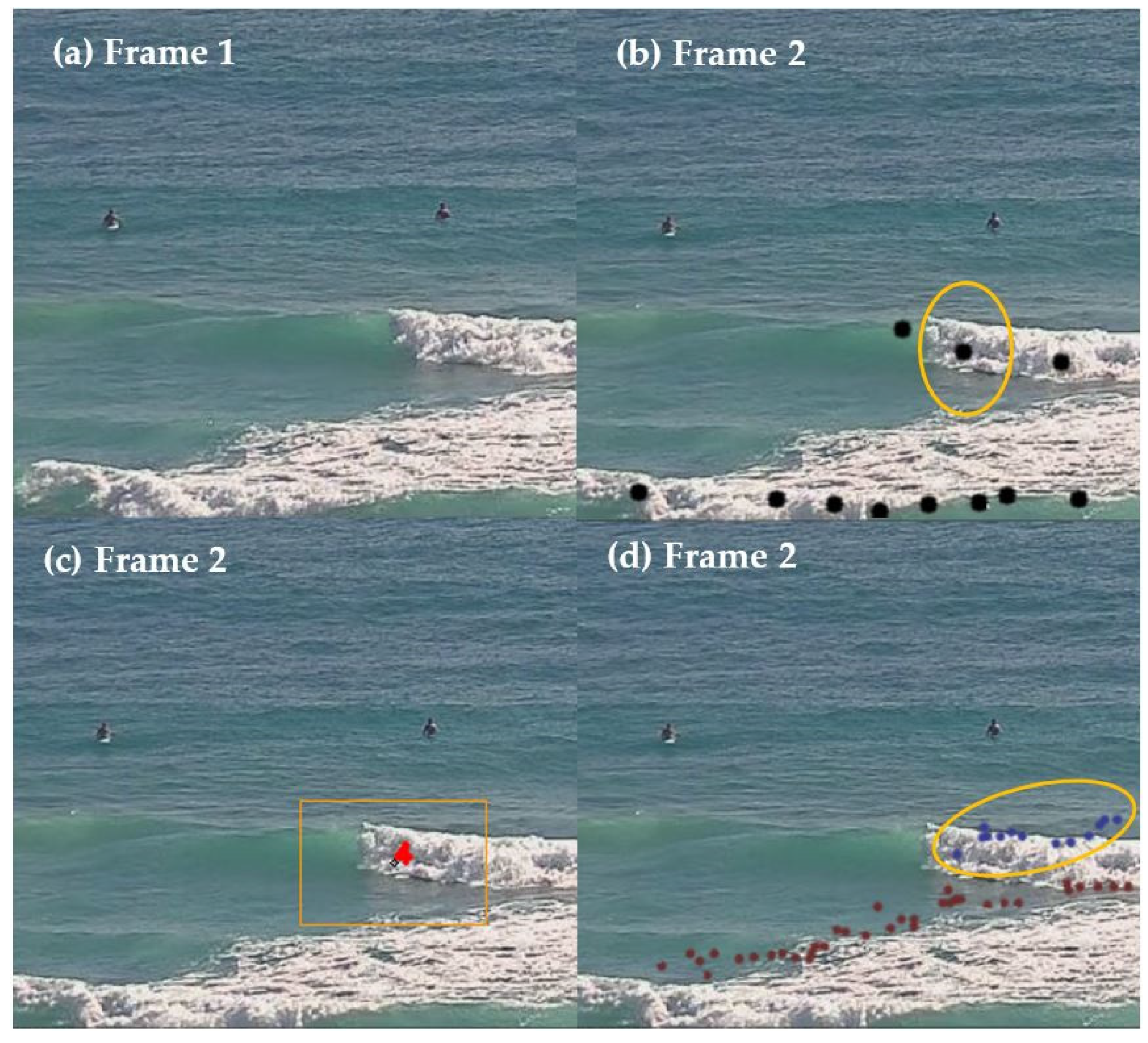
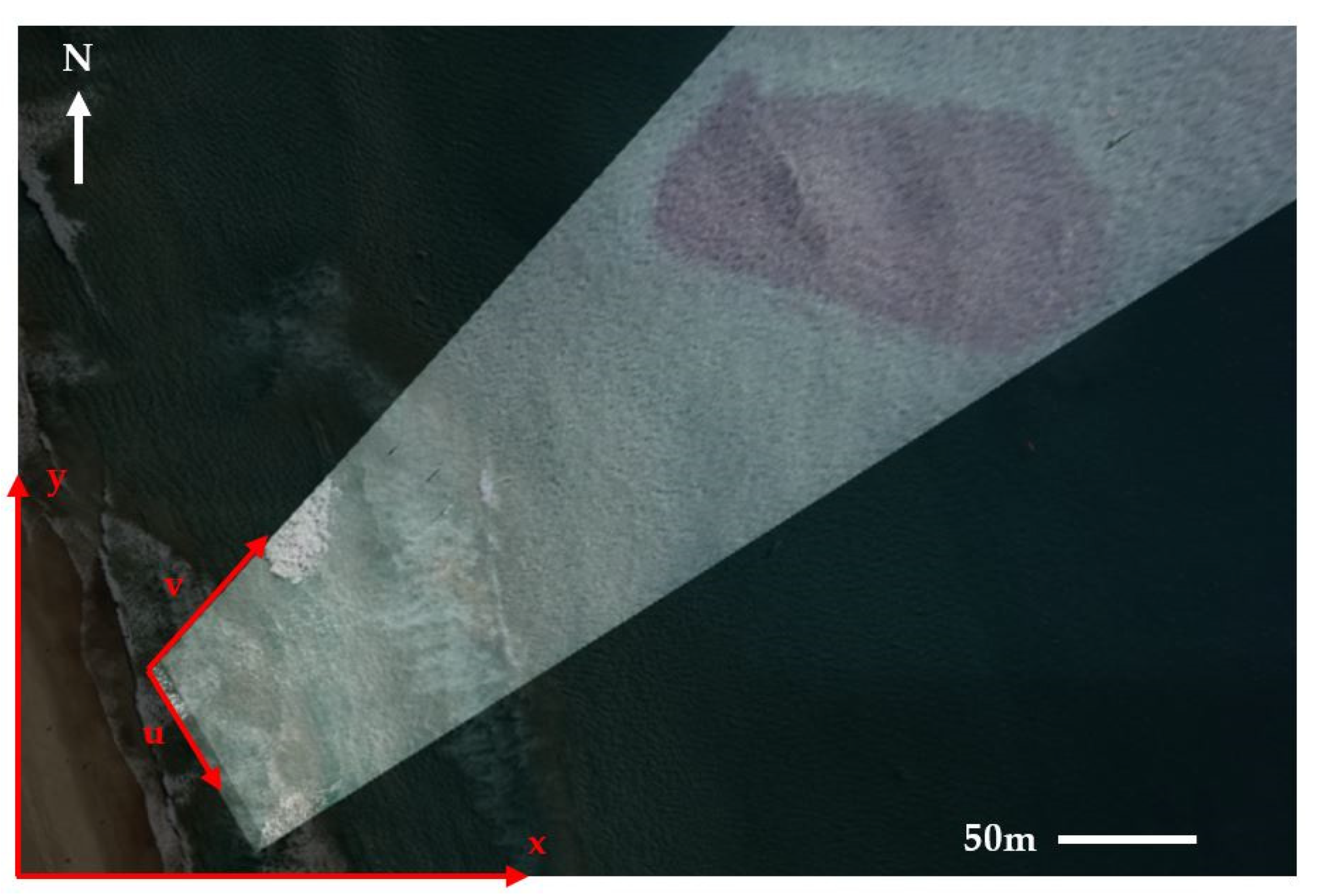
It must be noted that Equation (2) can be scaled; indeed, in projective geometry, vectors that are related through a scaling factor are deemed to be equivalent. For example, it is not guaranteed that the right hand will always end up with a 1 in the third component. However, so long as the third component is non-zero, the vector will represent a vector with third component 1 after appropriate scaling. When the third component is 0, this represents a ‘points at infinity’ relative to our setting, and does not have much relevance for our purposes. To determine the homography matrix values, at least 4 sets of corresponding u,v,x,y points must be determined [33]. The values in matrix H are found by an optimisation algorithm with set to 1 (in-built to the OpenCV library). The surveyed u,v,x,y points were obtained at a very low tide of 0 m LAT (Southport predicted tide data) by simultaneous video recording and surveying of the field of view with an RTK GPS mounted on a kayak. The GPS was mounted on a pole, such that the bottom of the pole at the kayak waterline provided visual data at the low tide level, and the top of the GPS provided visual data at the tide level +1 m. On the 17th of September 2020, a total of 10 GPS points were collected over and around the reef and around the adjacent nearshore region. A further 3 GPS points were collected at the mean water level at the shoreline. This survey methodology enabled generation of homography matrices for different tide levels from a single survey. The homography matrix for any tide was approximated by using sets of u,v,x,y points, where the v points were linearly interpolated or extrapolated, based on the 0 and 1 m LAT v points, according to the tide level. Figure 3 illustrates the effect of a homography matrix set for one tide level applied to every pixel in a camera image, overlaid on the map image.
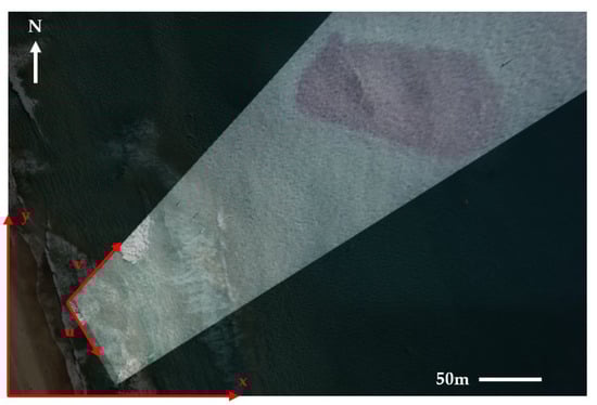
Figure 3.
Homography stretching applied to an image (note that the map image is not from the same date as the video image, so sand bars are not expected to line up). The reef is visible as the dark oblong in the upper right of the image.
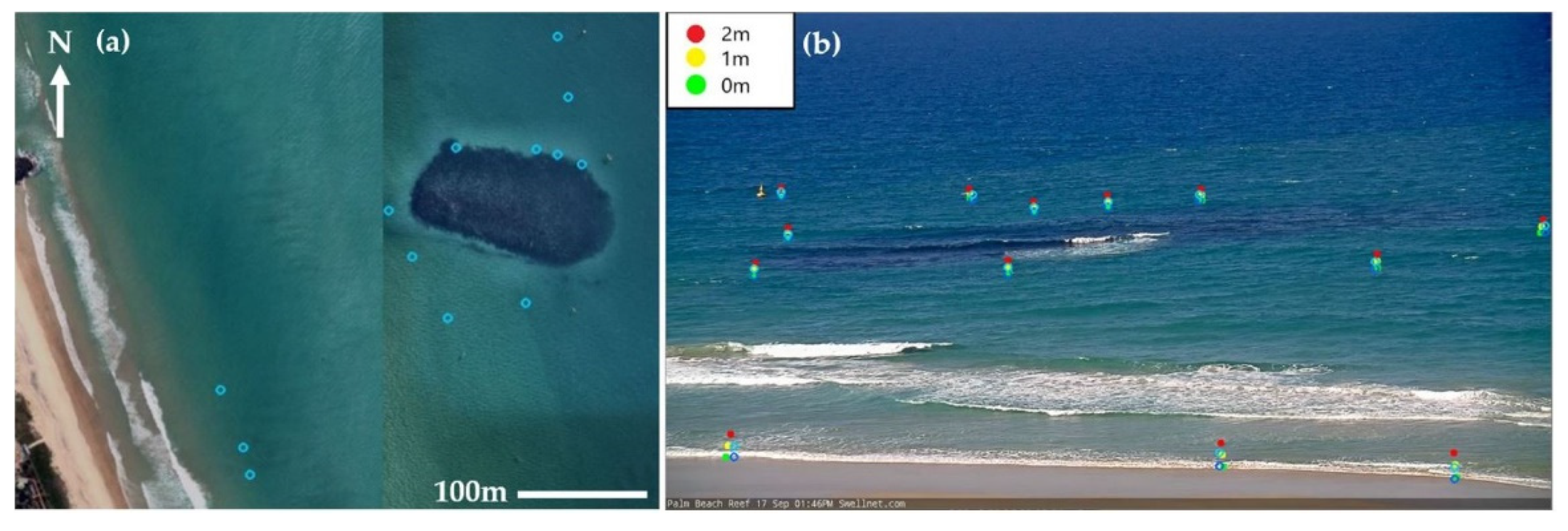
Figure 4 illustrates a visual verification of homography for different tides, where surveyed 0 and 1 m LAT points are represented by the unfilled circles on the map (blue, (a)) and on the image (dark blue and light blue, respectively, (b)). The filled circles in the image are all placed using the homography matrices calculated for each tide level, where the 0 and 1 m homography matrices were calculated from surveyed points and the 2 m homography matrix was calculated from extrapolated points. The homography technique works well, with the 0 and 1 m filled points almost all coinciding with the unfilled surveyed points. In (b), The bottom left and far right regions show some difference between points, because the application of planar homography is prone to greater potential errors at wider angles. The extrapolated 2 m filled points plot as expected, above the 1 m filled points with similar spacing according to the distance from the camera (i.e., closer points to the camera will have greater spacing between tide levels due to the perspective geometry). The pixels in the image had a rectified footprint of approximately 0.38 m/pixel on the reef and 0.37 m/pixel in the nearshore region.

Figure 4.
GPS verification map (a) and image (b). Unfilled blue points on the map show surveyed GPS points with corresponding points in the image (dark blue = 0 m LAT, light blue = 1 m LAT). Filled green, yellow and red points in the image were derived from the homography matrices for 0, 1 and 2 m LAT, respectively. Note that split aerial image (a) is not from the same date as (b), so shoreline sampled points in (b) are not supposed to plot on the shoreline in (a).
The homography matrices for different tides were independently verified on the 13th of January 2021, using data from the GPS surfing verification (Section 4.1). GPS points from surfing rides were compared with rectified locations of the surfers at the still water level (1/5 of wave face) in the video. The root mean square error (RMSE) between all GPS points and image rectified points was 17 m. The accuracy of the GPS watches used by the surfers in absolute position was ≈5 m (see Section 4.1 for details). Over the reef, the RMSE was 20 m and shoreward of the reef the RMSE was 13 m. This verification indicated a strong westerly bias (rectified points were further west than they should be), and therefore all rectified data in Section 4 onwards were shifted 10 m east to correct for this bias. By comparing camera snapshots at the same tide level on the 17 September 2020 and 17 October 2020, it was found that the camera had shifted field of view slightly to the left and appears to have maintained that position since. Given the NE orientation of the camera, a slight shift to the left is likely the cause for most of the required easterly bias shift of 10 m. Following the bias correction, RMSE changed to 11 m over the reef and 9 m in the nearshore region, with 10 m overall. Most of this remaining inaccuracy is suspected to be from the inaccuracy of the GPS watches. By comparing tides on the rectification day and on the GPS watch verification day, it was found the predicted tide levels varied at most 40 cm (nonlinearly) with the historical tide levels at the Southport tide gauge. The camera line of sight had a depression angle of approximately 5°, and therefore the projection error could be up to 5 m, which also could account for some of the inaccuracy in rectification. Only predicted tides are available for real-time processing applications, which is what is being tested in this work, and therefore predicted tides were still used. Further accuracy gains could also be made by simply using more rectification points for the homography. However, for the purpose of this work, the rectification accuracy of 10 m RMSE was acceptable.
2.6. Post Processing
The final data in rectified MGA94 coordinates were then processed to extract surf amenity metrics. Each individual wave peel track was used as proxy for the maximum possible ride length and duration of a surfer in the wave peel region. Average ride duration, average ride length, maximum ride length, average ride speed, ride directions and the ride rate were chosen as metrics for analysis. Ride duration was calculated as the time difference between the first and last point of each wave peel track. The ride rate was defined as the number of WPTs within a selected area, per minute, averaged over the full video duration (each video was of 10 min duration to ensure a near constant water level). The ride length was calculated as the distance between the first and last point of a WPT, after Gaussian smoothing. The Gaussian smoothing operation was performed to remove any jitter from the data and generate smooth tracks in x,y space. The standard deviation of the Gaussian smoothing found to minimise jitter whilst not severely reducing ride length was 4. The ride speed was simply the ride length divided by the ride duration and the ride direction was the bearing from start point to finish point.
3. Field Site and Data
3.1. Field Site
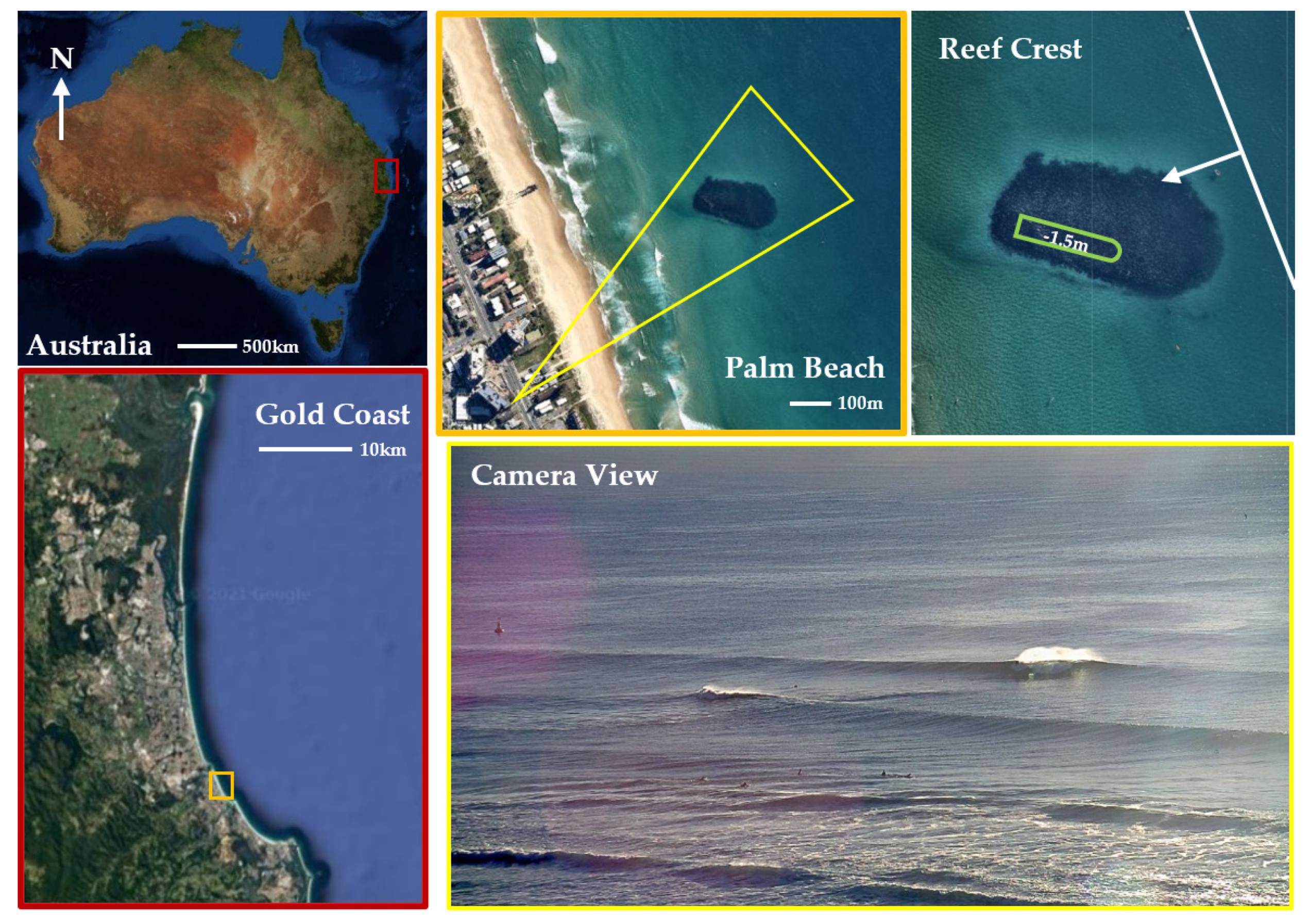
The WPT software was tested on a reef and in the nearshore region of Palm Beach, Gold Coast, Australia, on the 13 January 2021 (Figure 5). The Gold Coast regularly receives southerly storm swells during winter ( > 1.5 m, > 10 s) and occasional easterly and northerly cyclonic swells during summer ( > 3 m, > 10 s). The average significant wave height from 1995 to 2018 was 1.07 m and average peak period was 9.23 s (Tweed Heads wave buoy). The beach has a mixed tide system with tidal range of approximately 2 m and generally forms a longshore bar and trough system [34], with the occasional outer bar appearing after very large swell events.
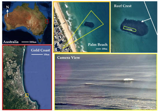
Figure 5.
Location of field site. The reef crest is shown in green and camera view is outlined in yellow (snapshot taken from 16 July 2020). White arrow in top right shows prevailing wave direction of 70°.
The reef is located 270 m offshore, with its crest submerged approximately 1.5 m below mean sea level. It is 160 m long, 80 m wide and contoured to form a crest 60 m long, aligned at an angle of 35° to the prevailing wave direction of 70° (as annotated in the top right of Figure 5). The reef was constructed of layered rocks, with 1–8 ton boulders forming the submerged armoured surface [35]. A permanent 1280 × 720 pixel CCTV camera set to capture at 10 frames per second (fps) was installed on a high-rise apartment approximately 40 m above sea level and 500 m SW of the reef, providing the camera view shown in yellow in Figure 5. All WPT data presented here were extracted from this video camera. The camera view shows the entirety of the water surface above the reef and some of the nearshore region. At very low tide the shoreline is visible in the image. On the 13th of January 2021, an outer bar was present which was a remnant bar from a very large easterly storm swell in December 2020 ( > 5 m). Waves at lower tides are expected to break along the reef crest, creating potential surf rides. This ride-producing aspect of the reef crest was used to informally verify the positioning of WPTs.
3.2. Dataset
Video recordings at 10 fps were obtained from 8 to 9 am and 12 to 2 pm, divided into 10 min clips. These data cover two distinct periods of the tide with different cloud cover and wave conditions. For both time periods, the significant wave height was close to 1.14 m with consistent peak period of 8 s. The peak wave direction was close to 70°, roughly perpendicular to the angle of the beach shoreline. During the morning time period, the sun was mostly out, with waves breaking in little wind. The tide was peaking at over 1.8 m LAT according to the 2021 Southport tide predictions. The afternoon time period was during mostly cloud cover with choppier waves due to increased winds, and the tide was falling from 1.02 m to 0.39 m LAT. All results and figures were rectified using the homography procedure outlined in Section 2.5. The analysis was based on 18 10 min records.
4. Results
This paper is concerned with the detailed analysis of the accuracy of the WPT method and how the results can be useful for surf amenity assessment, using data from one day (13 January 2021). Long-term WPT data gathered over several months from the CCTV camera will be the subject of a future analysis.
4.1. GPS Surfing Verification
The WPT data can be robustly verified and evaluated using tracks obtained from surfers equipped with GPS tracking devices. Data were collected from four different surfers—three using GPS wristwatches (Garmin Forerunner 235; Garmin Fenix 5X Sapphire; Garmin Fenix 5) and one with a bicycle GPS (Garmin Edge 500) inside a waterproof container, fixed to the tail pad of a surfboard. Only 10 of 17 GPS surfer tracks were used, with surfer tracks not in the wave peel region excluded (>3 m away based on visual inspection). Figure 6 illustrates the GPS points used for verification. Data from all the GPS devices were sampled at 1 Hz. The watches proved to be more reliable, where the bike computer in the waterproof case overheated and provided corrupted tracks after approximately 30 min of use. The absolute accuracy of one of the GPS watches was tested by repeated sampling at a fixed point over several days. There was significant variance in recorded position within each sample and between different samples of recorded data. Overall, the GPS watches provided data within a radius of approximately 4 m, with maximum deviations from the fixed position of up to 7 m, so any instantaneous position is deemed accurate within ≈5 m.

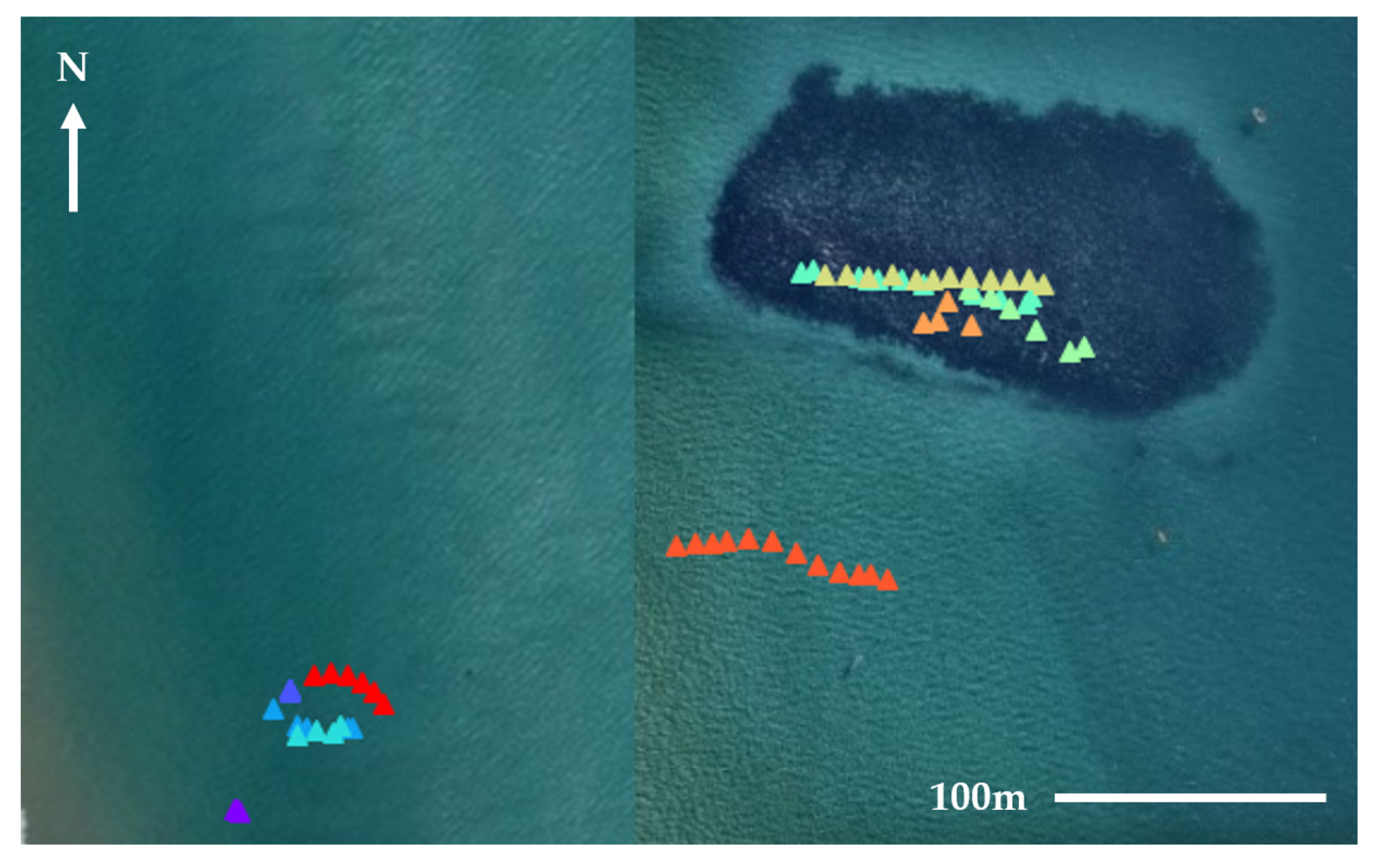
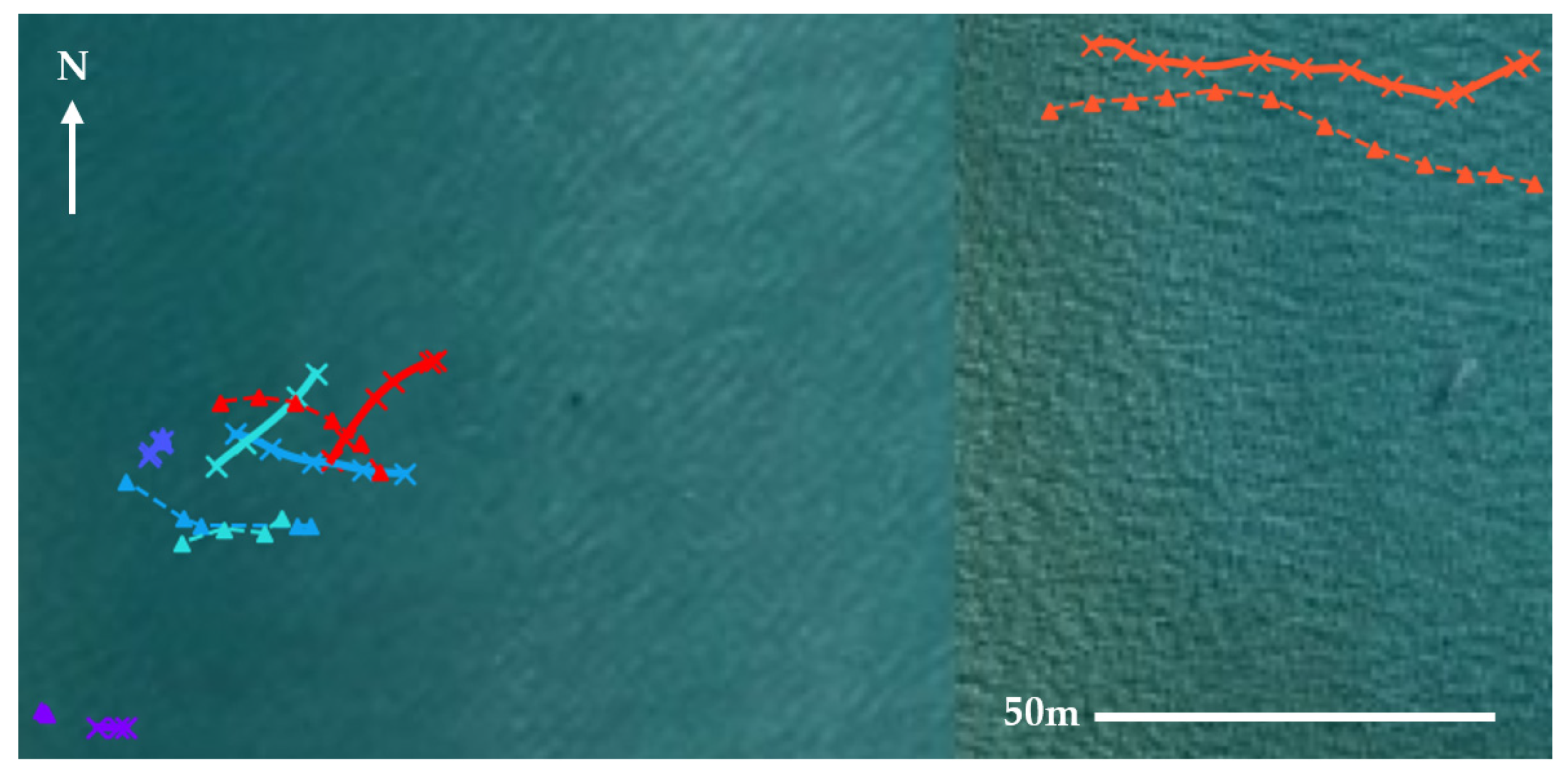
Figure 6.
Map of GPS surfer tracks, with different colours showing different tracks. The aerial image is split from 2 days (neither close to the 13 January 2021) to ensure a bland background to plot tracks in the nearshore region, while still allowing visual verification on the reef. Therefore, sand bars visible in the aerial image should be ignored with respect to the tracks.
GPS tracks in Figure 6 included two from the 8–9 am session (purple and dark blue) and eight from the 12–2 pm session. GPS tracks were collected from both right-hand rides (north-westerly rides) and left-hand rides (south-westerly rides). Tracks are separated as either on/beyond the reef or in the nearshore region (in lee of the reef). The orange GPS track in Figure 6 was from a rare break on the outer sand bar on this day, but most breaking waves in the nearshore region occurred over a nearshore bar. A detailed comparison of the reef WPTs and GPS surf tracks is illustrated in Figure 7, with differences and errors quantified in Table 1.

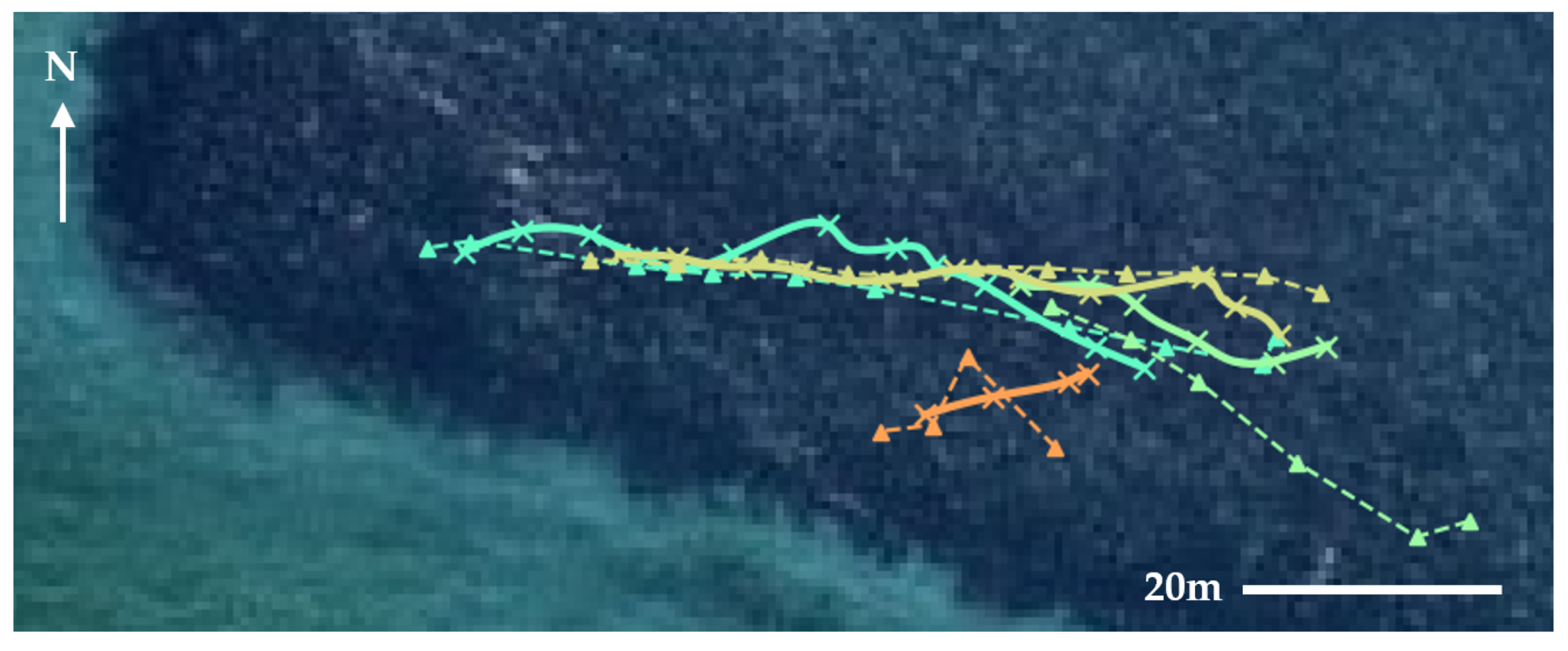
Figure 7.
Comparison of WPTs with GPS surfer tracks on the reef. -Δ- = GPS points; -×- = Gaussian-smoothed WPTs time synchronised with GPS points at 1 Hz.

Table 1.
GPS tracks compared with WPTs in the reef region.
All GPS tracks on the reef were right-hand rides. Rideable left-hand waves only occur on the reef occasionally and were not measured in this sampling interval. The overall RMSE value of 7 m was found comparing the GPS track points with the equivalent time synchronised Gaussian-smoothed WPT points. Both the Gaussian-smoothed WPT and GPS track ride lengths were calculated by the Euclidean distance between the first and last point of a track. The Gaussian-smoothed WPT ride lengths on the reef were found on average to be 17% less than the GPS ride lengths, with RMSE of 20%. This overall smaller length for WPTs is mostly an artefact of the Gaussian smoothing of the points. Gaussian smoothing was not removed since it was still required to reduce jitter between wave peel region classifications. The green track had significant error at the start which was suspected to be due to GPS inaccuracy.
A similar analysis for the nearshore region is illustrated in Figure 8, accompanied by Table 2. GPS tracks in the nearshore region were a mix of rights and lefts. The overall RMSE was 11 m. The Gaussian-smoothed WPT ride lengths on the reef were found on average to be 12% less than the GPS ride lengths, excluding the aqua blue left track which had a greater WPT length than GPS length. Including the aqua blue track, the RMSE of the ride lengths was 19%. Similar to the reef results, Gaussian smoothing produced a slightly shorter WPT length, and therefore WPT ride lengths are considered a conservative measure overall.

Figure 8.
Comparison of WPTs with GPS surfer tracks in the nearshore region. -Δ- = GPS points; -×- = Gaussian-smoothed WPTs time synchronised with GPS points at 1 Hz.
Table 2.
GPS tracks compared with WPTs in the nearshore region.
For the reef and nearshore region, the RMSE of WPTs was 9 m, which is good given the ≈5 m accuracy of the GPS watches. The majority of WPT ride lengths were shorter than GPS tracks, with RMSE of 20% overall. Further decomposition of the possible sources of inaccuracy was performed through comparing GPS tracks with rectified manually extracted surfer tracks from the video (to estimate rectification accuracy), comparing rectified manually extracted surfer tracks from the video with rectified manually extracted WPTs (to estimate ability of surfer to stay in the wave peel region), and comparing rectified manually extracted WPTs with rectified algorithm extracted WPTs (to estimate the accuracy of the algorithm). Whilst not entirely summative, this suggests that approximately 50% of the differences between the WPT and GPS tracks was contributed by rectification procedures, 15% from surfers deviating from the wave peel region and 35% from inaccuracy of the algorithm. The timings of the WPTs (sampled at 10 Hz) and GPS points (sampled at 1 Hz) were well synchronised and the tracks generally aligned well in plan. Therefore, metrics for ride duration are deemed accurate to within approximately ±1 s. The resolution of the algorithm depends on the frame rate of the video and the rectified field of view of the camera. In this instance, the time resolution was 0.1 s (10 fps) and spatial resolution was within 1 m (according to Section 2.5).
4.2. Metrics Obtained from Wave Peel Tracks
Some WPT metrics describing the surf amenity have been separated into hourly tidal ranges of high, mid and mid–low (8–9 am, 12–1 pm and 1–2 pm, respectively). The variation in tidal range during the falling tide for the 12–1 pm and 1–2 pm data sets was larger, at approximately 0.3 m, compared to the 0.03 m range for the 8–9 am results obtained at high tide. Significant wave height, peak period and wave direction remained relatively constant throughout the day. Table 3 shows both the relevant weather data from the local wave buoy and predicted Southport tides, and associated metrics obtained from the WPTs.
Table 3.
Summary of WPT data over each hour.
The most notable trend in the data is that for all tides, the average ride duration and average ride length on the reef is greater than in the nearshore region. The average ride duration on the reef is approximately 1.5-fold greater than in the nearshore region and the average ride length is approximately 2-fold greater on the reef. These results agree with expectations, given that the reef has a long, fixed crest for waves to break along, providing longer rides than a natural sandy beach break. The average ride speed was often faster over the reef than in the nearshore region, likely due to waves breaking in slightly deeper water on average than the nearshore region. Maximum ride length generally increased with the falling tide (with the exception of the mid tide in the nearshore region) as the depth reduced to increase shoaling and breaking over the reef. No significant correlation between the maximum wave height at the wave buoy and maximum ride lengths was observed in these data (not shown), but variation of the maximum wave height over the observed period was less than 0.5 m.
One potential problem with the WPT approach in the nearshore region was the edges of the field of view causing some WPTs to be cut short. The smallest width of the nearshore region in the field of view was approximately 80 m in the cross-shore direction. The lengths of WPTs in this region in the cross-shore direction were typically much smaller than this length (most in the range of 7–36 m). To check the influence of the field of view cut off, the average metrics were found for the middle third of the nearshore width in the cross-shore direction, where WPTs that started outside this region were excluded and all WPTs up to the boundary of the reef were included. Average ride length, duration and speed only rose by 4%, 1% and 3%, respectively, which was a very small difference. If the maximum nearshore width in the cross-shore direction was significantly smaller, that may have led to problems but the chosen field of view was acceptable.
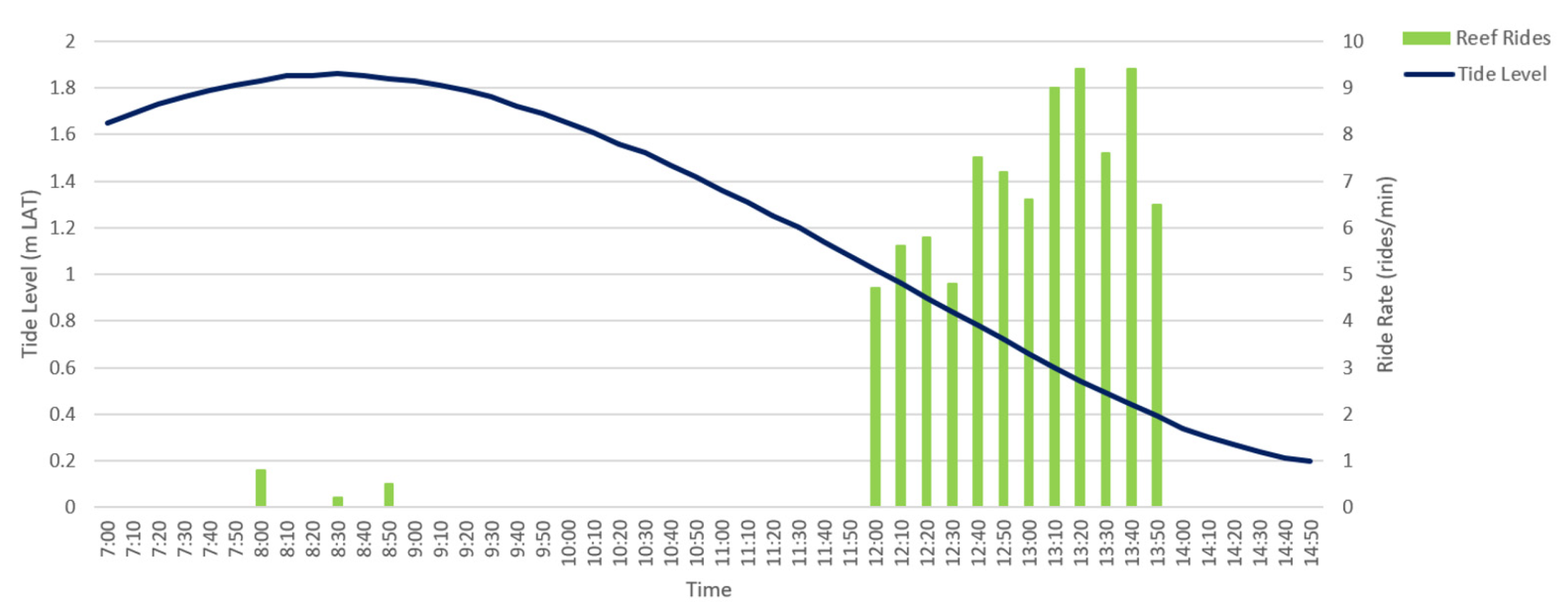
Figure 9 illustrates that ride rate was inversely proportional to the tide level over the reef. A small portion of the midday nearshore ride rates was due to choppier wind affected waves, causing more wave peel regions to be present; however, these winds were consistent across the midday time period. While these WPTs had lower duration and shorter length, this did not affect the data significantly.

Figure 9.
Tide level vs. ride rates over the reef (8–9 am and 12–2 pm only).
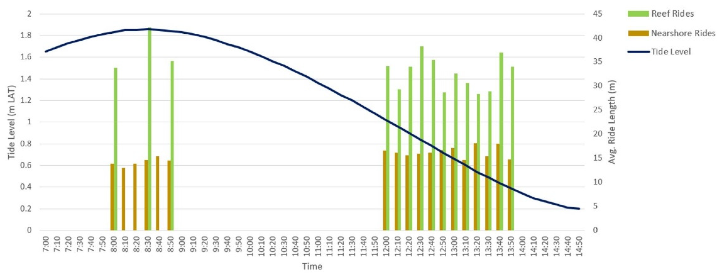
Figure 10 illustrates the consistency of the long ride lengths over the reef, despite a lower ride rate at a higher tide level. This aligns with expectations, where only the larger waves break on the reef crest due to depth limited breaking. It was also expected that many more rides would ‘close out’ in the nearshore region compared to the reef. Average ride lengths increased in the nearshore region by approximately 4 m at lower tide, which was likely due to the addition of waves breaking on the outer bar just inside of the reef.

Figure 10.
Tide level vs. WPT average ride lengths in the nearshore and reef regions.
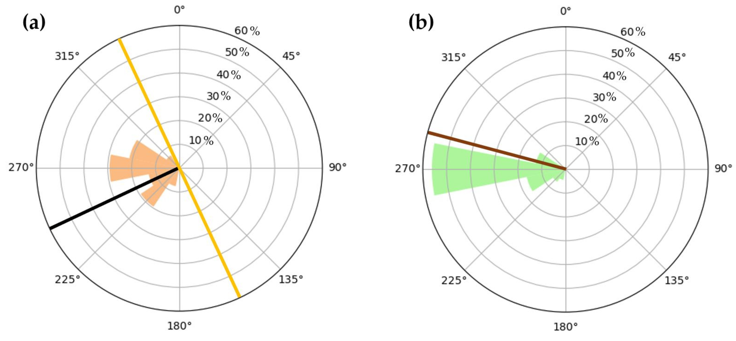
WPT directions provided additional insight into surf amenity. The proportions of ‘right’ and ‘left’ surfing rides at a surf break is important knowledge for surfers. In Figure 11a illustrates the distribution of WPT directions in the nearshore region. The lefts were in the SW–S directions, rights in the W–NW directions and the normal of the shoreline was WSW. There was a higher proportion of rights which was likely due to the additional rights on the outer sand bank exposed at lower tide levels. This mix of left and right surfing rides was also observed during the GPS surfing verification exercise. The distribution of WPT directions was much more consistent over the reef (Figure 11b), with high density near the direction of the reef crest. Most WPTs on the reef had direction E rather than ENE because they started breaking on the north side of the crest and finished breaking on the south side of the crest (see Figure 12b).

Figure 11.
WPT direction distributions for nearshore region (a) and reef (b). For the nearshore region, the approximate shoreline angle is shown in yellow, with shoreline normal in black. For the reef, the reef crest angle is shown in brown.

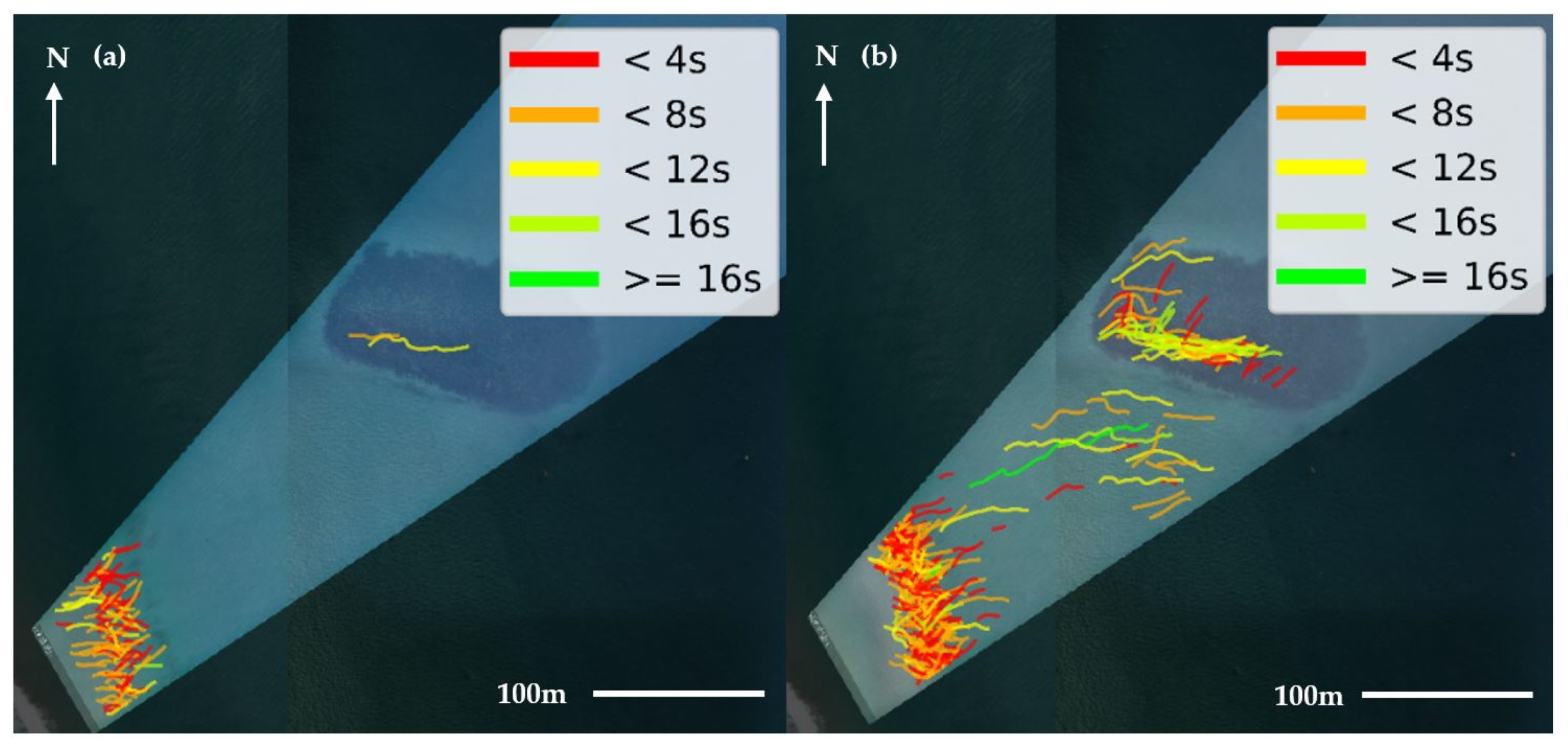
Figure 12.
Durations maps for tracked rides between 8:30 am and 8:40 am at tide = 1.86 m LAT (a) and 12:10 pm and 12:20 pm at tide = 0.96 m LAT (b).
One of the most insightful representations of the WPT data is a ride durations map, where WPTs are overlaid and colour coded according to ride duration. Additionally, a rectified time-exposure image of the processed 10 min video clip is overlaid on an aerial image. In Figure 12a illustrates an example ride durations map for a short period of data from 8:30 am to 8:40 am at a tide level of 1.86 m LAT. It must be noted that the start of each WPT will not represent the initial breakpoint, but rather when either a right or a left wave peel region is fully formed. The time and length of a track from initial breakpoint to fully formed wave peel region are very small however (≈1 s, 3 m). The WPTs in the nearshore region of Figure 12a reveal the position of a sand bar. The dark grey/black spots from the time-exposure image show the positioning of the surfers which is commonly at the breakpoint of the larger waves. There were only a few WPTs recorded on the reef, which shows good visual agreement with the location and orientation of the reef crest. In Figure 12b shows the WPTs for a video clip from 12:10 pm to 12:20 pm at a lower tide level of 0.96 m. With shallower water over the reef and nearshore sand bars, many more rides occur, and the start of the tracks (fully formed wave peel region positions) shift further seaward. The outer sand bar shoreward of the reef became shallow enough for wave breaking, revealed by the appearance of WPTs in this region. There were also a small number of shorter WPTs directed SW over the reef. These small-length and -duration SW tracks near the breakpoint indicate a left ride. The small-length and -duration tracks near the middle and W side of the reef also represent left rides. The slightly longer rides on the N tip of the reef were wide breaking right rides.
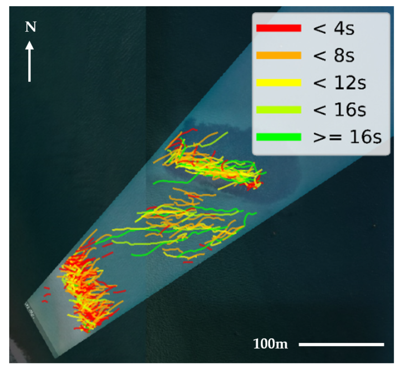
Figure 13 shows a durations map for data from 1:40 pm to 1:50 pm, at an even lower tide level of 0.44 m. The WPTs show greater breaking activity, again shifted further seaward in the nearshore region, on the outer sand bar and on the reef. There are three short WPTs further landward than the well-defined nearshore sand bar. After reviewing the processed video, these were found to represent very small unsurfable WPTs near the swash zone and had negligible influence on average WPT metrics.

Figure 13.
Durations map for tracked rides between 1:40 pm and 1:50 pm at tide = 0.44 m LAT.
5. Discussion
The automated wave peel tracking methodology outlined here has proven effective for assessing the surf amenity of a reef and nearshore region. The ride metrics demonstrate that ride lengths were longer on the reef compared to the nearshore region for the same incident offshore wave conditions. The WPT data show ride rate inversely proportional to tide level over a fixed depth structure (reef), as expected from depth limited breaking. Plotting WPTs on a spatial map reveals how ride location and direction vary at different tide levels on the reef. These plots also reveal the positions of nearshore and outer sand bars. This work has shown that a standard CCTV camera can be used effectively for extracting WPT data. However, the WPT approach is not limited to fixed CCTV cameras and can be used with any high-resolution camera at a high elevation position [36]. This flexibility, and the ability of the methodology to track WPTs both over well-defined fixed structures and over natural sandbars, enables the proposed WPT methodology to be used to provide a baseline evaluation of the amenity of a natural surf break before any coastal developments are implemented. Following construction, the WPT methodology can then be used at the same location for an objective and quantitative assessment of any changes to the surf amenity.
The resolution of the WPT algorithm is dependent on the frame rate of videos and rectified field of view of the camera, in this work 0.1 s and 1 m, respectively. Absolute position of the WPTs is less accurate, but acceptable. All rectified tracks required a 10 m bias offset before WPTs were processed to better align with GPS surfing tracks. This was likely due to a slight camera shift following rectification. For future applications it is suggested that the camera be setup with a land survey point in the field of view so that any slight camera shifts can be quantified. Remaining post bias offset rectification inaccuracy was likely from using predicted rather than historical tides for rectification. The GPS surfing watches (≈5 m accuracy) were also used to verify the WPT software to 9 m RMSE in terms of absolute position and ride lengths to 20% RMSE of GPS-measured ride lengths. Most WPT ride lengths were slightly shorter than GPS ride lengths. Most of the inaccuracies were likely from rectification (post bias offset) and the WPT algorithm accuracy, with only a small amount of error from the difference in surfer GPS tracks with the true wave peel region. Rectification accuracy could be improved through a greater number of rectification points. It could also be improved by using historical tide readings; however, one aim was to provide data in real time, so predicted tides must be used in that instance. The cross-shore width of the field of view was found to be wide enough such that cut off WPTs at the boundaries did not significantly influence the calculated average WPT surf amenity metrics. To ensure this does not become an issue for other applications, it is suggested that the cross-shore width of the field of view should be at least twice the cross-shore length of the larger WPTs expected.
Given the nature of wind and swell waves, and the complexity of different surf and weather conditions, the metrics and maps created from the WPT software require some care in interpretation. Firstly, the WPTs do not always start from the breakpoint, but rather start when right or left wave peel regions are fully formed. Windy conditions can increase the number of wave peel regions, but not all will be rideable. Some spilling breaker WPTs in the videos are not necessarily rideable (dependent on surfer skill). Additionally, WPTs can sometimes be identified very close to the shoreline from waves breaking at the swash zone, which again are not surfable. The classification accuracy of wave peel regions was found to be practically effective, with an accuracy of 87.5% from assessing against an external test set. However, some notable misclassifications were observed. Wakes of boats and jet skis can be tracked in error and some very strong glare can also lead to false tracks on a wave face. The video recordings processed for this paper were not affected by any of these issues apart from one boat wake (this was easily identified in the 8:40–8:50 am video, see Supplementary Materials for video playlist). Some of these issues have been identified from running the WPT software on the same camera over 4 months. For a long-term application of the WPT approach for research purposes, it is suggested that video recordings be quality checked for possible misclassifications before using the WPT data, as done for this work. For real-time production, this is not possible, but given the relatively rare occurrences or predictability of these issues they do not negate the value of the methodology.
Future Improvements and Applications
Future improvements to the current WPT methodology will be focused on sensitivity analysis of the tracking cost function parameters and other parameters, improving spatial accuracy, and training a more robust CNN classifier against misclassifications. The tracking cost function (Equation (1)), motion detection, classification and post processing parameters give ample control of the WPT algorithm to suit different beach environments (see video playlist in Supplementary Materials for examples); however, having a large number of parameters is not ideal. Sensitivity analysis can be performed in future work to investigate where simplifications in parameters could be made. The CNN model can be improved with regression localisation for more precise WPT centring, and the training dataset can be increased for robustness to misclassifications. Additionally, unsurfable wave peel region images can be added to the training dataset to prevent unsurfable WPTs being produced. A further aim is to develop a regression CNN trained for determining relative wave heights and wave crest angles from each wave peel region. This approach could complement existing methods to estimate surf zone wave heights from remotely sensed video [15,21,37]. To further increase rectification accuracy, post processing can use actual historical tides, including coastal trapped waves and surges, instead of forecast tide predictions (in the scenario where real-time WPT data are not necessary).
New applications to coastal engineering research topics are possible with the existing methodology and with the noted future improvements. The WPT duration maps clearly reveal the potential for estimating water depths from the tracks (depth inversion). Further research will focus on using WPT to identify breakpoints, wave heights and wave crest angles, to be applied to the CERC equation [38] for estimating longshore sediment transport rate. Finally, the WPT approach has been successfully applied to laboratory scale models of both natural bathymetry and an artificial surfing reef in a 3D wave basin. This is being compared to corresponding numerical model results to assist the design of a new artificial surfing reef. In this manner, the WPT approach and the present methodology can be used to validate wave breaking processes through the complete engineering design process of numerical modelling, physical modelling and field assessment.
Supplementary Materials
The following are available online at https://www.mdpi.com/article/10.3390/rs13173372/s1. The WPT metrics data, WPT durations maps and paper figures are provided in the supplementary data zip file. Videos of the WPT software processing all the data before the bias offset can be found in the following YouTube playlist. The playlist also includes unrectified WPT software processing of other beach videos. https://youtube.com/playlist?list=PLJSOHg6_zTjUk3nUpN0IAfEGv8Xxsw7RF, accessed on 18 August 2021.
Author Contributions
Conceptualisation, M.T. and T.E.B.; methodology, M.T. and I.Z.; software, M.T.; validation, M.T., T.E.B. and E.W.; formal analysis, M.T., T.E.B. and E.W; data curation, M.T.; writing—original draft preparation, M.T.; writing—review and editing, T.E.B., E.W. and I.Z.; supervision, T.E.B.; funding acquisition, E.W. All authors have read and agreed to the published version of the manuscript.
Funding
This research was funded by an Australian Government Research Training Program Scholarship and the camera was sourced by the City of Gold Coast.
Institutional Review Board Statement
Not applicable.
Informed Consent Statement
Informed consent was obtained from all subjects involved in the study. Written informed consent has been obtained from the patients to publish this paper.
Data Availability Statement
The data are available on request.
Acknowledgments
The authors would like to thank Heiko Loehr and James Lewis from Bluecoast Consulting Engineers for their involvement in providing engineering critique and feedback during stages of development of the WPT software. They have also played a crucial part in the rectification and GPS surfing verification exercises. The authors wish to thank Jord Wiegerink for his involvement in the GPS surfing verification exercise and labelling of the external test set of wave peel regions, Alejandro Astorga Moar for his help in the rectification exercise. The authors would also like to thank Ben Matson from Swellnet who has enabled this research to continue through the use of a live beach camera. Thanks to James Fyvie and Zoe Elliot Perkins for allowing the funding of this project from The City of Gold Coast. Thanks to Simon Brandi Mortensen for his guidance for the WPT idea when it was in its infancy. Thanks to Alex Atkinson and Nick Naderi for labelling of the external test set of wave peel regions and the opportunity to test the WPT software in the wave basin at the Queensland Government Hydraulics Laboratory. Thank you to Darrell Strauss for helpful feedback for WPT data visualisation. Thank you to the State of Queensland, Department of Environment and Science, for supply of the Palm Beach wave buoy data, Tweed Heads wave buoy data and Southport tide data (historical and predicted). https://creativecommons.org/licenses/by/4.0/, accessed on 18 August 2021.
Conflicts of Interest
The authors declare no conflict of interest. The funders had no role in the design of the study; in the collection, analysis, or interpretation of data; in the writing of the manuscript, or in the decision to publish the results.
Appendix A
A blob masking iteration process is implemented to handle the case when a very large blob is detected. If an entire breaking bore is represented by a blob, then the blob centre will not accurately capture any possible wave peel region positions. In this case, the blob has to be split, which is performed as follows. After the blob centre is detected, the region of the blob around the centre, spanning the bounding box size, is masked out. The motion mask, capturing the entire bore, now has the middle of the mask whited out, leaving two medium sized blobs. The blob detection iteration process then continues to repeat until no more blobs greater than the minimum blob size are detected. This approach means the blobs at the edge of the bore are close to the wave peel regions and can then be classified by the CNN.
Appendix B
To train the successful CNN for wave peel region classification, 672 wave peel region and 661 non-wave peel region snapshots were labelled. Variation in labelled wave peel regions included left-hand and right-hand wave peel regions, surfed waves, non-surfed waves, dirty water, clean water, dark water, dull lighting, bright lighting, varying wave sizes, glare, plunging, spilling, foamy and wave peel regions breaking near rocks, with some examples illustrated in Figure A1. Variation in labelled non-wave peel regions included bores with no wave peel region, surfers with no wave, glare on a wave crest, feathering waves and combinations of these with the previously mentioned conditions.

Figure A1.
Examples of labelled classification images as used for training. Labelled images did not need to be very high resolution.
Figure A1.
Examples of labelled classification images as used for training. Labelled images did not need to be very high resolution.
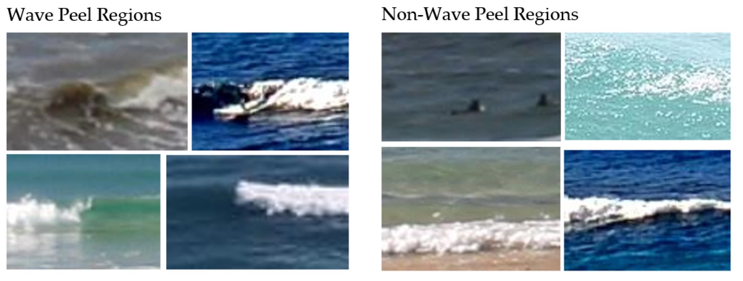
Snapshots were taken from the reef and nearshore region in this work, Palm Beach beach break near Currumbin Alley, Snapper Rocks point break, Duranbah beach break, Currumbin Alley point break, and Rainbow Bay point break, all at the Gold Coast. None of the labelled images were from the 13th January 2021 video footage used in this work to prevent bias. The labelled snapshots varied in size and dimensions, but were kept to a landscape ratio of approximately 3:2 (length:height) to simplify the data labelling process. The data were resized into 52 × 52 pixel images for the CNN. It was found that this image size was efficient for a feed-forward pass of the CNN whilst still allowing practical classification accuracy. Data augmentation involved flipping each image from left to right, and therefore a total of 2666 images were used for training the CNN. The CNN classifier design was a small VGGnet style architecture [39], illustrated in Figure A2. Only two VGGnet convolutional blocks were used, fed into two fully connected layers with dropout added to prevent overfitting. Common and practical design choices for using Tensorflow [40] were used for other aspects of the CNN. For binary classification a sigmoid activation function was used in the output layer. The ReLU activation function was used for all hidden layers and a binary cross entropy loss function was chosen.
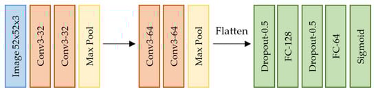
Figure A2.
CNN classifier architecture.
Figure A2.
CNN classifier architecture.
To evaluate the performance of the CNN classifier and confirm that the labelled wave peel regions used for training were not biased, a separate dataset of 100 wave peel regions and 100 non-wave peel regions were labelled independently by 3 people (including the first author). A 3-way agreement of over 91% was found which shows the consistency in manual classification of wave peel regions. This set of 200 waves is referred to as the external test set. The external test set included a higher proportion of more challenging images than the labelled training data. The labelled training data were randomly split into 76.5% training data, 8.5% validation data and 15% test data. Note, this is not the external test set, rather it is a second validation set for Tensorflow. Training accuracy was 98.47% and test accuracy was 94.91%, which shows initial signs of generalisation of the model. Table A1 shows the confusion matrix from the external test set of 100 wave peel regions and 100 non-wave peel regions.
Table A1.
CNN classifier confusion matrix.
Table A1.
CNN classifier confusion matrix.
| N = 200 | Predicted Wave Peel Region | Predicted Non-Wave Peel Region |
|---|---|---|
| Actual Wave Peel Region | TP1 = 95, 91 | FN 1 = 5, 9 |
| Actual Non-Wave Peel Region | FP1 = 25, 16 | TN 1 = 75, 84 |
1 The first value is with 0.5 confidence threshold; the second value is with 0.9 confidence threshold.
False negatives are very rare and are not detrimental to the algorithm, since the relatively high frame rate allows some contingency. Initially, the number of false positives was fairly high, a large contributor to them was foamy water and almost complete bores. To minimise false positives, the confidence threshold was set to 0.9 instead of 0.5. The second values in Table A1 show that the false positives dropped with this new confidence threshold. Most remaining false positives were exposed rocks and glare which were not present in the footage for this work. External test set accuracy using the confidence threshold of 0.9 was 87.5% which was practically acceptable for WPT (see results in Section 4).
References
- Smith, J. Another Fine Wave Destroyed! (This Time, In Bali). Available online: https://stabmag.com/news/another-perfect-wave-destroyed-this-time-in-bali/ (accessed on 21 June 2021).
- Scarfe, B.; Healy, T.; Rennie, H. Research-Based Surfing Literature for Coastal Management and the Science of Surfing—A Review. J. Coast. Res. 2009, 25, 539–557. [Google Scholar] [CrossRef]
- Endangered Waves. Available online: https://www.surfrider.org.au/programs/endangered-waves/ (accessed on 21 June 2021).
- Mucha, N. It’s Official Gold Coast is the 8th World Surfing Reserve. Available online: http://www.goldcoastworldsurfingreserve.com/ (accessed on 21 June 2021).
- Walker, J.; Palmer, R.; Kukea, J. Recreational surfing on Hawaiian reefs. In Proceedings of the 13th Coastal Engineering Conference, Vancouver, BC, Canada, 10–14 July 1972; pp. 2609–2628. [Google Scholar]
- Scarfe, B.; Elwany, M.; Mead, S.; Black, K. The science of surfing waves and surfing breaks: A review. In Proceedings of the Artificial Surfing Reefs 2003: The 3rd International Conference, Raglan, New Zealand, 23–25 June 2003; pp. 1–12. [Google Scholar]
- Black, K.; Mead, S. Design of the Gold Coast Reef for Surfing, Public Amenity and Coastal Protection: Surfing Aspects. J. Coast. Res. 2001, 29, 115–130. [Google Scholar]
- Lewis, J.; Hunt, S.; Evans, T. Quantification of Surfing Amenity For Beach Value And Management. In Proceedings of the Coastal Conference, Forster, Australia, 11–13 November 2015. [Google Scholar]
- Scarfe, B. Categorising Surfing Manoeuvres Using Wave and Reef Characteristics. Master’s Thesis, The University of Waikato, Hamilton, New Zealand, 2002; p. 181. [Google Scholar]
- Moores, A. Using Video Images to Quantify Wave Sections and Surfer Parameters. Master’s Thesis, The University of Waikato, Hamilton, New Zealand, 2001; p. 143. [Google Scholar]
- Weppe, S.; Shand, T. Modelling Surf Break Wave Mechanics with SWASH—An application to Mangamaunu Point Break (Kaikōura, New Zealand). In Proceedings of the Australasian Coasts & Ports Conference, Hobart, Australia, 10–13 December 2019; pp. 1218–1225. [Google Scholar]
- Mortensen, S. Protecting and Enhancing Surf Amenity. Available online: https://www.dhigroup.com/global/news/2015/4/protecting-and-enhancing-surf-amenity (accessed on 21 June 2021).
- Aagaard, T.; Holm, J. Digitization of Wave Run-up Using Video Records. J. Coast. Res. 1989, 5, 547–551. [Google Scholar]
- Yoo, J.; Fritz, H.; Haas, K.; Work, P.; Barnes, C. Depth Inversion in the Surf Zone with Inclusion of Wave Nonlinearity Using Video-Derived Celerity. J. Waterw. Port Coast. Ocean Eng. 2011, 137, 95–106. [Google Scholar] [CrossRef]
- Shand, T.; Bailey, D.; Shand, R. Automated Detection of Breaking Wave Height Using an Optical Technique. J. Coast. Res. 2012, 28, 671–682. [Google Scholar]
- Stringari, C.; Harris, D.; Power, H. A novel machine learning algorithm for tracking remotely sensed waves in the surf zone. Coast. Eng. 2019, 147, 149–158. [Google Scholar] [CrossRef]
- Andriolo, U. Nearshore Wave Transformation Domains from Video Imagery. J. Mar. Sci. Eng. 2019, 7, 186. [Google Scholar] [CrossRef] [Green Version]
- Ellenson, A.; Simmons, J.; Wilson, G.; Hesser, T.; Splinter, K. Beach State Recognition Using Argus Imagery and Convolutional Neural Networks. Remote Sens. 2020, 12, 3953. [Google Scholar] [CrossRef]
- Buscombe, D.; Carini, R. A Data-Driven Approach to Classifying Wave Breaking in Infrared Imagery. Remote Sens. 2019, 11, 859. [Google Scholar] [CrossRef] [Green Version]
- Stringari, C.; Guimarães, P.; Filipot, J.; Leckler, F.; Duarte, R. Deep neural networks for active wave breaking classification. Sci. Rep. 2021, 11, 3604. [Google Scholar] [CrossRef] [PubMed]
- Buscombe, D.; Carini, R.; Harrison, S.; Chickadel, C.; Warrick, J. Optical wave gauging using deep neural networks. Coast. Eng. 2020, 155, 103593. [Google Scholar] [CrossRef]
- Fung, J. Vision-Based Near-Shore Wave Tracking and Recognition for High Elevation and Aerial Video Cameras. Available online: https://github.com/citrusvanilla/multiplewavetracking_py (accessed on 21 June 2021).
- Kim, J.; Kim, J.; Kim, T.; Huh, D.; Caires, S. Wave-Tracking in the Surf Zone Using Coastal Video Imagery with Deep Neural Networks. Atmosphere 2020, 11, 304. [Google Scholar] [CrossRef] [Green Version]
- Bryan, K.; Davies-Campbell, J.; Hume, T.; Gallop, S. The Influence of Sand Bar Morphology on Surfing Amenity at New Zealand Beach Breaks. J. Coast. Res. 2019, 87 (Suppl. 1), 44–54. [Google Scholar] [CrossRef]
- Shand, T.; Weppe, S.; Quilter, P.; Short, A.; Blumberg, B.; Reinen-Hamill, R. Assessing the effect of Earthquake-Induced Uplift and Engineering Works on a Surf Break of National Significance. In Proceedings of the ICCE, Online, 31 December 2020; Volume 36, p. 23. [Google Scholar] [CrossRef]
- Mckenzie, S.; Green, R. Gnarometer Surfcam Live Inspector. In Proceedings of the International Conference on Image and Vision Computing, Auckland, New Zealand, 19–21 November 2018; pp. 1–6. [Google Scholar] [CrossRef]
- Freeston, B. Real-Time Smart Monitoring and Prediction of Recreational Use and Environmental Data from Ocean Facing CCTV Cameras—Surfzone.ai. Available online: https://www.surfzone.ai/ (accessed on 21 June 2021).
- Patterson, D. Low Cost Visual Determination of Surfzone Parameters. Master’s Thesis, University of Queensland, Brisbane, Australia, 1985. [Google Scholar]
- OpenCV, SimpleBlobDetector Class Reference. Available online: https://docs.opencv.org/3.4/d0/d7a/classcv_1_1SimpleBlobDetector.html (accessed on 21 June 2021).
- LeCun, Y.; Bottou, L.; Bengio, Y.; Haffner, P. Gradient-based learning applied to document recognition. Proc. IEEE 1998, 86, 2278–2324. [Google Scholar] [CrossRef] [Green Version]
- Bewley, A.; Ge, Z.; Ott, L.; Ramos, F.; Upcroft, B. Simple Online and Realtime Tracking. In Proceedings of the IEEE International Conference on Image Processing, Phoenix, AZ, USA, 25–28 September 2016. [Google Scholar] [CrossRef] [Green Version]
- Holland, K.; Holman, R.; Lippmann, T.; Stanley, J.; Plant, N. Practical use of video imagery in nearshore oceanographic field studies. IEEE J. Ocean. Eng. 1997, 22, 81–92. [Google Scholar] [CrossRef]
- Collins, R. Planar Homographies. Available online: http://www.cse.psu.edu/~rtc12/CSE486/lecture16.pdf (accessed on 21 June 2021).
- Wright, L.; Short, A. Morphodynamic variability of surf zones and beaches: A synthesis. Mar. Geol. 1984, 56, 93–118. [Google Scholar] [CrossRef]
- City of Gold Coast, Palm Beach Shoreline Project. Available online: https://www.goldcoast.qld.gov.au/documents/bf/Palm-Beach-shoreline-project-brochure-A4.pdf (accessed on 21 June 2021).
- Thompson, M.; Watterson, E.; Baldock, T. Assessment of Surf Amenity using Computer Vision with Convolutional Neural Networks to Track Wave Pockets. In Proceedings of the 22nd Australasian Fluid Mechanics Conference, Brisbane, Australia, 7–10 December 2020. [Google Scholar] [CrossRef]
- Andriolo, U.; Mendes, D.; Taborda, R. Breaking Wave Height Estimation from Timex Images: Two Methods for Coastal Video Monitoring Systems. Remote Sens. 2020, 12, 204. [Google Scholar] [CrossRef] [Green Version]
- Coastal Engineering Research Centre. Shore Protection Manual, 4th ed.; US Army Corps of Engineers: Vicksburg, MI, USA, 1984; Volume 1, pp. 4–96.
- Simonyan, K.; Zisserman, A. Very Deep Convolutional Networks for Large-Scale Image Recognition. In Proceedings of the International Conference on Learning Representations, San Diego, CA, USA, 7–9 May 2015; Available online: https://arxiv.org/abs/1409.1556 (accessed on 18 August 2021).
- Tensorflow, Convolutional Neural Network (CNN). Available online: https://www.tensorflow.org/tutorials/images/cnn (accessed on 21 June 2021).

Publisher’s Note: MDPI stays neutral with regard to jurisdictional claims in published maps and institutional affiliations. |
© 2021 by the authors. Licensee MDPI, Basel, Switzerland. This article is an open access article distributed under the terms and conditions of the Creative Commons Attribution (CC BY) license (https://creativecommons.org/licenses/by/4.0/).