BRDF Estimations and Normalizations of Sentinel 2 Level 2 Data Using a Kalman-Filtering Approach and Comparisons with RadCalNet Measurements

Abstract

BRDF estimation aims to characterize the anisotropic behaviour of the observed surface, which is directly related to the type of surface. BRDF theoretical models are then used in the normalization of the satellite-derived observations to virtually replace the sensor at the nadir. Such normalization reinforces the homogeneity within and between satellite-derived time series. Nevertheless, the inversion of the necessary BRDF parameters for the normalization requires the implementation of robust methods to account for the noise in the Level 2 surface reflectances caused by the atmospheric correction process. Here, we compare normalized reflectances obtained with a Kalman filtering approach with i/the classical weighted linear inversion and ii/a normalization performed using the coefficients of the NASA-MODIS BRDF MCD43A1 band 2 product. We show, using the RadCalNet nadir-view reflectances, that the Kalman filtering approach is a more suitable approach for the Sen2Cor level 2 and the selected sites. Using the proposed approach, daily global maps of land surface BRDF coefficients and the derived normalized Sentinel 2 reflectances would be extremely useful to the global and regional climate modelling communities and for the world’s cover monitoring.

1. Introduction

As part of the Copernicus program of the European Commission (EC), the European Space Agency (ESA) has developed and currently operates the Sentinel-2 (S2) optical missions, currently designed as a constellation of two satellites to improve revisit and global coverage from 10 to 60 m resolution, depending on the spectral bands [1]. Today, the S2 mission is the most commonly used mission among the S2 missions [2]. From Level 0 to Level 2, many complex models are involved in the retrieval of from Top Of Atmosphere (TOA) to Bottom Of Atmosphere (BOA) signals [1]. Validation of the Level 1 TOA [3] and the Level 2 BOA estimates [3] is a major topic when ensuring that the activities of the mission address the initial requirements. Such validation processes involve in-situ data or Fiducial Reference Measurements (FRM) [4] that represent “truths” to be targeted by the Level 1 or Level 2 products studied. The Mission Performance Centre (MPC), as part of the European Space Agency’s S2 ground segment, operationally carries out the routine S2 calibration and validation activities and investigates potential tracks for improvement, as explored in this paper.

At present, the ESA’s official S2 level 2 surface reflectances are delivered by the Sen2Cor processor [5]. Sen2cor’s surface reflectances are currently not normalized, i.e., they are still in the sensor-viewing geometry. The context of the European Copernicus Program requires a reliable and comparable long-term time series of surface products that are acquired using different sensors and conditions of acquisition. The international community also works to harmonize the acquisitions between sensors, and, among them, the CEOS Analysis Ready Data for Land (CARD4L) proposes specifications to be shared between data producers for harmonizing the Level 2 Surface Reflectance [6].

More specifically, the goal here is to propose a robust method to estimate the Bidirectional Reflectance Distribution Function (BRDF) from Sen2Cor reflectances, which will be used for the normalization to ensure a more consistent time series. The Kalman Filter (KF) presented in this study is a similar technique to the assimilation [7], one that is particularly dedicated to the estimation of parameters in noisy datasets [8]. This method, which is widely used for a large number of applications, consists of recursively updating the model variables each time new observations are available. In the absence of new observations, typically for the cloudy conditions often observed in optical sensors such as S2, the KF state vector is propagated using a time-evolving model.

In this paper, we examine the BRDF parameter estimations using two methods, a classical weighted linear inversion as implemented by NASA for the Moderate Resolution Imaging Spectroradiometer mission (MODIS) [9] and the Kalman filtering approach. After the BRDF parameter estimation, the Sen2Cor reflectances are normalized, i.e., estimated for the sensor position at (here) the nadir using the estimated BRDF coefficients. To complement these two approaches, we use the MCD43A1 BRDF parameters estimated for the Band 2 of MODIS [10]. The MODIS Band 2 is spectrally close to the S2 band B8A, and can thus be used for normalizing S2 data for this band, assuming that the surface is homogeneous over the 500 m resolution MODIS pixel used. We then validate the tested models against the in-situ RadCalNet data [11]. Our approach is motivated by our ultimate objective which is to derive robust BRDF coefficients and normalized reflectances from noisy observations and minimize the biases and the uncertainties compared with the RadCalNet reference validation dataset.

2. Materials and Methods

2.1. Satellite Level 2 Products Using Sen2Cor 2.09

Sen2Cor is the Level 2 processor provided by ESA to correct Level 1 from the atmospheric signal [12,13]. The outputs of the Sen2Cor processor are surface reflectances, aerosol optical thicknesses at 550 nm (AOT550) and water vapor (WV) concentrations. The atmospheric correction is performed using a set of Look-Up tables generated via libRadtran [14]. In summary, some LUTs model the atmospheric signal. AOT550 is computed using the Dark & Dense Vegetation assumption (DDV, [15]), i.e., a spectral model that uses, in this case, B04 and B12. In the atmospheric correction process, firstly, the signal is corrected from the gaseous transmittances, $T_{gaz}\left(\lambda \right)$. Then, from the AOT550, the atmospheric total (diffuse + direct) transmittances $T_{up}\left(\lambda \right) \& T_{down}\left(\lambda \right)$ are computed and the surface reflectance ${\rho }_{surf}\left(\lambda \right)$ is obtained using the following observation model (the term to be estimated is in bold, i.e., the spectral surface reflectances):

$${\rho }_{TOA}\left(\lambda \right)=[{\rho }_{path}\left(\lambda \right)+\frac{\mathit{\rho }\left(\mathit{\lambda }\right)}{1-S_{atm}\left(\lambda \right)\mathit{\rho }\left(\mathit{\lambda }\right)}\ast T_{up}\left(\lambda \right)\ast T_{down}\left(\lambda \right)]\ast T_{gaz}\left(\lambda \right)$$

(1)

In Equation (1), $S_{atm}\left(\lambda \right)$ is the spherical albedo. ${\rho }_{path}\left(\lambda \right)$ is the combined Rayleigh and aerosol reflectances. In Sen2Cor, the used pressure is proportional to the altitude [12]. As the surface BRDF is not modelled in the used LUT by Sen2Cor, to uncouple the surface from the atmospheric signal [16], an isotropic assumption of the surface signal is performed, i.e., ${\mathrm{L}}_{surf}\left(\lambda \right)={\rho }_{surf}\left(\lambda \right)/\pi$ [12]. The Sen2Cor processor requires that auxiliary files [5] and a Digital Elevation Model (DEM) be installed (SRTM [17]). More details on the Sen2Cor processor are provided in [5].

The level 2 time series are processed at 20 m resolution using the Level 1 tiles that were downloaded from the ESA facilities and the Sen2Cor processor v2.09. A 3 ∗ 3 pixel box is considered for the matchups to cover the surface observed in-situ by the sensor. Cloud and cloud shadows are filtered, and the satellite minus in-situ time difference is taken to be lower than 30 min.

We consider here both the S2A and S2B datasets from 2016 to 2020 without differentiation, as the geometry of acquisition (relative orbits) for S2A and S2B is the same. It also allows for more observations in time for the BRDF parameter estimations.

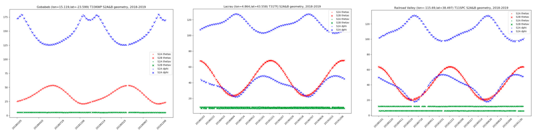
2.2. In-situ Surface Reflectances from the RadCalNet Network

RadCalNet dataset provides in-situ surface reflectances at nadir over a spectral range from 400 nm to 1000 nm (and up to 2500 nm, depending on each site’s instrumentation) at 10 nm spectral resolution [11]. These datasets are used intensively for satellite sensor validation [18]. Three RadCalNet sites are used in this study: the La Crau site in France, the Gobabeb site in Namibia and the Railroad Valley site in the US. The La Crau site shows moderate vegetation (grass) during winter and spring, while it tends towards semi-arid soil surfaces in summer. Gobabeb and Railroad Valley are typical flat deserts, bright targets homogeneous in time. RadCalNet in-situ measurements are derived from a Cimel CE-T312 photometer at La Crau and Gobabeb that can target either the sky or the surface to derive the atmospheric components and the surface BRDF [11]. At Railroad Valley, a ground-viewing radiometer (GVRs) with 8 bands is used [19]. The surface reflectances for the RadCalNet sites are normalized for nadir view using the estimated local BRDF model derived with the in-situ data.

Figure 1 shows the geometry of acquisitions for the S2 A&B over the three RadCalNet sites studied. In Figure 1, thetas is the sun zenith angle, thetav is the viewing angle and dphi is the relative azimuth angle (see [20] for the definition of the angles). At Gobabeb and La Crau, the S2 A&B viewing angles are low, with a maximum of 4° and 7.5° respectively (Figure 1, in green), making the normalization process less important than for other sensors with larger viewing angles.

At Railroad Valley, the viewing angle reaches 11.4° for the orbit 127. Among the in-situ data available from RadCalNet, we use the normalized (nadir viewing) surface reflectance ${\rho }_{situN}$(λ), the Aerosol Optical Thicknesses at 550 nm ($\mathrm{AOT}{550}_{situ})$ and the surface pressure.

2.3. BRDF Models and Reflectance Normalization

The normalization of the surface reflectances requires the use of a BRDF model describing the surface reflectance anisotropy. It is now commonly admitted that the BRDF can be represented with good accuracy by using a kernel-based semi-empirical model, which describes the reflectance as a sum of three angular kernels, Ki, weighted by the coefficients Fi:

$$\mathrm{BRDF}\left({\theta }_s,{\theta }_v,\mathsf{\Delta }\phi ,\lambda \right)\left(s{r}^{-1}\right)=\frac{Lu}{Ed}={\displaystyle \sum }_{k=0}^2{F}_k\left(\lambda \right)\ast K_k\left({\theta }_s,{\theta }_v,d\phi \right)$$

(2)

In Equation (2). ${\theta }_s,{\theta }_v,\mathsf{\Delta }\phi$ are, respectively, the sun, the view and the relative azimuth angles. $\lambda$ is the wavelength. Lu is the upward directional radiance and Ed the irradiance, i.e., the angular integration of the downward luminance Ld over the downward hemisphere (in the case, as for Sen2Cor, of a plan parallel atmosphere model [21]).

For this study, we use the initial BRDF model of Roujean et al. (2002) and the current RossTick-LiSparse (Ross-Li) model used by NASA [22] and [9]. In Equation (2), F0 represents the isotropic part of the reflectance, F1 mimics the contribution of the geometrical effects and F2 stands for the contribution of multiple scatterings.

Nadir-Normalized S2 Reflectances

Normalized reflectances are computed using the estimated BRDF to virtually replace the sensor at nadir. The nadir-normalized reflectances are then directly comparable with the RadCalNet nadir reflectance measurements. The goal of such normalization is also to favour inter-comparisons within and between the satellite time-series that are acquired within different geometric conditions. Finally, with these BRDF parameters, we apply the following equation to derive the nadir-normalized reflectances [23,24].

$${\rho }_N\left(\lambda \right)=\rho \left(\lambda ,{\theta }_s,{\theta }_v,\Delta \phi \right){\frac{BRDF\left({\theta }_s={\theta }_s, {\theta }_v=0, \Delta {\phi }_{}=0\right)}{BRDF\left({\theta }_s, {\theta }_v, \Delta {\phi }_{}\right)}}_{}$$

(3)

2.4. BRDF Parameter Estimation Using the Kalman Filter

The Kalman Filter (KF) is a recursive two-step algorithm that provides an estimate, at each time step n, of a state variable, Xn, of a system. It has been designed primarily to monitor processes for which it is crucial to accurately estimate the state of the system in the presence of noisy observations. In the KF, the estimation of the state variable X at time step n − 1 is first propagated in time by a linear temporal state-transition model, namely, the operator F, to obtain the a priori estimate $X_n^a$ for time step n:

$$X_n^a=F.X_{n-1}$$

(4)

The state vector covariance matrix C, representing the uncertainty on X, is propagated using the equation:

$$C_n^a=F.C_{n-1}.F_T+Q$$

(5)

Q stands for the model noise variance, i.e., the uncertainty of the model compared to the real physical process.

In a second step, measurements (here, the surface reflectances) Z are related to the state variable by the linear relationship $Z=H.X+v,$ where H is the observation model (matrix), and v a random white noise of variance R describing the measurement noise. The state vector estimate and covariance are then corrected using:

$$X_n^{}=X_n^a+G_n\left(Z_n-H.X_n^a\right);C_n^{}=\left(1-G_n.H_n^{}\right).C_n^a$$

(6)

where $G_n$ is the Kalman gain expressed as:

$$G_n=C_n^a{H}^T{\left(H{C}_n^a{H}_T+R\right)}^{-1}$$

(7)

The Kalman gain is thus a function of the state vector covariance and the measurement noise. In the present study, the state vector $X$ is the set of parameters of the BRDF model, i.e., [k0, k1, k2]. The observation matrix for the reflectance is then simply written as H = [1 f 1 f 2 ].

2.4.1. Outlier Removals

One may use the first step of the Kalman filtering to verify if an observation Z, newly acquired at dt, the time step between the new and the latest observation, follows the KF hypothesis. The advantage of the KF, compared to a simple linear regression, is the possibility of detecting the outliers, given the a priori knowledge of the a priori state vector. To ensure the KF hypothesis, the new observation Z must ensure:

$${\left|Z-H.X_n^a\right|}^2\le 4\ast diag\left(R+H.C_n^a.H^T\right)$$

(8)

2.4.2. Temporal Model

Temporal model of the model noise variance matrix Q is proportional to the state vector, with the off-diagonal elements set to zero. We introduced some variance regarding dt, as the more the gap between the observations increases, the less the latest estimation of X is relevant:

$$diag\left(Q\right)=\left|X_{n-1}^{}\right|{10}^{-3}-{10}^{-4}\ast \mathrm{dt}$$

(9)

2.4.3. Observation Uncertainties

Observation uncertainty covariance matrix ${\mathrm{R}}_i$ for observation i is set to be proportional to the reflectance level:

$${\mathrm{R}}_i\left(\lambda \right)={\left(0.05{\rho }_i\left(\lambda \right)+R_0\right)}^2$$

(10)

where $R_0$ is set to 3% of the standard deviation of $\rho \left(\lambda \right)$, the surface reflectance.

2.5. BRDF Parameter Estimation Using the Standard Weighted Linear Inversion

The results obtained with the KF are compared to the method used by NASA and MODIS [9], i.e., a standard least square, optimized here using a Bounded Variable Least Squares (BVLS) regression analysis to avoid geophysically meaningless estimates. The method consists of inverting the Equation (2) with the data collected over a sliding temporal window of 30 days. To favor those observations which are temporally close to the studied date, a temporal weighting is performed to give more importance to the data close to the window’s center [9].

2.6. Aerosol and Rayleigh Corrected Sen2Cor Reflectances

The angular kernels K are, by definition, very sensitive to the geometry. In order to unmix the errors performed by the atmospheric corrections from the BRDF estimation & the reflectance normalization, and before the BRDF estimation, we apply an aerosol and Rayleigh correction, given the aerosol loads and the surface pressure measured at the RadCalNet stations. We next use the libRadtran libraries to correct the Sen2Cor estimates, given the in-situ observations. With ${\rho }_{path}$ being the aerosol and Rayleigh reflectances (including the coupling term [25] between the Rayleigh and aerosols), the error $E{\rho }_{path}$ is estimated using:

$$\mathit{E}{\mathit{\rho }}_{\mathit{p}\mathit{a}\mathit{t}\mathit{h}=} {\mathit{\rho }}_{\mathit{p}\mathit{a}\mathit{t}{\mathit{h}}_{\mathit{S}\mathbf{2}\mathit{C}}}-{\mathit{\rho }}_{\mathit{p}\mathit{a}\mathit{t}\mathit{h}\_\mathit{s}\mathit{i}\mathit{t}\mathit{u}}$$

(11)

and the transmittance error is estimated using:

$$\mathit{E}\mathit{T}{\mathit{d}}_{\mathit{p}\mathit{a}\mathit{t}\mathit{h}=} \mathit{T}{\mathit{d}}_{\mathit{p}\mathit{a}\mathit{t}{\mathit{h}}_{\mathit{S}\mathbf{2}\mathit{C}}}/\mathit{T}{\mathit{d}}_{\mathit{p}\mathit{a}\mathit{t}\mathit{h}\_\mathit{s}\mathit{i}\mathit{t}\mathit{u}}$$

(12)

In the equation above, ${\rho }_{pat{h}_{S2C}}$ (and respectively $T{d}_{pat{h}_{S2C}})$ is the path reflectance estimated using the AOT, aerosol model and surface pressure used by Sen2Cor, while $E{\rho }_{pat{h}_{situ}}$ is the path reflectance estimated using the measurements at the RadCalNet stations.

Finally, the corrected Sen2Cor surface reflectances are estimated using Equation (1):

$${\mathit{\rho }}^{*}\left(\mathit{\lambda }\right)=\mathit{\rho }\left(\mathit{\lambda }\right)*\mathit{E}\mathit{T}{\mathit{d}}_{\mathit{p}\mathit{a}\mathit{t}\mathit{h}}+\frac{\mathit{E}{\mathit{\rho }}_{\mathit{p}\mathit{a}\mathit{t}\mathit{h} }}{\mathit{T}{\mathit{d}}_{\mathit{p}\mathit{a}\mathit{t}\mathit{h}\_\mathit{s}\mathit{i}\mathit{t}\mathit{u}}}$$

(13)

It must be noted that this preliminary correction is not mandatory for BRDF estimation and reflectance normalization. Nevertheless, the normalized reflectances after this step showed better results compared with the in-situ data, exhibiting the importance of this correction.

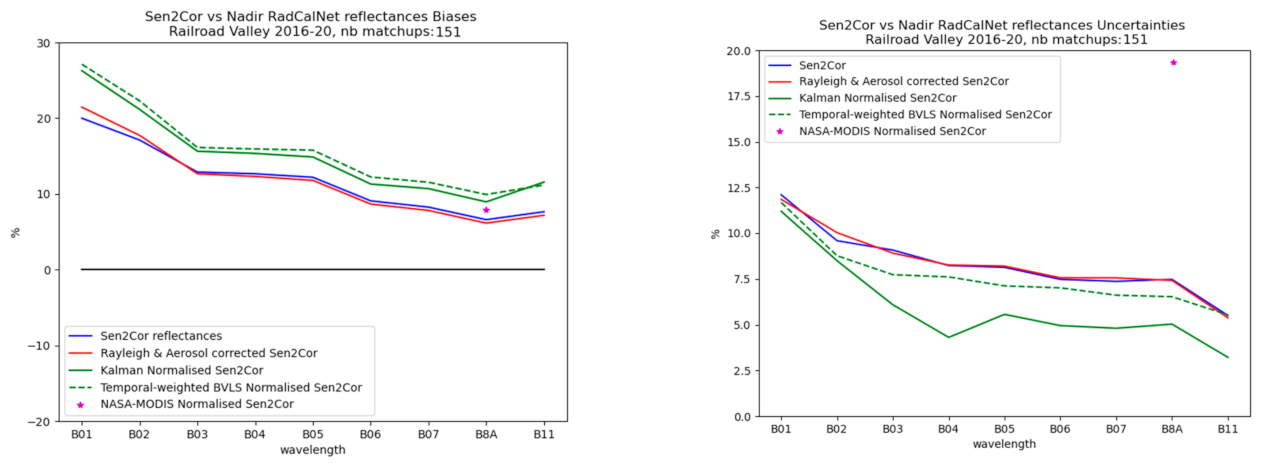
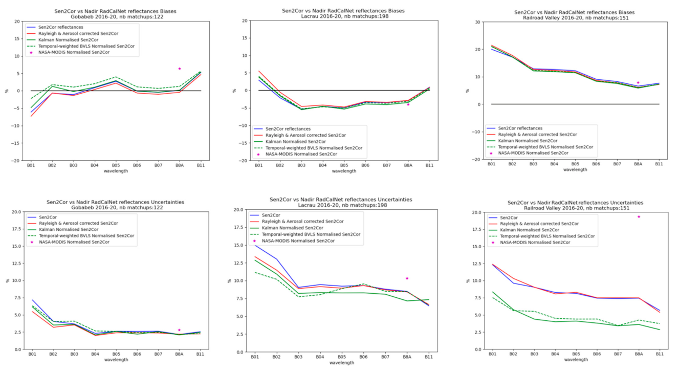
2.7. Statistical Diagnostics

Qualification of the results is performed using accuracy A and uncertainties U of the estimated normalized reflectances:

$$\mathrm{A}\left(\widehat{{\rho }^{*}}\left(\lambda \right)\right)=\frac{1}{\mathrm{n}}\sum \left(\widehat{{\rho }^{*}}\left(\lambda \right)-{\rho }^{*}\left(\lambda \right)\right)$$

(14)

and

$$\mathrm{U}\left(\widehat{{\rho }^{*}}\left(\lambda \right)\right)=\sqrt{\frac{1}{\mathrm{n}}\sum {\left(\widehat{{\rho }^{*}}\left(\lambda \right)-{\rho }^{*}\left(\lambda \right)\right)}^2}$$

(15)

3. Results

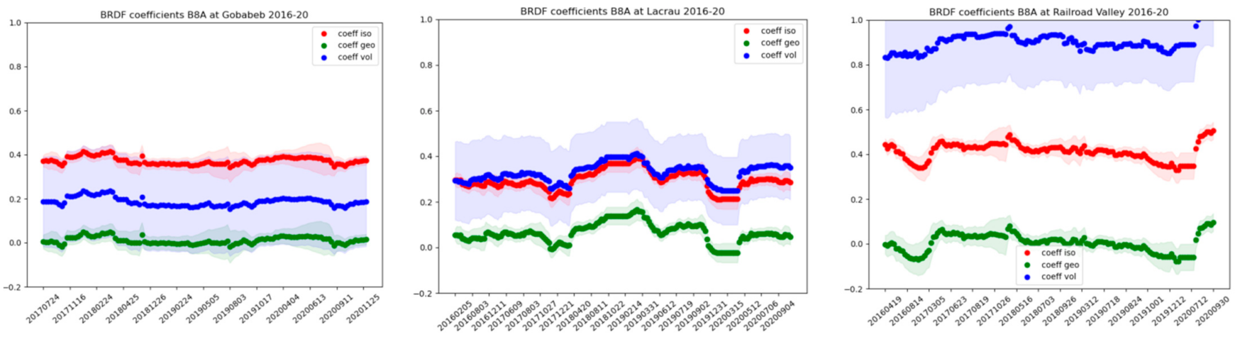
3.1. Estimated BRDF Coefficients

Figure 2 shows the estimated BRDF coefficients at the three RadCalNet stations using the KF and the Roujean Kernels. At Gobabeb, the coefficients are constants in time, while, at La Crau, some seasonal cycles appear. The magnitude and the uncertainties of the estimated coefficients are comparable to those obtained by Samain and Roujean [26] for Bare Lands (Gobabeb-like) and semi-arid open lands, using a similar approach and the SPOT-4 vegetation instrument. At Railroad Valley, a possible scenario to explain the increase in the volume scattering coefficient is an increase in the surface roughness due to a recrudescence of dusts [24].

3.2. Normalized Sen2cor Surface Reflectances Using the Roujean Kernels

In Figure 3 the normalization results are shown in accuracy (biases) and uncertainties for the three RadCalNet sites. At Gobabeb the normalization process tends to minimize the bias. The KF approach shows less bias than the classical linear inversion with the temporal weighting. Uncertainty reductions at Gobabeb are very low because of the very low viewing angle (<4.5°) and the isotropic behavior of the surface (Figure 2).

At La Crau, the aerosol and the Rayleigh correction introduce a minimal bias of 2% for B01 and B02, but they reduce the uncertainties at these bands. At La Crau, the KF reduces uncertainties more than the classical linear inversion, with a mean reduction of 2% for all considered bands.

At Railroad Valley, the initial Sen2Cor products show positive biases from 10 to 20%, depending on the bands. Aerosol and Rayleigh corrections do not correct the observed biases (Figure 3, right). The KF normalization diminishes the uncertainties by 5%, which is the larger of the reductions observed among the three sites. This important improvement in the time series may be due to the fact that the viewing angle for orbit 127 is larger at Railroad Valley, and the surface here is more anisotropic compared with Gobabeb (Figure 2).

The red stars in Figure 3 show the normalization results obtained using the MODIS BRDF MCD43A1 (500 m resolution) BRDF parameters for the MODIS band 2, spectrally close to the S2 B08, applied using the Ross-Li kernels and Equation (3). S2-normalized reflectances at Gobabeb using these coefficients show some slight positive biases of 5% and are in agreement with our estimates at La Crau and Railroad Valley. The results for uncertainties are worse when compared with our approach, with some uncertainty levels of 3, 11 and 19%, respectively, for Gobabeb, La Crau and Railroad Valley. These results show that our approach performs better for the S2 B08 than the direct application of the MODIS-estimated BRDF parameters.

3.3. Normalized Sen2cor Surface Reflectances Using the Ross-Li Kernels at Railroad Valley

In Figure 4, the normalization results using the Ross-Li Kernels for the Railroad Valley site are shown. Both the weighted linear inversion and the KF introduce some positive biases, and the KF approach shows lower bias than the classical weighted linear inversion. With the exception of B01, uncertainty reductions are larger using the KF filtering compared to the weighted linear inversion. Note that, for the La Crau and Gobabeb sites, the results (not shown) also clearly showed lower performances compared with the Roujean kernels.

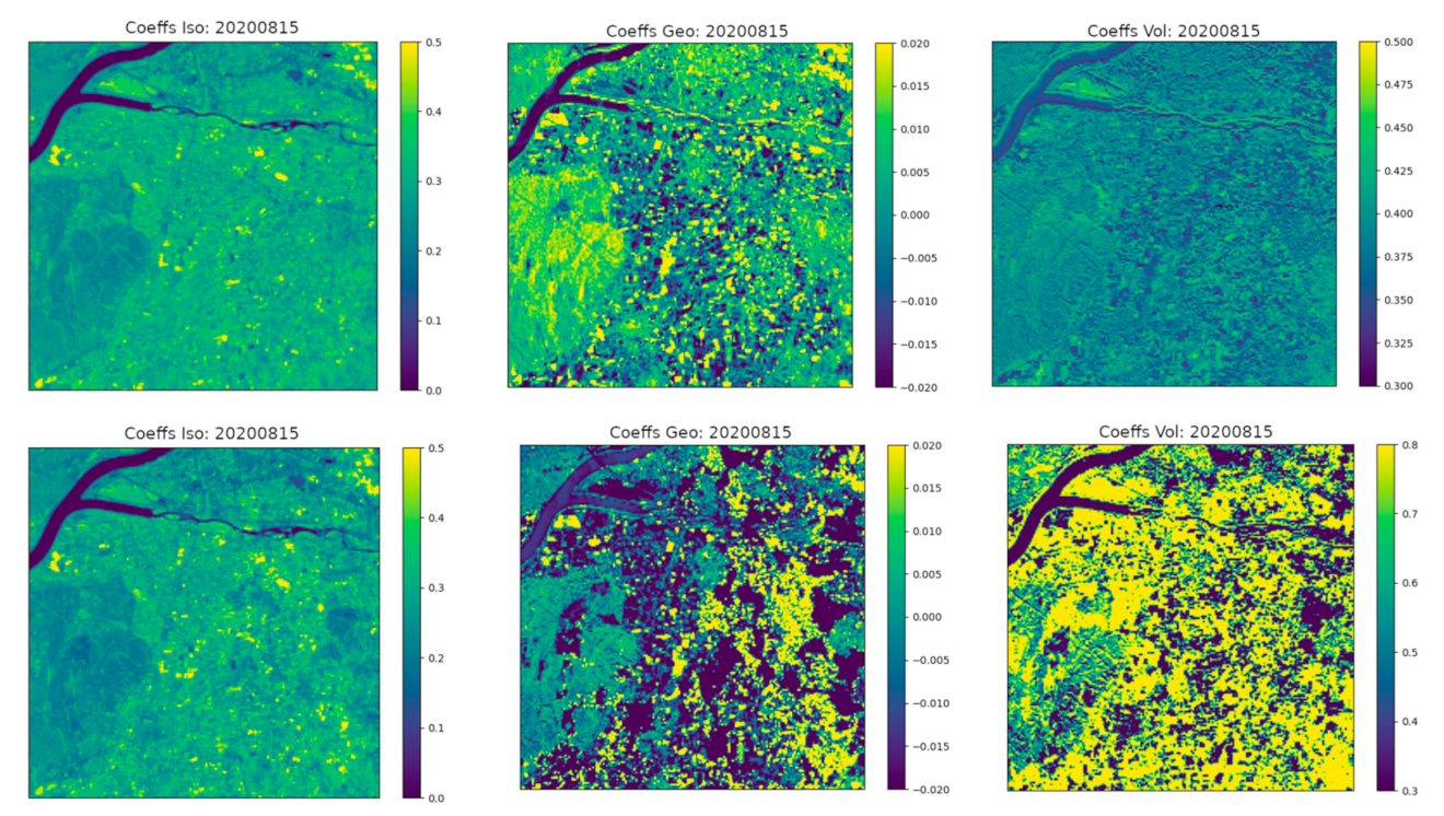
3.4. Spatial Distribution of the Estimated BRDF Coefficients for La Crau and B8A

Figure 5 shows the estimated coefficients at La Crau for the 20200815 using four images: 20200731, 20200805, 20200807 and 20200815. While the isotropic coefficients are comparable for the KF and the weighted linear inversion (Figure 5, left) it is clear that the geometric and the volume scattering coefficients estimated using the KF are spatially smoother. The linear inversion, even if bounded or constrained (BVLS, [27]), shows spatial discontinuities in the estimations. This is caused by the high sensitivity of the used BRDF model to the noise in the observations. This topic is particularly well addressed by the Kalman filtering approach.

4. Discussion

To our knowledge, this study is the first to normalize S2 Sen2cor reflectances using a Kalman filtering approach. Here, we show that the BRDF models used are very sensitive to the noise measurements. The atmospheric correction process performed to retrieve the surface reflectances, used as input of the BRDF estimation, introduces itself some noise. The use of the Kalman filtering, robust to the noise, allows for the retrieval of more consistent and reliable BRDF parameters. Conversely, the use of a classical linear inversion (OLS, or constrained-bounded version BVLS) often leads to spatial and temporal discontinuities in the estimated geometric and volume-scattering coefficients. These inversion issues were more visible when looking at the estimated BRDF coefficients. In the case of a classical linear inversion being used, the BRDF coefficients may not have any geophysical reality. These issues may not appear while checking only the differences between the estimated normalized reflectances and the RadCalNet data. This is caused by i/ non-homogeneous BRDF coefficients in time and space, which may lead to reliable normalized reflectances and ii/ the close to nadir position of the S2 sensors with, most of the times, a viewing angle lower than 10°. In the case of S2, the simulation of the nadir position of the sensor is by definition often close to the non-normalized estimates.

In any case, the KF approach showed better results in terms of the biases and uncertainties than the classical weighted linear inversion at the three selected RadCalNet sites of Gobabeb, La Crau and Railroad Valley. Regarding the BRDF kernels that were used, the Roujean kernels performed better than the Ross-Li kernels at the RadCalNet sites. This might be caused by the difference in definition of the volume scattering coefficients between the two models. For other types of surfaces (typically forests) that are not addressed by the RadCalNet sites studied here, these results may change.

Compared with the direct use of the MODIS MCD43A1 (500 m resolution) BRDF parameters, normalization results for bands B08 showed great improvements using the Kalman filtering approach, especially for uncertainties. This stresses the need to estimate dedicated BRDF parameters using the S2 data.

Further improvements to the approach may involve more complex temporal models for the Kalman filtering, introducing, for example, some external classifications. The proposed approach provides currently potential improvements for S2 and the possibility of delivering reliable BRDF coefficients at global scale. The provision of daily global maps of land surface BRDF coefficients and the derived normalized S2 reflectances with such an approach will be extremely useful to the global and regional climate modelling communities and the world cover monitoring. It also allows for potential improvements for other current surface albedo products, either those derived from the geostationary MSG (Meteosat Second Generation) or the sun-synchronous S3 (Sentinel 3), Landsat (Land Remote-Sensing Satellite), MODIS and PACE (Plankton, Aerosol, Cloud, ocean Ecosystem) missions. The approach can also be applied to other related biophysical variables such as the Leaf Area Index (LAI), the fraction of vegetation cover and the fraction of Absorbed Photosynthetically Active Radiation (FAPAR). The proposed work also contributes to the future use of assimilation techniques, typically ECMWF (European Centre for Medium-Range Weather Forecasts) products, to enhance the satellite-derived estimates. In a larger vision, any inversion using satellite reflectance observations could take advantage of the KF approach proposed here, including the atmospheric correction itself. In the case of the atmospheric correction that relies on non-linear functions, the Extended Kalman Filter will have to be used [28].

Thus, the implementation of the KF technique in the official processing chains would participate constructively with the European Space Agency’s (ESA) Calibration/Validation Strategy to create continuous time series and increase the inter-sensor’s interoperability in the optical domain [29].

References

1. Drusch, M.; Del Bello, U.; Carlier, S.; Colin, O.; Fernandez, V.; Gascon, F.; Bargellini, P. Sentinel-2: ESA’s optical high-resolution mission for GMES operational services. Remote Sens. Environ. 2012, 120, 25–36. [Google Scholar] [CrossRef]
2. Copernicus Sentinel Data Access Annual Report 2019. Available online: https://sentinels.copernicus.eu/web/sentinel/news/-/asset_publisher/xR9e/content/copernicus-sentinel-data-access-annual-report-2019;jsessionid=4DC08B0ABC1B60CB9A889CD1AF2B53B1.jvm2?redirect=https%3A%2F%2Fsentinels.copernicus.eu%2Fweb%2Fsentinel%2Fnews%3Bjsessionid%3D4DC08B0ABC1B60CB9A889CD1AF2B53B1.jvm2%3Fp_p_id%3D101_INSTANCE_xR9e%26p_p_lifecycle%3D0%26p_p_state%3Dnormal%26p_p_mode%3Dview%26p_p_col_id%3Dcolumn-1%26p_p_col_count%3D1%26_101_INSTANCE_xR9e_keywords%3D%26_101_INSTANCE_xR9e_advancedSearch%3Dfalse%26_101_INSTANCE_xR9e_delta%3D20%26_101_INSTANCE_xR9e_andOperator%3Dtrue (accessed on 28 June 2021).
3. S2MPC Team. Sentinel-2 Data Quality Report; Tech. Rep. S2-PDGS-MPC-DQR; 2021; Available online: https://sentinels.copernicus.eu/documents/247904/685211/Sentinel-2_L1C_Data_Quality_Report.pdf/6ad66f15-48ca-4e65-b304-59ef00b7f0e0?t=1628261039520 (accessed on 28 June 2021).
4. Thorne, P.W.; Diamond, H.J.; Goodison, B.; Harrigan, S.; Hausfather, Z.; Ingleby, N.B.; Jones, P.D.; Lawrimore, J.H.; Lister, D.H.; Merlone, A.; et al. Towards a global land surface climate fiducial reference measurements network. Int. J. Climatol. 2018, 38, 2760–2774. [Google Scholar] [CrossRef]
5. Level-2A Algorithm Theoretical Basis Document. 2011. Available online: https://earth.esa.int/c/document_library/get_file?folderId=349490&name=DLFE-4518.pdf (accessed on 28 June 2021).
6. Lewis, A.; Lacey, J.; Mecklenburg, S.; Ross, J.; Siqueira, A.; Killough, B.; Szantoi, Z.; Tadono, T.; Rosenavist, A.; Goryl, P.; et al. CEOS analysis ready data for Land (CARD4L) overview. In Proceedings of the IGARSS 2018—2018 IEEE International Geoscience and Remote Sensing Symposium, Valencia, Spain, 22–27 July 2018; pp. 7407–7410. [Google Scholar]
7. Talagrand, O. Assimilation of observations, an introduction (gtspecial issueltdata assimilation in meteology and oceanography: Theory and practice). J. Meteorol. Soc. Jpn. 1997, 75, 191–209. [Google Scholar] [CrossRef] [Green Version]
8. Kalman, R.E. A New Approach to Linear Filtering and Prediction Problems. Trans. ASME J. Basic Eng. 1960, 35–45. [Google Scholar] [CrossRef] [Green Version]
9. Strahler, A.H.; Muller, J.; Schaaf, C.B.; Hu, B.; Muller, J.P.; Lewis, P.; Barnsley, M.J. MODIS BRDF/albedo product: Algorithm theoretical basis document version 5.0. MODIS Doc. 1999, 23, 42–47. [Google Scholar]
10. Justice, C.O.; Townshend, J.R.G.; Vermote, E.F.; Masuoka, E.; Wolfe, R.E.; Saleous, N.; Roya, D.P.; Morisette, J.T. An overview of MODIS Land data processing and product status. Remote Sens. Environ. 2002, 83, 3–15. [Google Scholar] [CrossRef]
11. Bouvet, M.; Thome, K.; Berthelot, B.; Bialek, A.; Czapla-Myers, J.; Fox, N.P.; Goryl, P.; Henry, P.; Ma, L.; Marcq, S.; et al. RadCalNet: A radiometric calibration network for Earth observing imagers operating in the visible to shortwave infrared spectral range. Remote Sens. 2019, 11, 2401. [Google Scholar] [CrossRef] [Green Version]
12. Louis, J.; Pflug, B.; Main-Knorn, M.; Debaecker, V.; Mueller-Wilm, U.; Iannone, R.Q.; Cadau, E.H.; Boccia, V.; Gascon, F. Sentinel-2 global surface reflectance level-2A product generated with Sen2Cor. In Proceedings of the IGARSS 2019—2019 IEEE International Geoscience and Remote Sensing Symposium, Yokohama, Japan, 28 July–2 August 2019; pp. 8522–8525. [Google Scholar]
13. Saulquin, B.; Fablet, R.; Bourg, L.; Mercier, G.; d’Andon, O.F. MEETC2: Ocean color atmospheric corrections in coastal complex waters using a Bayesian latent class model and potential for the incoming sentinel 3—OLCI mission. Remote Sens. Environ. 2016, 172, 39–49. [Google Scholar] [CrossRef] [Green Version]
14. Mayer, B.; Kylling, A. Technical note: The libRadtran software package for radiative transfer calculations—Description and examples of use. Atmos. Chem. Phys. 2005, 5, 1855–1877. [Google Scholar] [CrossRef] [Green Version]
15. Kaufman, Y.J.; Remer, L.A. Detection of forests using mid-IR reflectance: An application for aerosol studies. IEEE Trans. Geosci. Remote Sens. 1994, 32, 672–683. [Google Scholar] [CrossRef]
16. Hu, B.; Lucht, W.; Strahler, A.H. The interrelationship of atmospheric correction of reflectances and surface BRDF retrieval: A sensitivity study. IEEE Trans. Geosci. Remote Sens. 1999, 37, 724–738. [Google Scholar]
17. Van Zyl, J.J. The Shuttle Radar Topography Mission (SRTM): A breakthrough in remote sensing of topography. Acta Astronaut. 2001, 48, 559–565. [Google Scholar] [CrossRef]
18. Banks, A.C.; Hunt, S.E.; Gorroño, J.; Scanlon, T.; Woolliams, E.R.; Fox, N.P. A comparison of validation and vicarious calibration of high and medium resolution satellite-borne sensors using RadCalNet. In Proceedings of the Sensors, Systems, and Next-Generation Satellites XXI, Warsaw, Poland, 11–14 September 2017; Volume 10423, p. 104231A. [Google Scholar]
19. Anderson, N.J.; Czapla-Myers, J.S. Ground viewing radiometer characterization, implementation and calibration applications: A summary after two years of field deployment. In Earth Observing Systems XVIII; International Society for Optics and Photonics: Bellingham, WA, USA, 2013; Volume 8866, p. 88660N. [Google Scholar] [CrossRef]
20. Vescovi, F.D.; Lankester, T.; Coleman, E.; Ottavianelli, G. Harmonisation initiatives of Copernicus data quality control. Int. Arch. Photogramm. Remote Sens. Spat. Inf. Sci. 2015, 40, 713. [Google Scholar] [CrossRef] [Green Version]
21. Lenoble, J. (Ed.) Radiative Transfer in Scattering and Absorbing Atmospheres: Standard Computational Procedures; A Deepak: Hampton, VA, USA, 1985; Volume 300. [Google Scholar]
22. Ross, J. The Radiation Regime and Architecture of Plant Stands; Springer: Norwell, MA, USA, 1981; Volume 392, p. 1981. [Google Scholar]
23. Franch, B.; Vermote, E.; Skakun, S.; Roger, J.-C.; Masek, J.; Ju, J.; Villaescusa-Nadal, J.L.; Santamaria-Artigas, A. A method for Landsat and Sentinel 2 (HLS) BRDF normalization. Remote Sens. 2019, 11, 632. [Google Scholar] [CrossRef] [Green Version]
24. Lyapustin, A.I.; Wang, Y.; Laszlo, I.; Hilker, T.; Hall, F.G.; Sellers, P.J.; Tuckera, C.J.; Korkin, S.V. Multi-angle implementation of atmospheric correction for MODIS (MAIAC): 3. Atmospheric correction. Remote Sens. Environ. 2012, 127, 385–393. [Google Scholar] [CrossRef]
25. Vermote, E.F.; Tanré, D.; Deuze, J.L.; Herman, M.; Morcette, J.J. Second simulation of the satellite signal in the solar spectrum, 6S: An overview. IEEE Trans. Geosci. Remote Sens. 1997, 35, 675–686. [Google Scholar] [CrossRef] [Green Version]
26. Samain, O.; Roujean, J.L.; Geiger, B. Use of a Kalman filter for the retrieval of surface BRDF coefficients with a time-evolving model based on the ECOCLIMAP land cover classification. Remote Sens. Environ. 2008, 112, 1337–1346. [Google Scholar] [CrossRef]
27. Stark, P.B.; Parker, R.L. Bounded-variable least-squares: An algorithm and applications. Comput. Stat. 1995, 10, 129–142. [Google Scholar]
28. Einicke, G.A.; White, L.B. Robust extended Kalman filtering. IEEE Trans. Signal Process. 1999, 47, 2596–2599. [Google Scholar] [CrossRef]
29. Niro, F.; Goryl, P.; Dransfeld, S.; Boccia, V.; Gascon, F.; Adams, J.; Themann, B.; Scifoni, S.; Doxani, G. European Space Agency (ESA) Calibration/Validation Strategy for Optical Land-Imaging Satellites and Pathway towards Interoperability. Remote Sens. 2021, 13, 3003. [Google Scholar] [CrossRef]
Figure 1. Geometry of acquisition for the S2A&B at the three selected RadCalNet sites. Left, Gobabeb is observed only on the orbit 107. Middle, La Crau is observed on both orbits 8 and 108. Right, Railroad Valley is observed on orbits 27 and 127.
Remotesensing 13 03373 g001
Figure 2. Time series of BRDF cefficients using the Roujean Kernels and the Kalman filtering approach, and related uncertainties for each parameter.
Remotesensing 13 03373 g002
Figure 3. Statistical assessment of normalized Sen2Cor reflectances vs. in-situ data using the Roujean Kernels. Top, accuracy (biases) and bottom, uncertainties. The red stars correspond to the normalization results obtained using directly the MODIS band 2 BRDF MCD43A1 (500 m resolution) parameters and the related Ross-Li kernels.
Remotesensing 13 03373 g003
Figure 4. Statistical assessment of normalized Sen2Cor reflectances vs. in-situ data using the Ross-Li kernels at Railroad Valley. Left, accuracy (biases) and right, uncertainties. The red stars correspond to the normalization results obtained using directly the MODIS band 2 BRDF MCD43A1 (500 m res.) parameters and the related Ross-Li kernels.
Remotesensing 13 03373 g004
Figure 5. BRDF coefficients k0 (isotropic, top), k1 (geometric, middle) and k2 (volume scattering, right) at La Crau for the S2 B8A image of the 20200815 obtained using the Kalman filter (top) and the classical weighted linear inversion (bottom).
Remotesensing 13 03373 g005
Publisher’s Note: MDPI stays neutral with regard to jurisdictional claims in published maps and institutional affiliations.