Article

Carbon Stocks, Species Diversity and Their Spatial Relationships in the Yucatán Peninsula, Mexico

by
José Luis Hernández-Stefanoni
1,*,
Miguel Ángel Castillo-Santiago
2,
Juan Andres-Mauricio
1,
Carlos A. Portillo-Quintero
3,
Fernando Tun-Dzul
1 and
Juan Manuel Dupuy
1
1
Centro de Investigación Científica de Yucatán A.C., Unidad de Recursos Naturales, Calle 43 # 130, Colonia Chuburná de Hidalgo, Mérida CP 97200, Mexico
2
Laboratorio de Análisis de Información Geográfica y Estadística, El Colegio de la Frontera Sur, Carretera Panamericana y Periférico sur s/n., San Cristóbal de las Casas, Chiapas CP 29290, Mexico
3
Geospatial Technologies Laboratory, Department of Natural Resources Management, Texas Tech University, Box 42125, Lubbock, TX 79409-2125, USA
*
Author to whom correspondence should be addressed.
Remote Sens. 2021, 13(16), 3179; https://doi.org/10.3390/rs13163179
Submission received: 14 June 2021 / Revised: 5 August 2021 / Accepted: 9 August 2021 / Published: 11 August 2021

Abstract

:
Integrating information about the spatial distribution of carbon stocks and species diversity in tropical forests over large areas is fundamental for climate change mitigation and biodiversity conservation. In this study, spatial models showing the distribution of carbon stocks and the number of species were produced in order to identify areas that maximize carbon storage and biodiversity in the tropical forests of the Yucatan Peninsula, Mexico. We mapped carbon density and species richness of trees using L-band radar backscatter data as well as radar texture metrics, climatic and field data with the random forest regression algorithm. We reduced sources of errors in plot data of the national forest inventory by using correction factors to account for carbon stocks of small trees (<7.5 cm DBH) and for the temporal difference between field data collection and imagery acquisition. We created bivariate maps to assess the spatial relationship between carbon stocks and diversity. Model validation of the regional maps obtained herein using an independent data set of plots resulted in a coefficient of determination (R2) of 0.28 and 0.31 and a relative mean square error of 38.5% and 33.0% for aboveground biomass and species richness, respectively, at pixel level. Estimates of carbon density were influenced mostly by radar backscatter and climatic data, while those of species richness were influenced mostly by radar texture and climatic variables. Correlation between carbon density and species richness was positive in 79.3% of the peninsula, while bivariate maps showed that 39.6% of the area in the peninsula had high carbon stocks and species richness. Our results highlight the importance of combining carbon and diversity maps to identify areas that are critical—both for maintaining carbon stocks and for conserving biodiversity.

Graphical Abstract

1. Introduction

Tropical forests are one of the most important reservoirs of carbon in the world, representing approximately 25% of the above and belowground terrestrial carbon stock [1]. In turn, tropical dry forests (TDF) represent more than 18% of the carbon stocks in the tropics [2] and are one of the most important tropical ecosystems, covering more than 40% of tropical forest regions in the world and 54% of the tropical forest in the Neotropics [3]. At the same time, tropical forests harbor more than 96% of all tree species estimated in all ecosystems worldwide [4]. TDF have lower levels of species diversity than humid tropical forests but have high levels of endemic plant species [5]. Unfortunately, deforestation is one of the greatest threats to these forests and is a significant source of greenhouse emissions aggravating global climate change [6]. Forest conversion also impacts plant diversity [7]. Therefore, integrating information about the spatial distribution of carbon stocks and plant species diversity of tropical forests over large areas is fundamental for climate change mitigation and biodiversity conservation.
Several studies have mapped the spatial distribution of carbon density, aboveground biomass (AGB) or species richness of plants at continental or global scales [8,9,10,11]. These maps have been elaborated with low spatial resolutions of 1 km or more. Other weaknesses of these studies have included a suboptimal number and distribution of sampling field plots over the area covered with remotely sensed data, as well as the use of field plots with different sizes, which make calibration and validation of the models more challenging [12,13]. Other studies have produced maps of carbon density or AGB at national or regional scales with finer spatial resolutions, close to 30 m [14,15]. These maps used mainly field data obtained from national forest inventories (NFI), which provide a more representative number of sampling plots as well as detailed information of vegetation structure used to estimate biomass [16]. In contrast, despite the current alarming loss of biodiversity, there is a lack of plant diversity maps with high spatial resolution at regional scales [17]. In this work, we created one of the first regional maps of tree species diversity with high spatial resolution (25 m) using the TDF of the Yucatan Peninsula as a model.
The Yucatan peninsula contains the second largest forest massif in the Americas (after the Amazon) and is dominated by different types of seasonal TDF with high levels of endemicity [18]. It is therefore important to estimate and map AGB or carbon density and plant diversity in this region. The TDFs of the Yucatan Peninsula comprise a large number of small-sized trees, which account for 15% to 40% of the biomass in mature TDFs and more than 80% of the biomass in young TDFs [19], and also contribute greatly to the species richness [20], especially in secondary forests [21]. However, the NFI in Mexico provides measurements only for trees with a diameter at breast height (DBH) above 7.5 cm [22]. Excluding small size trees from the NFI leads to a significant underestimation of AGB and species richness and requires the application of specific correction factors [23]. Additionally, the last Mexican NFI was conducted between 2009 and 2014; this six-year time interval resulted in temporal differences between field data collection and imagery acquisition, making it necessary to take into account changes in AGB due to growth, recruitment and mortality of trees. Using AGB as opposed to stand age functions obtained from chronosequence data can help to build predictive models of biomass changes over time that can be used to update field biomass estimates from NFI plots [23].
Studies estimating the spatial distribution of forest biomass and species richness through remotely sensed data have utilized different approaches and different remotely sensed data [24,25]. Biomass is generally influenced by vegetation structural attributes such as height of trees, stem diameter and basal area. Synthetic Aperture Radar (SAR) sensors are sensitive to forest structure, as backscatter signals are able to penetrate forest canopy. In particular, the Advanced Land Observing Satellite (ALOS) Phased Array L-band Synthetic Aperture Radar (PALSAR) from the Japanese Aerospace Exploration Agency (JAXA), with a wavelength of 23 cm, a pixel size of 25 m and full coverage over the world, provides data on forest structure that can be used to map carbon density or AGB at regional to global scales.
Variation in vegetation structure can also positively influence AGB; for example, leaf layering can improve light capturing, allowing plant communities to increase carbon storage [1]. Texture metrics of very high-resolution imagery have been successfully used to capture variation in the structure of tropical forests [26]. Even though the 25 m spatial resolution of ALOS-PALSAR imagery cannot discern individual trees or canopy openings, it can capture broader scales of variation, such as fragments with different successional age that differ in vegetation structure [27]. Thus, texture metrics from backscatter data can help to improve carbon density and AGB estimations while also allowing for reductions of the effects of saturation of radar backscatter signal [28].
Species diversity also increases with forest structure [17], but has been found to be strongly and positively associated with environmental or habitat heterogeneity [29], which is in turn associated with higher availability of niches [30]. There are different ways to measure environmental heterogeneity from remotely sensed data, from using variance of spectral data to more complex methods such as texture metrics, which reflect spatial variation within a moving window in an image [31]. Therefore, texture metrics derived from radar sensors can be used to estimate species diversity.
Additionally, at regional scales, several factors affect biomass and species richness including precipitation, soil fertility and time since disturbance. These factors are positively related to tropical tree species richness and forest biomass [32,33]. For seasonally dry forests, a measure of water deficit based on the difference between precipitation and evapotranspiration is particularly important as it affects rates of tree growth and recruitment [32]. Therefore, including water deficit may improve the accuracy of tree species richness and biomass maps in TDF.
Some studies have suggested a positive association between carbon density or AGB and species diversity. Forest biomass or carbon density has been used as a predictor of species richness, as plant diversity often shows a hump-shaped or saturating relationship with productivity [34]. Conversely, species diversity can foster biomass production through niche complementarity—that is, a more thorough and efficient use of resources by coexisting species due to a more complete occupation of available niches [35]. However, some studies have found weak or negative relationships between carbon density and species diversity [36]. The type of association between carbon density and diversity is of paramount importance, as areas that have both high carbon stocks and high levels of species diversity could provide climate change mitigation and biodiversity conservation at the same time. However, different strategies are required for areas of high diversity but low carbon stocks versus areas with low diversity and high carbon stocks.
Considering the importance of the relationship between carbon density and plant species diversity, the aims of this study were two-fold. First, we sought to improve the accuracy of regional maps of carbon density and tree species richness of the Yucatan peninsula by using L-band radar backscatter data, radar texture metrics, climatic and field data with the random forest regression algorithm. By accounting for carbon stocks and species richness of small trees, and for temporal differences between NFI field data collection and imagery acquisition, we expected to improve the accuracy of carbon density maps compared to previous studies. We also expected that the spatial distribution of carbon density would be more strongly related to radar backscatter (reflecting variation in forest structure), while species richness would be more strongly associated with texture metrics (reflecting structural heterogeneity). Second, we obtained bivariate maps of carbon density and tree species richness in order to evaluate the spatial relationships of these variables and to identify areas that maximize carbon storage and biodiversity in the tropical dry forests of Yucatan peninsula.

2. Materials and Methods
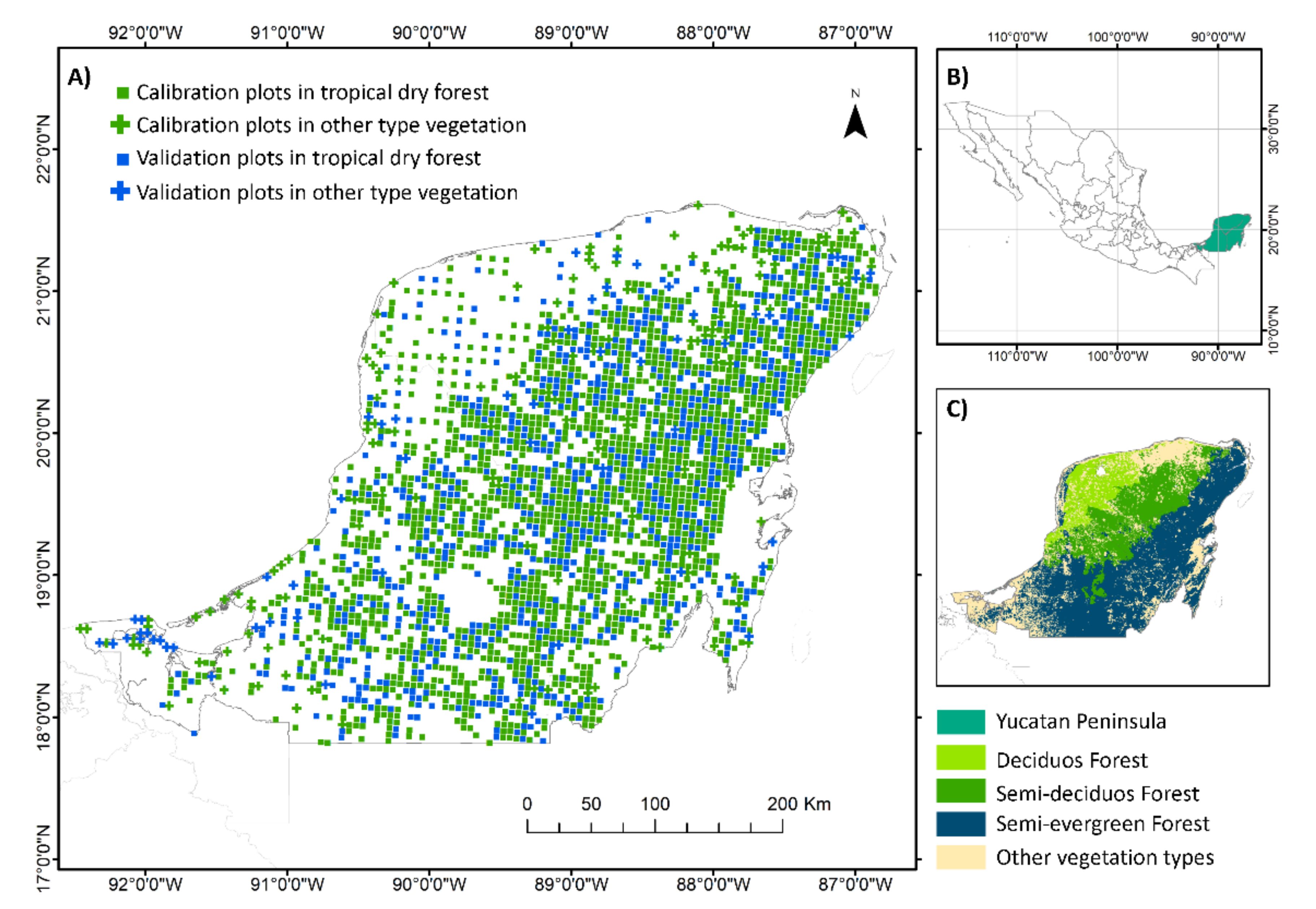
2.1. Study Area

This study focused on the Yucatan peninsula, located in the southeast of Mexico (17°36′N–21°36′N, 86°43′W–92°26′W) (Figure 1B) and covering an area of 10.1 million hectares. The climate in the peninsula is tropical and warm, with a dry season lasting from November to April. The mean annual temperature ranges from 24 to 26 °C while mean annual precipitation ranges from 800 to 1300 mm/yr−1. The orography is basically flat with a few hills of low elevation in the south. Most of area in the peninsula is covered with tropical dry forests (TDF), including three main forest types distributed along an environmental gradient (Figure 1C). The northwest portion of the peninsula is the driest and is covered primarily by deciduous forest with a low canopy stature. Conversely, the southeast part of the peninsula is the most humid and is dominated by semi-evergreen forests with a taller canopy and a more complex vegetation structure. The middle portion of the peninsula has intermediate conditions and is dominated by semi-deciduous forest. Different stages of forest succession, including mature vegetation and secondary vegetation dominated by trees, shrubs or herbaceous plants, are present in all three types of TDF. The rest of the area in the peninsula is covered with other vegetation types such as mangrove forest or natural grasslands, with some trees and wetlands.

2.2. Field Data and Calculations of Tree Species Richness and Aboveground Biomass

We used two independent data sets, one for calibrating and the other for validating the models of aboveground biomass (AGB) and tree diversity estimations. The data sets were obtained from the National Forest Inventory (NFI) of Mexico from surveys conducted between 2009 and 2014 (Figure 1A). We used 2847 plots distributed in the forested areas of the peninsula using regular grids of 5 × 5 km and 10 × 10 km depending on the vegetation type. Each field plot consisted of 4 circular 400 m2 sub-plots distributed within an area of 1 ha. All trees with a diameter at breast height (DBH, 1.3 m) ≥ 7.5 cm were identified at species level and their diameters and heights were measured [22].
AGB stocks per plot were calculated in standard units (Mg ha−1) using local and regional allometric equations, which were developed by vegetation type, plant growth form and DBH size (Table 1). The equations took wood density values for each species into consideration; these were obtained from a previous study (Hernandez-Stefanoni et al., 2020). To take into account the biomass of small trees (<7.5 cm DBH), NFI plots were corrected using correction factors calculated by vegetation type and biomass category from a previous study [23]. The NFI plots were also corrected for temporal differences between field data collection (6 year time interval, 2009–2014) and imagery acquisition (2015) using AGB vs. stand age functions obtained from two chronosequences from a semi-evergreen and a semi-deciduous forest, respectively (see Hernandez-Stefanoni et al. [23]).
In each NFI plot, the number of woody plant species was computed. As the NFI does not sample trees with DBH < 7.5 cm, NFI plots were also corrected for species richness of small trees using correction factors calculated from field plots by vegetation type and richness category in a similar way to that for biomass [23].

2.3. SAR Data Acquisition and Processing

Fifty-four ALOS-2 PALSAR-2 (Advanced Land Observing Satellite Phased Array L-band Synthetic Aperture Radar) mosaic tiles—with 25 m resolution and dual polarization (HH and HV), covering the entire Yucatan Peninsula—were acquired from the Japanese Aerospace Exploration Agency (JAXA) in 2015. The 54 SAR mosaics were preprocessed by JAXA using the algorithm of Shimada and Ohtaki [44], including orthorectification, slope correction, and radiometric calibration. The radar signals of ALOS PALSAR were converted from digital numbers (DN) to backscatter coefficients (γ°) using Equation (1). Then, a 3 × 3 pixel Lee filter was performed to reduce the speckle noise in backscatter data.
γ ° = 10 log 10 D N 2 83.0
We also computed the Normalized Difference Backscatter Index (NDBI) using the HH and HV backscatter coefficient and Equation (2) to examine if differential contributions to volume backscattering in different polarizations could improve forest aboveground biomass and species richness estimations [45,46].
NDBI = HH HV HH + HV
We also obtained variability in backscatter values among pixels using the texture metrics of SAR imagery [47]. Texture metrics were used to examine if variability in pixel values, which can be used to characterize the vertical structure of canopies, could help to improve AGB estimations [48]. We also examined if backscatter variability could be used as a proxy for structural heterogeneity or variability of habitats for plant diversity estimations [29]. We computed eight second-order texture metrics (mean, variance, entropy, second angular momentum, dissimilarity, correlation, homogeneity and contrast), applying Gray Level Co-occurrence Matrix (GLMC) for the two backscatter polarizations (HH and HV), and for the NDBI index using the GLMC library of R software [49]. These texture metrics were calculated in four directions (0°, 45°, 90°, 135°) and averaged. Since the sampling plots covered an area of 1 ha, we used a window size of 3 × 3 pixels (0.56 ha), which is the closest to the sampling plot size. This process generated 24 variables, considering 8 texture metrics and three bands (HH, HV and NDBI) that were used for AGB and species richness estimations.

2.4. Climate Data

The spatial distribution of biomass and species richness are affected by variations in temperature, precipitation and water availability—particularly in seasonally dry forests such as those of the Yucatan Peninsula where forests face climatic water deficits (CWD) during the dry season. Forest sites with lower water availability may have lower rates of growth and recruitment, which are related to low levels of AGB and species diversity [32,33]. Therefore, we used CWD data as an explanatory variable to evaluate if it could improve the accuracy of estimations of AGB and species richness.
We used a CWD map obtained from a previous study for the entire Yucatan Peninsula [23]. This map was generated using 425 climatic stations and the differences between raster data of precipitation and evapotranspiration during the dry months. This index measured the deficit of water in dry months and had negative values. In other words, forest sites that had an index value of zero did not suffer from water deficit. In contrast, forest sites with high water stress presented with negative values of the CWD index. The resolution of the CWD map was 125 m, and it was further resampled to 25 m.

2.5. Model Development and Validation

A random forest regression model was used to estimate the spatial distribution of AGB and tree species richness from several explanatory variables obtained from backscatter and texture metrics derived from ALOS PALSAR and climatic data. One random forest regression model was constructed for each response variable (AGB and species richness). The model was obtained for all three tropical dry forests (deciduous, semi-deciduous and semi-evergreen) and for other vegetation types comprising mangrove forests and natural grasslands with some trees and wetlands. The models were fitted using the ModelMap library in R [50] using 70% of the plots for model calibration (1993 sampling units). The rest of the plots (30%) were used for model validation (854 sampling units). The plots used for validation were selected in the same proportion as calibration plots, considering the four vegetation classes (the tree types of tropical dry forest and a class for all other vegetation types). The validation plots were considered an independent dataset used for evaluating the accuracy of the estimated AGB and species richness.
To evaluate the performance of each model, we used an independent dataset to which the fitted models were applied. This procedure yielded a set of estimated values for each response variable that were compared to those obtained from independent field sampling plots. The accuracy of the models was assessed in terms of the coefficient of determination (R2), the Root-Mean-Square Error (RMSE), the Percentage of Root-Mean-Square Error (%RMSE) and the bias. The %RMSE represents the percentage of error relative to the mean of the predicted values in the validation dataset. Additionally, a spatial autocorrelation test was applied on residuals of calibrated models using Moran’s I test.

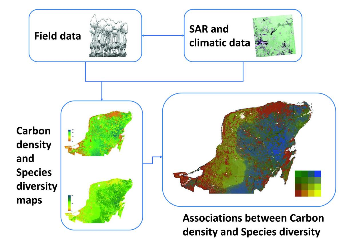
2.6. Generation of Carbon Density, Species Richness and Bivariate Maps

Maps of the spatial distribution of the response variables (carbon density and species richness), as well as their respective uncertainty maps, were generated. The species richness and carbon density maps were constructed using the random forest regression models obtained with the calibration dataset for all vegetation types (tropical dry forests and other vegetation types) and datasets of spatial predictors (HH, HV and NDBI, their texture metrics and the CWD). The maps were obtained with the “model.mapmake” function of the ModelMap library [50]. The uncertainty maps of species richness and AGB were built using the coefficient of variation (dividing the standard deviation by the mean). The random forest regression models computed the mean of all trees in the model for predicting each response variable, thereby allowing the calculation of standard deviations. Finally, the AGB map was converted to carbon density using a conversion factor of 0.516 [14].
A bivariate map that combined species richness and carbon density into a single map was created. The bivariate map of carbon density-species richness showed the number of species and the amount of carbon stock for each pixel in the study area. All three maps (carbon density, species richness and bivariate carbon density-species richness) used the Land Use Map from the Mexican National Institute of Statistics Geography and Information as a forest mask [51].
The mapped carbon density values for the entire Yucatan peninsula in this study were compared to previous studies that mapped carbon density or AGB in the same area [14,15]. The carbon density map of Cartus [14] was generated using canopy density estimates from Landsat, backscatter from ALOS-PALSAR and elevation derived from shuttle radar topography mission (STRM) as explanatory variables. Meanwhile, the AGB map obtained by Rodriguez–Veiga et al. [15] used vegetation indices derived from MODIS, backscatter from ALOS-PALSAR and elevation obtained from SRTM. Both studies used the NFI plots. However, they did not correct AGB values for small trees, or for temporal differences between field data collection and imagery acquisition. The comparison of the three AGB maps used the validation dataset described in Section 2.5 (854 plots) and the values of R2, RMSE, %RMSE and bias. In addition, we calculated the mean values and 95% confidence intervals of the differences between validation field plots and predicted AGB values of each map (Cartus et al. [14], Rodriguez–Veiga et al.) [15] and those obtained in this study) for different strata. The validation field data was stratified with AGB ranges every 50 Mg ha−1. We could not compare the tree species richness map since we could not find tree diversity maps of the Yucatan peninsula.

2.7. Statistical Analyses

A variance partitioning analysis was performed to analyze how each group of explanatory variables (backscatter, texture metrics from radar and climate) contributed to explaining the variability of the response variables (AGB and species richness). This analysis allowed us to identify the unique contribution of each group of variables, as well as their combined contribution. The first group of variables (backscatter) included HH, HV and the NDBI index. The second group (texture) comprised all texture metrics calculated for HH, HV and the DNBI index. The third group was the CWD index.
The total explained variance (using the three sets of explanatory variables) was divided into three non-overlapping fractions—the percentage of variance explained exclusively by the backscatter, texture or CDW groups, respectively, as well as the variance explained jointly by all three groups of explanatory variables—using the method proposed by Borcard et al. [52].
Finally, we computed Pearson correlation coefficients between carbon density and species richness maps, as well as field data (with 2847 sampling plots), at two extensions: one for the entire peninsula and the other for areas inside of different ecosystems. First, we calculated the correlations over the entire Yucatan Peninsula using all pixels of the carbon density and species richness maps and field data. Then, we calculated separate correlations for the three main types of tropical dry forest and for the other vegetation types, as shown in Figure 1C. Next, we calculated correlation within different areas, including mature vegetation, secondary vegetation with trees, shrubs or herbaceous-dominated cover for the TDF, mangrove forest, natural grasslands with some trees and wetlands areas for other vegetation types. Finally, we calculated the mean correlation and a 95% confidence interval for deciduous forests, semi-deciduous forests, semi-evergreen forests and other vegetation types.

3. Results

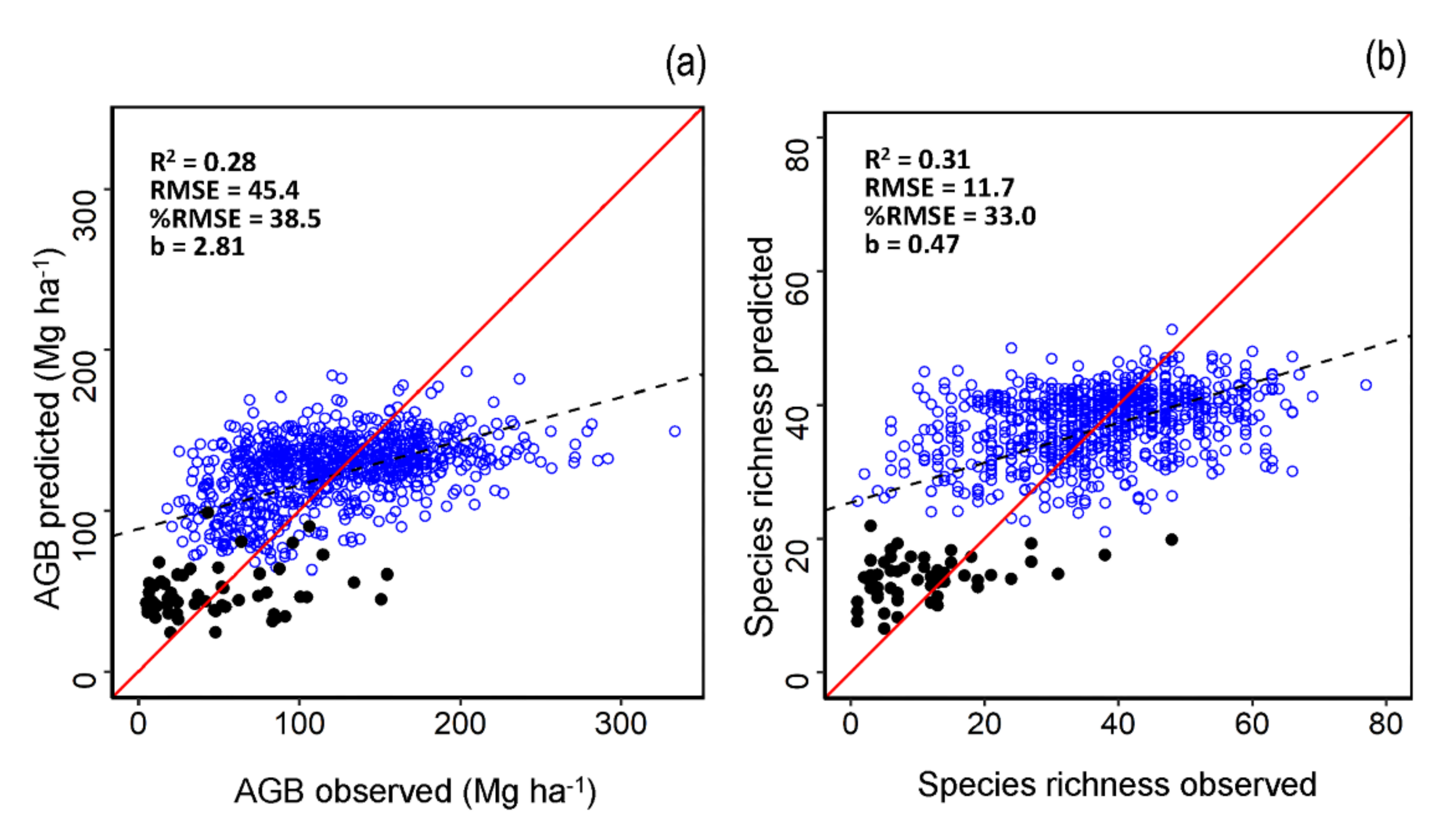
3.1. AGB and Species Richness Models Performance

The performances of the model predictions for AGB and species richness, using three sets of explanatory variables (backscatter, texture metrics from ALOS PALSAR and CWD) and using models that included all vegetation types (dry forest and other vegetation types), are shown in Table 2. The percentage of variance in AGB and species richness explained using the calibration data was moderate (R2 = 0.12 and 0.16). There was no significant spatial autocorrelation (p > 0.05) of residuals for any of the four models. The validation of the models indicated a better performance species richness than AGB. We obtained relative RMSE values of 38.5 and 33.0 for AGB and species richness, respectively (Table 2, Figure 2). Figure 2 shows that tropical dry forest and other vegetation types had two separated cluster of plots, where other vegetation types had higher errors for estimating AGB and species richness of trees.

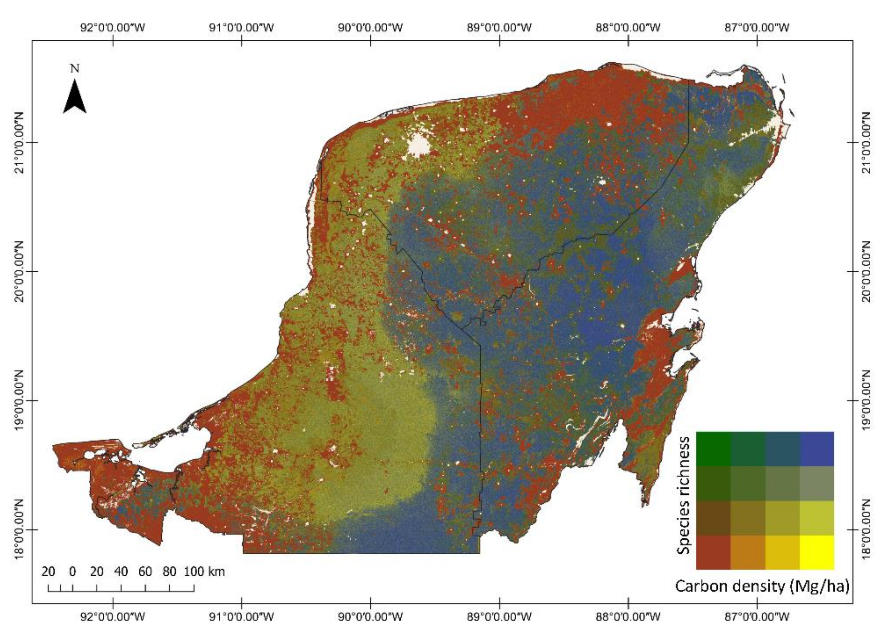
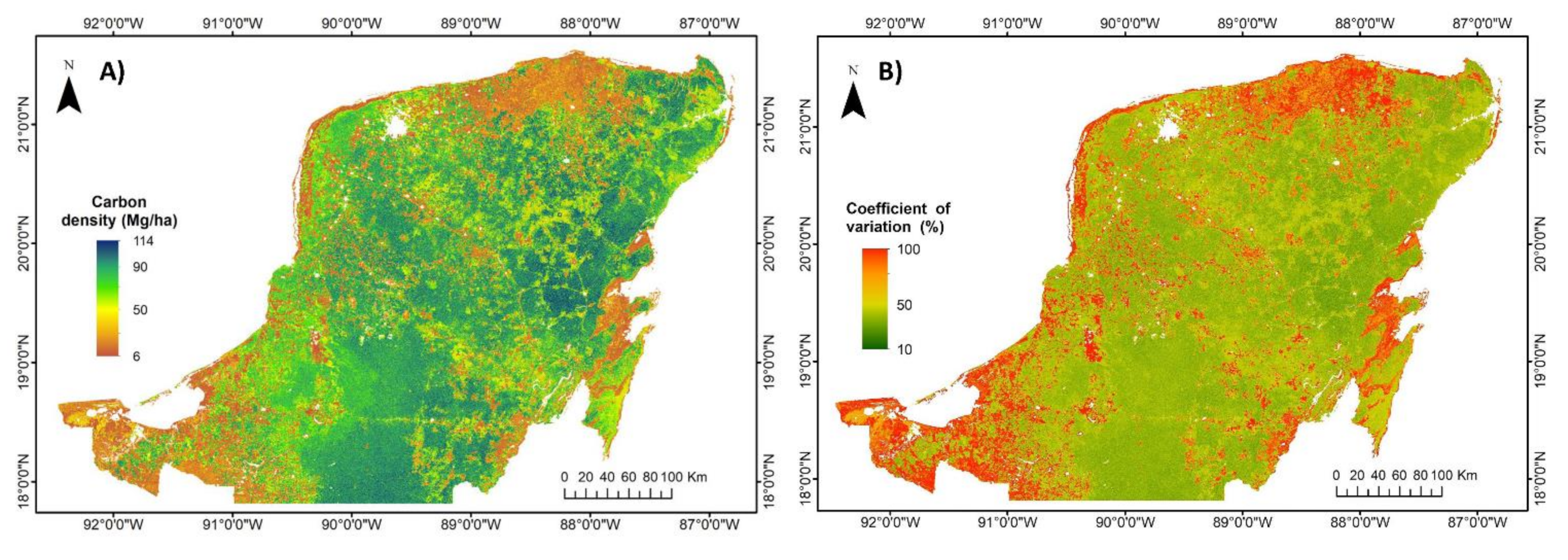
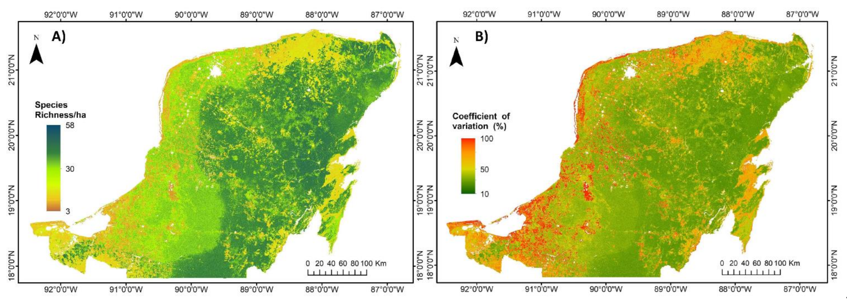
3.2. Regional Carbon Density, Species Richness and Bivariate Maps over the Yucatan Peninsula

The carbon density and species richness maps, as well as the bivariate carbon density-species richness map, were generated for the year 2015 with a pixel size of 25 m. These maps covered the entire Yucatan Peninsula. The carbon density map is shown in Figure 3A. The total carbon stored in the aboveground live biomass of the peninsula was estimated at 0.58 GT C. The highest carbon density values were located in the southwestern and southern portion, covered with semi-evergreen tropical dry forest, while the lowest carbon density values were located in the northeast and east of the peninsula, dominated by deciduous forest. However, there were still lower values of carbon density in other vegetation types. The highest uncertainty values corresponded to the other vegetation types (mangrove forest, natural grasslands with some trees, and wetlands). In contrast, in most of the tropical dry forests of the Yucatan Peninsula, the CV was below 40% (Figure 3B).
The species richness map showed similar patterns to the carbon density map (Figure 4A). In the tropical dry forest area, the semi-evergreen forest located in the southwest and south of the peninsula had the highest species richness compared to the deciduous and semi-deciduous forests. On the other hand, the class denoted as other vegetation types had the lowest number of tree species. The highest uncertainty values corresponded to the other vegetation types, whereas most of the area of TDF of the Yucatan Peninsula had CV values below 40% (Figure 4B).
The bivariate carbon density-species richness map exemplified the spatial relationships between carbon density and number of tree species, showing that 39.6% of the area in the peninsula had both high carbon stocks and high species richness. These areas (blue and gray colors in Figure 5) are located in the east of the peninsula. Conversely, 39.0% of the area in the peninsula showed low levels of carbon density and species richness (red, orange and brown in Figure 5). This means that there was a high congruence of carbon stocks and species richness in about 79.3% of area covered by the peninsula. The remaining 20.7% of peninsula is made up of areas with either high carbon density but low species richness (yellowish colors in Figure 5), or high species richness but low carbon density (green colors in Figure 5).

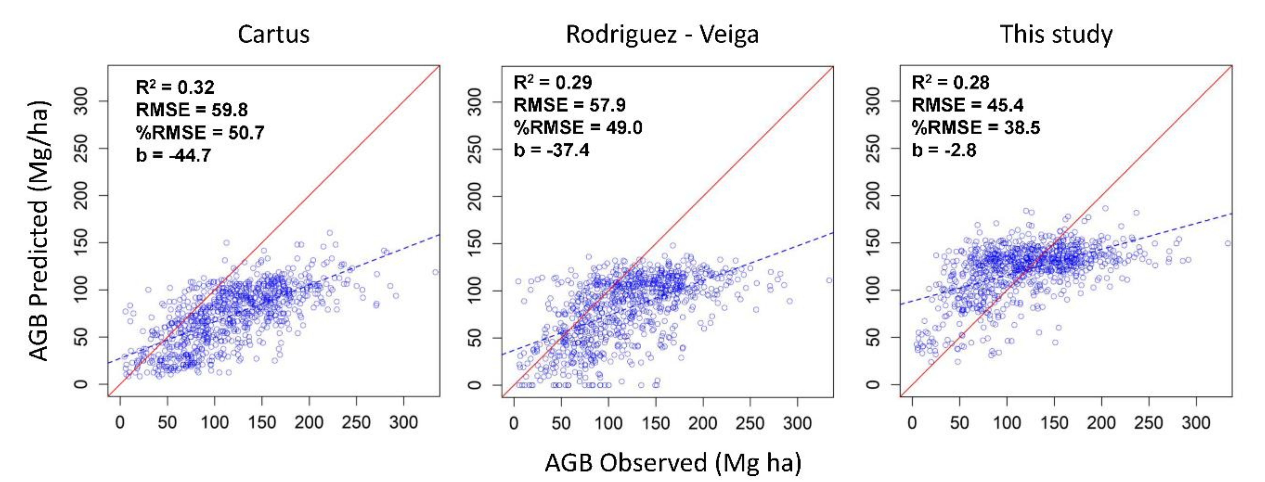
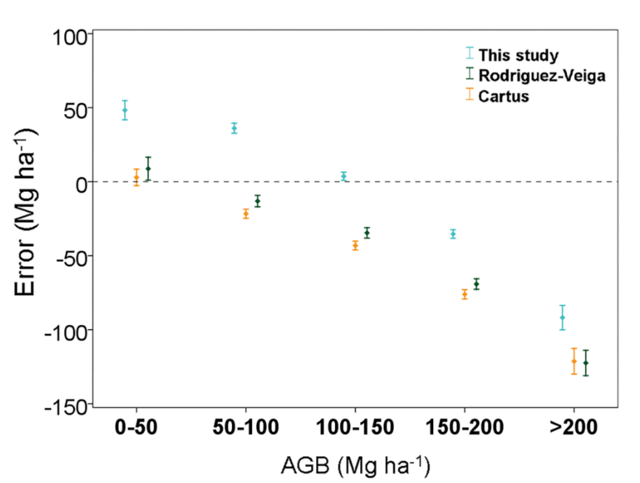
3.3. Comparison of the Aboveground Biomass Map with Previous Studies in the Yucatan Peninsula

The spatial distribution patterns of AGB in the Yucatan peninsula obtained in this study were similar to those obtained in previous studies [14,15]. However, when comparing the three maps with the independent validation dataset from NFI (which was previously corrected for small trees and time elapsed between field data collection and imagery acquisition), we noted some important differences. The agreement between observed and predicted values revealed a better performance for this study (%RMSE = 38.5 and bias = −2.8) compared with previous studies (%RMSE = 50.7 and bias = −44.7; %RMSE = 49.0 and bias = −37.4), respectively, for Cartus et al. [14] and Rodriguez-Veiga et al. [15] (Figure 6). Thus, the relative errors of this study were 12.7% and 10.5% lower than those of Cartus et al. [14] and Rodriguez-Veiga et al. [15], respectively. In addition, the bias in this study was low compared with the high negative bias values of the two previous studies, indicating a large underestimation of biomass in those studies.
Comparing the corrected validation plots with the AGB values in the three maps, we can see an overestimation of AGB in all maps at low biomass values (<50 Mg ha−1). However, our study also presented values of overestimation of AGB in biomass levels between 50 and 150 Mg ha−1. Our analysis also showed that all studies presented underestimations of AGB with biomass values larger than 150 g ha−1. Additionally, our study presented lower differences between field data and estimated AGB values than the previous ones. These differences are significant (Figure 7) and indicate that the other studies have higher underestimation of biomass.

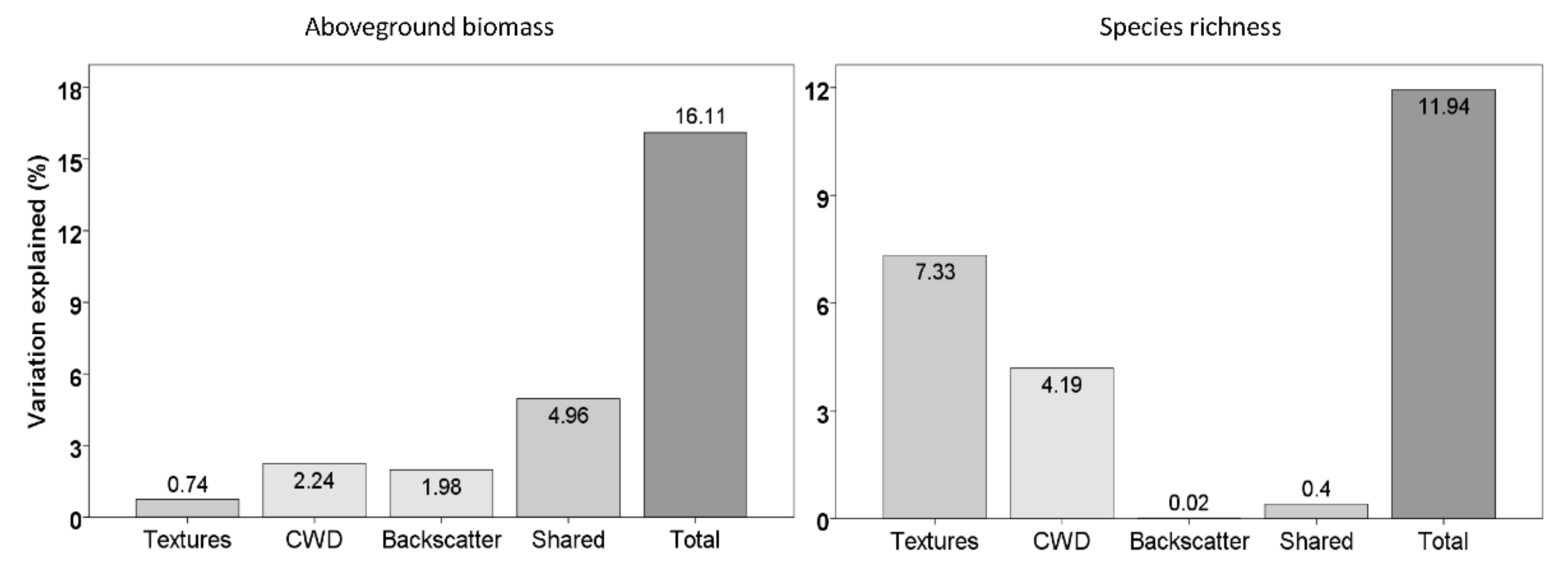
3.4. Importance of Variables to Estimate Carbon Density and Species Richness

Total variance, explained by the models that combined the three sets of explanatory variables, was higher for AGB than for species richness (16.1 and 11.9%, respectively). The variance partitioning analysis indicated that the three groups of variables jointly explained most of the variance of AGB (almost 5.0%). However, the backscatter and CWD variables exclusively explained more variation in AGB (2.0 and 2.3%) than texture metrics (0.7%). On the other hand, texture metrics and CWD (7.3 and 4.2%) exclusively explained a high percentage of variation in species richness compared to backscatter (0.02%) and to all three sets of variables (0.4) (Figure 8).

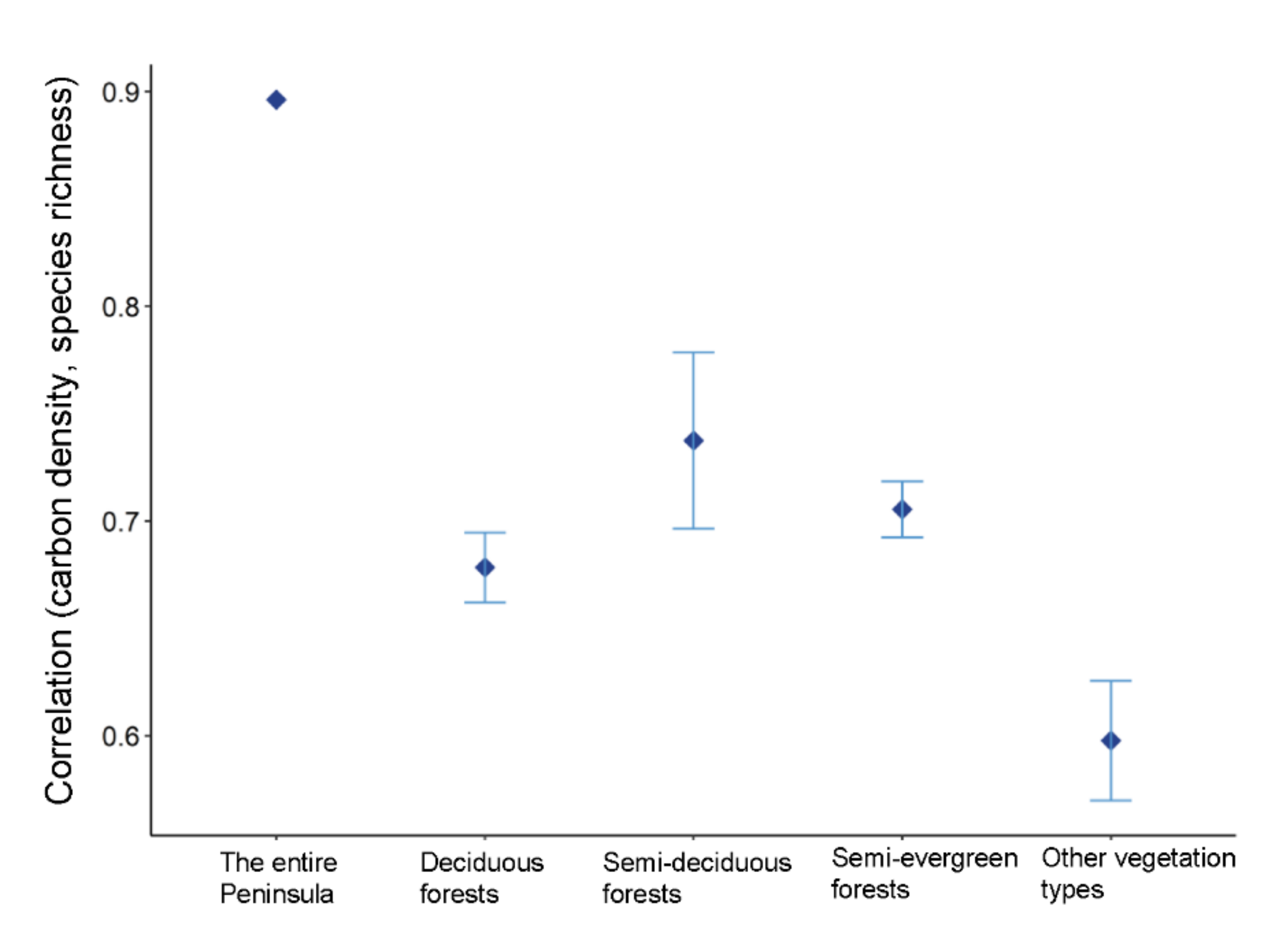
3.5. Relationships between Carbon Density and Species Richness

The correlation between carbon density and species richness of trees was high for the entire Yucatan Peninsula (r = 0.9 and r = 0.77 for the obtained map and field data, respectively). When analyzed by vegetation type, we found slightly lower correlations for the tropical dry, semi-deciduous (r = 0.74 and r = 0.68 for the obtained map and field data, respectively) and semi-evergreen forests (r = 0.71 and r = 0.64 for the obtained map and field data, respectively), with no significant differences between them. The deciduous forest had a significantly lower correlation (r = 0.68 and r = 0.57 for the obtained map and field data, respectively) than the semi-evergreen forest. The deciduous forest also had the lowest extension (1.16 million hectares) compared with the semi-deciduous and semi-evergreen forest (2.77 and 6.19 million hectares, respectively). Finally, the other vegetation types had the lowest correlation (r = 0.6 and r = 0.49 for the obtained map and field data, respectively) and the smallest area (13.30 million hectares) (Figure 9).

4. Discussion

4.1. Evaluation of Carbon Density and Species Richness Maps

To improve the accuracy of carbon density and tree species richness of regional maps, we corrected the field-estimated values of carbon density and species richness by accounting for small-sized trees and for the temporal differences between field data collection and imagery acquisition. We also explored the relationships between carbon density and tree species richness, estimated in the field with radar backscatter, radar texture metrics and climatic data. We found that validation models showed a moderately accurate relationship and low errors between observed and predicted values of carbon density and tree species richness (R2 = 0.28 and %RMSE = 38.5 and R2 = 0.31 and %RMSE = 33.0, respectively). We also found similar spatial patterns for carbon density and tree species richness estimations in tropical dry forests. These results concurred with those reported by Xu et al. [53] which generated a map of carbon density in the Democratic Republic of Congo, one of the largest countries with tropical forests. Authors reported a RMSE of 105 Mg ha−1 and an average of 280 Mg ha−1 of AGB at pixel level, having a R2 = 0.35 and %RMSE = 37.5. The relative error obtained for AGB in this study had similar or lower values compared with the accuracy assessment of regional AGB maps from other studies, which have reported relative RMSE from 37.0% to 67% at pixel level for Poland, Sweden and regions in Indonesia (Kalimantan), Mexico (Central Mexico and Yucatan peninsula), and South Africa (Eastern provinces) [24]. In a similar way, Su et al. [54] estimated AGB for China and reported a relative RMSE of 50.7% at pixel level. Meanwhile, Santoro et al. [55] estimated AGB globally at a 100 m resolution and reported a relative RMSE of 57.1% for tropical forest areas.
The representativeness of field data—that is, the amount and quality of information obtained from the NFI—was a key factor affecting the accuracy of our estimates of carbon density and species richness [24]. We therefore followed the methodology of Hernandez-Stefanoni et al. [23], who reported a reduction in relative errors of approximately 12% for AGB estimates when correcting NFI data for not including small-sized trees and for temporal differences between field and remotely sensed information. The regional uncertainty maps of carbon density and species richness showed the highest uncertainty values occurring in the other vegetation types (mangrove forests, natural grasslands with some trees and wetlands). In the same way, Figure 2 shows higher errors for estimating AGB and species richness for other vegetation types. The main reason for this high uncertainty is the low number of sample plots established for the other vegetation types class in the Mexican NFI [22], using a fixed grid of 10 × 10 km, compared to the grid of 5 × 5 km for tropical dry forest, and accounting for only 6.6% of the total number of plots in the Yucatan Peninsula (189 of 2847).
The accuracy of carbon density and species richness estimates could be significantly improved by increasing the number of sample field plots. Additional improvements in the accuracy of maps would be possible through the use of LiDAR plots with a two-stage upscaling method: first, relating field data with LiDAR metrics to map the variable of interest in areas covered by LiDAR, and then relating AGB (or species richness) estimated from LiDAR to satellite imagery and/or environmental information covering the entire area of interest. This approach has been applied successfully for estimating different vegetation attributes in several vegetation types [53,56]. Although there were some LiDAR data available for the Yucatan peninsula (collected by NASA’s G-LiHT airborne imager [57]) and the accuracy assessment of models relating AGB estimated in the field with LiDAR data revealed good performances (R2 = 0.85 and %RMSE = 19.7 and R2 = 0.85 and RMSE = 22.22 Mg ha−1, respectively, reported by Hernandez-Stefanoni et al. [23] and Urbazaev et al. [58]), the LiDAR data do not cover all the range of variability of biomass at field, so attempts to map AGB using the upscaling approach have been unsuccessful [23,58].
There are several maps of carbon density or AGB at the national scale in Mexico. The carbon density map of Cartus [14] reported, at a pixel level, an R2 from 0.2 to 0.5 depending on vegetation type and a relative RMSE of 54.0% and 63.0% on flat and steep slopes areas respectably. While, the AGB map obtained by Rodriguez-Veiga et al. [15] reported, at a pixel level, an R2 of 0.31 and a relative RMSE of 79.3%. These R2 values were comparable with the 0.28 obtained in this study, but their relative RMSE values were higher than the 38.5% reported in this study, indicating a better performance of the AGB map obtained herein. On the other hand, we also presented the first regional map of tree species richness over the Yucatan Peninsula.
Comparing the performance of the regional carbon density map obtained in this study and the cropped maps at Yucatan Peninsula from previous studies against corrected validation plots, we found similar model goodness of fit values but lower relative RMSE (R2 = 0.28 and %RMSE = 38.5, R2 = 0.29 and %RMSE = 49.0, R2 = 0.32 and %RMSE = 50.7 respectively for this study, Rodriguez-Veiga et al. [15] and Cartus el at. [14]). Thus, the relative errors in carbon density estimates of this study were 10.5% and 12.2% lower compared to the Rodriguez-Veiga and Cartus studies, respectively. Since the three maps were generated using the same field data, one of the main reasons for the differences in the accuracy of carbon density estimations among the three studies is that in this study, we corrected NFI-plot estimates. We also found that previous studies had higher negative values of bias compared to this study (bias = −2.8, −37.4 and −44.7 for this study, Rodriguez-Veiga et al. [15] and Cartus el at [14], respectively). Additionally, the map generated in this study underestimated AGB for biomass with values larger than 150 Mg ha−1, which is the general saturation level reported in several studies [59,60], while the other two maps underestimated AGB with values larger than 100 Mg ha−1. The underestimation of AGB in this study was significantly lower than in previous studies (Figure 7). This means that previous studies underestimated carbon density in the Yucatan Peninsula. These results suggested that the saturation in the SAR imagery could be reduced when using radar texture metrics and climatic data (water deficit) as explanatory variables. Texture metrics capture variations in vegetation structure in forest patches with different successional ages [27]. Water deficit is one of the most important factors regulating forest growth in tropical dry forests [32]. Other studies have also reported that using texture metrics from radar imagery, in addition to radar backscatter, can improve AGB estimates [61,62].
Finally, as we expected, carbon density was mostly associated with radar backscatter, while species richness was mostly related to radar texture metrics. The variance partitioning analysis indicated that the backscatter variables explained a larger percentage of variation in AGB (2.0%) compared to texture metrics (0.7%). Conversely, texture metrics had a higher influence on species richness (7.3%) compared to backscatter (0.02%). SAR sensors—such as ALOS PALSAR—with large wavelengths can easily penetrate the forest canopy, allowing accurate estimates of basal area, diameter and tree height, all which are related to biomass [63]. Meanwhile, texture metrics that measure spectral variability have been closely related to species richness [64], as these metrics are proxies of habitat heterogeneity. Greater heterogeneity of habitats allows the coexistence of a higher number of species [65].

4.2. Associations between Carbon Density and Species Richness in the Yucatan Peninsula

Forests managers, conservationists and decision makers are interested in mitigating climate change and conserving biodiversity simultaneously. In order to do that, it is of paramount importance that accurate regional information on the spatial distribution of carbon density and species richness is obtained [66]. That was the first goal of this study, achieved by reducing field estimate errors and combining radar backscatter, radar texture metrics and climatic data to obtain the corresponding maps. A second objective of this research was to generate spatial distributions of the relationship between carbon density and tree species richness for the tropical dry forests of the Yucatan Peninsula. Our results suggested that a large proportion of the peninsula contained high carbon density values, constituting important carbon stocks, as well as high tree species richness and, consequently, high relevance for biodiversity conservation. Indeed, we found that 39.6% of the forests in the peninsula possessed both high carbon density and high species richness of trees, which are mainly located in areas covered by semi-deciduous and semi-evergreen tropical dry forests (Figure 6). Other studies have also reported areas that are very rich, both in species diversity and in carbon stocks, in the Amazon [67].
Although carbon density and species richness of trees showed great variability across the Yucatan Peninsula, the overall correlation between both variables was high (r = 0.9, p < 0.0001), with 79.3% of the area showing a positive relationship, and only 20.7% a negative association. These results concurred with other studies that observed a positive association between these two variables in tropical forests distributed around the world [68] and in the Neotropics [32]. The results of this study also have practical implications for planning activities that simultaneously promote carbon maintenance and diversity conservation. However, this overall pattern hides some important differences among vegetation types. When we analyzed the association between carbon density and species richness by vegetation type, we found that those types with a lower spatial extent also showed lower correlations. Thus, the other vegetation types showed the lowest correlation (r = 0.6) and extent, followed by deciduous forest (r = 0.68), whereas the semi-deciduous and semi-evergreen forests, which had the largest spatial extent, had stronger correlations (r = 0.74 and r = 0.71, respectively). These patterns are likely observed because the association between carbon density (or species richness) and environmental variables is weaker when there is a comparatively small variability in environmental factors, such as that found in smaller spatial extents [69]. Finally, it is important to consider that the association between carbon density and species richness in this study was applied to trees. Other biological groups which are important components of biodiversity, including herbaceous plants, arthropods and soil (micro)organisms, should also be considered, as they may present different associations with forest carbon density.

5. Conclusions

In this study, we presented an improved carbon density map of forests across the Yucatan Peninsula with a pixel resolution of 25 m. We corrected field-estimated carbon density values from the Mexican national forest inventory, which allowed us to account for carbon stored in small-sized trees and for temporal differences between field data collection and imagery acquisition. This helped to reduce errors in estimating carbon density by 10.5% to 12.2%, compared to previous studies. In addition, the inclusion of texture metrics of L-band radar imagery, and the use of water deficits in the models, further contributed to reducing the estimation bias. This also reduced the saturation effects of radar imagery, since texture metrics can capture variations in the vegetation structures of forest fragments of different successional ages that differ in carbon density.
We also presented the first map of tree species richness over the Yucatan Peninsula with a spatial resolution of 25 m. This map followed the same approach as the carbon density map, relating tree species richness measured in the field with radar backscatter, texture metrics and climatic data using random forest regression models, as well as corrections of values from national forest inventory plots. The goodness of fit and relative RMSE of this map were similar to those of the carbon density map. As expected, the most important predictors of species richness were texture metrics of L-band radar backscatter, which measure spectral variability (used in this study as a proxy of habitat heterogeneity). By contrast, the backscatter of L-band radar, which relates closely with vegetation structure, was more important to explain variation in carbon density.
Finally, we mapped the spatial association between carbon density and species richness across the Yucatan Peninsula. We found a positive relationship in 79.3% of the study area, with 39.6% of the forests in the peninsula showing both high carbon densities and high species richness of trees. These forests are thus highly relevant for conserving biodiversity and, at the same time, averting climate change.

Author Contributions

Conceptualization, J.L.H.-S.; methodology, J.A.-M., J.L.H.-S.; writing—original draft preparation, J.L.H.-S.; writing—review and editing, M.Á.C.-S., C.A.P.-Q., F.T.-D. and J.M.D. All authors have read and agreed to the published version of the manuscript.

Funding

This research was funded by Ecometrica LTD and the United Kingdom Space Agency financed this research as part of the project Forests 2020.

Data Availability Statement

The ALOS PALSAR data used in this study was obtained from (https://www.eorc.jaxa.jp/ALOS/en/top/obs_top.htm, accessed on 10 August 2021). Data from the National Forest Inventory can be obtained by request to CONAFOR (Comisión Nacional Forestal, https://www.gob.mx/conafor, accessed on 1 August 2021).

Acknowledgments

We thank the Mexican National Forestry Commission (CONAFOR) for kindly providing forest inventory data.

Conflicts of Interest

The authors declare no conflict of interest.

References

  1. Poorter, L.; van der Sande, M.T.; Thompson, J.; Arets, E.J.; Alarcón, A.; Álvarez-Sánchez, J.; Ascarrunz, N.; Balvanera, P.; Barajas-Guzmán, G.; Boit, A.; et al. Diversity enhances carbon storage in tropical forests. Glob. Ecol. Biogeogr. 2015, 24, 1314–1328. [Google Scholar] [CrossRef]
  2. Keith, H.; Mackey, B.G.; Lindenmayer, D.B. Re-evaluation of forest biomass carbon stocks and lessons from the world’s most carbon-dense forests. Proc. Natl. Acad. Sci. USA 2009, 106, 11635–11640. [Google Scholar] [CrossRef] [PubMed] [Green Version]
  3. Portillo-Quintero, C.A.; Sánchez-Azofeifa, G.A. Extent and conservation of tropical dry forests in the Americas. Biol. Conserv. 2010, 143, 144–155. [Google Scholar] [CrossRef]
  4. Fine, P.V.A.; Ree, R.H.; Burnham, R.J. The disparity in tree species richness among tropical, temperate, and boreal biomes: The geographical area and age hypothesis. In Tropical Forest Community Ecology; Carson, R.P., Schnitzer, S.A., Eds.; Blackwell: Oxford, UK, 2008; pp. 31–45. [Google Scholar]
  5. Banda, K.; Delgado-Salinas, A.; Dexter, K.G.; Linares-Palomino, R.; Oliveira-Filho, A.; Prado, D.; Pullan, M.; Quintana, C.; Riina, R.; Rodríguez, G.M.; et al. Plant diversity patterns in neotropical dry forests and their conservation implications. Science 2016, 353, 1383–1387. [Google Scholar] [CrossRef] [Green Version]
  6. Friedlingstein, P.; Jones, M.W.; O’sullivan, M.; Andrew, R.M.; Hauck, J.; Peters, G.P.; Peters, W.; Pongratz, J.; Sitch, S.; Le Quéré, C.; et al. Global carbon budget 2019. Earth Syst. Sci. Data 2019, 11, 1783–1838. [Google Scholar] [CrossRef] [Green Version]
  7. Watson, J.E.; Dudley, N.; Segan, D.B.; Hockings, M. The performance and potential of protected areas. Nature 2014, 515, 67–73. [Google Scholar] [CrossRef]
  8. Saatchi, S.S.; Harris, N.L.; Brown, S.; Lefsky, M.; Mitchard, E.T.; Salas, W.; Zutta, B.R.; Buermann, W.; Lewis, S.L.; Hagen, S.; et al. Benchmark map of forest carbon stocks in tropical regions across three continents. Proc. Natl. Acad. Sci. USA 2011, 108, 9899–9904. [Google Scholar] [CrossRef] [Green Version]
  9. Baccini, A.G.S.J.; Goetz, S.J.; Walker, W.S.; Laporte, N.T.; Sun, M.; Sulla-Menashe, D.; Hackler, J.; Beck, P.S.A.; Dubayah, R.; Friedl, M.A.; et al. Estimated carbon dioxide emissions from tropical deforestation improved by carbon-density maps. Nat. Clim. Chang. 2012, 2, 182–185. [Google Scholar] [CrossRef]
  10. Kier, G.; Mutke, J.; Dinerstein, E.; Ricketts, T.H.; Küper, W.; Kreft, H.; Barthlott, W. Global patterns of plant diversity and floristic knowledge. J. Biogeogr. 2005, 32, 1107–1116. [Google Scholar] [CrossRef]
  11. Kreft, H.; Jetz, W. Global patterns and determinants of vascular plant diversity. Proc. Natl. Acad. Sci. USA 2007, 104, 5925–5930. [Google Scholar] [CrossRef] [PubMed] [Green Version]
  12. Houghton, R.A.; Hall, F.; Goetz, S.J. Importance of biomass in the global carbon cycle. J. Geophys. Res. Biogeosci. 2009, 114, 1–13. [Google Scholar] [CrossRef]
  13. Keil, P.; Chase, J.M. Global patterns and drivers of tree diversity integrated across a continuum of spatial grains. Nat. Ecol. Evol. 2019, 3, 390–399. [Google Scholar] [CrossRef]
  14. Cartus, O.; Kellndorfer, J.; Walker, W.; Franco, C.; Bishop, J.; Santos, L.; Fuentes, J. A national, detailed map of forest aboveground carbon stocks in Mexico. Remote. Sens. 2014, 6, 5559–5588. [Google Scholar] [CrossRef] [Green Version]
  15. Rodríguez-Veiga, P.; Saatchi, S.; Tansey, K.; Balzter, H. Magnitude, spatial distribution and uncertainty of forest biomass stocks in Mexico. Remote. Sens. Environ. 2016, 183, 265–281. [Google Scholar] [CrossRef] [Green Version]
  16. Réjou-Méchain, M.; Barbier, N.; Couteron, P.; Ploton, P.; Vincent, G.; Herold, M.; Mermoz, S.; Saatchi, S.; Chave, J.; de Boissieu, F.; et al. Upscaling Forest biomass from field to satellite measurements: Sources of errors and ways to reduce them. Surv. Geophys. 2019, 40, 881–911. [Google Scholar] [CrossRef]
  17. Marselis, S.M.; Abernethy, K.; Alonso, A.; Armston, J.; Baker, T.R.; Bastin, J.F.; Bogaert, J.; Boyd, D.S.; Boeckx, P.; Burslem, D.F.R.P.; et al. Evaluating the potential of full-waveform lidar for mapping pan-tropical tree species richness. Glob. Ecol. Biogeogr. 2020, 29, 1799–1816. [Google Scholar] [CrossRef]
  18. Dupuy, J.M.; Durán García, R.; García Contreras, G.; Arellano Morin, J.; Acosta Lugo, E.; Méndez González, M.E.; Andrade Hernandez, M. Chapter 8: Conservation and Use. In Biodiversity and Conservation of the Yuca-tán Peninsula; Islebe, G.A., Schmook, B., Calmé, S., León-Cortés, J.L., Eds.; Springer: Cham, Switzerland, 2015; pp. 1–5. [Google Scholar]
  19. Read, L.; Lawrence, D. Recovery of biomass following shifting cultivation in dry tropical forests of the Yucatan. Ecol. Appl. 2003, 13, 85–97. [Google Scholar] [CrossRef] [Green Version]
  20. Fricker, G.A.; Wolf, J.A.; Saatchi, S.S.; Gillespie, T.W. Predicting spatial variations of tree species richness in trop-ical forests from high-resolution remote sensing. Ecol. Appl. 2015, 25, 1776–1789. [Google Scholar] [CrossRef] [PubMed]
  21. Dupuy, J.M.; Hernández-Stefanoni, J.L.; Hernández-Juárez, R.A.; Tetetla-Rangel, E.; López-Martínez, J.O.; Leyequién-Abarca, E.; May-Pat, F. Patterns and correlates of tropical dry forest structure and composition in a highly replicated chronosequence in Yucatan, Mexico. Biotropica 2012, 44, 151–162. [Google Scholar] [CrossRef]
  22. CONAFOR. Inventario nacional forestal y de suelos. Inf. Result. 2018, 1, 2009–2014. [Google Scholar]
  23. Hernández-Stefanoni, J.L.; Castillo-Santiago, M.Á.; Mas, J.F.; Wheeler, C.E.; Andres-Mauricio, J.; Tun-Dzul, F.; George-Chacón, S.P.; Reyes-Palomeque, G.; Castellanos-Basto, B.; Vaca, R.; et al. Improving aboveground biomass maps of tropical dry forests by integrating LiDAR, ALOS PALSAR, climate and field data. Carbon Balance Manag. 2020, 15, 1–17. [Google Scholar] [CrossRef] [PubMed]
  24. Rodríguez-Veiga, P.; Quegan, S.; Carreiras, J.; Persson, H.J.; Fransson, J.E.; Hoscilo, A.; Ziółkowski, D.; Stereńczak, K.; Lohberger, S.; Stängel, M.; et al. Forest biomass retrieval approaches from earth observation in different biomes. Int. J. Appl. Earth Obs. Geoinf. 2019, 77, 53–68. [Google Scholar] [CrossRef]
  25. Wang, R.; Gamon, J.A. Remote sensing of terrestrial plant biodiversity. Remote. Sens. Environ. 2019, 231, 111218. [Google Scholar] [CrossRef]
  26. Ploton, P.; Barbier, N.; Couteron, P.; Antin, C.M.; Ayyappan, N.; Balachandran, N.; Barathan, N.; Bastin, J.F.; Chuyong, G.; Dauby, G.; et al. Toward a general trop-ical forest biomass prediction model from very high resolution optical satellite images. Remote. Sens. Environ. 2017, 200, 140–153. [Google Scholar] [CrossRef]
  27. Thapa, R.B.; Watanabe, M.; Motohka, T.; Shimada, M. Potential of high-resolution ALOS–PALSAR mosaic texture for aboveground forest carbon tracking in tropical region. Remote. Sens. Environ. 2015, 160, 122–133. [Google Scholar] [CrossRef]
  28. Joshi, N.; Mitchard, E.T.; Brolly, M.; Schumacher, J.; Fernández-Landa, A.; Johannsen, V.K.; Marchamalo, M.; Fensholt, R. Understanding ‘saturation’of radar signals over forests. Sci. Rep. 2017, 7, 1–11. [Google Scholar] [CrossRef] [Green Version]
  29. Rocchini, D.; Balkenhol, N.; Carter, G.A.; Foody, G.M.; Gillespie, T.W.; He, K.S.; Kark, S.; Levin, N.; Lucas, K.; Luoto, M.; et al. Remotely sensed spectral heterogeneity as a proxy of species diversity: Recent advances and open challenges. Ecol. Inform. 2010, 5, 318–329. [Google Scholar] [CrossRef]
  30. Stein, A.; Gerstner, K.; Kreft, H. Environmental heterogeneity as a universal driver of species richness across taxa, biomes and spatial scales. Ecol. Lett. 2014, 17, 866–880. [Google Scholar] [CrossRef] [PubMed]
  31. George-Chacon, S.P.; Dupuy, J.M.; Peduzzi, A.; Hernandez-Stefanoni, J.L. Combining high resolution satellite imagery and lidar data to model woody species diversity of tropical dry forests. Ecol. Indic. 2019, 101, 975–984. [Google Scholar] [CrossRef]
  32. Poorter, L.; Bongers, F.; Aide, T.M.; Zambrano, A.M.A.; Balvanera, P.; Becknell, J.M.; Boukili, V.; Brancalion, P.H.S.; Broadbent, E.N.; Chazdon, R.L.; et al. Biomass resili-ence of Neotropical secondary forests. Nature (London) 2016, 530, 211–214. [Google Scholar] [CrossRef]
  33. Rozendaal, D.M.A.; Bongers, F.; Aide, T.M.; Alvarez-Dávila, E.; Ascarrunz, N.; Balvanera, P.; Becknell, J.M.; Bentos, T.V.; Brancalion, P.H.S.; Cabral, G.A.L.; et al. Biodiversity recovery of Neotropical secondary forests. Sci. Adv. 2019, 5, eaau3114. [Google Scholar] [CrossRef] [PubMed] [Green Version]
  34. Mittelbach, G.G.; Steiner, C.F.; Scheiner, S.M.; Gross, K.L.; Reynolds, H.L.; Waide, R.B.; Willig, W.R.; Dodson, S.I.; Gough, L. What is the observed relationship between species richness and productivity? Ecology 2001, 82, 2381–2396. [Google Scholar] [CrossRef]
  35. Sullivan, M.J.; Talbot, J.; Lewis, S.L.; Phillips, O.L.; Qie, L.; Begne, S.K.; Chave, J.; Cuni-Sanchez, A.; Hubau, W.; Lopez-Gonzalez, G.; et al. Diversity and carbon storage across the tropical forest biome. Sci. Rep. 2017, 7, 1–12. [Google Scholar] [CrossRef] [Green Version]
  36. Murray, J.P.; Grenyer, R.; Wunder, S.; Raes, N.; Jones, J.P. Spatial patterns of carbon, biodiversity, deforestation threat, and REDD+ projects in Indonesia. Conserv. Biol. 2005, 29, 1434–1445. [Google Scholar] [CrossRef] [Green Version]
  37. Ramírez Ramírez, G.; Dupuy Rada, J.M.; Ramírez y Avilés, L.; Solorio Sánchez, F.J. Evaluación de ecuaciones alométricas de biomasa epigea en una selva mediana subcaducifolia de Yucatán. Madera bosques 2017, 23, 163–179. [Google Scholar] [CrossRef] [Green Version]
  38. Chave, J.; Andalo, C.; Brown, S.; Cairns, M.A.; Chambers, J.Q.; Eamus, D.; Fölster, H.; Fromard, F.; Higuchi, N.; Kira, T.; et al. Tree allometry and improved estimation of carbon stocks and balance in tropical forests. Oecologia 2005, 145, 87–99. [Google Scholar] [CrossRef]
  39. Guyot, J. Estimation du Stock de Carbone dans la Végétation des Zones Humides de la Péninsule du Yucatan. Memoire de fin d’etudes. Licentiate Thesis, AgroParis Tech-El Colegio de la Frontera Sur, Chiapas, Mexico, 2011; p. 110. [Google Scholar]
  40. Cairns, M.A.; Olmsted, I.; Granados, J.; Argaez, J. Composition and aboveground tree biomass of a dry semi-evergreen forest on Mexico’s Yucatan Peninsula. For. Ecol. Manag. 2003, 186, 125–132. [Google Scholar] [CrossRef]
  41. Urquiza-Haas, T.; Dolman, P.M.; Peres, C.A. Regional scale variation in forest structure and biomass in the Yucatan Peninsula, Mexico: Effects of forest disturbance. For. Ecol. Manag. 2007, 247, 80–90. [Google Scholar] [CrossRef]
  42. Chave, J.; Condit, R.; Lao, S.; Caspersen, J.P.; Foster, R.B.; Hubbell, S.P. Spatial and temporal variation of biomass in a tropical forest: Results from a large census plot in Panama. J. Ecol. 2003, 91, 240–252. [Google Scholar] [CrossRef]
  43. Frangi, J.L.; Lugo, A.E. Ecosystem dynamics of a subtropical floodplain forest. Ecol. Monogr. 1985, 55, 351–369. [Google Scholar] [CrossRef]
  44. Shimada, M.; Ohtaki, T. Generating Large-Scale High-Quality SAR Mosaic Datasets: Application to PALSAR Data for Global Monitoring. IEEE J. Sel. Top. Appl. Earth Obs. Remote. Sens. 2010, 3, 637–656. [Google Scholar] [CrossRef]
  45. Almeida-Filho, R.; Shimabukuro, Y.E.; Rosenqvist, A.; Sánchez, G.A. Using dual-polarized ALOS PALSAR data for detecting new fronts of deforestation in the Brazilian Amazônia. Int. J. Remote. Sens. 2009, 30, 3735–3743. [Google Scholar] [CrossRef]
  46. Mitchard, E.T.A.; Saatchi, S.S.; White, L.J.T.; Abernethy, K.A.; Jeffery, K.J.; Lewis, S.L.; Collins, M.; Lefsky, M.A.; Leal, M.E.; Woodhouse, I.H.; et al. Mapping tropical forest biomass with radar and spaceborne LiDAR in Lopé National Park, Gabon: Overcoming problems of high biomass and persistent cloud. Biogeosciences 2012, 9, 179–191. [Google Scholar] [CrossRef] [Green Version]
  47. Haralick, R.M.; Dinstein, I.; Shanmugam, K. Textural Features for Image Classification. IEEE Trans. Syst. Man Cybern. 1973, SMC-3, 610–621. [Google Scholar] [CrossRef] [Green Version]
  48. Fischer, R.; Knapp, N.; Bohn, F.; Shugart, H.H.; Huth, A. The relevance of forest structure for biomass and productivity in temperate forests: New perspectives for remote sensing. Surv. Geophys. 2019, 40, 709–734. [Google Scholar] [CrossRef]
  49. Zvoleff, A. Calculate Textures from Grey-Level Co-Occurrence Matrices (GLCMs); R Package v 1.6.4; R. Package: Arlington, VA, USA, 2019. [Google Scholar]
  50. Freeman, E.A.; Frescino, T.S.; Moisen, G.G. ModelMap: And R Package for Model Creation and Map Production. 2018, p. 18. Available online: https://cran.r-project.org/web/packages/ModelMap/vignettes/VModelMap (accessed on 10 August 2021).
  51. INEGI. Conjunto Nacional de Uso del Suelo y Vegetación a escala 1:250,000, Serie IV; INEGI: Aguascalientes, Mexico, 2010. [Google Scholar]
  52. Borcard, D.; Legendre, P.; Avois-Jacquet, C.; Tuomisto, H. Disecting the spatial structure of ecological data al multiple scales. Ecology 2004, 85, 1826–1832. [Google Scholar] [CrossRef] [Green Version]
  53. Xu, L.; Saatchi, S.S.; Shapiro, A.; Meyer, V.; Ferraz, A.; Yang, Y.; Bastin, J.F.; Banks, N.; Boeckx, P.; Verbeeck, H.; et al. Spatial distribution of carbon stored in forests of the Democratic Republic of Congo. Sci. Rep. 2017, 7, 1–12. [Google Scholar] [CrossRef] [Green Version]
  54. Su, Y.; Guo, Q.; Xue, B.; Hu, T.; Alvarez, O.; Tao, S.; Fang, J. Spatial distribution of forest aboveground biomass in China: Estimation through combination of spaceborne lidar, optical imagery, and forest inventory data. Remote. Sens. Environ. 2016, 173, 187–199. [Google Scholar] [CrossRef] [Green Version]
  55. Santoro, M.; Cartus, O.; Carvalhais, N.; Rozendaal, D.; Avitabilie, V.; Araza, A.; De Bruin, S.; Herold, M.; Quegan, S.; Veiga, P.R.; et al. The global forest above-ground biomass pool for 2010 estimated from high-resolution satellite observations. Earth Syst. Sci. Data Discuss. 2020, 148, 1–38. [Google Scholar] [CrossRef]
  56. Luther, J.E.; Fournier, R.A.; van Lier, O.R.; Bujold, M. Extending ALS-based mapping of forest attributes with medium resolution satellite and environmental data. Remote. Sens. 2019, 11, 1092. [Google Scholar] [CrossRef] [Green Version]
  57. Cook, B.; Nelson, R.; Middleton, E.; Morton, D.; McCorkel, J.; Masek, J.; Ranson, K.; Ly, V.; Montesano, P. NASA Goddard’s LiDAR, hyperspectral and thermal (G-LiHT) airborne imager. Remote. Sens. 2013, 5, 4045–4066. [Google Scholar] [CrossRef] [Green Version]
  58. Urbazaev, M.; Thiel, C.; Cremer, F.; Dubayah, R.; Migliavacca, M.; Reichstein, M.; Schmullius, C. Estimation of forest aboveground biomass and uncertainties by integration of field measurements, airborne LiDAR, and SAR and optical satellite data in Mexico. Carbon Balance Manag. 2018, 13, 1–20. [Google Scholar] [CrossRef] [PubMed] [Green Version]
  59. Mermoz, S.; Réjou-Méchain, M.; Villard, L.; Le Toan, T.; Rossi, V.; Gourlet-Fleury, S. Decrease of L-band SAR backscatter with biomass of dense forests. Remote. Sens. Environ. 2015, 159, 307–317. [Google Scholar] [CrossRef]
  60. Morel, A.C.; Saatchi, S.S.; Malhi, Y.; Berry, N.J.; Banin, L.; Burslem, D.; Nilus, R.; Ong, R.C. Estimating aboveground biomass in forest and oil palm plantation in Sabah, Malaysian Borneo using ALOS PALSAR data. For. Ecol. Manag. 2011, 262, 1786–1798. [Google Scholar] [CrossRef]
  61. Champion, I.; Germain, C.; Da Costa, J.P.; Alborini, A.; Dubois-Fernandez, P. Retrieval of forest stand age from SAR image texture for varying distance and orientation values of the gray level co-occurrence matrix. IEEE Geosci. Remote. Sens-Ing Lett. 2014, 11, 5–9. [Google Scholar] [CrossRef] [Green Version]
  62. Sarker, M.L.R.; Nichol, J.; Iz, H.B.; Ahmad, B.B.; Rahman, A.A. Forest biomass estimation using texture measurements of high-resolution dual-polarization C-band SAR data. IEEE Trans. Geosci. Remote. Sens. 2013, 51, 3371–3384. [Google Scholar] [CrossRef]
  63. Andres-Mauricio, J.; Valdez-Lazalde, J.R.; George-Chacón, S.P.; Hernández-Stefanoni, J.L. Mapping structural attributes of tropical dry forests by combining Synthetic Aperture Radar and high-resolution satellite imagery data. Appl. Veg. Sci. 2021, 24, e12580. [Google Scholar] [CrossRef]
  64. Rocchini, D.; Boyd, D.S.; Féret, J.B.; Foody, G.M.; He, K.S.; Lausch, A.; Nagendra, H.; Wegmann, M.; Pettorelli, N. Satellite remote sensing to monitor species diversity: Potential and pitfalls. Remote. Sens. Ecol. Conserv. 2016, 2, 25–36. [Google Scholar] [CrossRef]
  65. Palmer, M.W.; Earls, P.G.; Hoagland, B.W.; White, P.S.; Wohlgemuth, T. Quantitative tools for perfecting species lists. Environmetrics 2002, 13, 121–137. [Google Scholar] [CrossRef]
  66. Soto-Navarro, C.; Ravilious, C.; Arnell, A.; De Lamo, X.; Harfoot, M.; Hill, S.L.L.; Wearn, O.R.; Santoro, M.; Bouvet, A.; Mermoz, S.; et al. Mapping co-benefits for carbon storage and biodiversity to inform conservation policy and action. Philos. Trans. R. Soc. B 2020, 375, 20190128. [Google Scholar] [CrossRef] [Green Version]
  67. Strassburg, B.B.; Kelly, A.; Balmford, A.; Davies, R.G.; Gibbs, H.K.; Lovett, A.; Miles, L.; Orme, C.D.L.; Price, J.; Turner, R.K.; et al. Global congruence of carbon storage and biodiversity in terrestrial ecosystems. Conserv. Lett. 2010, 3, 98–105. [Google Scholar] [CrossRef] [Green Version]
  68. Cavanaugh, K.C.; Gosnell, J.S.; Davis, S.L.; Ahumada, J.; Boundja, P.; Clark, D.B.; Mugerwa, B.; Jansen, P.A.; O’Brien, T.G.; Rovero, F.; et al. Carbon storage in tropical forests correlates with taxonomic diversity and functional dominance on a global scale. Glob. Ecol. Biogeog-Raphy 2014, 23, 563–573. [Google Scholar] [CrossRef]
  69. Di Marco, M.; Watson, J.E.; Currie, D.J.; Possingham, H.P.; Venter, O. The extent and predictability of the biodiversity–carbon correlation. Ecol. Lett. 2018, 21, 365–375. [Google Scholar] [CrossRef] [Green Version]
Figure 1. Location of the study area and field plots distribution: (A) the spatial distribution National Forest Inventory (NFI) field plots in the study area, (B) location of the Yucatan Peninsula, (C) distribution of the main vegetation types in the peninsula.
Remotesensing 13 03179 g001
Figure 2. Comparison of observed versus predicted values for aboveground biomass (AGB) (a) and species richness of trees (b). Red lines are reference lines 1:1, while dashed lines are regression lines. The coefficient of determination (R2), the Root-Mean-Square Error (RMSE), the Percentage of Root-Mean-Square Error (%RMSE) and the bias were calculated using both vegetation classes (tropical dry forests and other vegetation types). Open blue circles represent forest plots, while filled black circles correspond to other vegetation-type plots.
Remotesensing 13 03179 g002
Figure 3. Estimated map of the aboveground carbon density for the entire Yucatan Peninsula (A) and the uncertainty map, measured with coefficient of variation (B).
Remotesensing 13 03179 g003
Figure 4. Estimated map of the species richness for the entire Yucatan Peninsula (A) and the uncertainty map measured with coefficient of variation (B).
Remotesensing 13 03179 g004
Figure 5. Map of the Yucatan Peninsula showing congruence between carbon density and species richness of trees. The hotspot areas that have high values for both carbon density and species richness are shown in blue.
Remotesensing 13 03179 g005
Figure 6. Observed versus predicted values for aboveground biomass in the maps generated in this study compared to the maps of Cartus el at. [14] and Rodriguez-Veiga et al. [15] for the Yucatan Peninsula. Red lines are reference lines 1:1, while dashed lines are regression lines.
Remotesensing 13 03179 g006
Figure 7. Mean values and 95% confidence intervals obtained as the differences between NFI field data plots used for validation and predicted AGB values of this study, and those of Cartus et al. [14] and Rodriguez-Veiga et al. [15] for different categorical AGB values.
Remotesensing 13 03179 g007
Figure 8. Variance partitioning analysis of the calibrated models to predict aboveground biomass and species richness from three groups of explanatory variables: (1) backscatter (HH, HV and NDBI index), (2) texture metrics from radar and (3) CWD (climatic water deficit).
Remotesensing 13 03179 g008
Figure 9. Correlation between carbon density and species richness for the entire peninsula and for different vegetation types: deciduous, semi-deciduous and semi-evergreen tropical dry forest forests and other vegetation types (mangrove forest, natural grasslands with some trees and wetlands). The diamonds represent the mean values and the lines 95% confidence intervals.
Remotesensing 13 03179 g009
Table 1. Allometric equations used to estimate aboveground biomass for the most important vegetation types and plant growth forms in the Yucatán Peninsula.
Author of EquationType of VegetationGrowth Form/Class Size
Ramírez et al. [37]Deciduos and semi-deciduous forest Tree/DBH < 10 cm
Chave et al. [38]Deciduos and semi-deciduous forest Tree/DBH ≥ 10 cm
Guyot [39]Semi-evergreen forestTree/DBH < 10 cm
Cairns modified [40] by Urquiza-Haas et al. [41]Semi-evergreen forestTree/DBH ≥ 10 cm
Chave et al. [42]Mangrove forestTree
Chave et al. [42]Deciduos and semi-deciduos forestLiana
Frangi and Lugo [43]Deciduos, semi-deciduos and semi-evergreen forestPalm/DBH ≥ 10 cm
Table 2. Random forest statistics for calibration and validation models of aboveground biomass (AGB) and species richness.
VariableType of DataNumber of PlotsR2RMSE%RMSE
AGBCalibration19930.1647.638.1
Validation8540.2845.438.5
Species RichnessCalibration19930.1212.031.9
Validation8540.3111.7233.0
Publisher’s Note: MDPI stays neutral with regard to jurisdictional claims in published maps and institutional affiliations.

