Abstract
The detection of elongated objects, such as ships, from satellite images has very important application prospects in marine transportation, shipping management, and many other scenarios. At present, the research of general object detection using neural networks has made significant progress. However, in the context of ship detection from remote sensing images, due to the elongated shape of ship structure and the wide variety of ship size, the detection accuracy is often unsatisfactory. In particular, the detection accuracy of small-scale ships is much lower than that of the large-scale ones. To this end, in this paper, we propose a hierarchical scale sensitive CenterNet (HSSCenterNet) for ship detection from remote sensing images. HSSCenterNet adopts a multi-task learning strategy. First, it presents a dual-direction vector to represent the posture or direction of the tilted bounding box, and employs a two-layer network to predict the dual direction vector, which improves the detection block of CenterNet, and cultivates the ability of detecting targets with tilted posture. Second, it divides the full-scale detection task into three parallel sub-tasks for large-scale, medium-scale, and small-scale ship detection, respectively, and obtains the final results with non-maximum suppression. Experimental results show that, HSSCenterNet achieves a significant improved performance in detecting small-scale ship targets while maintaining a high performance at medium and large scales.
1. Introduction
With the rapid development of artificial intelligence, object detection has witnessed great progress in many application scenarios [1]. One of the applications is the ship detection from remote sensing images [2,3,4,5,6,7]. In the past two decades, a number of commercial and government optical satellites have been deployed to observe the earth, which provide massive amounts of optical remote sensing images [8,9,10]. With the increasing importance of sea transportation, ship detection from remote sensing images can bring commercial values in many fields, e.g., marine transportation, marine fishing, maritime search and rescue, sea area security, and military reconnaissance, etc. Meanwhile, ship detection can also be applied to inland rivers and lakes, and benefit to economic planning, e.g., environmental monitoring, construction planning, and shipping management.
Owing to the powerful representation ability of deep convolutional neural networks (DCNNs), object detection from natural images has achieved great success [11,12,13,14,15]. Compared with traditional detectors, DCNN-based detectors have increased the accuracy by 62%, reaching 83.8%, on the VOC dataset [16,17]. So far, a CNN-based object detector can be divided into two parts: the backbone network and the box head [18,19]. The backbone network extracts convolution features from the input image, and then the box head receives the convolution features and generates the detection results [20]. According to whether the box head uses predefined bounding boxes, the detectors can be divided into two categories: anchor-based and anchor-free. The anchor-based methods generate a large number of pre-set fixed bounding boxes (proposals) on the convolution features. A bounding box is composed of the closest anchor box and the offset of the actual box from the anchor. The network does not directly predict the coordinates of the object box. It predicts the offset between the object box and the anchor box, and combines the anchor box coordinates and the offset to obtain the final result. The anchor-free methods give up the dense paving of pre-set boxes, but uses one or multiple key points to indicate the position of the target box on the image. It converts the predictions of box coordinates into predictions of key points.
According to whether the location prediction and the object-label prediction are performed at the same time, the anchor-based methods can be further divided into two categories: one-stage methods and two-stage methods. The two-stage methods first use a region proposal network (RPN) to predict possible target candidate proposals, and then determine the object label in these candidate proposals. The single-stage methods predict the location of the target object and determine the label at the same time without RPN. The anchor-free methods generally perform box prediction and label classification at the same time.
However, the detection performance of small targets is still a bottleneck that is difficult to break through, and the detection accuracy is far below the average. When using optical remote sensing images to detect ships on the water, the detection problem of small targets is even more prominent. First, when the ship target is very small, it appears as a small group of pixels on the image, the outer contour becomes very blurred, and it is difficult to distinguish the shape features. This makes small target ships very easy to confuse in the background. Second, remote sensing images are taken by satellite or airborne optical imaging equipment facing the surface of the earth, with a very broad field of view. Oceans, cities, land, grasslands, and deserts can all become the image background. Therefore, there are a lot of areas in the image background that have similar characteristics to small target ships, which can easily become the false positives in the detection. These factors heavily increase the difficulties of ship detection from remote sensing images.
In recent years, some strategies were proposed to improve the performance of small object detection, e.g., feature pyramid fusion [21,22], normalized multi-scale training [23,24], context modeling [25,26], and adversarial learning [27,28,29], etc. However, most methods are based on horizontal bounding boxes. In our opinion, for small ship detection, the use of tilted bounding boxes holds more advantages than horizontal bounding boxes. First, the ship target has a long and thin shape, and the boundary of the tilted bounding boxes can be close to the ship boundary, avoiding the introduction of redundant background information. Second, ship targets are often arranged close to each other, and the tilted bounding boxes can also be similarly arranged, avoiding the problem of overlapping in case of horizontal boxes. Third, the tilted bounding boxes can additionally provide the orientation information as comparing to the traditional horizontal bounding boxes.
Based on the discussion above, we first propose a dual direction vector, which provides a new way to express the attitude or direction of the tilted bounding box. Based on this vector, we improve the detection block by adding a two-layer network to predict the dual direction vector, which allows detecting objects with tilted bounding boxes. Then, we build a hierarchical scale-sensitive network on the CenterNet [30] for object detection. We name the proposed network as HSSCenterNet. Using a multi-task learning strategy, it divides the full-scale detection task into three sub-tasks: small-scale, medium-scale, and large-scale object detection, where three parallel branches are designed for the three tasks. When training the HSSCenterNet model, a target sample selection mechanism is presented for the detection network: the weight parameters of the detection branches of each scale are calculated and updated by the target samples of their respective scales; the weight parameters of the basic network part are calculated by the full-scale. Finally, results of the three detection branches are merged together, and the final results are obtained by a non-maximum suppression algorithm.
2. Related Work
In this section, we briefly overview the related work on convolutional neural network-based small-object detection technologies.
2.1. Small Object Detection Technology Based on Feature Pyramid Fusion
A number of studies on convolutional networks show that the shallow convolutional feature map is more suitable for detecting small targets. If it detects large targets, it only ‘sees’ a part of the targets. The deep feature map has a large receptive field and is suitable for detecting large targets. If it detects small targets, it ‘sees’ too much background information and too many redundant noise signals.
To this end, Lin et al. proposed a feature pyramid networks (FPN) for object detection [21]. If the convolution feature maps generated by the main part of the detection model is arranged from a top-bottom order, i.e., from deep to shallow, a pyramid structure can be formed. From top to bottom of the feature pyramid, each layer of features is convolved to make the number of channels the same after convolution, and then the feature map of the previous layer enlarged twice in size is added, and finally through convolution to attain the fusion feature. Through this connection, the convolution feature map can fuse features of different resolutions and different semantic strengths. At the same time, as this method only adds extra cross-layer connections in the original network backbone, it hardly adds extra computation cost in practical applications. However, the feature pyramid will undermine the detection performance on large targets.
The top-down path of FPN can fuse the shallow features of the convolutional network to obtain the information of the deep features, but the topmost convolutional features will not be fused to obtain the shallow features. Therefore, Liu et al. proposed a path aggregation network (PAN) [22]. The idea of PAN is to add a bottom-up path on the basis of FPN. The feature maps output by FPN are arranged from top to bottom, forming a new feature pyramid. The detection accuracy of PAN at the full scale is improved as compared to FPN.
2.2. Small Object Detection Technology Based on Normalized Multi-Scale Training
Multi-scale information is another important factor for visual perception [31,32]. It has been considered as an effective way that enlarging the image to detect the originally small targets. However, in addition to the increased computational cost, it will also face the problem of data distribution bias. The data distribution in training should be as close as that in the test. The model trained on the higher-resolution images is not suitable for detecting the enlarged test images, because the distribution of test data is quite different from the training data.
In order to solve the problem above, Singh et al. [23] proposed the scale normalization for image pyramids methods (SNIP). SNIP uses D-RFCN [33,34] as the basic detection network. D-RFCN is a two-stage detection network based on anchor bounding box. Each picture input to the network will be enlarged and reduced, plus the original size, to form an image pyramid with three resolutions for a picture. During training, RPN generates only small target label proposed regions for the enlarged image, discards the proposed regions of medium-scale targets and large-scale targets, and only allows small target proposed regions to participate in the loss calculation to optimize the network weight; similarly, the original image only produces the medium target label to be inspected area, and the reduced image only produces the large target label proposed area. During the test, the network also inputs the three-resolution image pyramid for each picture. D-RFCN only detects small targets on the enlarged image, only medium-scale targets on the original image, and only large targets on the reduced image, and rescales all the detection results to the original size, and finally gets final result after NMS. SNIP does not change the network structure, but it affects the optimization process of network weights by blocking the return gradient of objects of different scales.
When the image pyramid is input into the neural network, the computational cost will increase greatly. Meanwhile, the variety of input resolution will affect the generalization performance of the network. For this reason, after SNIP, Singh et al. proposed the SNIPER [24]. SNIPER uses a very novel concept of image chips. Image chips are divided into positive and negative sample chips. Use a fixed-size window to slide samples on the enlarged, reduced, and original size training images. If the image in the window contains a labeled target, it is judged as a positive sample chips. Use the training data to train a less precise RPN, and input all image chips that only contain the background into this RPN. At this time, some region bounding boxes will be generated, which are false positive samples, and these background images contain the region bounding boxes, which is the negative sample chips. Input all positive sample chips and negative sample chips into the detection network as training data to optimize network weights. In this way, during training, the network input is exactly the same in shape and size, which avoids the problem of scale imbalance. At the same time, because a large amount of background information is discarded, the training speed is greatly improved. In the test, the same mechanism of SNIP was used to input a picture with three image pyramids of different resolutions.
2.3. Small Object Detection Technology Based on Context Modeling
Context information also has an important influence on the detection [35]. In the research of face detection, Hu et al. found that when detecting small-scale face targets, using background information around the small face can improve the detection accuracy [25]. The background information around the target is also called target context. In convolutional networks, receptive fields are most commonly used to characterize the target context. In addition to the depth of the convolutional layer, the dilation convolution can also adjust the receptive field of the feature map. In dilation convolution, the larger the dilation rate, the larger the receptive field of the obtained convolution feature map.
Inspired by this idea, Wang et al. proposed the TridentNet [26]. TridentNet designs three parallel branches on the basis of the original backbone network, and all convolutional layers of the three branches use dilation convolution. The three branches use different dilation coefficients to form different receptive fields. The branch of the small receptive field detects small-scale targets, other scales are also relative to the size of the receptive field. The network layer of each branch shares the weight coefficients, which can reduce the amount of parameters and avoid over-fitting. TridentNet also draws on the ideas of SNIP. In order to avoid the mismatch between the receptive field and the target scale, each branch only trains samples within a certain scale range to avoid the impact of extreme scale objects on performance.
2.4. Small Object Detection Technology Based on Adversarial Learning
Generative adversarial networks are also used for small object detection. In [27], a generative adversarial network was combined with the super-resolution technology to detect small-scale faces. In this method, the MB-FCN [28] detector was employed to generate the proposed areas of the face in the image. If a proposal area contains a face, it is marked as a positive sample, and if it does not, it is marked as a negative sample. The generator is a fully convolutional network, which is divided into an up-sampling network and a clearing network. The fuzzy low-resolution face image block is input to the generation network, the up-sampling network improves the resolution of the input image block, and the refined network makes the enlarged face image clearer and richer in details. Clear and high-resolution positive samples, fuzzy low-resolution positive samples, and negative samples are used as training data to train the discriminator. The discriminator needs to determine whether the input image block is a human face, and if it is a human face, it needs to determine whether it is a high-definition face or a blurred face. During the test, the complete picture will first be input into MB-FCN to extract the area to be inspected. The area to be inspected is all cropped out and input into the generation network to make it a clear picture block with higher resolution. Then the discriminator comes to discriminate whether these clear picture blocks are face regions. Compared with the original MB-FCN, after using the adversarial generation network, the detection progress on simple samples and ordinary samples can be improved by , and the accuracy can be improved by on difficult small-scale face samples.
Perceptual GAN was used to recognize small-scale traffic signs [29]. The generation network is paralleled by a generator next to the backbone network. This generator uses a deep residual network structure to input features from the shallow layer of the backbone network, and generates gain features that can characterize details. The super-resolution feature is obtained by adding the gain feature and the feature of the total output of the backbone network. This super-resolution feature takes advantage of the structural correlation constraints of large and small targets, and enhances the feature expression of small targets to have the expression similarity corresponding to large targets. Then, the original features and super-resolution features are used as positive and negative samples to train the discriminant network. The discriminant network is obtained by paralleling the confrontation branch and the perception branch. The discriminant network is used to determine whether the input feature is the original feature of the large target or the super-resolution feature of the small target after gaining. The perception branch needs to be trained with large targets in advance to obtain a pre-trained model, so that it can produce relatively high detection accuracy. The perceptual branch is a multi-task output including classification and box regression. The loss functions of category classification and box regression are used to determine the benefit of the generated feature expression to the detection accuracy during training. During training, all target instances are equally divided into two categories: large targets and small targets. First, it uses large targets to train the perceptual branch of the discriminator; based on the pre-trained perceptual branch, it uses small targets to train the generator, and uses large and small targets to train the adversarial branch of the discriminator together. The training process of generative network and discriminator network is performed alternately until the convergence state: super-resolution features similar to large targets are generated for small targets, with high detection accuracy.
3. Hierarchical Scale-Sensitive Ship Detection Network
In this section, we introduce the proposed scale-sensitive detection network—HSSCenterNet. We first introduce an improvement over the detection part of CenterNet, which makes it possible to generate tilted bounding boxes. Then, we will introduce in detail the structure of the proposed network. Finally, we introduce the training and test strategies.
3.1. Tilted Bounding Box
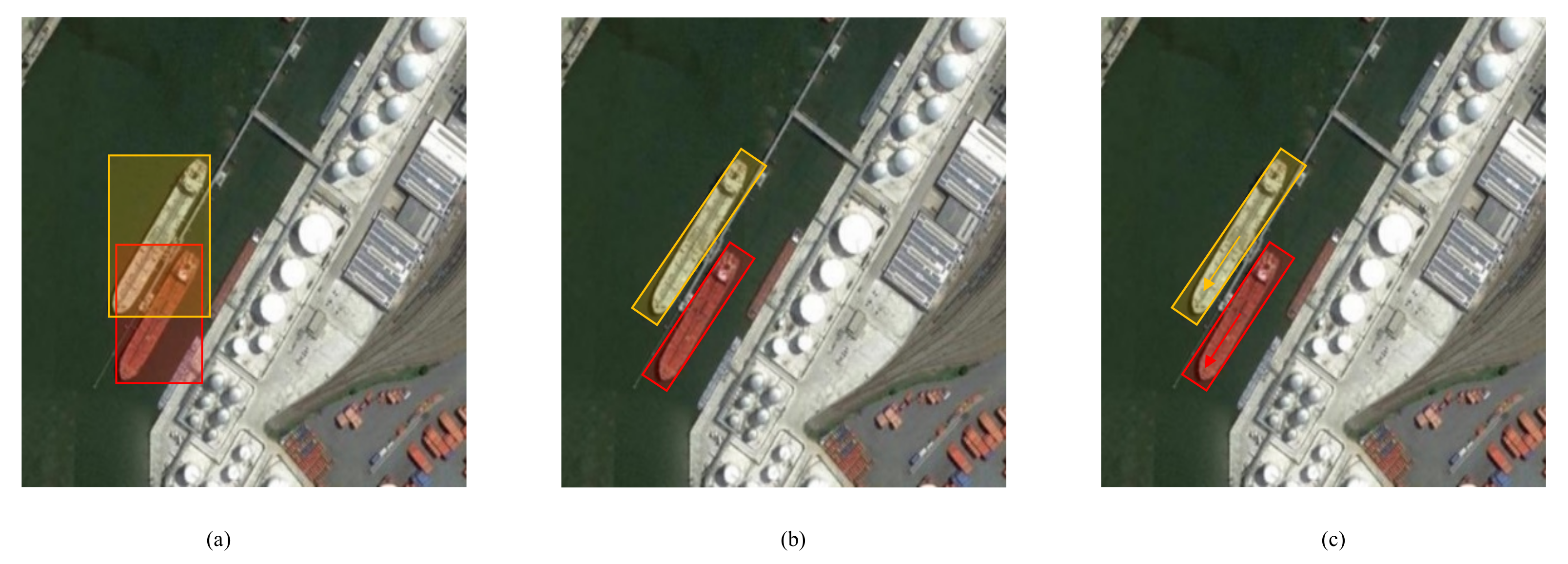
The use of tilted bounding boxes in optical remote sensing images to detect ships has more advantages than the use of horizontal bounding boxes: (1) The ship target is elongated, and the boundary of the tilted bounding box is close to the outline of the ship, avoiding excessive background information to introduce noise; (2) Ship targets are often arranged closely together, and the tilted bounding boxes are marked more clearly to avoid the problem of overlapping labels in horizontal bounding boxes; (3) The tilted bounding boxes can express the orientation information of the ship, which is an important feature of the ship. Tilted bounding boxes can also be subdivided into two categories: rotational bounding box and orientational bounding box. The difference between the rotation bounding box and the orientational bounding box is that the rotation bounding box itself has no direction but only expresses the posture of the rectangle. Rotating around its center still represents the same rotation bounding box; while the orientational bounding box itself has a direction, for example, the arrow in Figure 1c indicates the direction of the tilted bounding box, rotating around its center will indicate another tilted bounding box.
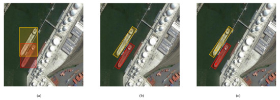
Figure 1.
Three types of representation for object-detection results. (a) Horizontal boxes. (b) Tilted boxes without direction. (c) Tilted boxes with direction.
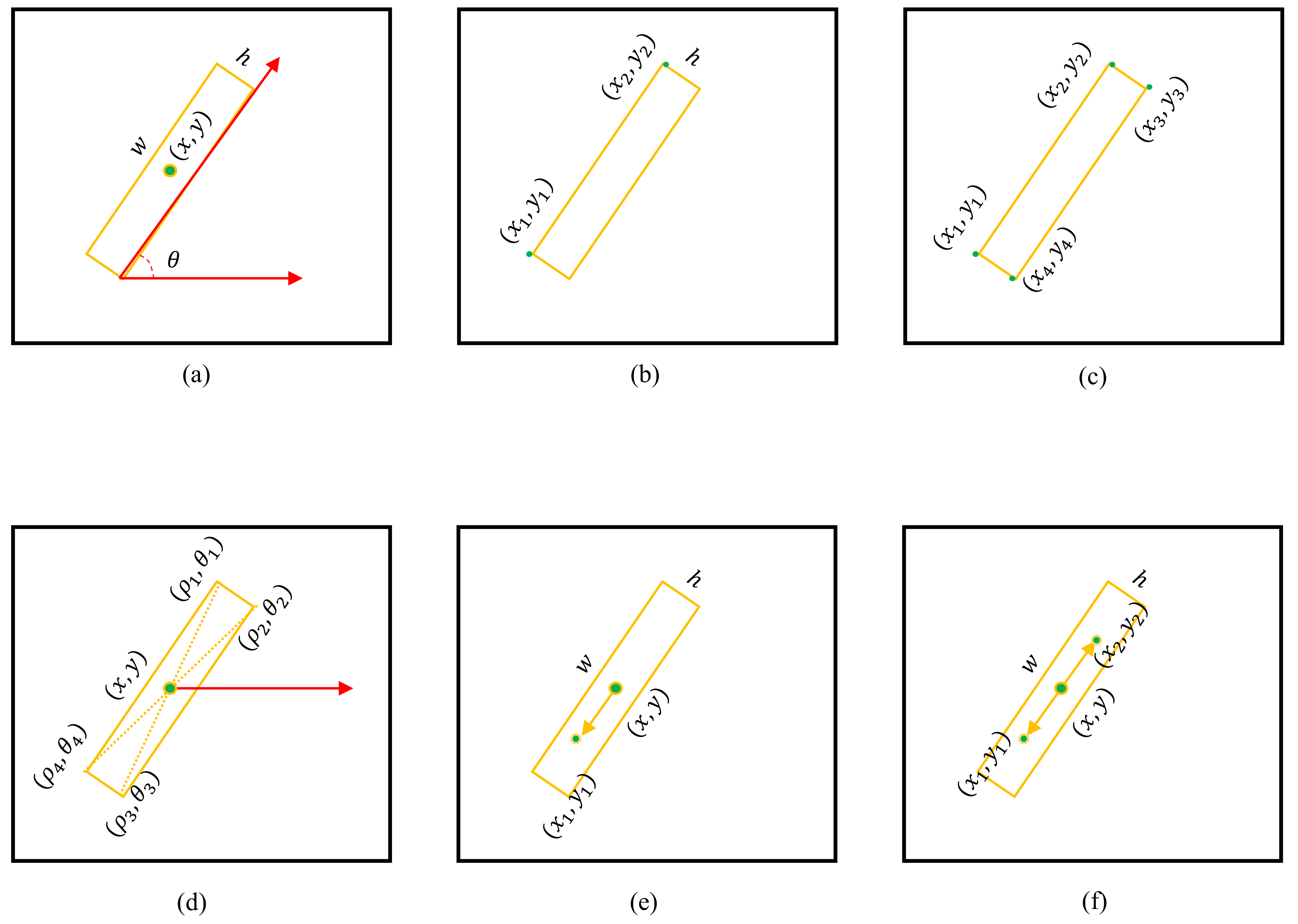
The tilted bounding box needs to indicate the posture or direction of the target, and there are many ways to indicate it. The most common is to use the quintuple to represent an tilted box, as shown in Figure 2a. Literature [36] and Literature [37] both use five-parameter notation, and they agree: represents the geometric center of the box; w and h represent the width and height of the box, respectively; is the long side of the box and the included angle of the x-axis of the image coordinate system is . When the angle is around and the box will be very close, making it difficult for the network to return. SCRDet [38] also uses five-parameter notation, but it adopts the same convention as OpenCV: is still the geometric center of the tilted box; represents the angle of the x-axis positively and counter-clockwise rotated to the first side of the rectangle. This side is defined as w, and the other side is defined as h; then . Under this convention, the ‘first side’ is difficult to parameterize in the neural network, which will bring difficulties to the learning process. The improved five-parameter notation uses , as shown in Figure 2b: and are the two endpoints of one side, and h is the other side’s length. The eight-parameter method directly uses the coordinates of the four vertices of the rectangle to represent an oblique bounding box, as shown in Figure 2c. P-RSDet [39] first predicts the geometric center of the box, and uses as the origin to establish a polar coordinate system. The four vertices of the rectangle are expressed as , as shown in Figure 2d, where , let , then can be expressed as a tilted bounding box. Figure 2e replaces the angle with a direction vector on the basis of (a) to indicate the posture and orientation of the tilted bounding box. If the direction of the ship is specified in the annotation data, this representation method is good; but if the direction of the ship is not specified in the annotation data, the direction vector may point to the bow or the stern of the ship, causing confusion.

Figure 2.
Various representation methods for tilted bounding box. (a) Five parameters. (b) Five parameters. (c) Eight-parameter notation. (d) Center polar coordinate representation. (e) Single direction vector. (f) Tilt dual direction.
This paper proposes a representation method of the tilted bounding box as shown in Figure 2f. is the geometric center of the tilted bounding box. The long and short sides of the tilted bounding box are w and h, and is a unit vector of equal size and opposite direction, then , . In this paper, are called dual direction vectors. When the direction is not specified, the method indicates a rotating tilt bounding box; when the direction is specified, the method indicates a direction tilted bounding box.
A number of anchor-free methods have been proposed in the past several years [30,40,41,42]. CenterNet [30] is a typical and smart anchor-free design for object detection. We choose CenterNet as the basic detection framework and Resnet50 [43] as the basic backbone network for feature extraction. The original CenterNet detection part uses three branches to predict the center point heat map, center offset compensation, and the width and height of the box to output the horizontal detection bounding box. This article adds a fourth branch to it to predict the box pose, as shown in Figure 3. The box pose prediction branch is also composed of a two-layer convolutional network, the number of convolution kernels in the first layer is 256, and the number of convolution kernels in the second layer is 4. Therefore, the number of tensor channels output by the block pose prediction branch is 4, and each channel represents 4 values of the dual direction vector. The improvement of the detection part of CenterNet in this paper enables the neural network to handle both the horizontal bounding box and the tilted bounding box object detection task.
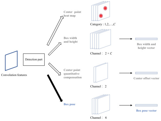
Figure 3.
Improved CenterNet detection part. A box pose prediction branch has been added so that it can predict the tilted bounding box.
3.2. The Structure of the Network Model
From the analysis and research in the previous content, we can know that the convolutional features of the backbone network have different characterization characteristics for ship targets of different scales. The use of fusion features can adjust the object detection performance of various scales, but it is difficult to balance the detection performance of full-scale targets in a single convolution feature. That being the case, why can we not adopt the strategy of “divide and conquer, destroy each” and use suitable convolution features to detect ship targets of different scales? Ship targets in each scale range are detected using the convolution features that best match their characterization characteristics, so that the problem of finding a global optimal solution can be transformed into a problem of finding multiple local optimal solutions.
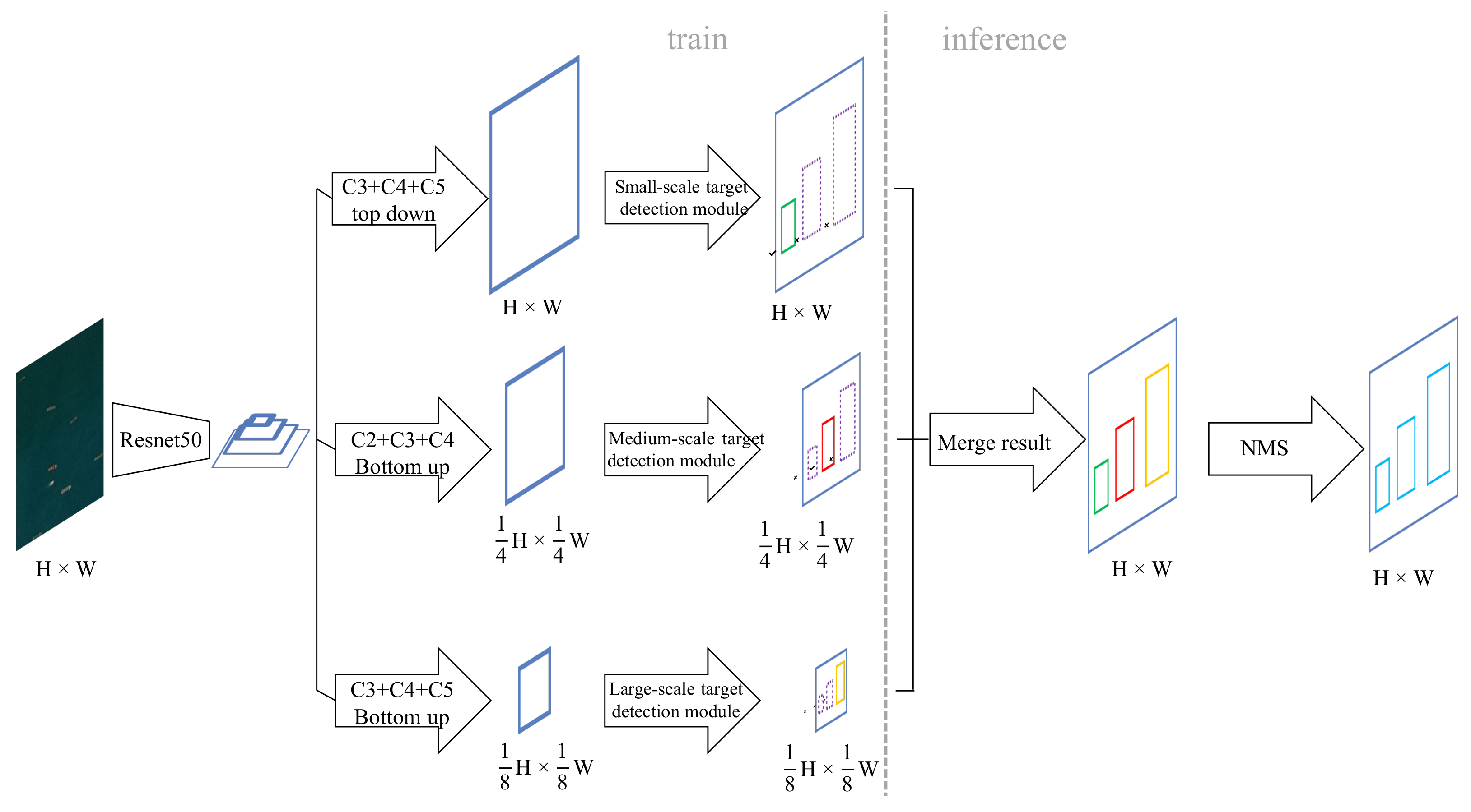
Based on the above ideas, we propose a hierarchical scale sensitive CenterNet (HSSCenterNet) object detection algorithm. The network structure and data flow are shown in Figure 4. The image is input into the feature-extraction network, which obtains four basic features, and Resnet50 is employed as the basic network. Next, the features are passed into three branches, which deal with the ship-detection tasks of small-scale, medium-scale, and large-scale, respectively. For small-scale ship targets, C3, C4, and C5 of the four basic features are selected to fuse along the top-down path, and feature maps are resized to be consistent with the input image to obtain the small-scale fusion feature. Afterwards, the fusion feature is input into the small-scale object detection module, which will only use the fusion features to detect small-scale ship targets. For the medium-scale ship target, C2, C3, C4 features will be selected to fuse along the bottom-up path, and feature maps are resized to of the input image to obtain the medium-scale fusion feature. Similarly, the fusion feature will be processed by the medium-scale object detection module. C3, C4, and C5 features will be fused along a bottom-up path for large-scale ship detection, and the feature maps will be resized to of the input image. The network structure of the detection modules of large, medium, and small scales is the same, and they all use the improved CenterNet detection part, as shown in Figure 3. That is to say, the three detection branches will output the center point heat map, the width and height value of the target box, the center point quantization compensation value, and the dual direction vector of the box, but each branch will only predict the result of the corresponding scale. Then, since the results of the three different scales are predicted based on different convolution feature sizes, they are scaled and merged to the original input image size. Finally, the non-maximum suppression algorithm is used to de-duplicate the combined results to obtain the final detection result.

Figure 4.
An overview of the hierarchical scale sensitive network.
HSSCenterNet is essentially a multi-task network architecture. It decomposes the object detection task into three subtasks: large-scale object detection, medium-scale object detection, and small-scale object detection. Each subtask shares the weight of the basic feature extraction network, and the parameters of each branch network are independent of each other, and the training and inference of the three are not interfering with each other.
3.3. Network Model Training
Let denote the input image, the width is W and the height is H. For ship targets in each scale range, the neural network outputs the center point heat map , center point offset compensation , box size , and the bounding box pose , where represents the small-scale, the medium-scale, and the large-scale, respectively. Assuming that there is a ship target in the training sample image I, the coordinates of the upper left and lower right corners of its box are . Then its center point is , and the coordinate of point p is . Its size is , and s is expressed as .
Center point heat map , where is downsampling rate and C is the number of categories. Here , because there is only one category of ship. The prediction result indicates that the point corresponds to the center of a target box, and indicates the background. For the ship target of each scale in the image I, the center point of the box is p, and the category is . The corresponding point of point p on the center point heat map is . We use Gaussian kernel to spread the center point of the training sample on the heat map Above, , where the standard deviation related to the box size. If the Gaussian distributions of the two center points coincide, take the larger value. We use an improved focal loss supervised neural network to predict the center point heat map, which is an optimized objective function for pixel logistic regression with penalty terms:
where and are the hyperparameters in focal loss, and is the number of target center points with scale ∗ in image I. is used to normalize the focal loss values of the center points of all positive samples of this scale. In this experiment, and are set.
Since the size of the center point heat map is different from the input image, there is a quantitative offset from the predicted coordinates on the center point heat map. The offset compensation of the center point of each target box is . The offset compensation prediction is trained using the L1 loss function:
In the training, the loss value is only calculated for the pixel where the point is located, and other positions are not involved in the calculation. After predicting the center point p of the target box, it is also necessary to predict the width and height of the box, or the size of the box . The dimension of the target box where point p is located is . Similar to the center offset compensation, the optimization goal of the box size is also the L1 loss function:
When predicting the width and height of the box, it will not be regularized or obtained from the center point heat map, but directly return to the size of the target in the coordinate system of the input image. If you perform the task of detecting tilted bounding boxes, you also need to predict the pose of the bounding box , that is, the labeled dual vector of the target box where the point p is located as , and the predicted dual direction vector is . The optimization goal of the tilt bounding box attitude prediction network consists of three parts. The first part is the loss function:
The two vectors, , and , are equal in size and opposite in direction. This constraint is regarded as the second part of the optimization objective ,
and they are also unit vectors at the same time. The third part of the optimization objective is ,
Therefore, the tilt box pose loss function can be formulated as
where the parameters are empirically set as . The network we designed uses three branches to detect targets of different scales. The optimization goal of each detection branch are as follows,
where the parameters are also empirically set in the experiment. As a results, the optimization goal of the entire network is formulated by
Obviously, if there is no restriction, each scale detection branch will be affected by samples of other scales during training. For example, the small object detection branch will calculate the loss value of the large and medium target samples during training, and the small object detection branch will receive the interference from large and medium scale samples when returning the gradient update weight parameter in . The same is true for the medium-scale and large-scale object detection branches.
In order to avoid a single branch from being affected by targets of other scales during training, TridentNet [26] uses the proposed region selection mechanism proposed by SNIP [23]. We also use this mechanism. Assuming that the ship target width and height calculated in the forward direction during training are w and h, respectively, then only when , the gradient of the target sample participates in the reverse calculation. Here and , respectively, represent the upper and lower limits of the effective scale of the scale detection branch. Since SNIP [23] and TridentNet [26] use Faster-RCNN [11] as the basic detection bounding boxwork, it is very convenient and reasonable to use the selection mechanism in RPN and RCNN. When training an RPN, you only need to select a valid sample when the training sample assigns a label to the anchor box. When training RCNN, you only need to select valid samples when the training samples assign labels to the proposed region. However, CenterNet is a single-stage non-anchor bounding box detection bounding boxwork, and it is difficult to screen effective samples as clearly as the anchor bounding box mechanism. The three detection branches of TridentNet are calculated in the same coordinate reference system, and the three detection branches of the HSSCenterNet we designed have been scaled at different sampling rates, which means that the coordinate reference systems calculated by the three are not the same. Therefore, when generating training label data, it is necessary to generate three sets of label data corresponding to the sample sizes of the three detection branches.
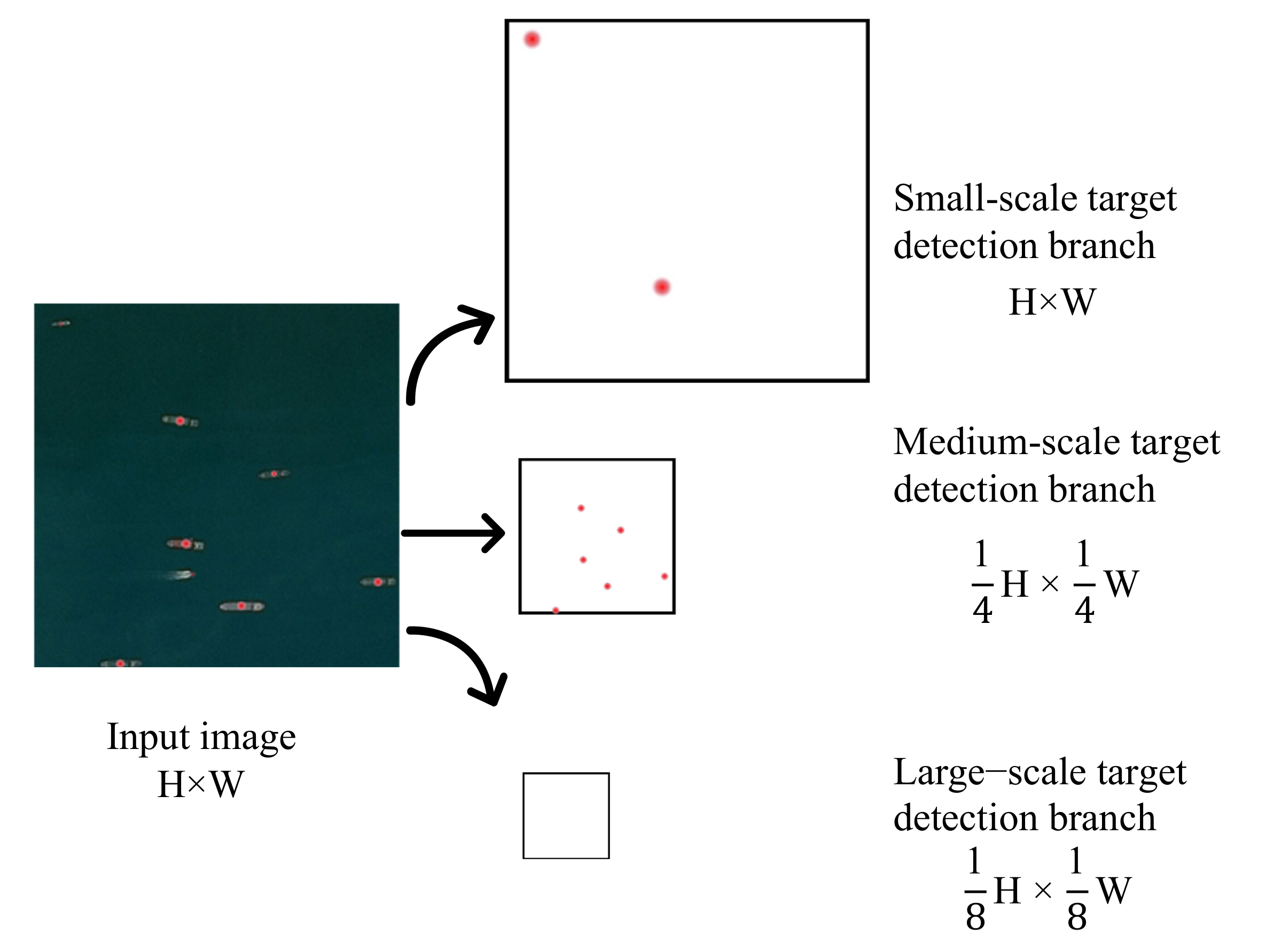
As shown in Figure 5, the input image size is , and there are 3 heat maps at the center of the target box. The size of the heat map corresponding to the center point of the small-scale detection branch is , which only includes the center point distribution of small-scale ships; the size of the center point heat map corresponding to the medium-scale detection branch is , and this map only contains the center point distribution of medium-scale ships; the size of the center point heat map corresponding to the large-scale detection branch is , which only includes the center point distribution of large-scale ships. If the training image does not contain a ship target within the range of a certain detection branch scale, a blank heat map is used instead. For example, the training image in Figure 5 does not contain large-scale ship targets, and the heat map corresponding to the large-scale detection branch is still generated. This is to facilitate the use of larger batch sizes when training the model.
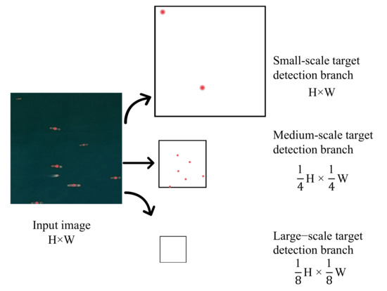
Figure 5.
Heat map of the center point of each branch of the hierarchical scale sensitive network.
As explained in the previous subsection, the standard deviation of the Gaussian distribution on the heat map in the standard CenterNet is , where r is the radius of the distribution circle of the actual label bounding box distribution of the positive sample. The distribution radius r is related to the intersection of the actual labeling bounding box and the distribution of positive samples than the threshold t and the size of the labeling bounding box , , where p represents the center point of the labeling bounding box. Since the size of the convolution feature used for detection of each branch is different, the standard deviation of the two-dimensional Gaussian distribution on the heat map corresponding to the center point of each branch is also different, and the specific settings are as follows:
At the same time, the training data of center point offset and box size should be divided into three groups according to the size. In short, the annotation data of a training image needs to be divided into three parts, corresponding to three detection branches of different scales.
This hierarchical multi-scale training mechanism (HMSTM) can make it possible to distinguish scale differences. From the perspective of the backward calculation process when returning the gradient and updating the weight, the parameters of the small-scale detection branch are only updated by small-scale target samples, and the parameters of the medium-scale detection branch are only updated by the medium-scale target samples. The parameters are only updated by large-scale target samples. When the weight of the basic feature extraction network is updated, its gradient is the sum of the three branch return gradients, which means that the parameters of the basic network are updated by all samples.
3.4. Network Model Testing
The HSSCenterNet inference process we proposed includes all the forward calculation processes in the training phase. That is to say, after the image is input to the network, each branch predicts the heat map of the ship target center point, the center offset compensation tensor, the width and height tensor of the rectangular box, and the posture or direction tensor of the rectangular box within its own scale range. Then, according to the center point coordinates obtained in the center point heat map, the corresponding center offset compensation value, the width and height values of the rectangular bounding box, and the dual direction vector of the rectangular bounding box are found through post-processing. Afterwards, the output of each network branch will be converted into the coordinates of a rectangular box, and all the output will be merged together. Finally, the non-maximum suppression algorithm is used to remove the redundant rectangular bounding box of the target.
4. Experiments and Results
In this section, we first introduce two datsets for ship detection, the evaluation metrics, then introduce the experimental settings, and finally report the ship-detection results.
4.1. Datasets
This study uses two datasets: Airbus ship dataset and WHUCS ship dataset. We introduce each of them in the subsection.
Airbus ship dataset. In order to promote the development of ship detection technology from satellite optical images, Airbus Group has produced the Airbus ship detection dataset and released related competitions on the Kaggle competition platform. The Airbus ship dataset on the Kaggle platform only discloses part of the training set, and we use part of the public dataset for exploratory experiments. The Airbus ship dataset contains a total of 192,556 images, each with a resolution of . In all the images, some do not contain ships, and some contain one or more ships. We divide the Airbus ship dataset into two parts: training set and test set. The training set has a total of 134,789 images, of which 29,789 images contain ships and 105,000 images do not contain ships. A total of 57,767 images in the test set, with 45,000 images not containing ships. The Airbus ship dataset is labeled in the form of binary segmentation [44]. In addition, we follow the definition of the COCO dataset and define ships with a pixel area less than as small targets, ships with a pixel area in the range of to as medium-scale, and ships with a pixel area greater than as large-scale. The details of Airbus ship dataset are shown in Table 1.

Table 1.
Airbus ship dataset.
WHUCS ship dataset. It is a new dataset we collect for ship detection from remote sensing images. The WHUCS ship dataset can be cross-validated with Airbus ship detection. In the WHUCS ship dataset, the training set contains 1,464 images, and the test set contains 200 images, each of which contains multiple ships. In the dataset, the resolution of each image is . The dataset is marked with a tilted box, and the pixel area of the ship is regarded as the area of the target. Additionally, following the definition of COCO dataset, ships are divided into three types: small-scale, medium-scale, and large-scale according to pixel area. The details of WHUCS ship dataset are shown in Table 2. We can see that, the scale of WHUCS ship dataset is smaller than that of Airbus ship dataset. Although some images in Airbus do not contain any ships, each image in WHUCS contains multiple ships.
Table 2.
WHUCS ship dataset.
It is worthwhile to note that we follow the definition of small objects in COCO dataset. There are two reasons: one is that, we treat the small object detection as a common visual perception task, where we only care about the absolute pixel size of the object. In other words, we do not consider the spatial resolution of the image. The other is that, we indeed have difficulties in retrieving the spatial resolution of the images when we construct the dataset.
4.2. Evaluation Metrics
The experiment in this article uses the evaluation method of COCO [45], so that the development tool set COCOAPI provided by the official COCO dataset can be used. In COCOAPI, the mean average precision is used as the main evaluation index. Average precision refers to the average accuracy of all categories under the determined prediction box and the IOU threshold of the labeled box. The average accuracy rate calculation formula is as follows:
where is the threshold of IOU, represents the accuracy of category c in iou>, and C is the number of categories. The average average accuracy rate refers to taking multiple IOU thresholds and calculating the average average accuracy rate under the multiple IOU thresholds. The formula for calculating the average average accuracy rate is as follows:
where K is the number selected by the IOU threshold. We follow the setting of COCO, the threshold of IOU is 0.50:0.05:0.95, from 0.5 to 0.95, every interval is 0.05, so . In this experiment, there is only one category of ships, so the accuracy of one category of ships can be calculated.
In addition, we calculate the average accuracy of small-scale ships, medium-scale ships, and large-scale ships, which are formulated as
For simplicity, in the following text, mAP is abbreviated as AP, is abbreviated as , is abbreviated as , and is abbreviated as .
4.3. Experimental Setup
Training. We implement the HSSCenterNet code based on the PyTorch [46] deep learning bounding boxwork and use the Kamin method [47] to initialize the weight parameters of the deep neural network. Due to the improved focal loss, we follow [48] to set the bias parameters in the convolutional layer to better predict the center point heat map. In the training phase, we use the original image size as the input size. On the Airbus ship detection dataset, the input size is , and the output sizes of the three branches are , , and , respectively. The input size on the WHUCS ship detection dataset is , and the output sizes of the three branches of large, medium, and small are , , and , respectively. In order to reduce model over-fitting, we used common data augmentation techniques, including random horizontal flipping, random scaling and cropping, and random color dithering, where color dithering involves adjusting the brightness, saturation, and contrast of the image. Finally, the image is normalized by Z-Score and then input into the deep neural network.
We use the stochastic gradient descent algorithm (SGD with Momentum) [49] to optimize the network model parameters. The initial learning rate is set to 0.02, the momentum value is 0.09, and the weight decay rate is 0.0001. We use 8 Nvidia GeForce 1080-Ti graphics cards to train the model on a distributed platform. We set the batch size to 32, then the batch size on each graphics card is 4. In order to adapt to train the model on a distributed platform, and enlarge the batch size on a single graphics card, we replace the batch normalization (BN) [50] in the neural network with group normalization (GN) [51]. In order to improve the efficiency of network training, we set up a learning rate decay strategy. On the Airbus ship detection dataset, a total of 300,000 iterations have been run for the model to reach the convergence state. The initial learning rate is used for the first 200,000 iterations; the learning rate for the 200,000 to 250,000 iterations is 0.002, and the 250,000th iteration to the end of training is 0.0002. We use different learning rate decay strategies on the WHUCS ship detection dataset, with total of 100,000 iterations. For the first 20,000 iterations, the initial learning rate is used. After the 20,000th iteration, the learning rate decays to 0.002, and after the 60,000th iterations, the learning rate decays to 0.0002.
Test. In the testing phase, we use a simple post-processing process to convert the heat map tensor, center offset tensor, and box width and height tensor output by each of the three detection branches into box coordinates. First, use a maximum pooling layer for the central heat map to suppress non-maximum values. Next, select the first 100 peaks in the center heat map of each branch, find the corresponding values in the center offset tensor and the box width and height tensor through the coordinates of the peaks, and remove the results that are not in the detection range of the respective branches. If the tilt bounding box is detected, the dual direction vector is also predicted. Assuming that the output of the network is , take as the prediction result. Then, convert the center point of the corresponding box, the center point offset, the width and height of the box into the coordinate value of the box on the original image. The peak at the center point represents the confidence score of the detection as a ship. Finally, the respective results of the three detection branches are combined and the non-maximum suppression algorithm is applied to remove redundant duplicate results, and the first 100 detection bounding boxes are selected as the final detection results of the model according to the confidence level from high to low.
4.4. Validation Experiments
4.4.1. Regression Mechanism of Tilted Bounding Boxes
Table 3 lists the results of the validation experiment on the tilted box regression mechanism. The first line represents the use of horizontal boxes to label the training dual direction vector tilt box regression mechanism. Compared with the horizontal bounding box, the use of the tilted bounding box can significantly improve the average accuracy of the detection task. In the case that dual direction vectors are used as the slanted bounding box regression mechanism, using the tilted bounding box can increase the AP by compared to using the horizontal bounding box. However, the regression mechanism that uses the dual direction vector as the tilted bounding box can improve the detection accuracy than the regression mechanism that uses a single direction vector as the tilted bounding box. Figure 6 shows the sample results of the tilted bounding box ship detection on the test set of Airbus ship dataset.
Table 3.
Validation experiments on the regression mechanism of tilted boxes. -SDV: a sloping box regression mechanism using only a single direction vector; -DDV: a sloping box regression mechanism using dual direction vectors. -H: using the horizontal box label to train the tilted bounding box detection task, that is to say, the angle is fixed at ; -R: using the tilted box label to train the tilted bounding box detection task.

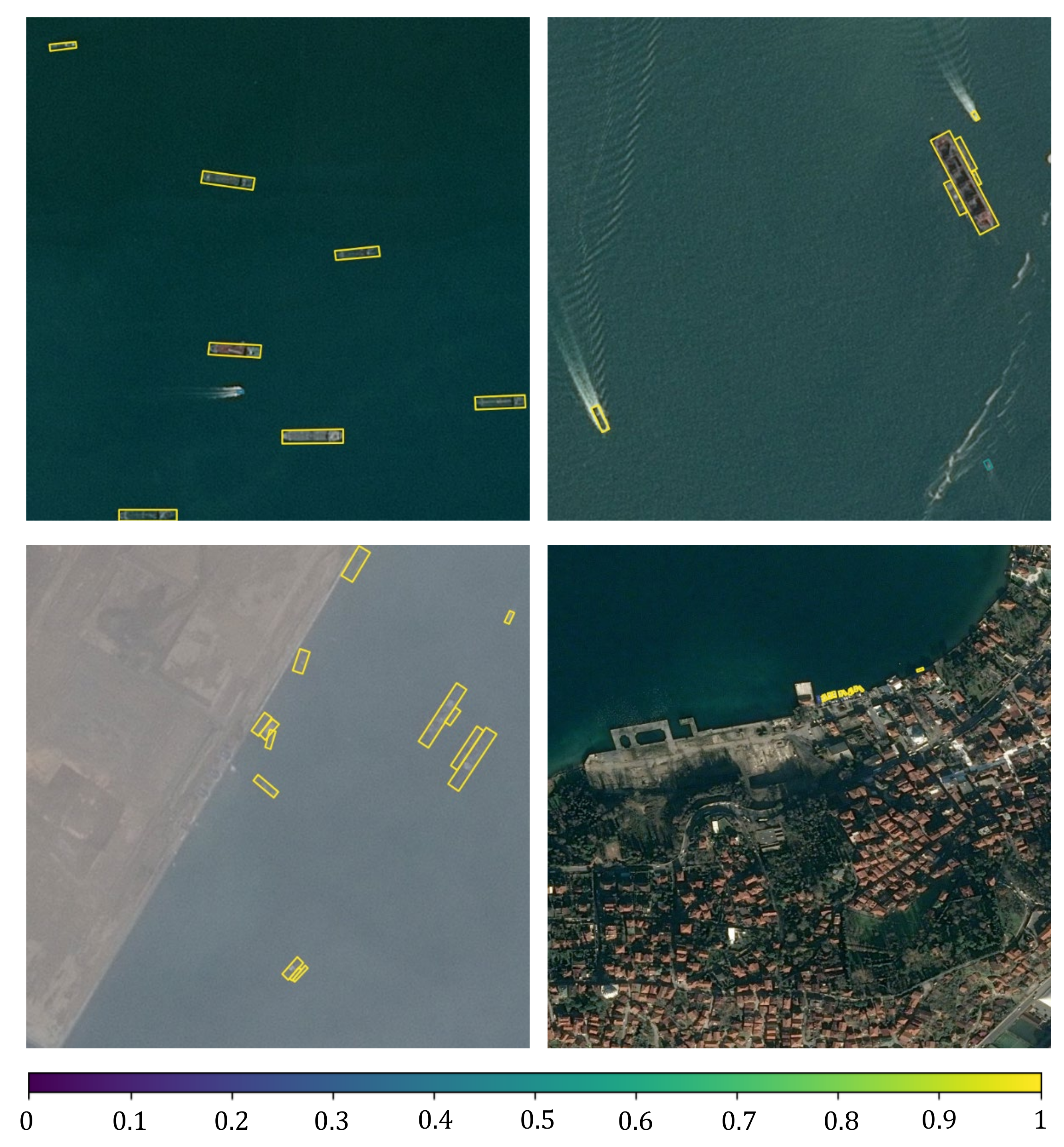
Figure 6.
The detection results in tilted box on the Airbus ship dataset (the color of the detection box indicates its confidence score).
4.4.2. Hierarchical Multi-Scale Training Mechanism
The hierarchical multi-scale training mechanism is the joint link of HSSCenterNet. In order to better understand the importance of the hierarchical multi-scale training mechanism to the network model, we do not use the hierarchical multi-scale training mechanism and train the HSSCenterNet model with the same structure and parameters. In other words, the three detection branches of the additionally trained model all use full-scale samples during training.
Table 4 is the experimental results of exploring the hierarchical multi-scale training mechanism. It can be seen that the hierarchical multi-scale training mechanism can effectively improve the performance of the model, with an increase of on the indicator AP, an increase of on the indicator , and an increase of on the indicator . In addition, hierarchical multi-scale training improves the detection accuracy of small target ships more significantly than that of medium-scale and large-scale targets. The detection accuracy of small targets has increased by , and the detection accuracy of medium-scale and large-scale targets has increased by and , respectively. This is because the separation of training samples of different scales allows the detection branches of different scales to focus on the learning of the feature expression of targets in their respective scales; at the same time, the expression of small target features by the small-scale detection branch is no longer affected by the large-different medium-scale or large-scale targets.
Table 4.
Validation experiments on the hierarchical multi-scale training mechanism (HMSTM).
4.5. Comparison Experiments
4.5.1. Performance on the Airbus Ship Dataset
The proposed HSSCenterNet belongs to a one-stage anchor-free bounding box method. We compare the experimental results of this method with the comparison methods on the horizontal box detection task of the Airbus ship dataset in Table 5. In the one-stage method, the method proposed in this paper is significantly better than the method based on anchor bounding box in all indicators. Compared with the original CenterNet that uses Resnet50 as the backbone network, AP is increased by , is increased by , and is increased by . This is mainly because the detection ability of small targets has been significantly enhanced, has increased by , and the detection performance of medium-scale and large-scale targets has been maintained, has increased by , and has increased by . Even compared with the two-stage method, the HSSCenterNet proposed in this paper is not much inferior. Table 6 compares the hardware overhead of this method with Faster-RCNN and CenterNet. The running speed of this method on a single Nvidia GeForce GTX 1080-Ti graphics card is 28.4 fps, which is more than twice that of Faster-RCNN, while the memory occupation is about the half.
Table 5.
Test results on the Airbus ship dataset.
Table 6.
Running speed and GPU memory capacity when using a single Nvidia GeForce GTX 1080-Ti GPU to test on the Airbus ship dataset.
4.5.2. Performance on WHUCS Ship Dataset
We list the experimental results of HSSCenterNet and other mainstream methods on the horizontal box detection task of the WHUCS ship detection test set in Table 7. The volume of the dataset WHUCS ship detection is very small, and the ratio of the number of ship targets in the three scales of small, medium, and large is about 1:2:1, and their scales vary widely. Therefore, it is difficult for the method without anchor bounding box to detect large-scale ship targets on these data. The accuracy of the anchor-free method for detecting large-scale ships is even lower than that of detecting small-target ships. At the same time, whether it is a one-stage method or a two-stage method, the ratio of the AP of the detection method based on the anchor bounding box to the small, medium, and large ship targets is roughly maintained at about 1:2:2. This also shows the robustness of the anchor bounding box mechanism to large-scale scale changes. Compared with the native CenterNet, the method proposed in this paper not only has higher accuracy, is increased by , is increased by , and is increased by ; it also has an aggressive target scale comparable to the anchor bounding box-based method. The robustness of changes, , , and are , and , respectively.
Table 7.
Comparison of experimental results on the test set of WHUCS ship dataset.
5. Conclusions
In this paper, a hierarchical scale-sensitive network HSSCenterNet was proposed for ship detection from remote sensing images. The multi-scale object detection task was mapped into a multi-task learning problem. To improve the detection accuracy of elongated small object, a ship, a tilted bounding box was proposed, and a dual direction vector was used to express the position and posture. To make full use of the multi-scale features, three detection branches were presented behind the shared basic feature extraction network to detect the small-, medium-, and large-scale ship targets, respectively. A feature fusion sub-network was designed to generate the corresponding fusion feature maps. Meanwhile, a hierarchical multi-scale training mechanism was introduced to improve the scale sensitivity of ship targets during the training process.
Experimental results demonstrated that, the proposed dual direction vector tilted bounding box mechanism effectively improved the average detection accuracy, and the hierarchical multi-scale training mechanism can also significantly improve the detection performance of the proposed HSSCenterNet, especially on small-scale ships. Comparisons with state-of-the-art methods were conducted on the Airbus ship dataset and the WHUCS ship dataset. The results showed that, the proposed HSSCenterNet reached an advanced level in the ship detection, especially on small-scale ship detection.
In our future work, we will further investigate the scale sensitivities in the object-detection deep neural networks. The representation of targets of different scales may affect each other, which will undermine the performance of the detection model. We will make efforts to find a way to minimize this affect, and further improve the performance of small object detection.
Author Contributions
Z.H., L.H., X.Z. and Y.J. contributed significantly to design this study, L.H., W.Z. and Q.Z. contributed significantly to write this manuscript including the figures and tables. Z.H., X.Z. and Y.J. contributed significantly to the discussion of results and manuscript refinement. Q.Z. contributed significantly to lead this research work. All authors have read and agreed to the published version of the manuscript.
Funding
This research was supported partially by the National Natural Science Foundation of China under grant 62071339 and 61872277, National Key R&D Program of China under grant 2020YFC1522703.
Conflicts of Interest
The authors declare no conflict of interest.
References
- Girshick, R.; Donahue, J.; Darrell, T.; Malik, J. Rich Feature Hierarchies for Accurate Object Detection and Semantic Segmentation. In Proceedings of the IEEE Conference on Computer Vision and Pattern Recognition, Columbus, OH, USA, 23–28 June 2014; pp. 580–587. [Google Scholar]
- Huang, X.; Yang, W.; Zhang, H.; Xia, G.S. Automatic ship detection in SAR images using multi-scale heterogeneities and an a contrario decision. Remote Sens. 2015, 7, 7695–7711. [Google Scholar] [CrossRef] [Green Version]
- Yu, J.G.; Xia, G.S.; Deng, J.; Tian, J. Small object detection in forward-looking infrared images with sea clutter using context-driven Bayesian saliency model. Infrared Phys. Technol. 2015, 73, 175–183. [Google Scholar] [CrossRef]
- Gao, F.; Shi, W.; Wang, J.; Yang, E.; Zhou, H. Enhanced feature extraction for ship detection from multi-resolution and multi-scene synthetic aperture radar (SAR) images. Remote Sens. 2019, 11, 2694. [Google Scholar] [CrossRef] [Green Version]
- Fan, Q.; Chen, F.; Cheng, M.; Lou, S.; Xiao, R.; Zhang, B.; Wang, C.; Li, J. Ship detection using a fully convolutional network with compact polarimetric sar images. Remote Sens. 2019, 11, 2171. [Google Scholar] [CrossRef] [Green Version]
- Chen, L.; Shi, W.; Deng, D. Improved YOLOv3 Based on Attention Mechanism for Fast and Accurate Ship Detection in Optical Remote Sensing Images. Remote Sens. 2021, 13, 660. [Google Scholar] [CrossRef]
- Xu, P.; Li, Q.; Zhang, B.; Wu, F.; Zhao, K.; Du, X.; Yang, C.; Zhong, R. On-Board Real-Time Ship Detection in HISEA-1 SAR Images Based on CFAR and Lightweight Deep Learning. Remote Sens. 2021, 13, 1995. [Google Scholar] [CrossRef]
- Kanjir, U.; Greidanus, H.; Ostir, K. Vessel detection and classification from spaceborne optical images: A literature survey. Remote Sens. Environ. 2018, 207, 1–26. [Google Scholar] [CrossRef]
- Wang, Y.; Wang, C.; Zhang, H.; Dong, Y.; Wei, S. A SAR dataset of ship detection for deep learning under complex backgrounds. Remote Sens. 2019, 11, 765. [Google Scholar] [CrossRef] [Green Version]
- Wang, Y.; Wang, C.; Zhang, H.; Dong, Y.; Wei, S. Automatic ship detection based on RetinaNet using multi-resolution Gaofen-3 imagery. Remote Sens. 2019, 11, 531. [Google Scholar] [CrossRef] [Green Version]
- Ren, S.; He, K.; Girshick, R.; Sun, J. Faster R-CNN: Towards Real-Time Object Detection with Region Proposal Networks. In Proceedings of the Advances in Neural Information Processing Systems, Montreal, QC, Canada, 7–12 December 2015; pp. 91–99. [Google Scholar]
- Ding, J.; Xue, N.; Long, Y.; Xia, G.S.; Lu, Q. Learning roi transformer for oriented object detection in aerial images. In Proceedings of the IEEE Conference on Computer Vision and Pattern Recognition, Long Beach, CA, USA, 15–20 June 2019; pp. 2849–2858. [Google Scholar]
- Han, J.; Ding, J.; Xue, N.; Xia, G.S. Redet: A rotation-equivariant detector for aerial object detection. In Proceedings of the IEEE Conference on Computer Vision and Pattern Recognition, Online, 19–25 June 2021. [Google Scholar]
- Shao, Z.; Wang, L.; Wang, Z.; Du, W.; Wu, W. Saliency-aware convolution neural network for ship detection in surveillance video. IEEE Trans. Circuits Syst. Video Technol. 2020, 30, 781–794. [Google Scholar] [CrossRef]
- Chen, L.; Zou, Q.; Pan, Z.; Lai, D.; Zhu, L. Surrounding Vehicle Detection Using an FPGA Panoramic Camera and Deep CNNs. IEEE Trans. Intell. Transp. Syst. 2019, 21, 5110–5122. [Google Scholar] [CrossRef]
- Everingham, M.; Zisserman, A.; Williams, C. The 2005 PASCAL Visual Object Classes Challenge. In Proceedings of the First International Conference on Machine Learning Challenges: Evaluating Predictive Uncertainty Visual Object Classification, and Recognizing Textual Entailment, Southampton, UK, 11 April 2005; pp. 117–176. [Google Scholar]
- Everingham, M.; Eslami, S.A.; Van Gool, L.; Williams, C.K.; Winn, J.; Zisserman, A. The Pascal Visual Object Classes Challenge: A Retrospective. Int. J. Comput. Vis. 2014, 111, 98–136. [Google Scholar] [CrossRef]
- Chen, C.; Liu, M.Y.; Tuzel, O.; Xiao, J. R-CNN for small object detection. In Asian Conference on Computer Vision; Springer: Cham, Switzerland, 2016; pp. 214–230. [Google Scholar]
- Tong, K.; Wu, Y.; Zhou, F. Recent advances in small object detection based on deep learning: A review. Image Vis. Comput. 2020, 97, 103910. [Google Scholar] [CrossRef]
- Chen, L.; Ding, Q.; Zou, Q.; Chen, Z.; Li, L. DenseLightNet: A light-weight vehicle detection network for autonomous driving. IEEE Trans. Ind. Electron. 2020, 67, 10600–10609. [Google Scholar] [CrossRef]
- Lin, T.Y.; Dollar, P.; Girshick, R.; He, K.; Hariharan, B.; Belongie, S. Feature Pyramid Networks for Object Detection. In Proceedings of the IEEE Conference on Computer Vision and Pattern Recognition (CVPR), Honolulu, HI, USA, 21–26 July 2017; pp. 936–944. [Google Scholar]
- Liu, S.; Qi, L.; Qin, H.; Shi, J.; Jia, J. Path Aggregation Network for Instance Segmentation. In Proceedings of the IEEE Conference on Computer Vision and Pattern Recognition, Salt Lake City, UT, USA, 18–22 June 2018; pp. 8759–8768. [Google Scholar]
- Singh, B.; Davis, L.S. An Analysis of Scale Invariance in Object Detection-SNIP. In Proceedings of the IEEE Conference on Computer Vision and Pattern Recognition, Salt Lake City, UT, USA, 18–22 June 2018; pp. 3578–3587. [Google Scholar]
- Singh, B.; Najibi, M.; Sniper, D.L. Efficient Multi-Scale Training. In Proceedings of the Advances in Neural Information Processing Systems, Montréal, QC, Canada, 3–8 December 2018; Volume 31, pp. 9310–9320. [Google Scholar]
- Hu, P.; Ramanan, D. Finding Tiny Faces. In Proceedings of the IEEE Conference on Computer Vision and Pattern Recognition (CVPR), Honolulu, HI, USA, 21–26 July 2017; pp. 1522–1530. [Google Scholar]
- Li, Y.; Chen, Y.; Wang, N.; Zhang, Z. Scale-Aware Trident Networks for Object Detection. In Proceedings of the IEEE/CVF International Conference on Computer Vision (ICCV), Seoul, Korea, 27 October–2 November 2019; pp. 6053–6062. [Google Scholar]
- Bai, Y.; Zhang, Y.; Ding, M.; Ghanem, B. Finding Tiny Faces in the Wild with Generative Adversarial Network. In Proceedings of the IEEE Conference on Computer Vision and Pattern Recognition, Salt Lake City, UT, USA, 18–22 June 2018; pp. 21–30. [Google Scholar]
- Bai, Y.; Ghanem, B. Multi-Branch Fully Convolutional Network for Face Detection. arXiv 2017, arXiv:1707.06330. [Google Scholar]
- Li, J.; Liang, X.; Wei, Y.; Xu, T.; Feng, J.; Yan, S. Perceptual Generative Adversarial Networks for Small Object Detection. In Proceedings of the IEEE Conference on Computer Vision and Pattern Recognition (CVPR), Honolulu, HI, USA, 21–26 July 2017; pp. 1951–1959. [Google Scholar]
- Zhou, X.; Wang, D.; Krähenbühl, P. Objects as points. arXiv 2019, arXiv:1904.07850. [Google Scholar]
- Hu, Z.; Li, Q.; Zhang, Q.; Zou, Q.; Wu, Z. Unsupervised simplification of image hierarchies via evolution analysis in scale-sets framework. IEEE Trans. Image Process. 2017, 26, 2394–2407. [Google Scholar] [CrossRef]
- Hu, Z.; Zhang, Q.; Zou, Q.; Li, Q.; Wu, G. Stepwise evolution analysis of the region-merging segmentation for scale parameterization. IEEE J. Sel. Top. Appl. Earth Obs. Remote Sens. 2018, 11, 2461–2472. [Google Scholar] [CrossRef]
- Dai, J.; Li, Y.; He, K.; Sun, J. R-FCN: Object Detection via Region-based Fully Convolutional Networks. In Proceedings of the Advances in Neural Information Processing Systems, Barcelona, Spain, 5–10 December 2016; pp. 379–387. [Google Scholar]
- Dai, J.; Qi, H.; Xiong, Y.; Li, Y.; Zhang, G.; Hu, H.; Wei, Y. Deformable Convolutional Networks. In Proceedings of the IEEE International Conference on Computer Vision (ICCV), Venice, Italy, 22–29 October 2017; pp. 764–773. [Google Scholar]
- Lin, Y.; Abdelfatah, K.; Zhou, Y.; Fan, X.; Yu, H.; Qian, H.; Wang, S. Co-interest person detection from multiple wearable camera videos. In Proceedings of the IEEE International Conference on Computer Vision, Santiago, Chile, 7–13 December 2015; pp. 4426–4434. [Google Scholar]
- Ma, J.; Shao, W.; Ye, H.; Wang, L.; Wang, H.; Zheng, Y.; Xue, X. Arbitrary-Oriented Scene Text Detection via Rotation Proposals. IEEE Transacitons Multimed. 2018, 20, 3111–3122. [Google Scholar] [CrossRef] [Green Version]
- Jiang, Y.; Zhu, X.; Wang, X.; Yang, S.; Li, W.; Wang, H.; Fu, P.; Luo, Z. R2CNN: Rotational Region CNN for Orientation Robust Scene Text Detection. arXiv 2017, arXiv:1706.09579. [Google Scholar]
- Yang, X.; Yang, J.; Yan, J.; Zhang, Y.; Zhang, T.; Guo, Z.; Sun, X.; Fu, K. SCRDet: Towards More Robust Detection for Small, Cluttered and Rotated Objects. In Proceedings of the IEEE International Conference on Computer Vision, Seoul, Korea, 27 October–3 November 2019; pp. 8231–8240. [Google Scholar]
- Zhou, L.; Wei, H.; Li, H. Objects detection for remote sensing images based on polar coordinates. arXiv 2020, arXiv:2001.02988. [Google Scholar]
- Law, H.; Deng, J. CornerNet: Detecting Objects as Paired Keypoints. In Proceedings of the European Conference on Computer Vision, Munich, Germany, 8–14 September 2018; pp. 765–781. [Google Scholar]
- Law, H.; Teng, Y.; Russakovsky, O.; Deng, J. CornerNet-Lite: Efficient Keypoint Based Object Detection. arXiv 2020, arXiv:1904.08900. [Google Scholar]
- Tian, Z.; Shen, C.; Chen, H.; He, T. FCOS: Fully Convolutional One-Stage Object Detection. In Proceedings of the IEEE International Conference on Computer Vision (ICCV), Seoul, Korea, 27–28 October 2019; pp. 9626–9635. [Google Scholar]
- He, K.; Zhang, X.; Ren, S.; Sun, J. Deep Residual Learning for Image Recognition. In Proceedings of the 2016 IEEE Conference on Computer Vision and Pattern Recognition CVPR, Las Vegas, NV, USA, 27–30 June 2016; pp. 770–778. [Google Scholar]
- Cao, Y.; Ju, L.; Zou, Q.; Qu, C.; Wang, S. A Multichannel Edge-Weighted Centroidal Voronoi Tessellation algorithm for 3D super-alloy image segmentation. In Proceedings of the IEEE Conference on Computer Vision and Pattern Recognition, Colorado Springs, CO, USA, 20–25 June 2011; pp. 17–24. [Google Scholar]
- Lin, T.Y.; Maire, M.; Belongie, S.; Hays, J. Microsoft COCO: Common Objects in Context. In Proceedings of the European Conference on Computer Vision, Zurich, Switzerland, 6–12 September 2014; pp. 740–755. [Google Scholar]
- Paszke, A.; Gross, S.; Massa, F.; Lerer, A.; Bradbury, J.; Chanan, G.; Killeen, T.; Lin, Z.; Gimelshein, N.; Antiga, L.; et al. PyTorch: An Imperative Style, High-Performance Deep Learning Library. In Proceedings of the Advances in Neural Information Processing Systems, Vancouver, BC, Canada, 8–14 December 2019; Volume 32, pp. 8026–8037. [Google Scholar]
- He, K.; Zhang, X.; Ren, S.; Sun, J. Delving Deep into Rectifiers: Surpassing Human-Level Performance on ImageNet Classification. In Proceedings of the IEEE International Conference on Computer Vision (ICCV), Santiago, Chile, 7–13 December 2015; pp. 1026–1034. [Google Scholar]
- Lin, T.Y.; Goyal, P.; Girshick, R.; He, K.; Dollár, P. Focal loss for dense object detection. In Proceedings of the IEEE International Conference on Computer Vision, Venice, Italy, 22–29 October 2017; pp. 2980–2988. [Google Scholar]
- Sutskever, I.; Martens, J.; Dahl, G.; Hinton, G. On the importance of initialization and momentum in deep learning. In Proceedings of the International Conference on Machine Learning, Atlanta, GA, USA, 16–21 June 2013; pp. 1139–1147. [Google Scholar]
- Ioffe, S.; Szegedy, C. Batch Normalization: Accelerating Deep Network Training by Reducing Internal Covariate Shift. In Proceedings of the International Conference on Machine Learning, Lille, France, 6–11 July 2015; pp. 448–456. [Google Scholar]
- Wu, Y.; He, K. Group Normalization. In Proceedings of the European Conference on Computer Vision, Munich, Germany, 8–14 September 2018; pp. 3–19. [Google Scholar]

Publisher’s Note: MDPI stays neutral with regard to jurisdictional claims in published maps and institutional affiliations. |
© 2021 by the authors. Licensee MDPI, Basel, Switzerland. This article is an open access article distributed under the terms and conditions of the Creative Commons Attribution (CC BY) license (https://creativecommons.org/licenses/by/4.0/).