Reliable Crops Classification Using Limited Number of Sentinel-2 and Sentinel-1 Images

Abstract

The study presents the analysis of the possible use of limited number of the Sentinel-2 and Sentinel-1 to check if crop declarations that the EU farmers submit to receive subsidies are true. The declarations used in the research were randomly divided into two independent sets (training and test). Based on the training set, supervised classification of both single images and their combinations was performed using random forest algorithm in SNAP (ESA) and our own Python scripts. A comparative accuracy analysis was performed on the basis of two forms of confusion matrix (full confusion matrix commonly used in remote sensing and binary confusion matrix used in machine learning) and various accuracy metrics (overall accuracy, accuracy, specificity, sensitivity, etc.). The highest overall accuracy (81%) was obtained in the simultaneous classification of multitemporal images (three Sentinel-2 and one Sentinel-1). An unexpectedly high accuracy (79%) was achieved in the classification of one Sentinel-2 image at the end of May 2018. Noteworthy is the fact that the accuracy of the random forest method trained on the entire training set is equal 80% while using the sampling method ca. 50%. Based on the analysis of various accuracy metrics, it can be concluded that the metrics used in machine learning, for example: specificity and accuracy, are always higher then the overall accuracy. These metrics should be used with caution, because unlike the overall accuracy, to calculate these metrics, not only true positives but also false positives are used as positive results, giving the impression of higher accuracy. Correct calculation of overall accuracy values is essential for comparative analyzes. Reporting the mean accuracy value for the classes as overall accuracy gives a false impression of high accuracy. In our case, the difference was 10–16% for the validation data, and 25–45% for the test data.

1. Introduction

Integrated Administration Control System (IACS) was created in the European Union to control direct payment to agriculture. Under common agricultural policy (CAP), direct payments, without going into different payment schemes, apply to crops, which the farmer declares each year, specifying the type of crop (plant) and its area. Some declarations (ca. $5\%$) are controlled using on-the-spot check under which the area of an agricultural parcel is measured and the plant is identified in the field. In order to simplify and automate this procedure, in 2018, the European Commission adopted new rules to control all declared parcels based on Copernicus satellite data: Sentinel-1 (S-1), Sentinel-2 (S-2). In purpose of control farmers’ declarations, the EC research center JRC (Joint Research Center) recommends analysis of time series vegetation indices of any agricultural parcel during the vegetation time [1,2,3].

The most popular index calculated form optical images is NDVI (normalized differential vegetation index) [4] and in microwave spectral range SIGMA (radar backscattering coefficient) [5]. Analysis of the variability plots of these parameters over time allows for reliable assessment of the condition of vegetation and type of crop but it is also work, time consuming and nearly not feasible for all declared plots. There are many initiatives and projects dedicated to agriculture or the CAP (e.g., Sen2Agri, Sen4Cap) among others aimed at the control of direct payments based on the time series of images S-1, S-2.

Automatic image classification for declarations’ inspection seems to be very promising but there are no applicable recommendations for automatic image classification to support audits. The key issue is the credibility of the method as control may result in financial penalties for farmers. Moreover, the verification of all declared parcels is a huge undertaking because it affects areas of the whole country, e.g., in Poland concerns ca. 30% of the country’s area, i.e., 140,000 square kilometers and 10 million agricultural plots.

There are many publications on crops identification in various places around the world, for different purposes and with varying levels of credibility. Analyzing practiced by most researchers methods of image classification for crops recognition, machine learning (ML) undoubtedly dominates: random forest, support vector machine (SVM), convolutional neural network (CNN). The literature reports high accuracies for these methods: e.g., $RF=84.22\%$ [6], $SVM=84.2\%$ [7], $SVM=82.4\%$ [8], $CNN=99.36\%$ [9], $CNN=94.60\%$ [10], $RF=97.85\%$ [11]. A common practice in crops identification is applying the time series consisting of several or several dozen images. Acquiring multiple cloudless S-2 images over a large area is difficult, so many researchers perform analyzes on combinations of a different number of images. In such approaches it is efficient to use cloud computing using ML methods, e.g., Google Earth Engine (some accuracy values reported by the authors: $RF=93.3\%$ [12], $SVMmodified=98.07\%$ [13], $RF=93\%$ [14]).

The level of accuracy achieved with single images is lower, several results can be cited (e.g., [6,7,8]). The accuracy of the classification, using a single S-2 image, of three crops (wheat, sugarcane, fodder), which was performed for the test area located in India, was: $RF=84.22\%$ and $SVM=81.85\%$ [6]. In turn [7], for the test area in Australia, the accuracy of classification of a single S-2 image using the $SVM$ method was 77.4% for annual crops (cotton, rice, maize, canola, wheat, barley) and perennial crops (citrus, almond, cherry, etc.). Especially interesting is [8], where the authors examined the accuracy of the classification of Sentinel-2 images by various classifications methods (RF, SVM, Decision Tree, k-nearest neighbors). They analyzed the results of the S-2 time series for crop recognition in South Africa: canola, lucerne, pasture, wheat and fallow recognition. The highest accuracy was obtained with the use of the support vector machine (SVM) approx. 80%. The most important conclusion is that it was possible to obtain high accuracy of crop classification (77.2%) using single Sentinel-2 image recorded approx. 8 weeks before the harvest. Moreover, they found that adding more than 5 multi-time images does not increase accuracy, and that “good” images do not compensate for “bad” images.

When comparing the research results, the type of crop must be taken into account. The species of cultivated crops depend on the climatic zone in which the research area is located. In this context it is worth citing publications relating to a similar test area to ours. In [15], the authors present the results of research conducted in Northrhinewestfalia (Germany) [15]. They performed a random forest classification of 70 Sentinel-1 mulitemporal images with topographical and cadastral data and reference agricultural parcels obtained from Amtliches Liegenschaftskataster-Informationssystem (ALKIS). With recognition of 11 crops: maize, sugar beet, barley, wheat, rye, spring barley, pasture, rapeseed, potato, pea and carrot very high overall accuracy of $96.7\%$ was obtained (comparing to optic data $91.44\%$).

The other example are the research concerning the IACS system was conducted on the whole area of Belgium [16]. Authors performed an experiment to identify 8 crops: wheat, barley, rapeseed, maize, potatoes, beets, flax and grassland. Various combinations of Sentinel-1 and Sentinel-2 time series were tested in the study. The images were classified using the random forest (RF) method. The maximum accuracy, equal to $82\%$ for the combination of twelve images: six Sentinel-1 and six Sentinel-2 was reported.

The presented two approaches provided high accuracy of crop recognition for control purposes, but required many unclouded images of large areas. This is rather difficult in the case of Sentinel-2, especially considering that the area of Belgium and Northrhinewestfalia is 10 times smaller than the area of Poland.

The similar research were also conducted by our team [17,18]. Ten Sentinel-2 images from September 2016 to August 2017, and nine Sentinel-1 images from March to September 2017 were analyzed. A Spectral Angle Mapper (SAM) classifier was used to classify the time series of NDVI images. Accuracy of $OA$ = 68.27% was achieved, which is consistent with the accuracy (69%) of other independent studies of similar nature conducted in Poland [19]. Therefore, instead of NDVI and SIGMA time series, it was decided to check the possibility of using the classification of single S-2 images and a combination of several multitemporal S-2 images. The aim of the research was to develop a simple, fast but reliable screening method for farmers’ declarations control.

However, while reviewing the literature on the currently used image classification methods for the purpose of crop recognition, we encountered the problem of comparing the accuracy of the classification result. In a traditional remote sensing approach, accuracy is calculated from test data independent of the training data. In machine learning, a lot of attention is paid to the selection of hyperparameters, which is carried out iteratively using only a part of the training set. At the same time, the validation accuracy is determined on the basis of the samples from training set not used for learning.

Some authors report validation accuracy and accuracy calculated on independent test data [7,12,20]. Others only provide information on accuracy based on external reference data not included in the training set [8,15,16,21]. In some publications, there is not enough information on this issue [13,22,23].

There are plenty examples of using only one reference set divided randomly or stratified on training and validation sample, while the distinction between training, validation and independent test data is extremely rare [24].

It turns out that the problem was also noticed by other researchers, e.g., a key work on rigorous accuracy assessment of land cover products [25]. Good practice in accuracy assessment, sampling design for training, validation and accuracy analysis was discussed. The key, from the point of view of our research is the statement: “Using the same data for training and validation can lead to optimistically biased accuracy assessments. Consequently, the training sample and the validation sample need to be independent of each other which can be achieved by appropriately dividing a single sample of reference data or, perhaps more commonly, by acquiring separate samples for training and testing”. Similar conclusions can be found in [26].

Reliability of the classification also depends on the reported accuracy metrics and the unambiguous way of their calculation. Like the previous topic, it is not a trivial issue, although it seems that. Despite many years of research on various accuracy metrics [27,28,29,30,31,32,33] in the 2019 paper, mentioned above, it was stated that overall accuracy ($OA$), producer accuracy (PA) and user accuracy (UA) are still considered the basic ones [25].

Unfortunately, the situation in this area has become more complicated due to the common use of ML methods. In recent years, additional accuracy metrics have been developed that are not used in traditional approaches, i.e., specificity and precision. Other metrics calculated automatically in ML tools: sensitivity and precision, correspond, respectively, to producer accuracy (PA) and user accuracy (UA) in traditional image classification.

In extensive reviews of the literature from the past and the latest, comparative analyzes of plenty various metrics can be found [26,27,28,29,30,31,32,33], but they do not respect sensitivity and accuracy, despite they are commonly used in ML. It is worth noting that sensitivity and accuracy are appropriate for the classification of one class. A problem arises when they are used in assessing the classification of multiple classes, especially if the average value of the accuracy [34] or global precision [35] is reported as $OA$, creating an illusion of higher accuracy [36].

Summarizing the issue of the reliability of the classification result, especially using ignorantly ML tools, there is a double risk of overestimation accuracy: related to the lack of independent test set and the incorrect calculation of the most frequently compared metric in the research: $OA$. Therefore, the accuracy of the classification, which has a very significant impact on the reliability and validity of the remote sensing method for verifying the accuracy of the crops declared by farmers, should be demonstrated with deep attention and carefulness. In the article, we focused on three issues:

1.

Image classification in the aspect of screening method of controlling farmers’ declaration based on a limited number of images (verification in Polish conditions of the hypothesis from the publication [8]).

2.

Analysis of the classification’ results made using extremely different sampling design (we did not focus on the description of the model fitting).

3.

Comparing the traditional accuracy metrics with those used in ML (also discussing incorrect $OA$ calculations), in order to confirm the hypothesis about artificially overestimating the accuracy of the classification result.

To the best of our knowledge, there are no publications on a quick and reliable screening method to control the declarations submitted by millions of farmers in each EU country each year. In addition, despite there are some publications [7,25] containing information on artificially overestimating the accuracy of the classification if the $OA$ calculated from the validation set, instead of the test set, but there is no broader discussion of this issue. On the other hand, the issue of incorrect calculation of $OA$ is completely ignored in publications.

2. Materials and Methods

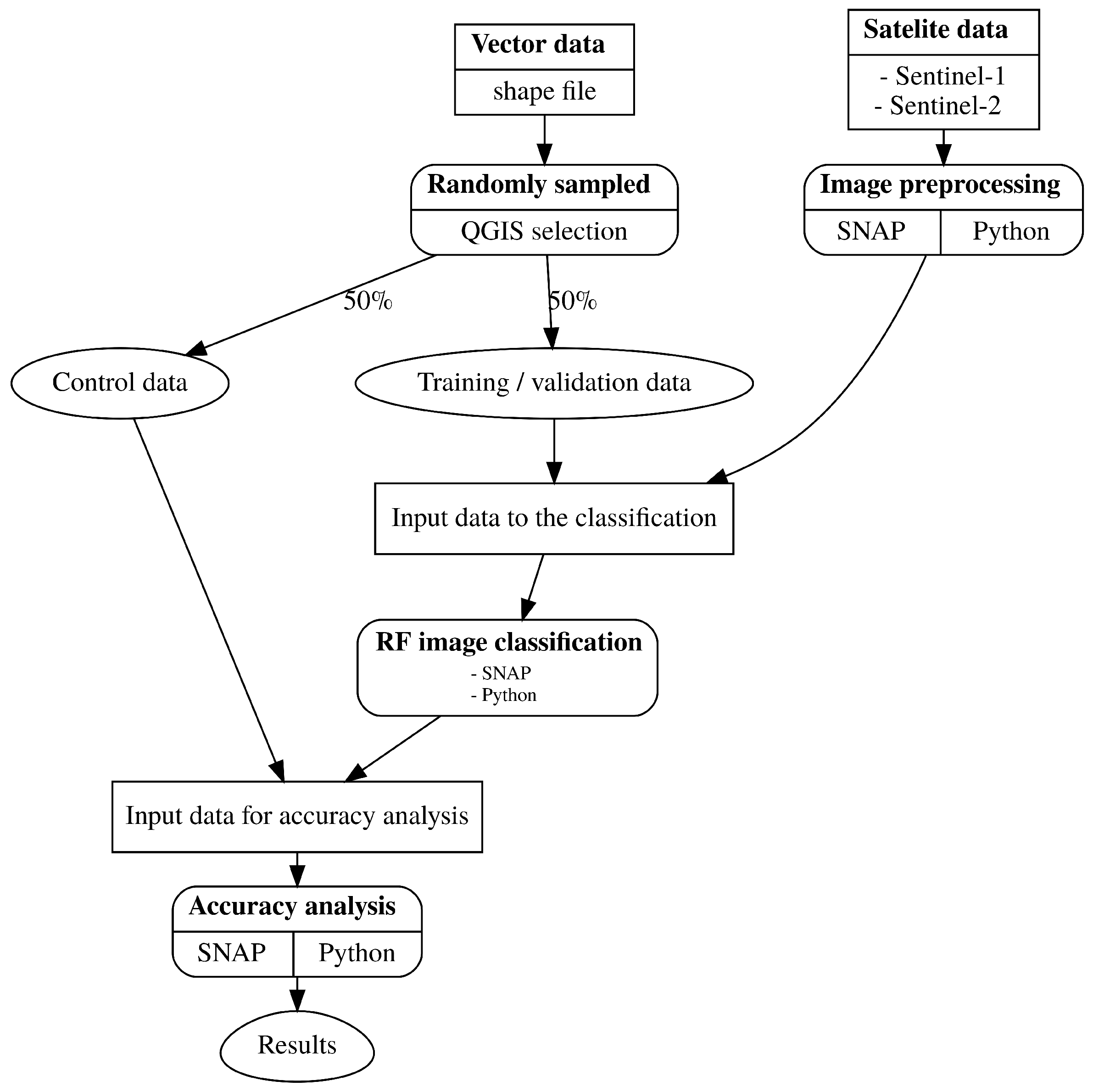
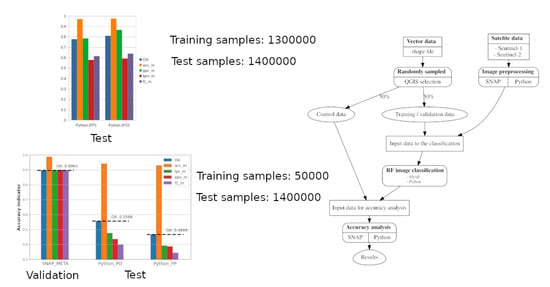
The research consists of three parts Figure 1:

• obtaining and preparing reference and image data,
• image classification,
• comparative accuracy analysis.

2.1. Materials and Data Preparation

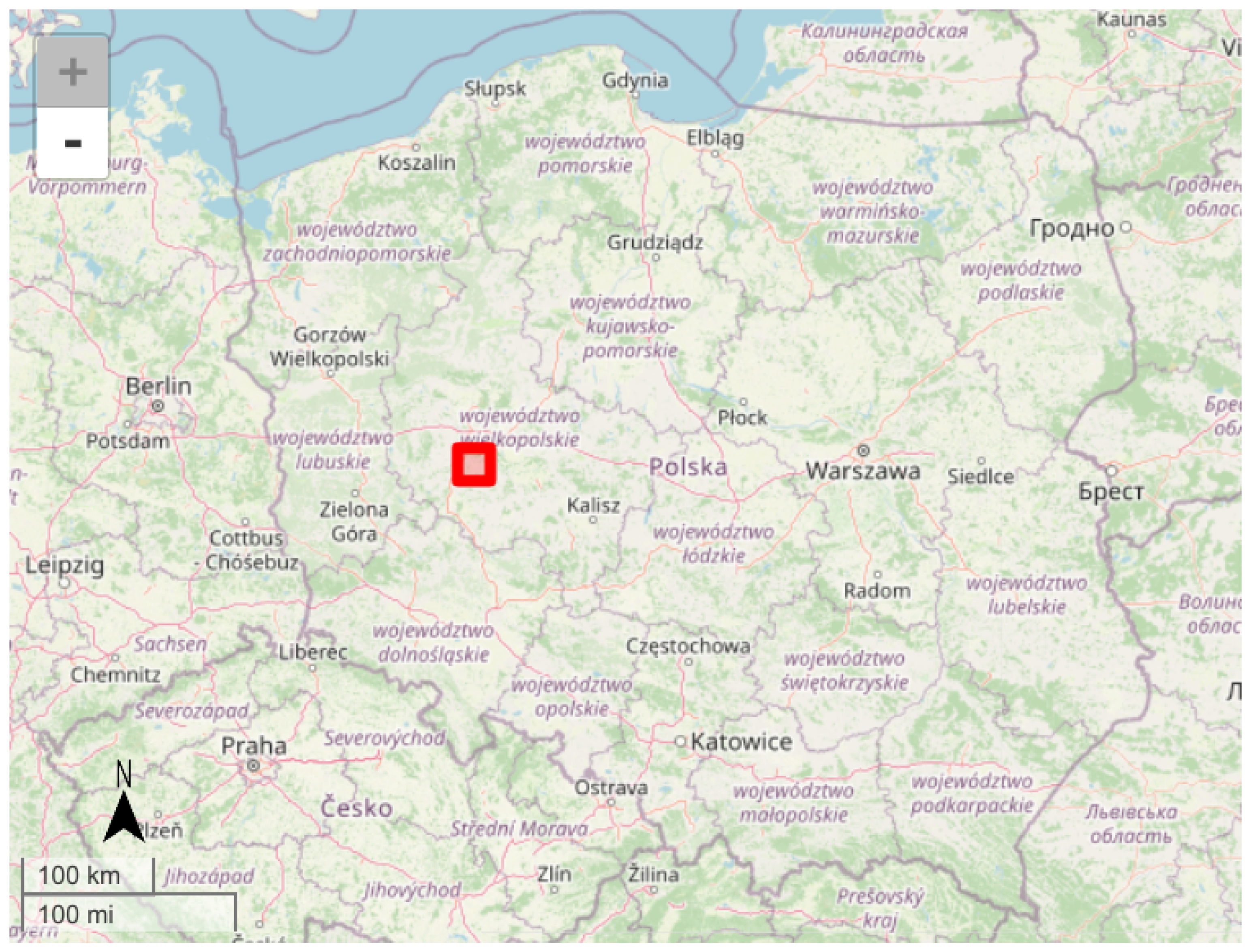
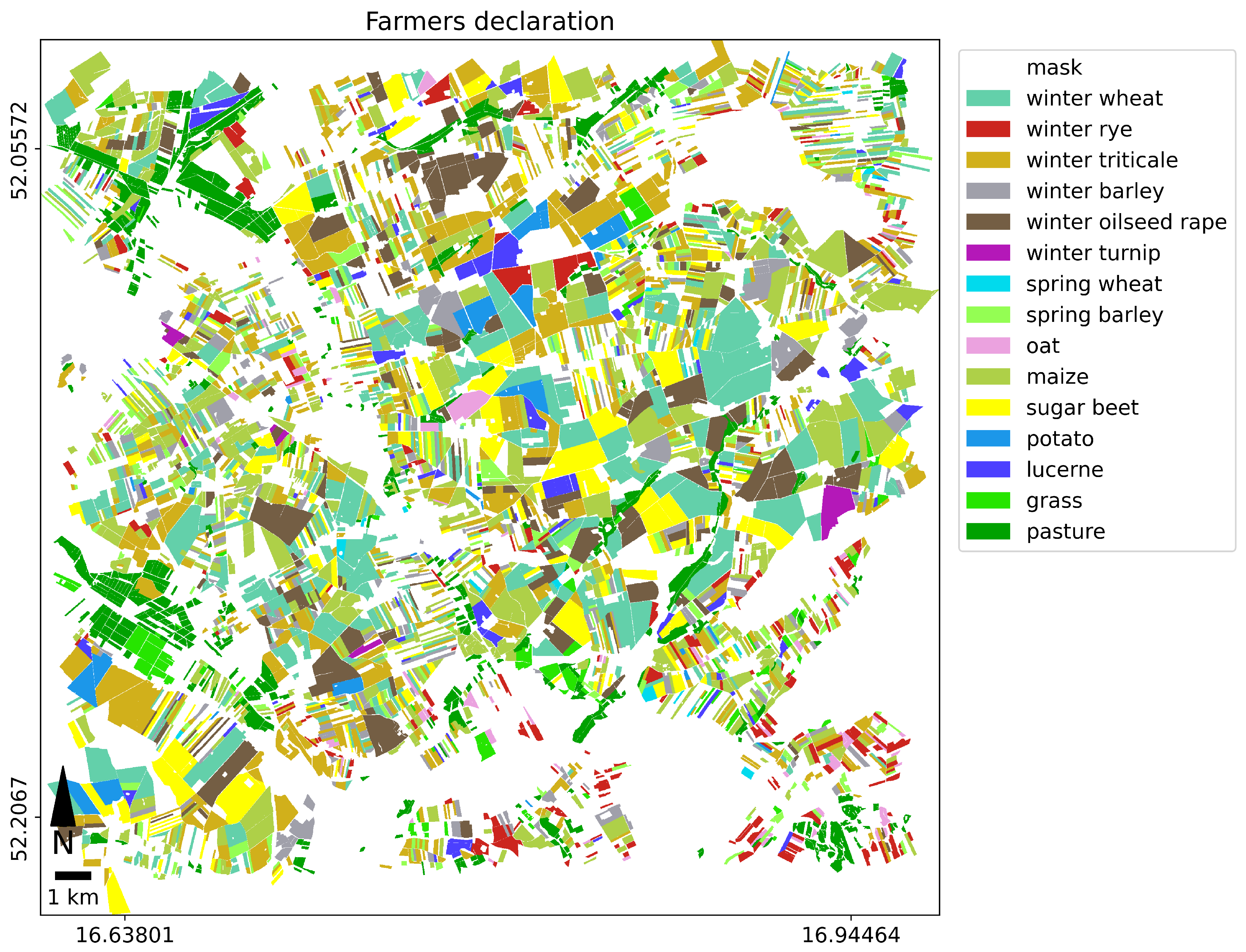
The test area of 625 square kilometers (25 km × 25 km) was located in central Poland, near Poznań (Figure 2), and included 5500 agriculture parcels declared by farmers for the subsidies. Data on farmers’ declarations were provided by Agency for Restructuring and Modernisation of Agriculture (ARMA) in Poland and included size of the agricultural parcel, type of crop, geometry of the agricultural parcel (polygon). The critical size of the agricultural plot is 0.5 ha (this size should exclude the influence of the shape [1]). We selected parcels of the area of 1ha or bigger to avoid technical problems with identifying small parcels. In order to reduce the number of plots and eliminate errors, farmers’ declarations were statistically analyzed for:

• plot size (less than 1 ha),
• use of rare crops (less than 5 declarations).

Finally, 4576 parcels for the analysis were selected (Figure 3,

Table 1. Crops declared for agriculture parcels (area in [ha]).

Id	Crop	Count_Control	Area_Control	Count_Test	Area_Test
1	winter wheat	288	23,749	279	23,754
2	winter rye	117	4389	137	5617
3	winter triticale	402	22,998	452	22,493
4	winter barley	147	6377	178	8652
5	winter oilseed rape	121	10,564	119	15,126
6	winter turnip	3	251	5	1188
7	spring wheat	8	310	11	466
8	spring barley	141	5423	122	3883
9	oat	32	1100	51	2163
10	maize	402	25,213	447	23,961
11	sugar beet	120	11,289	125	11,194
12	potato	11	1059	22	4128
13	lucerne	53	3206	48	2925
14	grass	54	2969	62	2834
15	pasture	291	12,352	328	12,870
	Total	2190	131,250	2386	141,253

).

The parcels’ set was randomly divided into 2 groups: training fields (2190 parcels) and test fields (2386 parcels), which were used for classification and accuracy assessment.

Images from Sentinel-2 and Sentinel-1 satellites of the European Copernicus program (ESA, 2020) were used for the analysis.

Table 2. Characteristics of the Sentinel-2 satellite images.

Parameter	Information
Satellite:	Sentinel-2
Level:	2A (after geometric, radiometric and atmospheric correction)
Selected bands:	10 bands: B2, B3, B4, B5, B6, B7, B8, B8a, B11, B12
Number of images:	3
Dates:	28 September 2017, 26 May 2018, 20 July 2018
Images:
	S2A_MSIL2A_20170928T100021_N9999_R122_T33UXT_20200104T144027
	S2A_MSIL2A_20180526T100031_N0208_R122_T33UXT_20180526T161700
	S2B_MSIL2A_20180720T100029_N0208_R122_T33UXT_20180720T142656
Short name:	S2_20170928, S2_20180526, S2_20180720

and

Table 3. Characteristics of the Sentinel-1 satellite image.

Parameter	Information
Satellite:	Sentinel-1
Level:	Ground Range Detected
Polarisation:	Dual VV+VH
Number of images:	1
Dates:	15 July 2018
Images:
	S1B_IW_GRDH_1SDV_20180715T164255_20180715T164320_011824_015C28_07F3
Short name:	S1_VV_20180715, S1_VH_20180715

contain a list and description of satellite images used in the study. The images were downloaded from the Copernicus Services Data Hub (CSDH) (https://cophub.copernicus.eu/ (accessed on 1 September 2018)).

The data were collected as granules with a size of 100 per 100 km. Three Sentinel-2 images registered in September 2017, May 2018 and July 2018 were selected for analysis. Images of Level-2A were acquired, which means after geometric, radiometric, and atmospheric correction.

Additionally, one Sentinel-1 image was included in the tests, which had been pre-processed for the sigma coefficient, according to the following workflow for two polarization modes (VV and HV):

• radiometric transformation of pixel value to backscatter coefficient (sigma0),
• geometric transformation by Range Doppler orthorectification method with SRTM 3 sek as DEM and bilinear interpolation,
• removing the salt pepper effect called speckle effect using refined Lee filter,
• logarithmic transformation of backscatter coefficient to dB.

In the next step, the classifications were performed on the basis of the following image sets:

• 3 single Sentinel-2,
• 1 combination of 3 Sentinel-2,
• 2 combinations of 4 images: 3 Sentinel-2 and one Sentinel-1 (VV), 3 Sentinel-2 and one Sentinel-1 (HV).

In the single classification, all 10 channels were used, while the channels with a resolution of 20 m were previously resampled to a spatial resolution of 10 m. The classification of the combination of 3 images consists of the classification of 30 channels, 10 from each Sentinel-2 image. The simultaneous classification of optical and radar images was based on the classification of a stack of 31 channels: 30 optical, Sentinel-2 and 1 Sentinel-1 (VV or HV).

2.2. Images’ Classifications

The idea was to use SNAP (ESA) software, because it is open-source commonly used for image processing Sentinel-1, Sentinel-2 and is likely to be used in IACS control. However, it has limitations in the size of the training set. Therefore we prepare our own Python scripts to complete the research.

Eventually, images’ classifications have been carried out with the random forest algorithm using:

• SANP ESA version 8.0.0,
• Python version 3.9.0, scikit-learn version 0.23.2.

As mentioned above, classification in SNAP has some limitations. For example, it is not possible to load a relatively large number of training fields, as in our case (2386 parcels). In addition, the choice of classification parameters, such as, e.g., the number of sample pixels is also limited. The training fields must allow the selection of the required number of training pixels. The total number of assigned sample pixels is divided into the number of classes and from each class the algorithm tries to select this number of pixels if possible. It may be problematic to put the number of sample pixels exceeding the total number of pixels in the class. Therefore, the default settings in SNAP are 5000 sample pixels (due to the sampling method of the training set) and 10 trees (due to the computation time). As part of the research, many different variants of classification with different settings were carried out, especially since the default values were insufficient. The commonly used a grid of parameter method was used to select the best hyper parameters of RF. The GridSearchCV class implemented in scikit-learn was applied. The investigated parameter grid included:

• number of trees in the forest (n_estimators), the range of values: 30, 50, 100, 150, 500,
• the maximum depth of tree (max_depth), the range of values: None, 10, 30, 60, 100,
• the minimum number of samples required to split a node, (min_samples_split), the range of values: 2, 4, 6, 8, 10,
• the minimum number of samples that must be in a leaf node, (min_samples_leaf), the range of values: 1, 2, 4, 6, 8,
• the number of features to consider when split a node, (max_features), the range of values: None, auto,
• bootstrap, the range of values: True, False.

Five k-fold (CV = 5) cross validation was aplied. Three metrics were used to assess the quality of the model: accuracy, mean value of recall (balanced_accuracy), a weighted average of the precision and recall (f1_weighted). In all hyper parameter estimation simulations, all 3 metrics assessed the parameters at the same level. Usually, the set of hyper parameters is selected that best suits the computational capabilities. By increasing the number of trees, you can achieve better results, but it is very limited by the size of the available RAM. Moreover, by increasing the number of trees above 100, the differences in accuracy for the considered problems are negligible, in the order of tenths of a percent (mean_accuracy: 0.8150, 0.8164 i 0.8177, respectively, 50, 100 i 500 trees).

Eventually, a possible large number of sample pixels and trees were assumed:

• 50,000 randomly selected samples (pixels) from the training set,
• 23 number of trees.

There are no such limitations generally in Python, and the whole training set (2190 parcels, 1,412,092 pixels) was possible to use for training. We tested different settings with the k-fold cross-validations and decided to apply the following settings:

• classification: scikit-learn library, sklearn.ensemble module, RandomForestClassifier,
• number of trees: 100,
• min_samples_split’: 2,
• min_samples_lef: 2,
• bootstrap: True,
• max_depth: None,
• max_features: None.

2.3. Accuracy Analysis

Based on a literature review, main metrics were selected for the analysis: $OA,PA,UA$, additionally $f1$ and two metrics from ML, usually not used in remote sensing: accuracy and specificity (

Table 4. Selected accuracy indicators calculated for each class separately except $OA$ [30,38].

RS	Description RS	ML	Description ML	Formula
$OA$	overall accuracy	-	% correct predictions	$OA=\frac{{\sum }_{i=1}^{n}T{P}_i}{{\sum }_{i=1}^n(T{P}_i+T{N}_i+F{P}_i+F{N}_i)}$
-	-	$acc$	accuracy	$acc=\frac{TP+TN}{TP+TN+FP+FN}$
$PA$	producer accuracy	$tpr$	sensitivity	$tpr=\frac{TP}{TP+FN}$
$UA$	user accuracy, reliability	$ppv$	precision	$ppv=\frac{TP}{TP+FP}$
-	-	$tnr$	specificity, true negative rate	$tnr=\frac{TN}{TN+FP}$
-	-	$f1$	F1 score	$f1=\frac{2·TP}{2·TP+FP+FN}$

, please notice difference between $OA$ and accuracy). The meaning of these metrics can be illustrated on any full cross matrix, for example (

Table 5. Example of full confusion matrix (source: [37], Table 4 modified for our purposes—transposed, symbols of classes instead names).

Predicted/True	C1	C2	C3	C4	C5	C6	PA
C1	87	3	0	0	7	0	0.8969
C2	3	90	2	1	0	0	0.9375
C3	0	6	45	0	0	0	0.8823
C4	0	1	0	29	3	0	0.8787
C5	0	2	0	0	23	1	0.8846
C6	0	0	0	1	2	14	0.8235
UA	0.9667	0.8824	0.9574	0.9355	0.6571	0.9333

) taken from the publication from 2021 [37] (it is Table 4—transposed for our purposes).

Accuracy of the classification results is estimated on the basis of the confusion matrix: a full confusion matrix, typically implemented in remote sensing or from a binary confusion matrix used in machine learning.

Full confusion matrix represents the complete error matrix (Table 5), i.e., the combination of all classes with each other using the peer-to-peer method, which includes all commission and omission errors for each class.

Binary confusion matrix contains only cumulative information: number of samples correctly classified as a given class (TP true positives), correctly not classified as this class (TN true negatives), falsely classified as this class (FP false positives) and falsely not classified as this class (FN false negatives). One binary confusion matrix is assigned to one class (e.g., for C1

Table 6. Binary confusion matrix for class C1.

TP	FP		87	3
FN	TN		10	220

). In our case we therefore have 6 binary confusion matrices (

Table 7. Binary confusion matrix for all classes, with metrics.

Class	TP	TN	FP	FN	tpr	trn	acc	ppv	f1
C1	87	220	3	10	0.8969	0.9865	0.9594	0.9667	0.9305
C2	90	212	12	6	0.9375	0.9464	0.9438	0.8824	0.9091
C3	45	267	2	6	0.8824	0.9926	0.975	0.9574	0.9184
C4	29	285	2	4	0.8788	0.993	0.9813	0.9355	0.9063
C5	23	282	12	3	0.8846	0.9592	0.9531	0.6571	0.7541
C6	14	302	1	3	0.8235	0.9967	0.9875	0.9333	0.875
average					0.8839	0.9791	0.9667	0.8887	0.8822

) which are flattened and each matrix written on one row.

From the complete confusion matrix, the binary confusion matrices can be computed, but the reverse operation is impossible.

From both matrices it is possible to compute all metrics and their values are of course the same. However, it should be also noted that there is more information in the full confusion matrix than in the binary confusion matrix. In the case of more than 4 classes, the size of full confusion matrix is larger then size of binary confusion matrix, because the binary confusion matrix for one class is always 2 × 2 (Table 6), after flattering one row in (Table 7). The main advantage of the full confusion matrix is the possibility of exhausting analysis of testing samples and errors (so-called omission and commission errors).

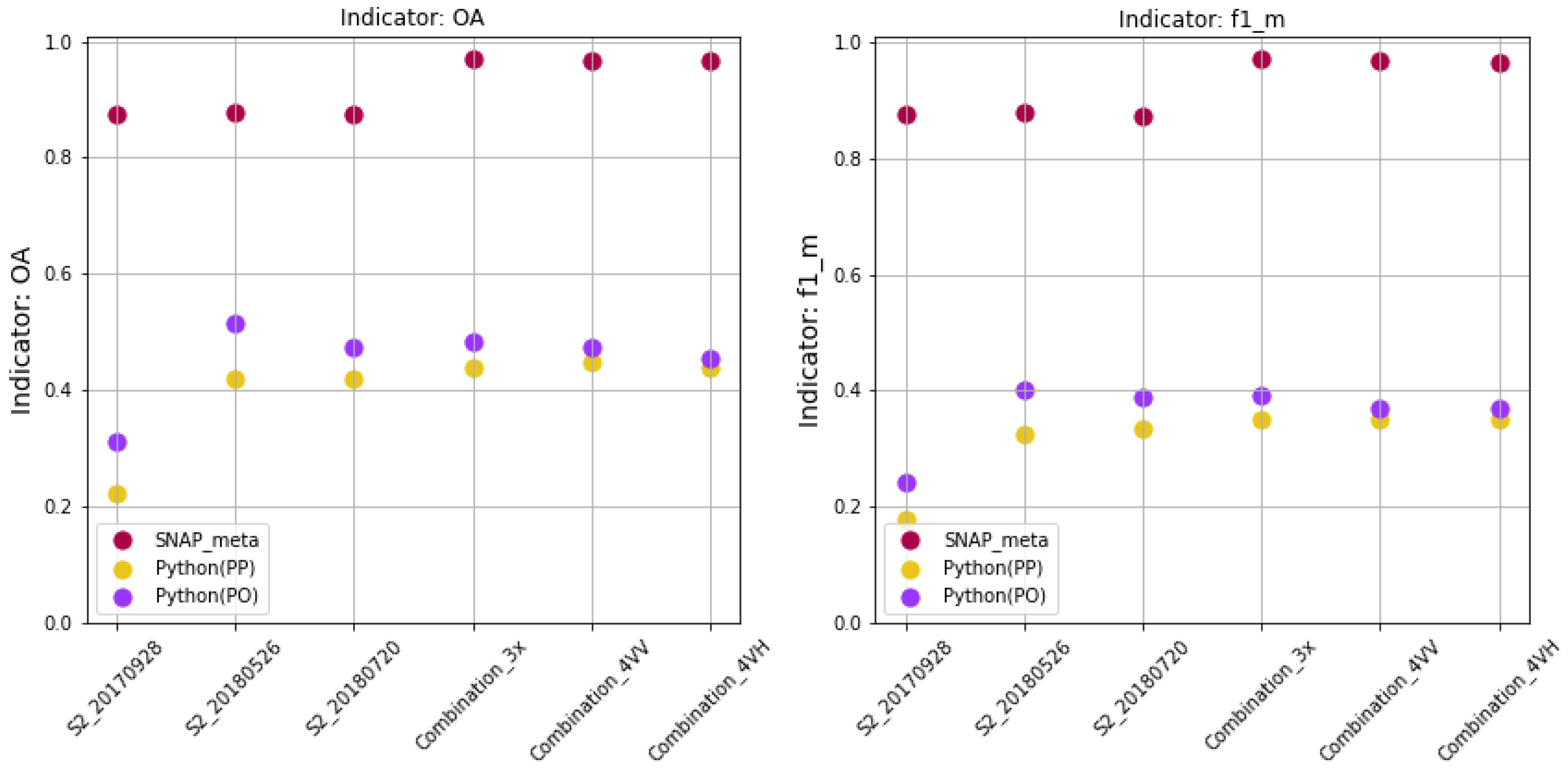
More important, however, is the distinction between $OA$ and the mean value of accuracy ($acc$). The sum of the number of correctly classified samples is used in the numerator to calculate $OA$. In the classification of many classes it is the sum of TP. For one class, we are dealing with samples correctly classified as a given class and correctly not classified to it, i.e., on the diagonal of the binary confusion matrix there is the sum of TP and TN. So, for class C1, $OA$ and $acc$ are equal to (87 + 220)/(87 + 3 + 10 + 220) = 0.9594.

Analyzing individual classes separately, the $acc$ values correspond to $OA$. While the metrics $OA$ for all classes is 0.9000 and is not the mean $acc$ of the classes, which is 0.9667. In this case, the difference is ca. 7% but one should also take into account the relatively small number of TN, because as can be seen from the formula $acc$, the more TN the greater the accuracy ($acc$).

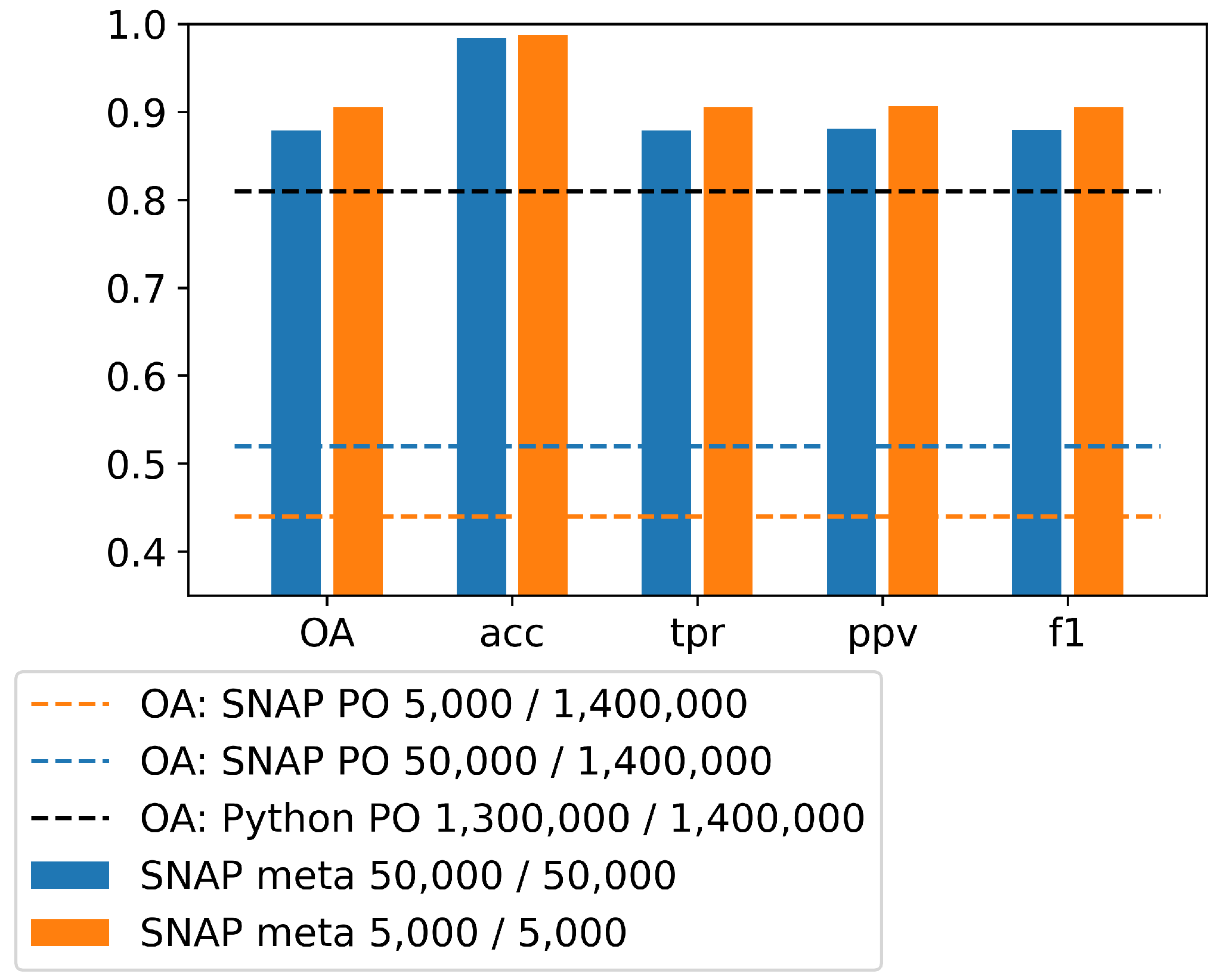
In our research, the accuracy analysis was performed adequately to the classification design. In the case of learning on a selected number of samples, an accuracy analysis was performed 2 times, on the basis of the validation set and of the test set. In the case of using the entire training set in learning, the accuracy analysis was performed only on the test set.

Binary confusion matrices have been calculated for validation simultaneously with the classification in SNAP on the basis of randomly selected pixels from the training set (results are available in the text file, default name: “classifier.txt”, SNAP_META). SNAP does not provide accuracy analysis on the independent test set, therefore we made the analysis externally in our own Python scripts.

Accuracy analysis was performed on the test set in the pixel and object-oriented approach, using our own scripts, Python (PP) and Python (PO), respectively. In the object-oriented approach, 2386 samples equal to the number of all parcels in test set were analyzed, corresponding to 1,412,092 pixels (10 m pixel size), which is the number of samples analyzed in the pixel approach.

In Python (PP), test polygons were converted to raster form and cross with classification result for the computation of confusion matrix. In Python (PO), using a zonal statistics algorithm, the modal value of the classification score located within each polygon was calculated. This provided the basis for calculating the confusion matrix. The full confusion matrix, binary confusion matrices and accuracy metrics were calculated for each classification results.

3. Results

The chapter is composed of three parts. The first part presents accuracy metrics values (calculated based on the binary confusion matrices given in SNAP) for the FR classification using the sampling method for three types of data:

• two sets randomly selected from the training set (one for training and one for validation),
• an independent test set.

The second part presents the results of the RF classification using all training samples (the entire set of training plots) with the full accuracy analysis on the all testing samples.

The third part shows the discrepancies between farmers’ declarations and classification results obtained in these two approaches.

3.1. Random Forest Classification Using Sampling Method

The first part presents two sets of RF classification results using the sampling method:

• 5000 training, 5000 validating pixels and 10 trees (default in SNAP),
• 50,000 training, 50,000 validating pixels and 23 trees.

Table 8. Metrics calculated from SNAP_META, 2 × 5000 pixels, 10 trees, $OA$ = 0.9056 (compare mean value $acc$).

No	TP	TN	FP	FN	acc	tpr	ppv	f1
1	311	4623	37	22	0.9882	0.9339	0.8937	0.9134
2	311	4640	22	20	0.9916	0.9396	0.9339	0.9367
3	302	4648	12	31	0.9914	0.9069	0.9618	0.9335
4	279	4575	85	54	0.9722	0.8378	0.7665	0.8006
5	286	4622	38	47	0.9830	0.8589	0.8827	0.8706
6	302	4618	42	31	0.9854	0.9069	0.8779	0.8922
7	289	4615	45	44	0.9822	0.8679	0.8653	0.8666
8	320	4639	21	13	0.9932	0.9610	0.9384	0.9496
9	297	4639	21	36	0.9886	0.8919	0.9340	0.9125
10	309	4620	40	24	0.9872	0.9279	0.8854	0.9062
11	326	4643	17	7	0.9952	0.9790	0.9504	0.9645
12	322	4653	7	11	0.9964	0.9670	0.9787	0.9728
13	259	4615	45	74	0.9762	0.7778	0.8520	0.8132
14	300	4644	16	33	0.9902	0.9009	0.9494	0.9245
15	308	4636	24	25	0.9902	0.9249	0.9277	0.9263
mean	301	4629	31	31	0.9874	0.9055	0.9065	0.9055

shows the accuracy metrics of single image classification on an example of image S2_20180526, which were calculated from the binary confusion matrix stored in SNAP_meta for 5000 training, 5000 validating pixels and 10 trees.

It is worth paying attention to the numbers of true and false cases, namely, to the proportions between TP, TN and FP, FN. In all classes, the number of TP is about 300 pixels, while TN is ca. 4600 pixels. On the other hand, both the FP and FN numbers are small, ca. 30 in class.

Finally, all metrics are very high. Overall accuracy OA = 0.9056, All average accuracy indices are above 0.90: accuracy acc_m = 0.9874 (8.18% higher then $OA$), sensitivity-tpr_m/PA = 0.9055, precision-ppv_m/UA = 0.9065 and F1 score-f1_m = 0.9055.

Table 9. Metrics calculated from SNAP_META, 2 × 50,000 pixels, 23 trees, $OA$ = 0.8788 (compare mean value $acc$).

No	TP	TN	FP	FN	acc	tpr	ppv	f1
1	2764	43755	512	569	0.9773	0.8293	0.8437	0.8364
2	2936	43948	319	397	0.9850	0.8809	0.9020	0.8913
3	2861	43350	917	472	0.9708	0.8584	0.7573	0.8047
4	3037	43943	324	296	0.9870	0.9112	0.9036	0.9074
5	3013	44044	223	320	0.9886	0.9040	0.9311	0.9173
6	1727	45581	107	185	0.9939	0.9032	0.9417	0.9220
7	2017	44865	376	342	0.9849	0.8550	0.8429	0.8489
8	2835	43717	550	498	0.9780	0.8506	0.8375	0.8440
9	2614	43689	578	719	0.9728	0.7843	0.8189	0.8012
10	3093	43931	336	240	0.9879	0.9280	0.9020	0.9148
11	3050	43966	301	283	0.9877	0.9151	0.9102	0.9126
12	3144	43967	300	189	0.9897	0.9433	0.9129	0.9279
13	3052	43874	393	281	0.9858	0.9157	0.8859	0.9006
14	2917	44028	239	416	0.9862	0.8752	0.9243	0.8991
15	2771	43973	294	56	0.9820	0.8314	0.9041	0.8662
mean	2789	44042	385	351	0.9838	0.8790	0.8812	0.8796

shows the accuracy metrics of single image classification on an example of image S2_20180526, which were calculated from the binary confusion matrix stored in SNAP_meta for 50,000 training, 50,000 validating pixels and 23 trees.

One should also pay attention to a certain regularity: the number of TP and TN in the classes. In all classes, the number of TP is ca. 2789, and TN is ca. 44,042. On the other hand, both the FP and FN numbers are small (respectively, 385 and 351).

By analyzing the accuracy metrics for image S2_20180526 in the Table 9 it can be noticed:

• all metrics are significantly above 0.78 ($acc$ even above 0.97) in all classes; all mean values (last row) are above 0.85,
• incorrectly reporting $acc\_m$ as $OA$ creates a false impression of a 10.50% higher accuracy ($acc\_m$ = 0.9838 while $OA$ = 0.8788); it is an illustration of the problem highlighted in the Introduction and also presented in the Material and Methods.

Accuracy metrics calculations for the remaining images and their combinations was the same as for S2_20180526 (

Table 10. The accuracy metrics of validation calculated from SNAP_meta sampling method (50,000 training/50,000 validation samples) and accuracy metrics calculated from the entire test set in the pixel and in the object-oriented approach Python (PP) and (PO).

Image	Software	OA	ppv_m	tpr_m	f1_m	acc_m
S2_20170928	SNAP_meta	0.8753	0.8765	0.8762	0.8759	0.9834
	Python (PP)	0.2209	0.2041	0.2058	0.1787	0.8961
	Python (PO)	0.3110	0.2623	0.2841	0.2400	0.9081
S2_20180526	SNAP_meta	0.8788	0.8812	0.8790	0.8796	0.9838
	Python (PP)	0.4199	0.3481	0.3581	0.3246	0.9226
	Python (PO)	0.5155	0.4076	0.4636	0.4006	0.9354
S2_20180720	SNAP_meta	0.8738	0.8769	0.8752	0.8748	0.9832
	Python (PP)	0.4204	0.3550	0.3989	0.3325	0.9227
	Python (PO)	0.4744	0.4095	0.4914	0.3877	0.9299
Combination_3x	SNAP_meta	0.9714	0.9719	0.9718	0.9718	0.9962
	Python (PP)	0.4383	0.3610	0.4197	0.3513	0.9251
	Python (PO)	0.482	0.3959	0.4935	0.3907	0.9309
Combination_4VV	SNAP_meta	0.9679	0.9686	0.9684	0.9684	0.9957
	Python (PP)	0.4471	0.3502	0.4021	0.3500	0.9263
	Python (PO)	0.4719	0.3712	0.4591	0.3696	0.9296
Combination_4VH	SNAP_meta	0.9671	0.9678	0.9676	0.9677	0.9956
	Python (PP)	0.4384	0.3520	0.4086	0.3485	0.9251
	Python (PO)	0.4543	0.3770	0.4764	0.3677	0.9272

contains all metrics). Additionally, the graphical presentation of the variability of the two selected indices: $OA$ and f1 are in Figure 4.

Based on the metrics’ values in Table 10 and Figure 4, it can be concluded that:

• all values of $OA$ obtained from the SNAP metadata far exceed the values calculated for the test set, twice or more (S2_20170928); validation accuracy (SNAP_meta) is on average 90%, while the accuracy of the classification (Python (PP)/PO) is on average 45% (Figure 4; compare mean level of red dash line with mean level of purple and yellow dash lines),
• the highest $OA$ obtained by object-oriented method for S2_20180526 image ($51.55\%$) and was only slightly higher than the $OA$ obtained for the S2_20180720 ($47.44\%$), Combination_3x ($48.2\%$), Combination_4VV ($47.19\%$) images,
• difference between the $OA$ calculated in the pixel and object approach is small, especially for the combination of images,
• when comparing the metrics in rows, consistency between all metrics except $acc\_m$ can be noticed,
• comparing the columns $OA$ and $acc\_m$ for validation (SNAP_meta), we can see in all cases accuracy overestimation if $acc\_m$ is reported as $OA$ (from $2.5\%$ for Combination_3x to $11.8\%$ for S2_20170928),
• comparing the columns $OA$ and $acc\_m$ for test set (Python PP/PO), much larger discrepancy between $OA$ and $acc\_m$ can be noticed; the accuracy is overestimated by approx. $45\%$ if we report the average $acc\_m$ value as $OA$; for Python (PP): 0.9226 instead of 0.4199 and for Python (PO): 0.9354 instead of 0.5155,
• the inclusion of radar images did not increase the accuracy,
• the accuracy analysis on the control set Python (PP) and Python (PO) shows a slight decline in accuracy for the image combination, which is in contradiction with the values obtained from the accuracy analysis of SNAP_META.

3.2. Random Forest Classification Using Entire Training Set

Sample full confusion matrix, with the best result (Combination4VV, Python PO) is shown in

Table A1. Full confusion matrix calculated for RF classification of Combination4VV based on entire training set (1,412,092 pixels) using the object-oriented accuracy analysis (2386 objects).

Predicted/	Winter	Winter	Winter	Winter	Winter Oilseed	Winter	Spring	Spring	Oat	Maize	Sugar	Potato	Lucerne	Grass	Pasture	Sum
True	Wheat	Rye	Triticale	Barley	Rape	Turnip	Wheat	Barley			Beet					Row
winter wheat	190	0	82	2	1	0	0	1	0	2	1	0	0	0	0	279
winter rye	2	79	51	2	0	0	0	1	0	2	0	0	0	0	0	137
winter triticale	34	13	400	0	0	0	0	2	1	1	0	0	1	0	0	452
winter barley	2	2	32	132	1	0	0	8	0	1	0	0	0	0	0	178
winter oilseed rape	1	0	2	1	113	0	0	0	0	1	0	0	0	0	1	119
winter turnip	0	0	0	0	4	1	0	0	0	0	0	0	0	0	0	5
spring wheat	5	0	2	0	0	0	1	3	0	0	0	0	0	0	0	11
spring barley	4	3	29	4	0	0	0	79	2	0	1	0	0	0	0	122
oat	4	8	7	0	1	0	0	23	7	1	0	0	0	0	0	51
maize	0	0	4	0	0	0	0	1	0	439	1	0	0	0	2	447
sugar beet	0	0	0	1	0	0	0	0	0	2	122	0	0	0	0	125
potato	0	0	0	1	0	0	0	1	0	4	7	8	0	0	1	22
lucerne	0	0	0	0	0	0	0	0	0	2	1	1	17	1	26	48
grass	0	0	1	0	0	0	0	2	0	9	0	0	0	18	32	62
pasture	0	2	0	0	0	0	0	0	0	0	0	0	0	0	326	328
sumCol	242	107	610	143	120	1	1	121	10	464	133	9	18	19	388	2386

and corresponding binary confusion matrices calculated form it, in

Table 11. Binary confusion matrices calculated from the full confusion matrix Table A1, $OA=0.8097$ (compare mean value of $acc\_m$).

Crop	TP	TN	FP	FN	acc	tpr	ppv	f1
winter wheat	190	2055	52	89	0.9409	0.6810	0.7851	0.7294
winter rye	79	2221	28	58	0.9640	0.5766	0.7383	0.6475
winter triticale	400	1724	210	52	0.8902	0.8850	0.6557	0.7533
winter barley	132	2197	11	46	0.9761	0.7416	0.9231	0.8225
winter oilseed rape	113	2260	7	6	0.9946	0.9496	0.9417	0.9456
winter turnip	1	2381	0	4	0.9983	0.2000	1.0000	0.3333
spring wheat	1	2375	0	10	0.9958	0.0909	1.0000	0.1667
spring barley	79	2222	42	43	0.9644	0.6475	0.6529	0.6502
oat	7	2332	3	44	0.9803	0.1373	0.7000	0.2296
maize	439	1914	25	8	0.9862	0.9821	0.9461	0.9638
sugar beet	122	2250	11	3	0.9941	0.9760	0.9173	0.9457
potato	8	2363	1	14	0.9937	0.3636	0.8889	0.5161
lucerne	17	2337	1	31	0.9866	0.3542	0.9444	0.5152
grass	18	2323	1	44	0.9811	0.2903	0.9474	0.4444
pasture	326	1996	62	2	0.9732	0.9939	0.8402	0.9106
mean	129	2197	30	30	0.9746	0.5913	0.8587	0.6383

.

By analyzing the accuracy metrics for Combination4VV (Python PO) in the Table 11, it can be noticed that:

• there is a significant variation in the value of the metrics compared to the Table 9; analyzing mean values (last row) only $acc\_m$ is especially high, here equal 0.9746, but also $ppv$ value is much = 0.8587, while $tpr$, $ppv$ and $f1$ are much lower,
• in this case, the difference between $OA$ and $acc$ is much higher: $OA$ = 0.8097, a mean $acc\_m$ = 0.9746; accuracy overestimation is approx. 16%.

Accuracy metrics calculations for the remaining images and their combinations are presented in (

Table 12. The accuracy metrics related to RF classification made on entire training set (1,312,093 pixels) calculated from the entire test set in the pixel (1,412,092 pixels) and in the object-oriented (2386 parcels) approach Python (PP) and (PO).

Image	Software	OA	ppv_m	tpr_m	f1_m	acc_m
S1_20180715	Python (PP)	0.2487	0.3251	0.1650	0.1815	0.8998
	Python (PO)	0.3353	0.7690	0.1957	0.2285	0.9114
S2_20170928	Python (PP)	0.4448	0.4224	0.3087	0.3226	0.9260
	Python (PO)	0.5063	0.6287	0.3114	0.3474	0.9342
S2_20180526	Python (PP)	0.7310	0.7043	0.5253	0.5481	0.9641
	Python (PO)	0.7858	0.8609	0.5539	0.5884	0.9714
S2_20180720	Python (PP)	0.7017	0.6941	0.5157	0.5503	0.9602
	Python (PO)	0.7041	0.7824	0.4980	0.5359	0.9605
Combination_3x	Python (PP)	0.7775	0.7791	0.5779	0.6124	0.9703
	Python (PO)	0.8080	0.8567	0.5858	0.6307	0.9744
Combination_4VV	Python (PP)	0.7812	0.7820	0.5838	0.6190	0.9708
	Python (PO)	0.8097	0.8587	0.5913	0.6383	0.9746
Combination_4VH	Python (PP)	0.7768	0.7847	0.5782	0.6140	0.9702
	Python (PO)	0.8089	0.8658	0.5903	0.6375	0.9745

). Additionally, the graphical presentation of the variability of the two selected indices: $OA$ and f1 are presented in Figure 5.

Based on the metrics’ values in Table 12 and Figure 5, it can be concluded that:

• the highest accuracy ($OA$ = 81%) was obtained for Combination_3x, Combination_4VV, Combination_4VH,
• an unexpectedly high accuracy ($OA$ = 79%) was obtained for a single image registered in May 2018 S2_20180526,
• a very low accuracy ($OA$ = 33%) was obtained for image in the fall of the previous year compared to the year for which the analysis was performed-S1_20180715 VV,
• difference between the $OA$ calculated in the pixel and object approach is smaller then in Figure 4, especially for the combination of images (compare run of the yellow and red curves in Figure 5 and yellow and purple curves in Figure 4),
• when comparing the metrics in rows, their greater variation can be seen in comparison to the previous paragraph, but always $acc\_m$ has very high values above 90%,
• comparing the columns $OA$ and $acc\_m$ (in this case there are only test set (Python (PP)/PO)) we can see the discrepancy between the correctly calculated $OA$ value and the mean $acc\_m$, but smaller than in the previous paragraph, the difference is on average 25% (except S1_20180715 and S2_20170928),
• the shape of the relationship in Figure 5 is similar to that in in Figure 4 (i.e., for an image S2_20180720, the accuracy is reduced compared to the image S2_20180526 and images’ combinations,
• the inclusion of radar images did not increase the accuracy.

3.3. Influence of the Number of Samples on the Classification Result

The Figure 6 shows the SNAP learning accuracy metrics obtained for the default number of pixels equal to 5000 (orange bars in the chart) and for the number of pixels used in the research: 50,000 (blue bars in the chart). The first number in the legend is the number of training samples and the second is the number of samples used for validation; in SNAP, these numbers are equal (the total number of pixels used is 10,000 and 100,000, respectively). Values of (OA, tpr_m, ppv_m, f1_m) are close to each other and high, above 0.8; acc is an outlier equal almost 1.0. It is worth noticing a slightly higher value of metrics calculated on the basis of 5000 pixels compared to the calculation for 50,000 pixels. Higher accuracy metrics are not reflected in the accuracy determined on the basis of independent control fields (1,400,000 pixels), which in the case of default settings is lower then for 50,000 (brown dash line compared to blue dash line). Finally, it is also worth paying attention to the high overall accuracy of the classification made with the use of all available pixels from the training set (130,000).

3.4. Discrepancies between Farmers’ Declarations and Classification Results

The accuracy analysis discussed in the Results allows to create a map of the discrepancy between the crop declared by the farmer and the one identified using the random forest training algorithm. Figure 7 and Figure 8 show discrepancies between farmers’ declarations and classification results obtained for the single image (S2_20280526) and for comparison, the combination of 3 Sentinel-2 and 1 Sentinel-1(VV) images. The parcels for which the classification confirms declarations are presented in gray, the parcels for which the crops declared by the farmers differ from the classification result—in brown. There is a huge difference in the results obtained with classification using sampling method and the result of classification performed on whole training set.

4. Discussion

In the discussion, we refer to the aim of the research, i.e., the analysis of the results of image classification for an effective and reliable screening method to control farmers’ declarations. In temperate climates, an efficient method that is applicable to a large area must be based on as few images as possible, preferably one. The method implemented for the inspection of farmers’ declarations must be reliable as it may result in financial penalties for the farmer. The reliability of the method can be determined on the basis of a properly performed accuracy analysis. In this case, we are not interested in the accuracy of fitting the hyperparameters of the classification method. Accuracy of validation does not determine the actual accuracy of the product, which is the classification result. The phenomenon of accuracy overestimation using only validation data set, emphasized in the literature review [25], is confirmed in other literature, e.g., [7,20], and also in our research.

The accuracy analysis should be performed on the training set (if possible, e.g., in the SAM method), on the validation set and on the test set. In most methods, it is not possible to obtain accuracy on the training set, but only on the validation and test set. In many publications the accuracy of validation ($OA$) is reported, which in almost all cases is above 80% (e.g., $SVM=97.7\%$ [7], $SVM=98.96\%$ [20], $SVMmodified=98.07\%$ [13], $RF=93\%$ [22], $RF=86.98\%$ [23], $RF=83.96\%$ [39], Dynamic Time Warping algorithm, NDVI time series classification = 72–89%, multi-band classification = 76–88% [40]). In some cases, the accuracy for test data is also delivered: $84.2\%$ [7], $88.94\%$ [20], which means in the case of 13.5% [7] less value than the accuracy of the validation and in the case of 10.02% [20] lower.

In our research, the accuracy of the validation was also over 90%, and the accuracy of the test data was approx. 45%. We used training set composed of 2190 parcels/1,412,092 pixels, test set of 2386 parcels/1,412,092 pixels and the number of samples for learning was 5000 and 50,000. Since the classification accuracy based on selected sample delivered not satisfactory results, the entire training set was used for training and the accuracy on the test data increased to 80% (all accuracy metrics: $OA,acc,tpr,ppv,f1$).

It is difficult to compare our experiment with the research design mentioned above. Note the number of training and test samples: 2005/341 points [7] and 2281/1239 pixels [20].

When analyzing the credibility of the method, the issue of selecting accuracy metrics cannot be ignored. The most frequently reported accuracy metric is $OA$, regardless of whether it is traditional approach or ML. Confusion may arise when the mean accuracy ($acc$) value is given in the ML instead of the correct $OA$ value. In our research, we obtained an overestimation of up to 45%. It is impossible to refer to the literature on this topic because to our knowledge this problem has not been discussed so far.

Many studies exist regarding the application of remote sensing for crop recognition. They are typically based on time series of optical images, radar images, or both simultaneously. The authors do not always provide sufficient information about the accuracy analysis and they use different metrics. Nevertheless, several examples can be given in this area.

Integration of multi-temporal S-1 and S-2 images resulted in higher classification accuracy compared to classification of S-2 and S-1 data alone [41] (max. kappa for two crops: wheat-0.82 and rapeseed-0.92). Using only S-2 data images it was obtained max. kappa = 0.75 and 0.86 for wheat and rapeseed, respectively. Using only S-1 data images obtained max. kappa = 0.61 and 0.64 for wheat and rapeseed, respectively.

The kappa coefficient was also used in the evaluation of in-season mapping of irrigated crops using Landsat 8, Sentinel-1 time series and Shuttle Radar Topography Mission (SRTM) [42]. Reported classification accuracy using the RF method for integrated data was: kappa = 0.89 compared to kappa = 0.84 for each type of data separately.

In other studies, simultaneous classification of S-1, S-2, Landsat-8 data was applied to crops: wheat, rapeseed, and corn recognition [43]. Classification accuracy performed with the Classification and Regression Trees (CART) algorithm in Google Earth Engine (GEE), estimated in this case by metric: overall accuracy, was $OA=84.25\%$.

The issue of the effect of different time intervals on early season crop mapping (rice, corn and soyabean) has been the subject of other studies [44]. Based on the analysis of time profiles of different features computed from satellite images, optimal classification sets were selected. The study resulted in maximum accuracy of $OA=95\%$ and slightly lower 91–92% in specific periods of plant phenology.

Wheat area mapping and phenology detection using S-1 and S-2 data has been the subject of other studies by [45]. Classifications were performed using the RF method in GEE obtaining accuracy for integrated data 88.31% (accuracy drops to 87.19% and 79.16% while using only NDVI or VV-VH, respectively).

Time series of various features from S-2 were analysed in the context of three crops recognition rice, corn and soyabean [46]. The research included 126 features from Sentinel-2A images: spectral reflectance of 12 bands, 96 texture parameters, 7 vegetation indices, and 11 phenological parameters. The results of the study indicated 13 features as optimal. Overall accuracies obtained by different methods were, respectively, SVM 98.98%, RF 98.84%, maximum likelihood classifier (MCL) 88.96%.

In conclusion of this brief review, it is important to note the dissimilarity of the metrics when comparing validation accuracy with accuracy based on a test set. In the following discussion, the accuracy data cited from the literature and from our study applies only to metrics computed on the training-independent test data set.

Ultimately, in the context of the literature, we would like to discuss the results of our research on the accuracy of single image classification for crop recognition. Recently, in 2020 reported [8] that it was possible to obtain high accuracy of crop classification using one Sentinel-2 image registered in the appropriate plant phenological phase. Ref. [8] presented the results of the Sentinel-2 time series classification performed on the test area in South Africa, Western Cape Province, for 5 crops: canola, lucerne, pasture (grass), wheat, fallow. The most important conclusion from the research is that it is possible to obtain high accuracy of crop classification ($77.2\%$ by SVM Supported Vector Machine method) using one Sentinel-2 image recorded approx. 8 weeks before harvest (comparing max. of $82.4\%$).

Some other researchers compare the results of classification of various combinations of time series with the results of classification of single images. This is particularly important in temperate climatic zones, where acquiring many cloudless images over large areas is problematic.

One example can be noticed in [7] where the authors examined perennial crops using various combinations of multispectral Sentinel-1 and Sentinel-2 images. They obtained the maximum accuracy for the combination of ten images Sentinel-2 and ten Sentinel-1 $84.2\%$, for comparison, the classification accuracy of the combination of ten images Sentinel-2 was $83.0\%$.

The influence of the classification of all Sentinel-2 channels was also tested in comparison to the classification of channels with a resolution of 10 m. A single optical image with four 10 m channels resulted in an accuracy of $71.6\%$, while the use of 10 channels improved the accuracy of $77.4\%$. In addition, these studies show one more conclusion that the NDVI time series classification gives worse results than the classification of the original images (which was also observed during our research [17,18].

Results of the research most similar to ours can be found in the paper [16] (cited also in Introduction). The maximum accuracy of $82\%$ was achieved for the combination: 6 × Sentinel-1 + 6 × Sentinel-2, much bigger then for the single Sentinel-2 image for which it was 39%.

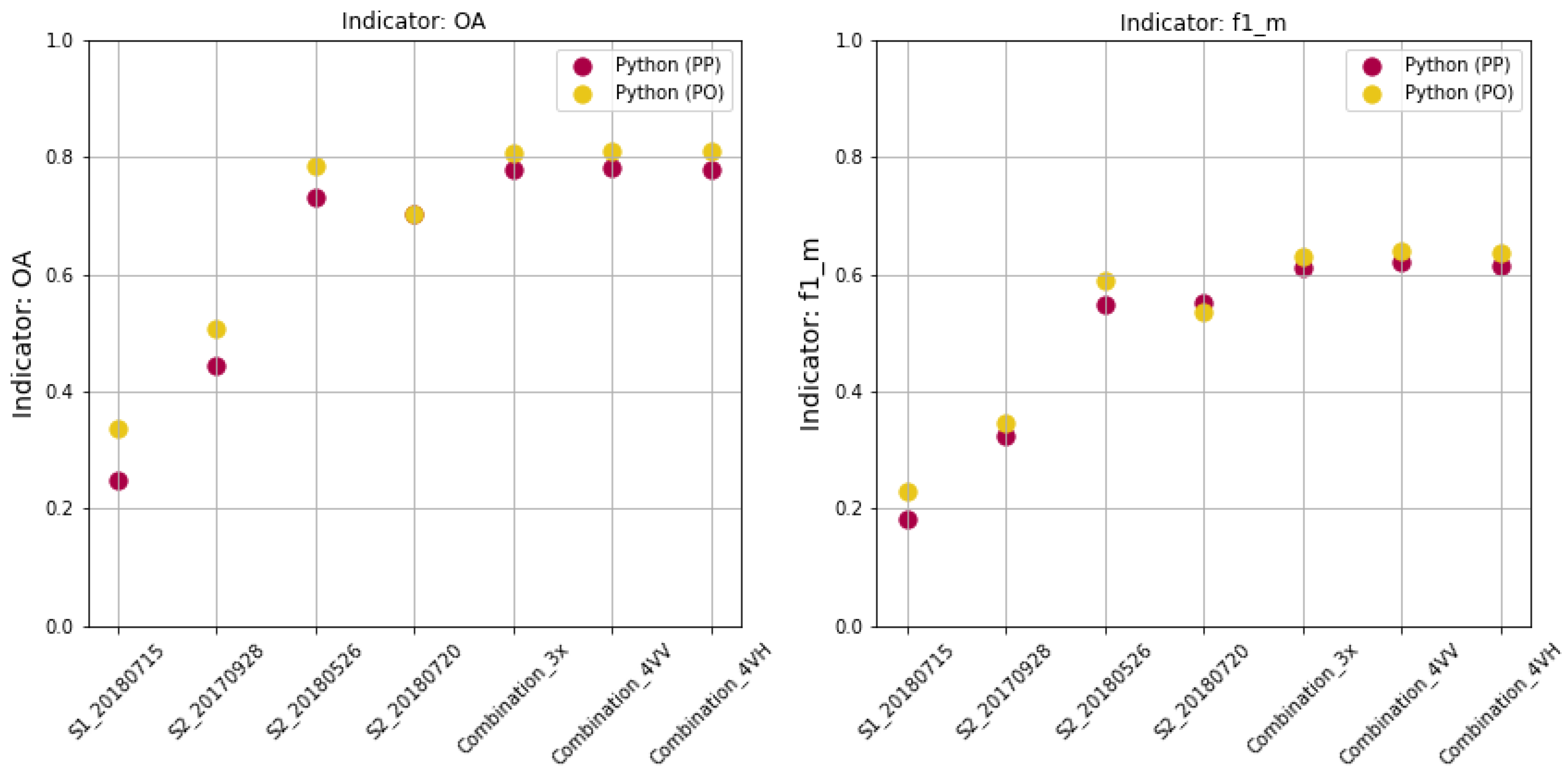
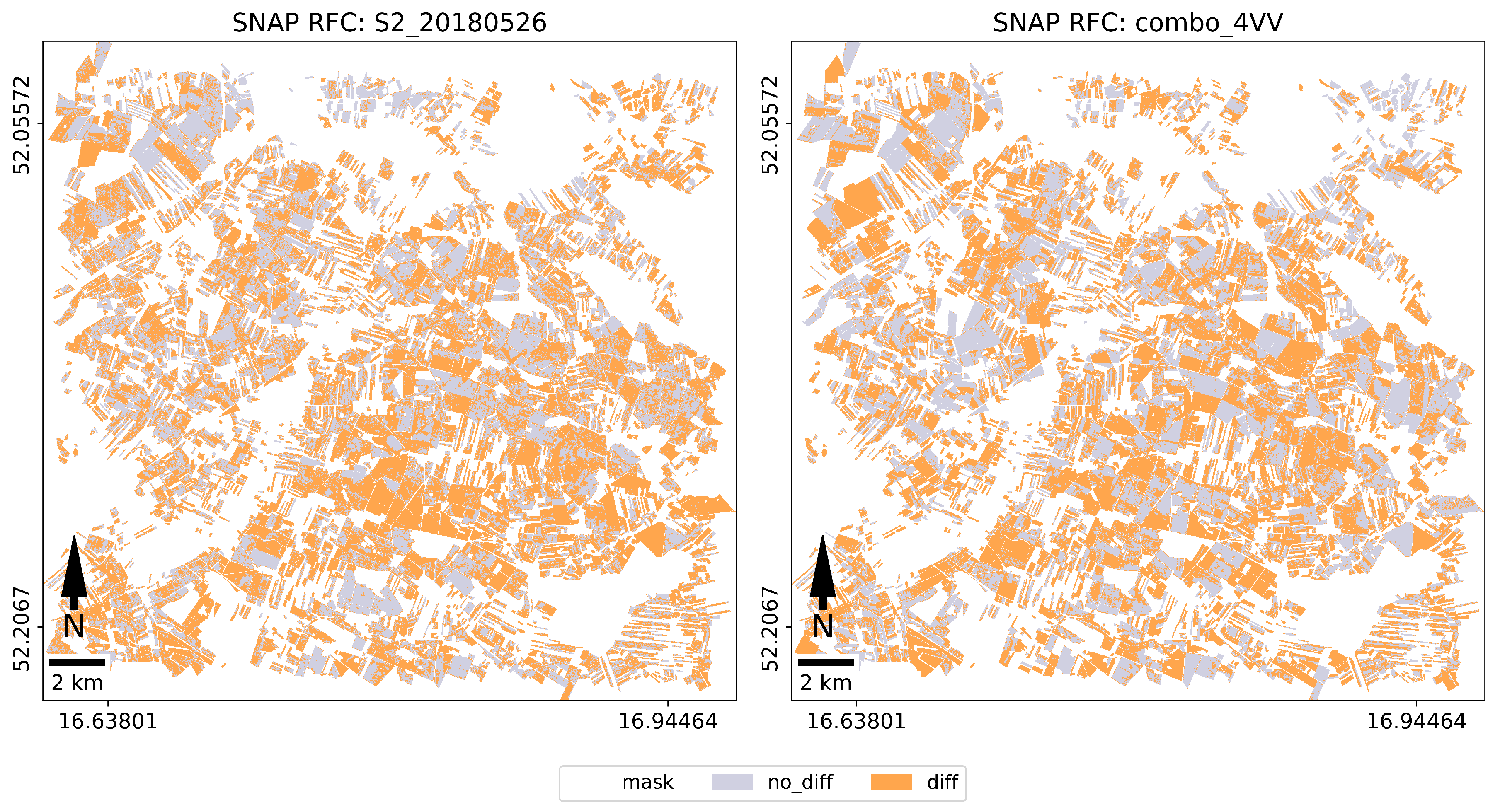
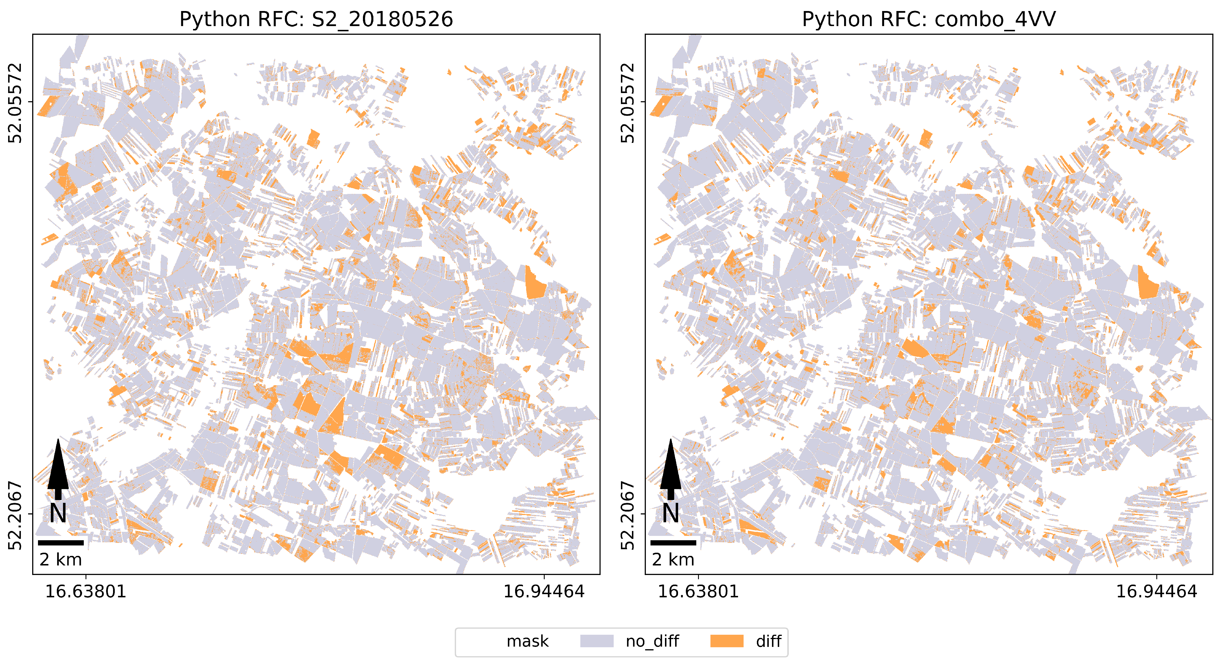
In our case, the highest accuracy (81%) was obtained in RF classification using entire training set in object-oriented approach with accuracy estimation for Combination_3x, Combination_4VV, Combination_4VH (for comparison to pixel approach - 78%). It was also astonishing that there was no large decrease in accuracy for a single image S2_20180526 (79% in Python PO and 73% in Python PP). We obtained better accuracy for one image then [16] (one Sentinel-1: 47%, one Sentinel-2: 39%), but comparable with [7,8]. The highest accuracy of 79% was for a single image registered on 26 May 2018, while the classification of the image of 20 July—just before the harvest was slightly less accurate.

The high accuracies obtained in crop recognition using time series only radar images ($OA=87\%$ [47], $OA=87\%$ [48], $OA=96.7\%$ [15]) provide valuable inspiration for future research in our test area.

5. Conclusions

Analyses of the classification accuracy of three Sentinel-2 and one Sentinel-1 images allow the following conclusions to be drawn:

1.

The accuracy metrics used in machine learning: “accuracy” and “specificity” show overestimated accuracy values because they include not only “true positive” but also “true negative” cases. This approach is valid for one class classification (e.g., medical testing) but not for the use of classification for crop recognition.

2.

Reporting the mean accuracy value as overall accuracy gives the false impression of high accuracy. In our first case (SNAP) for the image from May on the control fields, the accuracy overestimation was approx. 45% (if, instead of the correct value of 52%, we gave the average $acc\_m$ value of 94%), in the second case it was approx. 20% (instead of 79%, 97%)—compare $OA$ and $ac{c}_m$ for S2_20180526 in Table 10 and Table 12.

3.

The use of all training pixels from the reference polygons, compared to the sampling method, increases the classification accuracy with RFC algorithm by almost 40% (form 50% to 80%).

4.

The highest classification accuracy, equaling 81%, was obtained for the combination of 3 Sentinel-2 images with all pixels in our own Python script (for comparison 80% reported by [8],

5.

The overall accuracy of the single image classification was equal 79%, which is slightly higher then the value from the literature (77.4% [7], 77.2% [8]) and much better than 47% [16], the highest accuracy we obtained in May, a few weeks before harvest confirming [8],

6.

Adding radar images did not improve the classification result, which is also confirmed in the literature [20,23], but due to the use of only one Sentinel-1 image, it does not allow us to generalize this conclusion and requires further research.

The research confirmed the possibility of using a single Sentinel-2 image to screening control farmers’ declarations registered several weeks before the harvest. This conclusion is essentially due to the difficulty of acquiring cloudless multitemporal images over large areas in central Europe.

In the random forest classification method, it is recommended to use all data from the training set. It is not possible to input large training data to SNAP, but it is possible with the use of own scripts written e.g., in Python. In accuracy analyses, it is not recommended to use the metrics: accuracy and specificity, which are commonly used in machine learning, and overall accuracy should not be confused with the class mean value of accuracy. However, the following metrics seem reliable: overall accuracy, sensitivity = producer accuracy, precision = user accuracy, F1-score. The conclusion in the last paragraph, according to the authors, fills the gap in the use of the random forest algorithm in crop classification that are characterized by high variability of the spectral response within individual crops.

References

1. Devos, W.; Fasbender, D.; Lemoine, G.; Loudjani, P.; Milenov, P.; Wirnhardt, C. Discussion Document on the Introduction of Monitoring to Substitute OTSC—Supporting Non-Paper DS/CDP/2017/03 Revising R2017/809; Publications Office of the European Union: Luxembourg, 2017. [Google Scholar] [CrossRef]
2. Devos, W.; Lemoine, G.; Milenov, P.; Fasbender, D. Technical Guidance on the Decision to Go for Substitution of OTSC by Monitoring; Publications Office of the European Union: Luxembourg, 2018. [Google Scholar] [CrossRef]
3. Devos, W.; Lemoine, G.; Milenov, P.; Fasbender, D.; Loudjani, P.; Wirnhardt, C.; Sima, A.; Griffiths, P. Second Discussion Document on the Introduction of Monitoring to Substitute OTSC: Rules for Processing Application in 2018–2019; Publications Office of the European Union: Luxembourg, 2018. [Google Scholar] [CrossRef]
4. Rouse, J.; Haas, R.; Schell, J.; Deering, D.; Harlan, J. Monitoring the Vernal Advancement and Retrogradation (Green Wave Effect) of Natural Vegetation. NASA/GSFC Type III Final Report. 1974. Available online: https://ntrs.nasa.gov/api/citations/19750020419/downloads/19750020419.pdf (accessed on 14 July 2021).
5. Laur, H.; Bally, P.; Meadows, P.; Sanchez, J.; Schättler, B.; Lopinto, E.; Esteban, D. Derivation of the backscattering coefficient sigma nought in ESA ERS SAR PRI products. Technical Report ES-TN-RS-PM-HL09, ESA, September 1998. 1994. Available online: https://earth.esa.int/documents/10174/13019/ers_sar_calibration_issue2_5f.pdf (accessed on 14 July 2021).
6. Saini, R.; Ghosh, S. Crop classification on single date sentinel-2 imagery using random forest and support vector machine. Int. Arch. Photogramm. Remote Sens. Spat. Inf. Sci. 2018, 42, 683–688. [Google Scholar] [CrossRef] [Green Version]
7. Brinkhoff, J.; Vardanega, J.; Robson, A. Land cover classification of nine perennial crops using sentinel-1 and -2 data. Remote Sens. 2020, 12, 96. [Google Scholar] [CrossRef] [Green Version]
8. Maponya, M.; van Niekerk, A.; Mashimbye, Z. Pre-harvest classification of crop types using a Sentinel-2 time-series and machine learning. Comput. Electron. Agric. 2020, 169. [Google Scholar] [CrossRef]
9. Carranza-García, M.; García-Gutiérrez, J.; Riquelme, J.C. A Framework for Evaluating Land Use and Land Cover Classification Using Convolutional Neural Networks. Remote Sens. 2019, 11, 274. [Google Scholar] [CrossRef] [Green Version]
10. Kussul, N.; Lavreniuk, M.; Skakun, S.; Shelestov, A. Deep Learning Classification of Land Cover and Crop Types Using Remote Sensing Data. IEEE Geosci. Remote Sens. Lett. 2017, 14, 778–782. [Google Scholar] [CrossRef]
11. Hongyan, Z.; Jinzhong, K.; Xiong, X.; Liangpei, Z. Accessing the temporal and spectral features in crop type mapping using multi-temporal Sentinel-2 imagery: A case study of Yi’an County, Heilongjiang province, China. Comput. Electron. Agric. 2020, 176, 105618. [Google Scholar] [CrossRef]
12. Neetu; Ray, S. Exploring machine learning classification algorithms for crop classification using sentinel 2 data. Int. Arch. Photogramm. Remote Sens. Spat. Inf. Sci. 2019, 42, 573–578. [Google Scholar] [CrossRef] [Green Version]
13. Shi, Y.; Li, J.; Ma, D.; Zhang, T.; Li, Q. Method for crop classification based on multi-source remote sensing data. In Proceedings of the IOP Conference Series, Materials Science and Engineering, Kazimierz Dolny, Poland, 21–23 November 2019; Volume 592. [Google Scholar] [CrossRef] [Green Version]
14. Qadir, A.; Mondal, P. Synergistic use of radar and optical satellite data for improved monsoon cropland mapping in India. Remote Sens. 2020, 12, 522. [Google Scholar] [CrossRef] [Green Version]
15. Hütt, C.; Waldhoff, G.; Bareth, G. Fusion of sentinel-1 with official topographic and cadastral geodata for crop-type enriched LULC mapping using FOSS and open data. ISPRS Int. J. Geo-Inf. 2020, 9, 120. [Google Scholar] [CrossRef] [Green Version]
16. Van Tricht, K.; Gobin, A.; Gilliams, S.; Piccard, I. Synergistic use of radar sentinel-1 and optical sentinel-2 imagery for crop mapping: A case study for Belgium. Remote Sens. 2018, 10, 1642. [Google Scholar] [CrossRef] [Green Version]
17. Hejmanowska, B.; Mikrut, S.; Głowienka, E.; Michałowska, K.; Kramarczyk, P.; Pirowski, T. Expertise on the Use of Sentinel 1 and 2 Images to Monitor the Agricultural Activity of ARIMR Beneficiaries. 2018. Available online: http://home.agh.edu.pl/~galia/img/Raport_ARIMR_AGH_2018_EN_haslo.pdf (accessed on 14 July 2021).
18. Hejmanowska, B.; Mikrut, S.; Głowienka, E.; Kramarczyk, P.; Pirowski, T. The Use of Hyperspectral Data to Monitor the Agricultural Activity of the ARMA Beneficiaries and Support its Business Processes. 2019. Available online: http://home.agh.edu.pl/~galia/img/Raport_ARIMR_AGH_2019_EN_haslo.pdf (accessed on 14 July 2021).
19. Musiał, J.; Bojanowski, J. Assessing potential of the Sentinel-2 imagery for monitoring of agricultural fields in Poland. In Proceedings of the 25th MARS Conference, Prague, Czech Republic, 26–28 November 2019. [Google Scholar]
20. Mustak, S.; Uday, G.; Ramesh, B.; Praveen, B. Evaluation of the performance of SAR and SAR-optical fused dataset for crop discrimination. Int. Arch. Photogramm. Remote Sens. Spat. Inf. Sci. 2019, 42, 563–571. [Google Scholar] [CrossRef] [Green Version]
21. Phalke, A.R.; Özdoğan, M.; Thenkabail, P.S.; Erickson, T.; Gorelick, N.; Yadav, K.; Congalton, R.G. ISPRS Journal of Photogrammetry and Remote Sensing Mapping croplands of Europe, Middle East, Russia, and Central Asia using Landsat, Random Forest, and Google Earth Engine. ISPRS J. Photogramm. Remote Sens. 2020, 167, 104–122. [Google Scholar] [CrossRef]
22. Sun, C.; Bian, Y.; Zhou, T.; Pan, J. Using of multi-source and multi-temporal remote sensing data improves crop-type mapping in the subtropical agriculture region. Sensors 2019, 19, 2401. [Google Scholar] [CrossRef] [PubMed] [Green Version]
23. Sun, L.; Chen, J.; Guo, S.; Deng, X.; Han, Y. Integration of time series sentinel-1 and sentinel-2 imagery for crop type mapping over oasis agricultural areas. Remote Sens. 2020, 12, 158. [Google Scholar] [CrossRef] [Green Version]
24. Hu, X.; Yang, W.; Wen, H.; Liu, Y.; Peng, Y. A Lightweight 1-D Convolution Augmented Transformer with Metric Learning for Hyperspectral Image Classification. Sensors 2021, 21, 1751. [Google Scholar] [CrossRef]
25. Stehman, S.V.; Foody, G.M. Key issues in rigorous accuracy assessment of land cover products. Remote Sens. Environ. 2019, 231, 111199. [Google Scholar] [CrossRef]
26. Morales-Barquero, L.; Lyons, M.B.; Phinn, S.R.; Roelfsema, C.M. Trends in Remote Sensing Accuracy Assessment Approaches in the Context of Natural Resources. Remote Sens. 2019, 11, 2305. [Google Scholar] [CrossRef] [Green Version]
27. Hord, M.R.; Brooner, W. Land-Use Map Accuracy Criteria. Photogramm. Eng. Remote Sens. 1976, 42, 671–677. [Google Scholar]
28. Van Genderen, J.; Lock, B. Testing Land Use Map Accuracy. Photogramm. Eng. Remote Sens. 1977, 43, 1135–1137. [Google Scholar]
29. Gineva, M.E. Testing Land-Use Map Accuracy: Another Look. Photogramm. Eng. Remote Sens. 1979, 45, 1371–1377. [Google Scholar]
30. Russell, G.C. A review of assessing the accuracy of classifications of remotely sensed data. Remote Sens. Environ. 1991, 37, 35–46. [Google Scholar] [CrossRef]
31. Canran, L.; Paul, F.; Lalit, K. Comparative assessment of the measures of thematic classification accuracy. Remote Sens. Environ. 2007, 107, 606–616. [Google Scholar] [CrossRef]
32. Pontus, O.; Foody, G.M.; Stehman, S.V.; Woodcock, C.E. Making better use of accuracy data in land change studies: Estimating accuracy and area and quantifying uncertainty using stratified estimation. Remote Sens. Environ. 2013, 129, 122–131. [Google Scholar] [CrossRef]
33. Foody, G.M. Impacts of Sample Design for Validation Data on the Accuracy of Feedforward Neural Network Classification. Appl. Sci. 2017, 7, 888. [Google Scholar] [CrossRef] [Green Version]
34. Luo, D.; Goodin, D.G.; Caldas, M.M. Spatial–Temporal Analysis of Land Cover Change at the Bento Rodrigues Dam Disaster Area Using Machine Learning Techniques. Remote Sens. 2019, 11, 2548. [Google Scholar] [CrossRef] [Green Version]
35. Gbodjo, Y.J.E.; Ienco, D.; Leroux, L.; Interdonato, R.; Gaetano, R.; Ndao, B. Object-Based Multi-Temporal and Multi-Source Land Cover Mapping Leveraging Hierarchical Class Relationships. Remote Sens. 2020, 12, 2814. [Google Scholar] [CrossRef]
36. Tao, L.; Lexie, Y.; Dalton, L. Change detection using deep learning approach with object-based image analysis. Remote Sens. Environ. 2021, 256, 112308. [Google Scholar] [CrossRef]
37. Foody, G.M. Impacts of ignorance on the accuracy of image classification and thematic mapping. Remote Sens. Environ. 2021, 259, 112367. [Google Scholar] [CrossRef]
38. Fawcett, T. An introduction to ROC analysis. Pattern Recognit. Lett. 2006, 27, 861–874. [Google Scholar] [CrossRef]
39. Shetty, S.; Gupta, P.K.; Belgiu, M.; Srivastav, S.K. Assessing the Effect of Training Sampling Design on the Performance of Machine Learning Classifiers for Land Cover Mapping Using Multi-Temporal Remote Sensing Data and Google Earth Engine. Remote Sens. 2021, 13, 1433. [Google Scholar] [CrossRef]
40. Csillik, O.; Belgiu, M.; Asner, G.P.; Kelly, M. Object-Based Time-Constrained Dynamic Time Warping Classification of Crops Using Sentinel-2. Remote Sens. 2019, 11, 1257. [Google Scholar] [CrossRef] [Green Version]
41. Mercier, A.; Betbeder, J.; Baudry, J.; Le Roux, V.; Spicher, F.; Lacoux, J.; Roger, D.; Hubert-Moy, L. Evaluation of Sentinel-1 and 2 time series for predicting wheat and rapeseed phenological stages. ISPRS J. Photogramm. Remote Sens. 2020, 163, 231–256. [Google Scholar] [CrossRef]
42. Demarez, V.; Helen, F.; Marais-Sicre, C.; Baup, F. In-season mapping of irrigated crops using Landsat 8 and Sentinel-1 time series. Remote Sens. 2019, 11, 118. [Google Scholar] [CrossRef] [Green Version]
43. Liu, X.; Zhai, H.; Shen, Y.; Lou, B.; Jiang, C.; Li, T.; Hussain, S.; Shen, G. Large-Scale Crop Mapping from Multisource Remote Sensing Images in Google Earth Engine. IEEE J. Sel. Top. Appl. Earth Obs. Remote Sens. 2020, 13, 414–427. [Google Scholar] [CrossRef]
44. Nanshan, Y.; Jinwei, D. Examining earliest identifiable timing of crops using all available Sentinel 1/2 imagery and Google Earth Engine. ISPRS J. Photogramm. Remote Sens. 2020, 161, 109–123. [Google Scholar] [CrossRef]
45. Mohite, J.D.; Sawant, S.A.; Rana, S.; Pappula, S. Wheat area mapping and phenology detection using synthetic aperture radar and multi-spectral remote sensing observations. Int. Arch. Photogramm. Remote Sens. Spat. Inf. Sci. 2019, XLII-3/W6, 123–127. [Google Scholar] [CrossRef] [Green Version]
46. Feng, S.; Zhao, J.; Liu, T.; Zhang, H.; Zhang, Z.; Guo, X. Crop Type Identification and Mapping Using Machine Learning Algorithms and Sentinel-2 Time Series Data. IEEE J. Sel. Top. Appl. Earth Obs. Remote Sens. 2019, 12, 3295–3306. [Google Scholar] [CrossRef]
47. Xie, Q.; Lai, K.; Wang, J.; Lopez-Sanchez, J.M.; Shang, J.; Liao, C.; Zhu, J.; Fu, H.; Peng, X. Crop Monitoring and Classification Using Polarimetric RADARSAT-2 Time-Series Data Across Growing Season: A Case Study in Southwestern Ontario, Canada. Remote Sens. 2021, 13, 1394. [Google Scholar] [CrossRef]
48. Valcarce-Diñeiro, R.; Arias-Pérez, B.; Lopez-Sanchez, J.M.; Sánchez, N. Multi-Temporal Dual- and Quad-Polarimetric Synthetic Aperture Radar Data for Crop-Type Mapping. Remote Sens. 2019, 11, 1518. [Google Scholar] [CrossRef] [Green Version]
Figure 1. The scheme of the methodology.
Remotesensing 13 03176 g001
Figure 2. Test area location (UL: 16°37′21.43″E; 52°14′31.3″N; LR: 16°57′48.28″E; 52°1′3.74″N). Data source: OpenStreetMap.
Remotesensing 13 03176 g002
Figure 3. Declared agricultural parcels.
Remotesensing 13 03176 g003
Figure 4. The impact of the image registration date and the number of classified images on the classification accuracy-selected metrics: OA and f 1 m . Classification in SNAP with RF algorithm with sampling method (50,000 training/50,000 validation samples). Accuracy assessment on validation set—red points, on test set: pixel approach—yellow points, object approach—purple points.
Remotesensing 13 03176 g004
Figure 5. The impact of the image registration date and the number of classified images on the accuracy of classification-selected indicators: O A and f 1 m . Classification is performed in our own Python scripts with RFC algorithm. Accuracy assessment in our own scripts: Python (PP) and Python (PO).
Remotesensing 13 03176 g005
Figure 6. Accuracy metrics calculated for the result of the classification performed in SNAP using 50000 and 5000 training samples. For comparison, the O A obtained in the classification using our own scripts in Python (black dashed line).
Remotesensing 13 03176 g006
Figure 7. Map of discrepancies between farmers’ declarations and classification results (UTM34N coordinate). RF classification—sampling 50,000 pixels. Confirmation in gray, difference between declared and classified crop—brown.
Remotesensing 13 03176 g007
Figure 8. Map of discrepancies between farmers’ declarations and classification results (UTM34N coordinate). RF classification—the entire training set: 1,412,092 pixels. Confirmation in gray, difference between declared and classified crop—brown.
Remotesensing 13 03176 g008