Abstract
This study aims to assess the feasibility of delineating and identifying mineral ores from hyperspectral images of tin–tungsten mine excavation faces using machine learning classification. We compiled a set of hand samples of minerals of interest from a tin–tungsten mine and analyzed two types of hyperspectral images: (1) images acquired with a laboratory set-up under close-to-optimal conditions, and (2) a scan of a simulated mine face using a field set-up, under conditions closer to those in the gallery. We have analyzed the following minerals: cassiterite (tin ore), wolframite (tungsten ore), chalcopyrite, malachite, muscovite, and quartz. Classification (Linear Discriminant Analysis, Singular Vector Machines and Random Forest) of laboratory spectra had a very high overall accuracy rate (98%), slightly lower if the 450–950 nm and 950–1650 nm ranges are considered independently, and much lower (74.5%) for simulated conventional RGB imagery. Classification accuracy for the simulation was lower than in the laboratory but still high (85%), likely a consequence of the lower spatial resolution. All three classification methods performed similarly in this case, with Random Forest producing results of slightly higher accuracy. The user’s accuracy for wolframite was 85%, but cassiterite was often confused with wolframite (user’s accuracy: 70%). A lumped ore category achieved 94.9% user’s accuracy. Our study confirms the suitability of hyperspectral imaging to record the spatial distribution of ore mineralization in progressing tungsten–tin mine faces.
1. Introduction
Hyperspectral images produced by imaging spectrometers are 3D arrays in which each voxel holds a radiance spectrum that is processed to reflectance [1,2]. The acquisition of single reflectance spectra with spectrometers in the visible, near-infrared, and short-wave infrared wavelength domains (400–2500 nm) is a relatively simple and non-invasive technique that has been used in the laboratory and the field for decades ago [3,4]. The particular optical and electronic properties of each material result, under illumination results in specific spectral features that are often diagnostic of given minerals and rocks [5,6,7], although the influence of variations in illumination and viewing geometry, the macro-structure of the sample, and the presence of mixtures in the field-of-view, tend to reduce the diagnostic power of reflectance spectra. Extending point readings to a hyperspectral image has two main advantages. First, the 2D result allows considering the spatial distribution of different materials in the imaged scene. Second, in case of a crude identification, being able to delimit a given uncertain material facilitates an accurate sampling for complementary techniques such as X-ray diffraction (XRD) or X-ray fluorescence (XRF).
Most hyperspectral images have been remotely acquired from airborne sensors and a few satellites and, in the context of the mining industry, common applications of remotely-sensed hyperspectral images are mineral exploration (see examples in [8,9,10,11,12]) and the environmental impact [13,14,15]. Currently, close-range hyperspectral images of hand samples and/or drill cores [16,17,18,19], along with ground-based panoramic hyperspectral imaging of semi-vertical outcrops [20,21,22,23,24], are increasingly used as hyperspectral imaging systems become more portable and widespread. Multi- and hyperspectral image systems have also been developed for ore microscopy [25,26,27,28] with the aim of achieving a quantitative mineralogical analysis. In their extensive review, Krupnik and Khan [24] organize very recent articles (most of them published after 2010) reporting close-range hyperspectral imaging applications, which mainly deal with the analysis of economically valued materials (32 studies, of which 13 focus on the validation of spectral identification methods), and environmental impact (13 studies). Horizontal and oblique ground-based hyperspectral imaging of vertical structures (cliffs, road cuts, open-pit walls…) can be integrated with digital topography, which can be retrieved from either terrestrial LiDAR data [29] or Structure from Motion (SfM) processing of conventional photographs [30,31].
An extended panoply of methods has been developed for the analysis of remotely sensed hyperspectral images, (e.g., [32,33,34]), which are also being applied to close-range hyperspectral images, and few multi-scale studies have been undergone [17,35] (Amigo [2] compiles a number of modern methods that can be applied to both remote and close-range hyperspectral imagery. Machine learning methods, in particular supervised classification methods, have become common for the analysis of hyperspectral images [36,37,38]), and are starting to be applied to close-range imagery for the automatic identification and mapping of different materials within the imaged sample. Murphy et al. [20] acquired both point spectra and ground-based hyperspectral images of vertical faces in an iron-ore mine from a distance of 30 m in the visible and near-infrared (VISNIR) and short-wave infrared (SWIR). The authors compared spectral angle mapping (SAM) and support vector machines (SVM) to classify materials such as shale, manganiferous-shale, goethite, martite, and chert, taking shadowing effects into account. While SVM outperformed SAM under uniform illumination conditions, SAM was more robust to the presence of shadows unless shadowed training spectra were provided to the SVM classifier. Additionally, SAM performed better than SVM if training spectra were selected from a spectral library, instead of from within the image itself. Krupnik and Khan [24] also presented their own case studies of close-range hyperspectral panoramic imaging for the characterization of semi-vertical outcrops (faults, pits, roadcuts and quarry settings). They applied SVM and the Multi-range Spectral Feature Fitting (SFF) to produce classified images of materials such as limestone, siltstone, shale, hematitic siltstone, calcite, illite, jarosite, iron oxides, and dolomite. They also obtained considerable geological information from mapping the wavelength and depth of absorption features in selected wavelength ranges, which they applied as well later [39] to analyze hyperspectral images of small, laboratory-prepared mixtures of limestone minerals (calcite, dolomite, and chert), with results that were consistent to those provided by point count. The same study reports a successful mapping of mixtures in hyperspectral images of small rock chips by applying machine learning methods and using the spectra of known mixtures as references. López-Benito et al. [28] applied classification methods for the analysis of microscope hyperspectral images in the VISNIR (350–1000 nm) range for the automated identification of metallic ore species, which was achieved with a very high accuracy.
Building and updating 3D models to quantitatively characterize the distribution and heterogeneity of ore grade, vein thickness, orientation, and network geometry are critical for the mining industry as it provides a better understanding of the mineralization with important benefits for the management and optimization of the exploitation; thus, reducing the environmental impact. Typically, these 3D models are based on knowledge of the site’s structural geology, with geophysical exploration contributing to provide a better understanding of the deposit. Image data acquired from the mine excavation itself could be used to confirm or update these models, monitoring the ore grade and distribution. In this regard, we aim at integrating proximal ground-based conventional and hyperspectral imaging of the mine excavation face to provide the ore grade and 2D geometry of the mineralization in the section. Ideally, a 3D tomography could be derived from these 2D planes as the excavation front progresses.
Deployment and operation of hyperspectral imaging systems in the field is always involved and doing so under gallery mine conditions is challenging. As a previous step to actually acquire, process and analyze hyperspectral images of a mine excavation face, here we explore the feasibility and interest of such an approach by using hand samples that feature the minerals of interest. For this purpose, we conducted the following studies:
- Laboratory imaging spectrometry. We scanned the hand samples using hyperspectral cameras on a laboratory set-up to assess spectral separability and evaluate machine learning classification methods under close-to-optimal conditions.
- Simulation of hyperspectral imaging of the mine face. We scanned the whole set of hand samples with the same field set-up, illumination, and distance to object that are expected to be used in the mine gallery, evaluating machine learning methods to identify and map the distribution of materials in the resulting image.
2. Geological Settings
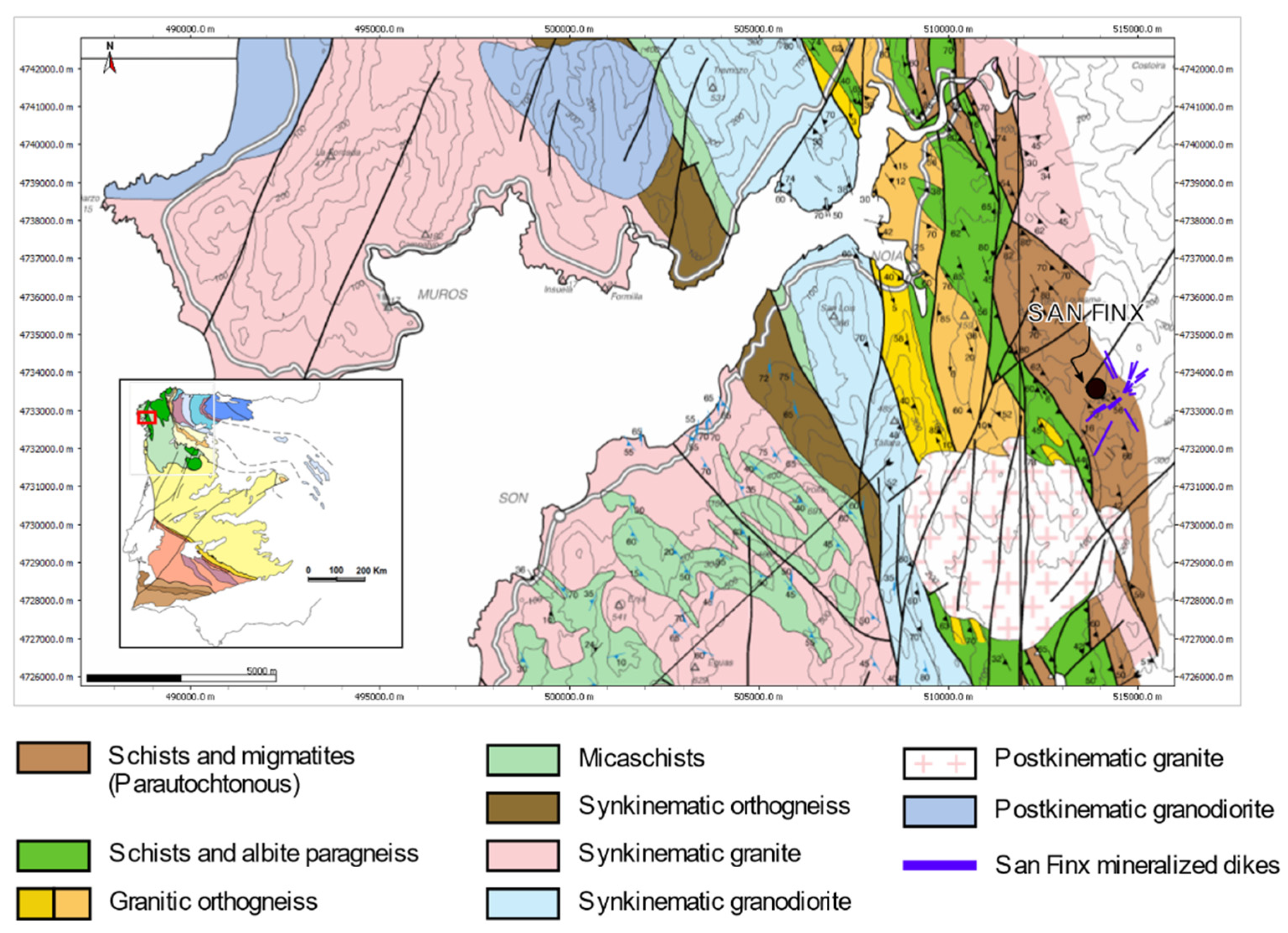
The studied samples were collected in the San Finx tin–tungsten mine, which is located in Lousame, A Coruña, Galicia, NW Spain (Figure 1). San Finx is a typical case of Late Palaeozoic, granite-related hydrothermal deposit, associated with the European metallogenic belt. Tin–tungsten ore is directly related to granites formed from Late Devonian to Permian during the Variscan or the so-called Hercynian orogeny, resulting from the continental collision of Laurussia and Gondwana [40]. The San Finx mineralization consists of a subvertical set of quartz lodes prevalent in the N 50° E direction, which at its eastern end shows pegmatitic features (e.g., the occurrence of K-feldspar). This lode field reaches more than 1 km in length, and the lode thickness varies between 0.5 and 1.5 m [41]. Host rocks consist of schists, migmatites and granites, while the metallogenesis consists of Sn–W–Ta–Nb–Mo–Cu–As–Au–A–Bi. The exploited ore minerals are cassiterite and wolframite. Other minerals occurring in the quartz lodes are arsenopyrite, pyrite, scheelite, chalcopyrite, molybdenite columbite-tantalite, muscovite, and tourmaline, among others [42,43].
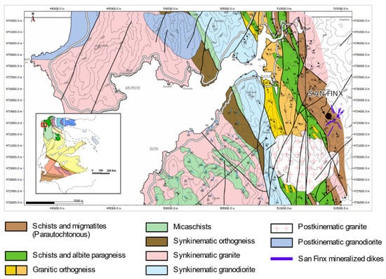
Figure 1.
Geological context and situation of the San Finx mine [44].
3. Materials and Methods
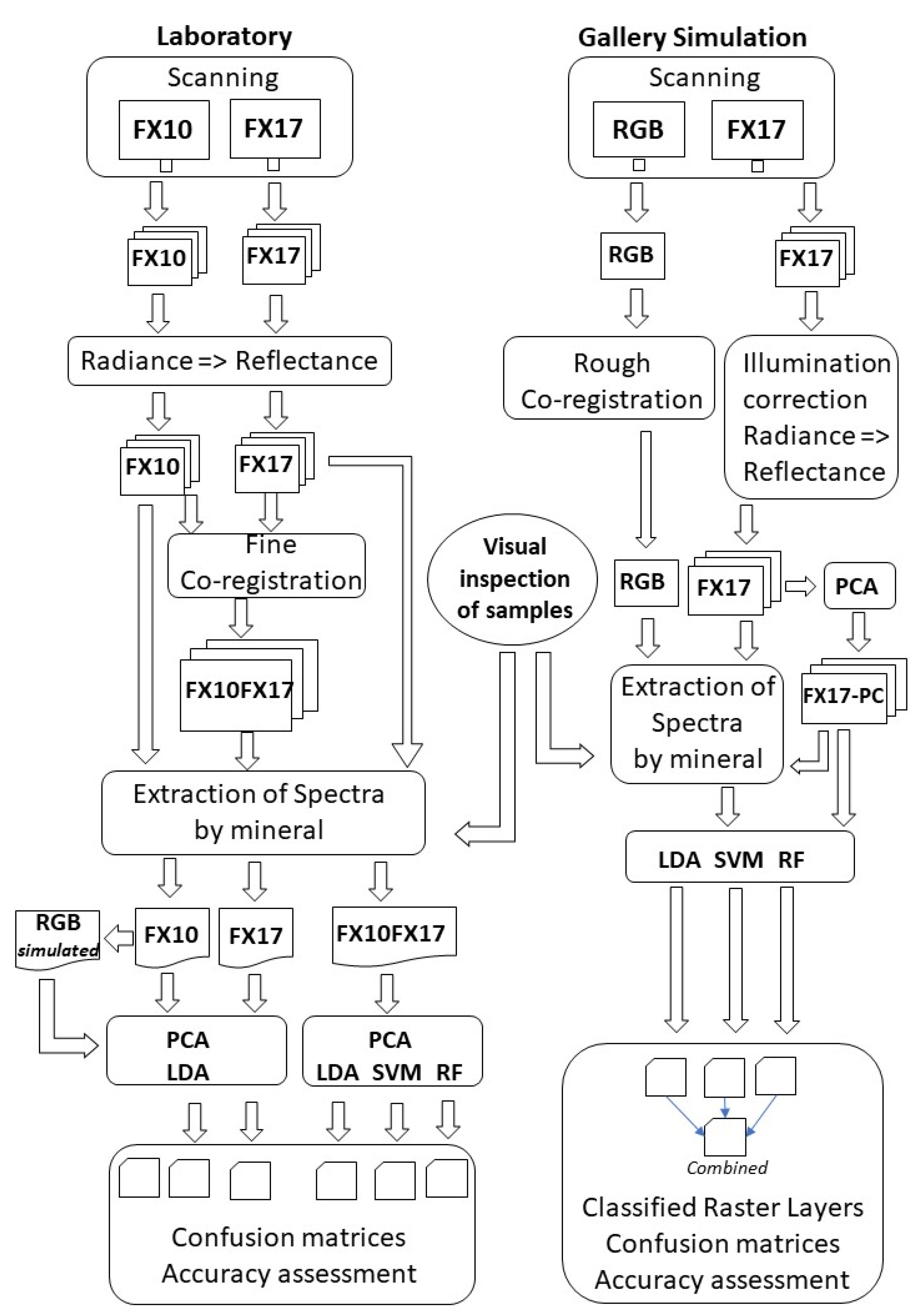
See methods flowchart (Figure 2).
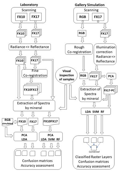
Figure 2.
Workflow of the methodology.
3.1. Laboratory Imaging Spectrometry
In order to achieve close-to-optimal conditions, we scanned samples from the mine with Specim FX10 and FX17 cameras (Table 1) consecutively mounted on the same Specim LabScanner Setup 40 × 20 and with care not to move the samples between each scan. We used Specim’s Lumo software for scanning, which renders hyperspectral images of radiance for the whole scanned area, and two images of, respectively, the dark (internal shutter) and white references, which we used to calculate images of spectral reflectance for each camera.

Table 1.
Specifications of images acquired with Specim cameras FX10 and FX17. FWHM: full width height maximum; FOV: field of view; SNR: signal to noise ratio.
We co-registered the FX17 reflectance images to their FX10 counterparts based on bands corresponding to the common part of the wavelength range and stacked the resulting FX10 and FX17 co-registered reflectance images into one single reflectance image of 628 bands for each sample and spatial resolution of 0.224 mm/pixel. In order to perform reflectance calculation, co-registration, band stacking, and cropping, we developed in-house software consisting of R [45] scripts (packages raster [46], rgdal [47], RStoolbox [48], gdalUtilities [49] and link2GI [50], which call commands of GDAL [51], OTB [52] and pktools [53]). The co-registration processing proceeded in two steps. First, we ran a first-order polynomial warp with homologous points automatically extracted by the SIFT method (HomologousPointExtraction in OTB [54]). Second, the co-registration was refined by calculating subtle local X and Y shifts that optimized local correlation between the corresponding bands of both cameras (FineRegistration in OTB). Geometric transformations were calculated using corresponding bands of the same wavelength in both cameras and then applied to all bands of FX17 (GridBasedImageResampling in OTB). We discarded some bands at the extremes of each camera because of noisy appearance, and left the hyperspectral data to be in the 450–950 nm (FX10) and 950–1650 nm (FX17) ranges.
Hyperspectral images were displayed and sets of pixel spectra (a total of 110) were interactively extracted for each mineral with the EnMAP Box plugin [55] of QGIS [56], which required combining photo-interpretation and direct visual inspection of the samples. Different color composites, including those combining different PCs, were used to emphasize limits among materials and facilitate pixel selection. Finally, we imported the spectra into R, where we created comparative graphics along with reference spectra extracted from spectral libraries by USGS [57] and JPL [58,59] and ran statistical analysis. We calculated matrices of dissimilarities using the Jeffries–Matusita metric [60] to measure the spectral resolving power of each camera (FX10, FX17, and combined FX10_FX17). We also simulated the RGB values of a conventional camera (Canon 60D) from the FX10 values using camera spectral sensitivity curves [61] and calculated the RGB dissimilarity matrix with these values as well to evaluate the power of conventional photos to identify the minerals of interest. Finally, we ran three different classification methods: Linear Discriminant Analysis (LDA), Singular Vector Machines (SVM), and Random Forest (RF) for each of the four datasets (FX10, FX17, combined FX10_FX17, and Canon 60D), whose basics are briefly introduced in Section 3.3. To this end, we used R packages MASS [62], e1071 [63], randomForest [64], and caret [65].
3.2. Ground-Based Panoramic Hyperspectral Imaging of Simulated Mine Face
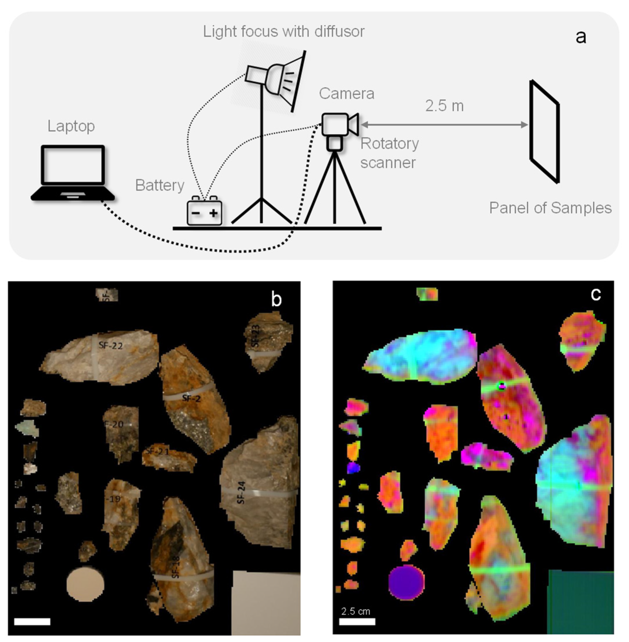
In order to prepare for the deployment of the hyperspectral equipment and analyze hyperspectral imagery acquired under conditions closer to those in the mine, we assembled a panel of 52 cm × 57 cm with the samples, along with a white reference (Sphere Optics SG 3141 95%), a Multi-Component Wavelength Standard reference (Labsphere WCS-MC-020) and a color chart (Figure 3). The image was acquired in a dark room by a Specim FX17 camera mounted on a Specim Rotary scanner on top of a tripod at a distance of 2.5 m from the lens to the panel. This distance was selected as a realistic choice in the gallery. Illumination was provided by a Fresnel Filmgear 650 w 3200 k studio light with a diffuser behind and above the camera. All systems were powered by batteries as they would be under gallery mine conditions. Image resolution was 2.6 mm/pixel and covered an area of 166.4 cm (height) × 106.1 cm (width), from which the subscene corresponding to the samples in the panel was extracted. In brief, we used, under indoor conditions, the same equipment, geometry, and illumination as would be used in the real mine gallery, for which our imagery is a close simulation of that acquired in the mine itself.

Figure 3.
(a) Field set-up for the simulation of gallery conditions. (b) Conventional digital RGB photograph of the panel of samples. (c) Color composite of the first three principal components of the hyperspectral image.
Despite the diffuser, some illumination unevenness could be appreciated, which we solved by applying a Rolling Ball Background Subtraction [66] in Fiji [67] to the first Principal Component (PC-1) and then by applying the inverse transformation. As in the case of laboratory images, the resulting hyperspectral image was displayed in QGIS making use of different color composites, which included combinations of PCs. Sets of pixel spectra (a total of 2450) for each mineral and other targets (Supplementary, Table S1) were extracted by interactively digitizing training and validation polygons, a task that required direct visual inspection of the samples as well. Finally, we input the file of polygons along with the PC-transformed hyperspectral image to the classifiers (LDA, SVM, and RF) and their respective accuracy assessments. In this case, we kept 12 components (accounting for 99.85% of the total variance) as higher components appeared too noisy. Each classifier produced a predicted map of the panel materials according to the pre-defined set of categories (Supplementary, Table S1). We used tools in EnMAP Box [34], which are based on scikit-learning, for SVM and RF classification, while R packages MASS [62] and raster [46] were used for PCA and LDA as in the case of the laboratory spectra. As combining results of different methods produces more robust results, we also combined the classifications by selecting, for each pixel, the class that had been predicted by most methods. For those pixels, in which each method was predicting a different class, we selected the class predicted by the classifier with the highest accuracy.
3.3. Classification Processing
3.3.1. Linear Discriminant Analysis (LDA)
Linear Discriminant Analysis, such as Principal Component Analysis (PCA), is often used as a dimensionality reduction technique before machine learning applications. LDA seeks to project the dataset in a space of fewer dimensions with maximum separability among classes, by maximizing the relationship between the within-class variance and the among classes variance. Unlike PCA, which is an unsupervised algorithm (it does not require training polygons for each class as it maximizes total variance for each principal component), LDA is supervised: it transforms the original space into components that linearly maximize the separation among classes, based on estimates of the mean and covariance matrix of each class, which are calculated on a training set of labelled observations [60,68]. Classification is performed by applying a Bayes rule assuming multi-variate Gaussian distributions of common variance, which simplifies to the nearest centroid rule modulo the prior class probabilities in the transformed space, as the covariance matrix becomes the identity matrix. For the present work, we performed LDA using R with package MASS [62] for both the laboratory spectra and the hyperspectral image of the panel.
3.3.2. Support Vector Machines (SVM)
As comprehensively explained in [68], SVM are a generalization of the Maximal Margin Classifier (MMC). Given a p-dimensional space of descriptors and a simple binary (2 classes) problem with n training observations (the method can be generalized to >2 classes), the MMC seeks an n-1 hyperplane that linearly separates the two classes with the maximum margin (that is: with the maximum distance from the nearest point of each class to the hyperplane). Maximizing the margin increases the chances of having a correct classification of the rest of the observations (those not included in the training set). On some occasions, the distribution of the observations is such that the correct separation of the 2 classes according to MMC implies that the maximal margin hyperplane still lies very close to some observations and the distance between margins is very narrow. In these cases, a more tolerant approach defining a wider margin even at the expense of some errors in the classification of the training set would result in fewer errors with newer observations. This method is named Support Vectors Classification (SVC) by [68] and linearSVC in the scikit-learn library [69]. The degree of tolerance is based on the relative distances from observations to their class margin: observations at the correct side of their margin or on the margin itself are at a distance 0; observations beyond the margin of their respective class but within the limit of the hyperplane are at distances 0 < e < 1, while those at the wrong side of the hyperplane are at distances > 1. The user sets the total tolerance (named “regularization” in the SVM jargon), that is, the allowed sum of all distances from observations to margins. For C = 0 there is no tolerance, so hyperplane and margins are set according to MMC. At increasing values of C, the margins can be progressively widened, with progressively more observations being left at the wrong side of the margin or even at the wrong side of the hyperplane and, actually, the hyperplane itself changes as different observations are included. Parameter C, thus, controls the number of observations that are actually involved in computing the hyperplane and its margins. It is important to note that unlike other classification approaches such as LDA, SVM classification depends only on those observations lying on the margins or beyond them, and these observations are known as support vectors (as each observation is a vector of p descriptors). An optimal value for C is calculated by k-fold cross-validation in the training set for a predefined range of C values.
There are cases in which no hyperplane can separate the classes, no matter the value of C. In these cases, rather than fitting non-linear functions, the SVM approach is to increase the dimensionality by adding new dimensions that are non-linear transforms of the p original ones. As the parameters defining the hyperplane in SVC (or linear SVC) are found based on the inner product between all pairs of training observations, SVM classification (named SVC in scikit-learn) uses a kernel-based approach for this purpose. Popular kernels in SVM classification are the polynomial and, in particular, the radial basis function (RBF), which was used in this study because of its flexibility. For RBF, we had, for any two training observations x, y (vectors in space of p descriptors):
where γ is a positive constant that can be thought of as the inverse of the variance: for low values of γ the class will be very wide, and for small values the class will be narrow. As for the case of C, γ can be set by cross-validation within a grid-search strategy as is the case of EnMAP Box. R package caret, instead, uses an analytical formula to obtain reasonable estimates of γ and fix it to that value [65].
z = exp(γ|| x − y ||2)
3.3.3. Random Forest
Random forest classification [70] is a development of classification trees. Classification trees are produced by binary and hierarchically splitting the training set by thresholding the descriptors [68]. At each level, all descriptors are sequentially tried and the best threshold for the best predictor is selected to optimize a class purity metric such as the Gini index. Once the tree is grown in the top-down direction, it is then simplified (“pruned” in the classification trees jargon) in the bottom-up direction according to an error minimization rule. One problem with classification trees is that while the fit to the training set can be very good, the prediction of new cases is very dependent upon the specific training set that was used.
Results are greatly improved by Random Forests, which introduce two modifications: a set of n trees is constructed (with no pruning) instead of just one, and only a subset of m descriptors is used. The training set is resampled with replacement in n bootstrapped sets and a classification tree is produced for each set, but only a random selection of m descriptors is considered at each level. Each tree is then applied to the test data, which yields as many predictions as bootstrapped training sets, and the final result is the set of most commonly selected (“voted”) class. A value of m = sqrt(p) is a common recommendation, and the number of trees (n) should be large enough to ensure that all descriptors were considered. In our case, we used 500 trees with the laboratory FX10FX17 dataset, while a search between 300 and 1000 selected 350 as the best number of trees for the FX17 image of the panel.
3.3.4. Validation
Validation was conducted through the analysis of confusion matrices, which were built by cross-validation: leave-one-out in the case of LDA and 10-fold cross validation in the case of SVM and RF. We calculated standard metrics from the confusion matrices using R package caret: overall accuracy (OA), user’s accuracy (UA), producer’s accuracy (PA), and F1 (which is the harmonic mean of user’s and producer’s accuracy [71,72,73]. Specifically, considering pixels in the digitized polygons,
4. Results
4.1. Laboratory Imaging Spectrometry
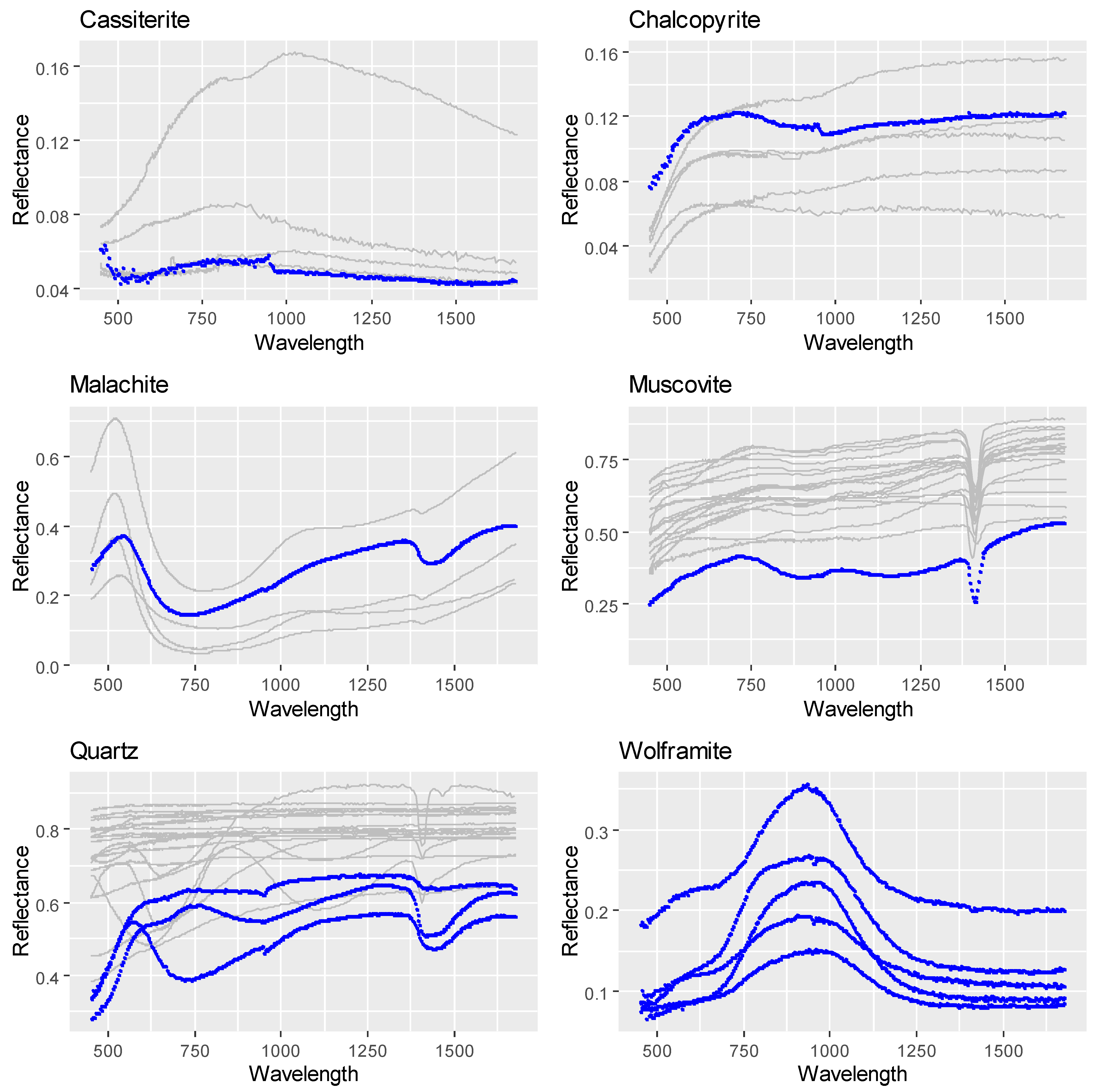
Reflectance spectra of single-mineral polygons of cassiterite, malachite, and muscovite measured in this work were similar to those found in the reference spectral libraries (Figure 4). Those of quartz targets were highly variable (as in the case of spectral libraries) because these spectra were very dependent upon the presence of other minerals or fluid inclusions as well as the effect on the optical properties of quartz of impurities and crystalline disorder. In the case of chalcopyrite, a set of spectra was much brighter than the rest of the studied minerals, and also than those from the spectral libraries. This was probably because of specular reflection from well-developed crystals. No reference spectra of wolframite could be found in the spectral libraries. In some cases, the spectra unveiled errors in the “de visu” identification of minerals in the hand samples. These spectra were discarded after the re-examination of the samples confirmed the erroneous original labelling.
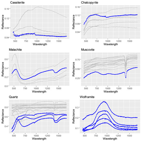
Figure 4.
Spectra retrieved from hyperspectral images acquired by scanning samples with Specim cameras FX10 and FX17 in the laboratory (blue). Reference spectra from spectral libraries USGS [57] and JPL [58,59] represented in light gray whenever available.
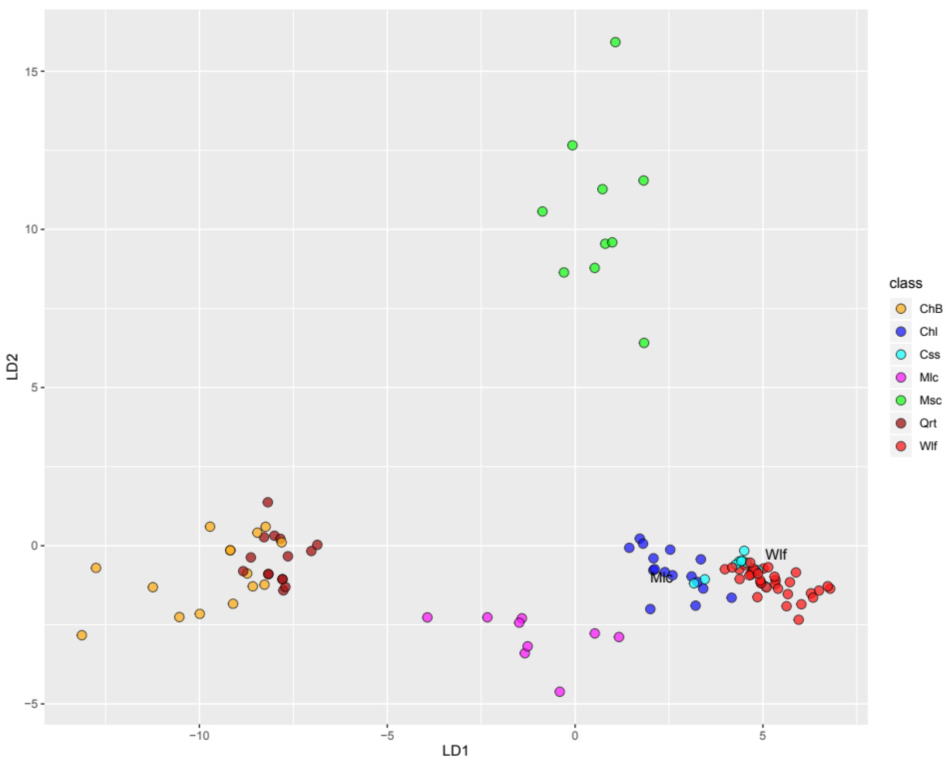
Spectral separability (Jeffries–Matusita index) among combined spectra of both cameras (450–1650 nm) was very high (>1.99) for all mineral pairs. In accordance, the LDA classification had a very high accuracy (98%, Table 2), a maximum that was achieved with 15 components. Spectral differences were well mapped in the LDA space (Figure 5), in which spectral samples were well ordinated in consistency with their respective mineral identity. Note that, while spectra of wolframite and cassiterite overlapped in the plane of the first two components, they were clearly separated by the 4th component. Only two spectral samples had conflicting labelling between the “de visu” inspection and the LDA classification.
Table 2.
Accuracy values of classifications by Linear Discriminant Analysis using laboratory spectra with different spectral ranges.
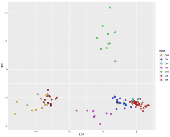

Figure 5.
Ordination of laboratory spectra on planes defined by LD components 1 to 4. Colors correspond to classified spectra. Letters indicate the actual mineral of those spectra for which the classification was wrong.
Classification accuracy was very high with data from the hyperspectral cameras, slightly lower when spectra of each camera were taken separately (Table 3): 95% for the FX10 (450–950 nm) and 94% for the FX17 (950–1650 nm). Instead, the classification accuracy was much lower (0.745) if only simulated RGB values were used. Confusion among minerals (Table 3) slightly increased for chalcopyrite, cassiterite, and malachite if only the FX10 spectra were considered, and for cassiterite and muscovite if only the FX17 spectra were considered. Confusion significantly increased if only RGB values were considered, in particular for cassiterite, which was always confused with wolframite, but also for chalcopyrite and wolframite. Interestingly, more modern classification methods such as SVM and RF achieved similar or even slightly lower performance than LDA (Table 4). Maximum accuracy of SVM was achieved with a dataset of nine components, sigma held constant to 0.1099153 and C = 32. Maximum accuracy of RF was achieved with a dataset of 10 PCs, with a subset of four (searched between 2 and 10) randomly selected at each node.
Table 3.
Confusion matrix of LDA classifications using laboratory spectra. Each value corresponds to the number of spectra observed as the mineral indicated by the row and predicted as indicated by the column. Spectral ranges: FX10_FX17: combined spectra (450–1650 nm); FX10 (450–950 nm); FX17 (950–1650 nm); RGB: Canon D60. Overall accuracies were 98.2%, 95.4%, 94.5%, and 72.7% in the same order. Acronyms in the columns correspond to the full names in the rows.
Table 4.
Accuracy values of different classification methods applied to laboratory spectra using the combined FX10FX17 dataset (450 nm–1650 nm). LDA, Linear Discriminant Analysis; SVM, Singular Vector Machine; RF, Random Forest.
4.2. Ground-Based Panoramic Hyperspectral Imaging of Simulated Mine Face
The grid search ran with EnMAP Box achieved a maximum accuracy for SVM with sigma = 0.1 and C = 1000, and with 350 trees and a subset of four randomly selected components at each node for RF. Each classification method applied to the FX17 hyperspectral image of the panel produced a map of the distribution of surface materials in the panel. Classification accuracy was lower than in the case of the laboratory spectra, but still high (Table 5): 90.6–91.4% if all classes were considered (Supplementary, Table S2), and 81.3–84.9% if only relevant materials (Table 6; 1163 pixels) were included. Overall accuracy was highest with the RF classifier.
Table 5.
Overall accuracy values of different classification methods applied to the FX17 hyperspectral image of the panel of hand samples. LDA, Linear Discriminant Analysis; SVM, Singular Vector Machines; RF, Random Forest. See the identity of “All classes” in Supplementary, Table S2 and of “Relevant classes” in Table 6.
Table 6.
Confusion matrix of main minerals in the Random Forest classification of the FX17 (950–1650 nm) hyperspectral image of the panel of hand samples. Each value corresponds to the number of spectra observed as the mineral indicated by the row and predicted as indicated by the column. Overall accuracy was 84.9% See Supplementary, Table S1 for the complete table.
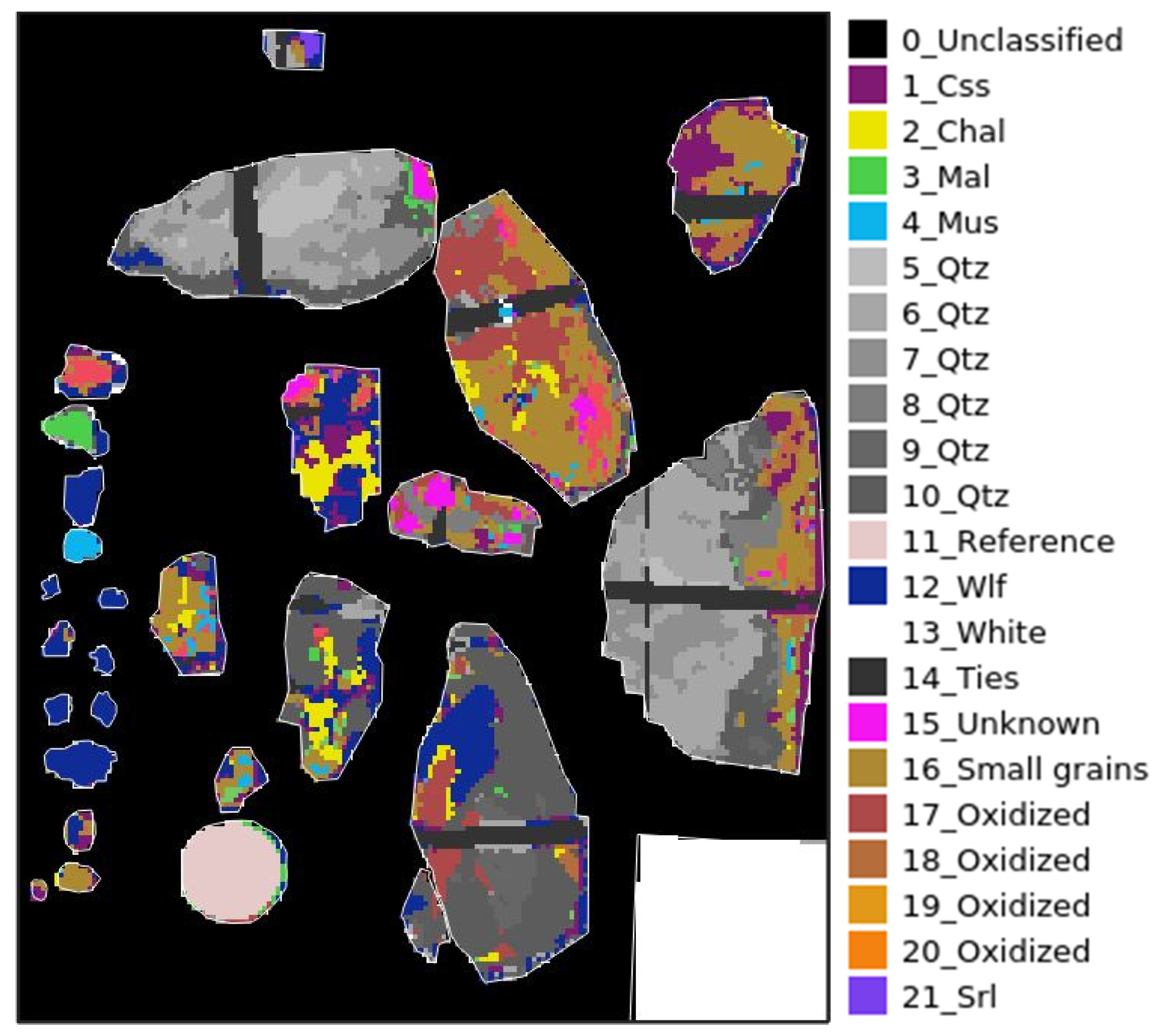
The confusion matrices (Table 6 and Supplementary, Table S2) revealed that, while a high accuracy was achieved for wolframite, cassiterite was too often confused with the former (in the case of the RF classification, a 37.5% of the all actual Cassiterite pixels were labelled as wolframite), but more rarely confused with any other material (10.6%). In other words, while the identification of wolframite was reliable, pixels identified as cassiterite could actually be either cassiterite or wolframite. As cassiterite and wolframite are the main ores in this mine, an operationally interesting product can result by lumping together both minerals in an “ore” category that reaches 94.8% of user’s accuracy and 93.9% of producer’s accuracy.
Figure 6 displays the combined result: all three classification methods agree on 53.8% of the study area, while at least two methods agreed in 87.5% of the study area. Within the training/validation polygons, the results of the three classifiers agreed in 90% of the area and, in that case, the agreed class was always correct.
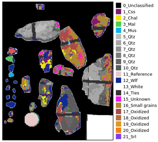
Figure 6.
Distribution of materials in the panel of hand samples by combining the result of all 3 classification methods. The agreed class was selected wherever results of 2 or 3 classification methods were coincident (33.7% and 53.8% of the total area, respectively), while the result of RF was kept for those pixels with no agreement (12.5%).
5. Discussion
An initial concern in this study was the fact that the used imaging hyperspectral systems were not covering the spectral range 2000–2500 nm, which is diagnostic for many geological materials (see, e.g., [4,9]). Imaging systems covering a wider spectral range have been used to acquire panoramic images in open pit mines [21,22,23,24,29,74,75,76]. To mention the most recent, Barton et al. [75] mapped different mixtures of carbonates, mica-rich muscovite mica, kaolinite, and gypsum in highwalls and outcrops using a system with 640 bands that integrates two sensors to cover from 400 to 2500 nm. Thiele et al. [76] used an equivalent (albeit much heavier) system to map an open-pit mine face in terms of oxidized materials, massive sulfides, Mg- and Fe-rich chlorite, two sericitic units, and shales. Nevertheless, our laboratory results very clearly indicated the strong discriminant power of the spectral ranges and signal quality of the much affordable FX10 and FX17 systems for the particular minerals of interest in this case of study. Undoubtedly, confusion could raise in the future with other, not considered, materials, but the ones we have included are those most common in the San Finx mine. Under these circumstances, the logistic criteria such as price, compactness, and robustness vs. extended spectral coverage must be considered in regard to deployment in a difficult environment such as a gallery mine. While a full system covering a wide spectral range is best for scientific research, practical applications call for the simplest system with the minimal set of characteristics for being successful in the given application. Actually, and according to our results, what is of more concern here is the fact that the 450–950 nm range was ignored in the field system that we tested for deployment in the actual gallery.
Three factors can be called to explain the decrease in accuracy between results obtained in the laboratory and in the simulation of gallery conditions: a narrower spectral range (from 450 to 1650 nm in the laboratory to 950–1650 nm in the gallery simulation), poorer illumination (dedicated illumination system in the laboratory stand vs. standard photography lighting system in the gallery simulation), and a coarser pixel size (0.224 mm vs. 2.6 mm) due to an increased camera–target distance. The narrower spectral range was a consequence of the logistic requirement of using one single hyperspectral imaging system in the gallery. While scanning with a compact system covering the 450 nm–1650 nm range (or more) would be better, our laboratory results indicated that, in this study, this was not a substantial factor. Illumination could be more challenging in the actual gallery than in the simulated conditions, but our experience in this study indicated that no parts of the image were critically under-illuminated, and that our methods to adjust moderate illumination unevenness were successful. Coarser pixels, instead, appear to be more responsible for the observed decreased accuracy. Large and uniform targets such as those of the standard reference have a crown of incorrect labels that put in evidence the effect of mixed pixels. While not so conspicuously, this effect was certainly present in other targets and must be more pervasive in those targets of smaller size, as in the case of cassiterite. Fragmentation probably makes the average size of ore minerals in the hand samples smaller than in the actual mine walls and, thus, the effect of pixel coarseness at producing spurious mixtures might have been over-emphasized in this study. Notwithstanding, the fact that the minimum size of ore patches being worth extracting can be as small as 1 cm2, indicates the interest of using a hyperspectral system with a higher spatial resolution for forthcoming studies in the actual mine gallery.
Spatial resolution can also be improved by the co-registration of hyperspectral images to conventional digital photography (“RGB”) and subsequent image fusion. Actually, a crude co-registration using 2D coordinates only was used in this study as an aid for photo-interpretation, but the correct co-registration requires 3D coordinates and, thus, generating a digital surface model [30,31,76], an involved task that will be worth addressing in the forthcoming study of the actual mine excavation face.
The co-registered RGB images of high resolution were also useful to add textural information to the classification processing, which usually involves a previous segmentation step. Texture is an important property to visually identify geological materials. Adding texture to the spectral information represents an opportunity to add image features to the pixel-based spectra; thus, taking better advantage of imaging systems for the identification of geological materials. Computing textural metrics in hyperspectral imagery is challenging, but specific methods are currently being developed [77,78,79].
6. Conclusions
Our results demonstrated the feasibility and interest of mapping materials of gallery mines in Sn–W deposits by analyzing hyperspectral images in the 950–1650 nm range through machine learning methods. In the laboratory study, spectral separability and overall accuracy were very high (95.4% with the 450–950 nm system; 94.5% with the 950–1650 nm system; 98.2% with the combined 450–1650 nm system). Results of three classification methods using the 450–1650 nm data were all very accurate: 98.2% for LDA and SVM, and 96.4% for RF. Instead, classification with a simulated RGB dataset resulted in high confusion among targets.
Our study of a simulated excavation face resulted in a classification map with a lower accuracy than in the laboratory, but still high: the RF method had the highest overall accuracy (84.9%), raising to 87.5% in a map combining all three classification methods. Cassiterite was too often confused with wolframite (user’s accuracy: 70%), but a lumped ore category (“wolframite or cassiterite”) achieved 94.9% user’s accuracy. These results encourage forthcoming studies deploying ground-based hyperspectral systems in the actual mine gallery to map the excavation face. A sequence of these maps at given time intervals as the excavation progress would improve the orebody assessment and document the structure of the deposit as a tomography, opening the way to detailed studies of the spatial distribution of ore mineralization and the evaluation of geologic models of the deposit.
Supplementary Materials
The following are available online at https://www.mdpi.com/article/10.3390/rs13163258/s1, Table S1: Description of target types in the panel of hand samples, Table S2: Accuracy metrics of all panel materials: LDA, SVM and RF classifications.
Author Contributions
Conceptualization, A.L., D.M., J.I.-I. and J.-L.F.-T.; methodology, A.L.; software, A.L. and G.B.; validation, A.L., E.G. and G.B.; formal analysis, A.L. and G.B.; investigation, A.L., E.G. and G.B.; resources, D.M.; data curation, A.L. and E.G.; writing—original draft preparation, A.L.; writing—review and editing, J.-L.F.-T. and J.I.-I.; visualization, A.L. and G.B.; supervision, A.L.; project administration, J.I.-I.; funding acquisition, D.M. All authors have read and agreed to the published version of the manuscript.
Funding
EIT RawMaterials supported this research within the framework of the iTARG3T (Innovative targeting & processing of W–Sn–Ta–Li ores: towards EU’s self-supply) project nb. 18036.
Institutional Review Board Statement
Not applicable.
Informed Consent Statement
Not applicable.
Data Availability Statement
The data presented in this study are available on request from the corresponding author.
Acknowledgments
We thank Valoriza Minería, in particular Ivan Losada, for providing the mine hand samples, as well as Marc Campeny-Crego and Fernando Tornos for their useful comments. We also would like to acknowledge the anonymous reviewers for their valuable suggestions. Hyperspectral imaging was conducted by the Laboratory of Hyperspectral Imaging of GeoSciences Barcelona, CSIC.
Conflicts of Interest
The authors declare no conflict of interest. The funders had no role in the design of the study; in the collection, analyses, or interpretation of data; in the writing of the manuscript, or in the decision to publish the results.
References
- Goetz, A.F.H.; Vane, G.; Solomon, J.E.; Rock, B.N. Imaging Spectrometry for Earth Remote Sensing. Science 1985, 228, 1147–1153. [Google Scholar] [CrossRef] [PubMed]
- Amigo Rubio, J.M. Hyperspectral Imaging; Data Handling in Science and Technology; Elsevier: Amsterdam, The Netherlands, 2020; ISBN 978-0-444-63977-6. [Google Scholar]
- Milton, E.J. Principles of field spectroscopy. Int. Remote Sens. 1987, 8, 1807–1827. [Google Scholar] [CrossRef]
- Clark, R.N. Spectroscopy of Rocks and Minerals, and Principles of Spectroscopy. In Remote Sensing for the Earth Sciences: Manual of Remote Sensing; Rencz, A.N., Ed.; John Wiley & Sons: New York, NY, USA, 1999; Volume 3, pp. 3–52. [Google Scholar]
- Hunt, G.R.; Salisbury, J.W. Visible and Near-Infrared Spectra of Minerals and Rocks: I Silicate Minerals. Mod. Geol. 1970, 1, 283–300. [Google Scholar]
- Hunt, G.R. Spectral signatures of particulate minerals in the visible and near infrared. Geophysics 1977, 42, 501–513. [Google Scholar] [CrossRef] [Green Version]
- Clark, R.N.; King, T.V.; Klejwa, M.; Swayze, G.A.; Vergo, N. High spectral resolution reflectance spectroscopy of minerals. J. Geophys. Res. Solid Earth 1990, 95, 12653–12680. [Google Scholar] [CrossRef] [Green Version]
- van der Meer, F.D.; van der Werff, H.M.A.; van Ruitenbeek, F.J.A.; Hecker, C.A.; Bakker, W.H.; Noomen, M.F.; van der Meijde, M.; Carranza, E.J.M.; de Smeth, J.B.; Woldai, T. Multi- and hyperspectral geologic remote sensing: A review. Int. J. Appl. Earth Obs. Geoinf. 2012, 14, 112–128. [Google Scholar] [CrossRef]
- Peyghambari, S.; Zhang, Y. Hyperspectral Remote Sensing in Lithological Mapping, Mineral Exploration, and Environmental Geology: An Updated Review. JARS 2021, 15, 031501. [Google Scholar] [CrossRef]
- Bedell, R.; Crósta, A.P.; Grunski, E. Remote Sensing and Spectral Geology; Society of Economic Geologists: Westminster, CO, USA, 2009; ISBN 978-1-934969-13-7. [Google Scholar]
- Pour, A.B.; Zoheir, B.; Pradhan, B.; Hashim, M. Editorial for the Special Issue: Multispectral and Hyperspectral Remote Sensing Data for Mineral Exploration and Environmental Monitoring of Mined Areas. Remote Sens. 2021, 13, 519. [Google Scholar] [CrossRef]
- Gupta, R.P. Imaging Spectroscopy. In Remote Sensing Geology; Springer: Berlin/Heidelberg, Germany, 2018; pp. 203–219. ISBN 978-3-662-55874-4. [Google Scholar]
- Riaza, A.; Buzzi, J.; García-Meléndez, E.; Vázquez, I.; Bellido, E.; Carrère, V.; Müller, A. Pyrite mine waste and water mapping using Hymap and Hyperion hyperspectral data. Environ. Earth Sci. 2012, 66, 1957–1971. [Google Scholar] [CrossRef]
- Buzzi, J.; Riaza, A.; García-Meléndez, E.; Weide, S.; Bachmann, M. Mapping Changes in a Recovering Mine Site with Hyperspectral Airborne HyMap Imagery (Sotiel, SW Spain). Minerals 2014, 4, 313. [Google Scholar] [CrossRef] [Green Version]
- Song, W.; Song, W.; Gu, H.; Li, F. Progress in the Remote Sensing Monitoring of the Ecological Environment in Mining Areas. Int. J. Environ. Res. Public Health 2020, 17, 1846. [Google Scholar] [CrossRef] [Green Version]
- Bolin, B.J.; Moon, T.S. Sulfide detection in drill core from the Stillwater Complex using visible/near-infrared imaging spectroscopy. Geophysics 2003, 68, 1561–1568. [Google Scholar] [CrossRef]
- Kruse, F.A.; Bedell, R.L.; Taranik, J.V.; Peppin, W.A.; Weatherbee, O.; Calvin, W.M. Mapping alteration minerals at prospect, outcrop and drill core scales using imaging spectrometry. Int. J. Remote Sens. 2012, 33, 1780–1798. [Google Scholar] [CrossRef] [Green Version]
- Mathieu, M.; Roy, R.; Launeau, P.; Cathelineau, M.; Quirt, D. Alteration mapping on drill cores using a HySpex SWIR-320m hyperspectral camera: Application to the exploration of an unconformity-related uranium deposit (Saskatchewan, Canada). J. Geochem. Explor. 2017, 172, 71–88. [Google Scholar] [CrossRef]
- Coulter, D.W.; Zhou, X.; Harris, P.D. Advances in Spectral Geology and Remote Sensing: 2008–2017. In Proceedings of the Exploration 17: Sixth Decennial International Conference on Mineral Exploration; Tschirhart, V., Thomas, M.D., Eds.; Decennial Mineral Exploration Conferences: Toronto, ON, Canada, 2017; pp. 23–50. [Google Scholar]
- Murphy, R.J.; Monteiro, S.T.; Schneider, S. Evaluating Classification Techniques for Mapping Vertical Geology Using Field-Based Hyperspectral Sensors. IEEE Trans. Geosci. Remote Sens. 2012, 50, 3066–3080. [Google Scholar] [CrossRef]
- Ramanaidou, E.R.; Wells, M.A. Hyperspectral Imaging of Iron Ores. In Proceedings of the 10th International Congress for Applied Mineralogy (ICAM); Broekmans, M.A.T.M., Ed.; Springer: Berlin/Heidelberg, Germany, 2012; pp. 575–580. ISBN 978-3-642-27681-1. [Google Scholar]
- Okyay, Ü.; Khan, S.; Lakshmikantha, M.; Sarmiento, S. Ground-Based Hyperspectral Image Analysis of the Lower Mississippian (Osagean) Reeds Spring Formation Rocks in Southwestern Missouri. Remote Sens. 2016, 8, 1018. [Google Scholar] [CrossRef] [Green Version]
- Okyay, U.; Khan, S.D. Spatial Co-Registration and Spectral Concatenation of Panoramic Ground-Based Hyperspectral Images. Photogramm. Eng. Remote Sens. 2018, 84, 781–790. [Google Scholar] [CrossRef]
- Krupnik, D.; Khan, S. Close-range, ground-based hyperspectral imaging for mining applications at various scales: Review and case studies. Earth-Sci. Rev. 2019, 198, 102952. [Google Scholar] [CrossRef]
- Pirard, E. Multispectral imaging of ore minerals in optical microscopy. Mineral. Mag. 2004, 68, 323–333. [Google Scholar] [CrossRef]
- Pirard, E.; Bernhardt, H.-J.; Catalina, J.-C.; Brea, C.; Segundo, F.; Castroviejo, R. From Spectrophotometry to Multispectral Imaging of Ore Minerals in Visible and Near Infrared (VNIR) Microscopy. In Proceedings of the 9th International Congress for Applied Mineralogy (ICAM 2008), Brisbane, Australia, 8–10 September 2008; ISBN 978-1-920806-86-6. [Google Scholar]
- Berrezueta, E.; Ordóñez-Casado, B.; Bonilla, W.; Banda, R.; Castroviejo, R.; Carrión, P.; Puglla, S. Ore Petrography Using Optical Image Analysis: Application to Zaruma-Portovelo Deposit (Ecuador). Geosciences 2016, 6, 30. [Google Scholar] [CrossRef] [Green Version]
- López-Benito, A.; Catalina, J.C.; Alarcón, D.; Grunwald, Ú.; Romero, P.; Castroviejo, R. Automated ore microscopy based on multispectral measurements of specular reflectance. A comparative study of some supervised classification techniques. Miner. Eng. 2020, 146, 106136. [Google Scholar] [CrossRef]
- Murphy, R.J.; Taylor, Z.; Schneider, S.; Nieto, J. Mapping clay minerals in an open-pit mine using hyperspectral and LiDAR data. Eur. J. Remote Sens. 2015, 48, 511–526. [Google Scholar] [CrossRef]
- Jakob, S.; Zimmermann, R.; Gloaguen, R. The Need for Accurate Geometric and Radiometric Corrections of Drone-Borne Hyperspectral Data for Mineral Exploration: MEPHySTo—A Toolbox for Pre-Processing Drone-Borne Hyperspectral Data. Remote Sens. 2017, 9, 88. [Google Scholar] [CrossRef] [Green Version]
- Lorenz, S.; Salehi, S.; Kirsch, M.; Zimmermann, R.; Unger, G.; Vest Sørensen, E.; Gloaguen, R. Radiometric Correction and 3D Integration of Long-Range Ground-Based Hyperspectral Imagery for Mineral Exploration of Vertical Outcrops. Remote Sens. 2018, 10, 176. [Google Scholar] [CrossRef] [Green Version]
- Kruse, F.A.; Lefkoff, A.B.; Boardman, J.; Heidebrecht, K.; Shapiro, A.; Barloon, P.J.; Goetz, A. The spectral image processing system (SIPS) interactive visualization and analysis of imaging spectrometer data. Remote Sens. Environ. 1993, 44, 145–163. [Google Scholar] [CrossRef]
- Varshney, P.K.; Arora, M. Advanced Image Processing Techniques for Remotely Sensed Hyperspectral Data; Springer: Berlin/Heidelberg, Germany, 2004; ISBN 978-3-642-06001-4. [Google Scholar]
- van der Linden, S.; Rabe, A.; Held, M.; Jakimow, B.; Leitão, P.; Okujeni, A.; Schwieder, M.; Suess, S.; Hostert, P. The EnMAP-Box—A Toolbox and Application Programming Interface for EnMAP Data Processing. Remote Sens. 2015, 7, 1249. [Google Scholar] [CrossRef] [Green Version]
- Kokaly, R.; Graham, G.E.; Hoefen, T.M.; Kelley, K.D.; Johnson, M.R.; Hubbard, B.E.; Buchhorn, M.; Prakash, A. Multiscale hyperspectral imaging of the Orange Hill Porphyry Copper Deposit, Alaska, USA, with laboratory-, field-, and aircraft-based imaging spectrometers. In Proceedings of Exploration 17: Sixth Decennial International Conference on Mineral Exploration; Tschirhart, V., Thomas, M.D., Eds.; Decennial Mineral Exploration Conferences: Toronto, ON, Canada, 2017; pp. 923–943. [Google Scholar]
- Camps-Valls, G. Machine learning in remote sensing data processing. In Proceedings of the 2009 IEEE International Workshop on Machine Learning for Signal Processing, Grenoble, France, 1–4 September 2009; pp. 1–6. [Google Scholar]
- Plaza, A.; Benediktsson, J.A.; Boardman, J.W.; Brazile, J.; Bruzzone, L.; Camps-Valls, G.; Chanussot, J.; Fauvel, M.; Gamba, P.; Gualtieri, A.; et al. Recent advances in techniques for hyperspectral image processing. Remote Sens. Environ. 2009, 113, S110–S122. [Google Scholar] [CrossRef]
- Cracknell, M.J.; Reading, A.M. Geological mapping using remote sensing data: A comparison of five machine learning algorithms, their response to variations in the spatial distribution of training data and the use of explicit spatial information. Comput. Geosci. 2014, 63, 22–33. [Google Scholar] [CrossRef] [Green Version]
- Krupnik, D.; Khan, S.D. High-Resolution Hyperspectral Mineral Mapping: Case Studies in the Edwards Limestone, Texas, USA and Sulfide-Rich Quartz Veins from the Ladakh Batholith, Northern Pakistan. Minerals 2020, 10, 967. [Google Scholar] [CrossRef]
- Simancas, J.F. Variscan Cycle. In The Geology of Iberia: A Geodynamic Approach: Volume 2: The Variscan Cycle; Quesada, C., Oliveira, J.T., Eds.; Regional Geology Reviews; Springer: Cham, Switzerland, 2019; pp. 1–25. ISBN 978-3-030-10519-8. [Google Scholar]
- Ruiz Mora, J.E. Mineralizaciones estannovolframíferas en Noia y Lousame: Estudio previo. Cadernos Lab. Xeol. Laxe Revista Xeol. Galega Hercinico Penins. 1982, 3, 595–622. [Google Scholar]
- Mangas Viñuela, J.; Arribas Moreno, A. Estudio de las inclusiones fluidas atrapadas en cristales de casiterita y cuarzo del yacimiento de San Finx (La Coruña, España). Bol. Sociedad Esp. Mineral. 1989, 12, 241–259. [Google Scholar]
- Rodríguez-Terente, L.-M.; Fernández-González, M.-Á.; Losada-García, I. Estudio cristalográfico de la Bertrandita de las minas de San Finx (A Coruña, España). Macla 2014, 19, 1–2. [Google Scholar]
- Llana-Funez, S. La Estructura de la Unidad de Malpica-Tui (Cordillera Varisca en Iberia); Universidad de Oviedo: Oviedo, Spain, 2001; ISBN 84-7840-431-7. [Google Scholar]
- R Core Team. R: A Language and Environment for Statistical Computing; R Foundation for Statistical Computing: Vienna, Austria, 2018. [Google Scholar]
- Hijmans, R.J. Raster: Geographic Data Analysis and Modeling. 2018. Available online: https://cran.r-project.org/web/packages/raster/index.html (accessed on 19 April 2021).
- Bivand, R.; Keitt, T.; Rowlingson, B. Rgdal: Bindings for the “Geospatial” Data Abstraction Library. 2019. Available online: https://cran.r-project.org/web/packages/rgdal/index.html (accessed on 19 April 2021).
- Leutner, B.; Horning, N.; Schwalb-Willmann, J. RStoolbox: Tools for Remote Sensing Data Analysis. 2019. Available online: https://cran.r-project.org/web/packages/RStoolbox/RStoolbox.pdf (accessed on 19 April 2021).
- O’Brien, J. GdalUtilities: R Wrappers for the GDAL Utilities Executables Shipped with Sf. 2018. Available online: https://cran.r-project.org/web/packages/gdalUtilities/index.html (accessed on 19 April 2021).
- Reudenbach, C. Link2GI: Linking Geographic Information Systems, Remote Sensing and Other Command Line Tools. 2019. Available online: https://cran.r-project.org/web/packages/link2GI/link2GI.pdf (accessed on 19 April 2021).
- GDAL/OGR contributors. GDAL/OGR Geospatial Data Abstraction Software Library; Open Source Geospatial Foundation: Chicago, IL, USA, 2019. [Google Scholar]
- Grizonnet, M.; Michel, J.; Poughon, V.; Inglada, J.; Savinaud, M.; Cresson, R. Orfeo ToolBox: Open source processing of remote sensing images. Open Geospat. Data Softw. Stand. 2017, 2, 15. [Google Scholar] [CrossRef] [Green Version]
- McInerney, D.; Kempeneers, P. Pktools. In Open Source Geospatial Tools: Applications in Earth Observation; Earth Systems Data and Models; McInerney, D., Kempeneers, P., Eds.; Springer: Cham, Switzerland, 2015; pp. 173–197. ISBN 978-3-319-01824-9. [Google Scholar]
- Lowe, D.G. Object recognition from local scale-invariant features. In Proceedings of the Seventh IEEE International Conference on Computer Vision, Kerkyra, Greece, 20–27 September 1999; Volume 2, pp. 1150–1157. [Google Scholar]
- EnMAP Core Science Team. EnMAP-Box 3-A QGIS Plugin to Process and Visualize Hyperspectral Remote Sensing Data. 2019. Available online: https://enmap-box.readthedocs.io (accessed on 19 April 2021).
- QGIS.org. QGIS Geographic Information System. QGIS Association, 2021. Available online: http://www.qgis.org (accessed on 19 April 2021).
- Kokaly, R.F.; Clark, R.N.; Swayze, G.A.; Livo, K.E.; Hoefen, T.M.; Pearson, N.C.; Wise, R.A.; Benzel, W.M.; Lowers, H.A.; Driscoll, R.L.; et al. USGS Spectral Library Version 7; Data Series; U.S. Geological Survey: Reston, VA, USA, 2017; p. 68.
- Baldridge, A.M.; Hook, S.J.; Grove, C.I.; Rivera, G. The ASTER spectral library version 2.0. Remote Sens. Environ. 2009, 113, 711–715. [Google Scholar] [CrossRef]
- Meerdink, S.K.; Hook, S.J.; Roberts, D.A.; Abbott, E.A. The ECOSTRESS spectral library version 1.0. Remote Sens. Environ. 2019, 230, 111196. [Google Scholar] [CrossRef]
- Richards, J.A.; Jia, X. Remote Sensing Digital Image Analysis: An Introduction, 4th ed.; Springer: Berlin/Heidelberg, Germany, 2005; ISBN 3-540-25128-6. [Google Scholar]
- Jiang, J.; Liu, D.; Gu, J.; Susstrunk, S. What is the space of spectral sensitivity functions for digital color cameras? In Proceedings of the 2013 IEEE Workshop on Applications of Computer Vision (WACV), Washington, DC, USA, 15–17 January 2013; IEEE: Clearwater Beach, FL, USA, 2013; pp. 168–179. [Google Scholar]
- Venables, W.N.; Ripley, B.D. Modern Applied Statistics with S, 4th ed.; Springer: New York, NY, USA, 2002. [Google Scholar]
- Meyer, D.; Dimitriadou, E.; Hornik, K.; Weingessel, A.; Leisch, F. e1071: Misc Functions of the Department of Statistics, Probability Theory Group (Formerly: E1071); TU Wien: Vienna, Austria, 2020. [Google Scholar]
- Liaw, A.; Wiener, M. Classification and Regression by randomForest. R News 2002, 2, 18–22. [Google Scholar]
- Kuhn, M. Building Predictive Models in R Using the caret Package. J. Stat. Softw. 2008, 28, 149119. [Google Scholar] [CrossRef] [Green Version]
- Castle, M.; Keller, J. Rolling Ball Background Subtraction. Available online: https://imagej.net/plugins/rolling-ball.html (accessed on 19 April 2021).
- Schindelin, J.; Arganda-Carreras, I.; Frise, E.; Kaynig, V.; Longair, M.; Pietzsch, T.; Preibisch, S.; Rueden, C.; Saalfeld, S.; Schmid, B.; et al. Fiji: An open-source platform for biological-image analysis. Nat. Meth. 2012, 9, 676–682. [Google Scholar] [CrossRef] [PubMed] [Green Version]
- James, G.; Witten, D.; Hastie, T.; Tibshirani, R. An Introduction to Statistical Learning with Applications in R Springer Texts in Statistics, 1st ed.; Springer: New York, NY, USA, 2013; ISBN 978-1-4614-7138-7. [Google Scholar]
- Pedregosa, F.; Varoquaux, G.; Gramfort, A.; Michel, V.; Thirion, B.; Grisel, O.; Blondel, M.; Prettenhofer, P.; Weiss, R.; Dubourg, V.; et al. Scikit-learn: Machine Learning in Python. J. Mach. Learn. Res. 2011, 12, 2825–2830. [Google Scholar]
- Kuhn, M.; Johnson, K. Applied Predictive Modeling; Springer: New York, NY, USA, 2013; ISBN 978-1-4614-6848-6. [Google Scholar]
- Congalton, R.G. A review of assessing the accuracy of classifications of remotely sensed data. Remote Sens. Environ. 1991, 37, 35–46. [Google Scholar] [CrossRef]
- Maxwell, A.E.; Warner, T.A. Thematic Classification Accuracy Assessment with Inherently Uncertain Boundaries: An Argument for Center-Weighted Accuracy Assessment Metrics. Remote Sens. 2020, 12, 1905. [Google Scholar] [CrossRef]
- Goutte, C.; Gaussier, E. A Probabilistic Interpretation of Precision, Recall and F-Score, with Implication for Evaluation. In Advances in Information Retrieval; Lecture Notes in Computer Science; Losada, D.E., Fernández-Luna, J.M., Eds.; Springer: Berlin/Heidelberg, Germany, 2005; Volume 3408, pp. 345–359. ISBN 978-3-540-25295-5. [Google Scholar]
- Fraser, S.; Whitbourn, L.B.; Yang, K.; Ramanaidou, E.; Connor, P.; Poropat, G.; Soole, P.; Mason, P.; Coward, D.; Philips, R. Mineralogical Face-Mapping Using Hyperspectral Scanning for Mine Mapping and Control. In Proceedings of the Australasian Institute of Mining and Metallurgy Publication Series; Australasian Institute of Mining and Metallurgy: Darwin, Australia, 2006; Volume AusIMM, pp. 227–232. [Google Scholar]
- Barton, I.F.; Gabriel, M.J.; Lyons-Baral, J.; Barton, M.D.; Duplessis, L.; Roberts, C. Extending geometallurgy to the mine scale with hyperspectral imaging: A pilot study using drone- and ground-based scanning. Min. Metall. Explor. 2021, 38, 799–818. [Google Scholar] [CrossRef]
- Thiele, S.T.; Lorenz, S.; Kirsch, M.; Cecilia Contreras Acosta, I.; Tusa, L.; Herrmann, E.; Möckel, R.; Gloaguen, R. Multi-scale, multi-sensor data integration for automated 3-D geological mapping. Ore Geol. Rev. 2021, 136, 104252. [Google Scholar] [CrossRef]
- Li, P.; Xiao, X. Multispectral image segmentation by a multichannel watershed-based approach. Int. J. Remote Sens. 2007, 28, 4429–4452. [Google Scholar] [CrossRef]
- Gao, F.; Wang, Q.; Dong, J.; Xu, Q. Spectral and Spatial Classification of Hyperspectral Images Based on Random Multi-Graphs. Remote Sens. 2018, 10, 1271. [Google Scholar] [CrossRef] [Green Version]
- Camps-Valls, G.; Shervashidze, N.; Borgwardt, K. Spatio-Spectral Remote Sensing Image Classification With Graph Kernels. IEEE Geosci. Remote Sens. Lett. 2010, 7, 741–745. [Google Scholar] [CrossRef]
Publisher’s Note: MDPI stays neutral with regard to jurisdictional claims in published maps and institutional affiliations. |
© 2021 by the authors. Licensee MDPI, Basel, Switzerland. This article is an open access article distributed under the terms and conditions of the Creative Commons Attribution (CC BY) license (https://creativecommons.org/licenses/by/4.0/).