Oil Spill Detection in SAR Images Using Online Extended Variational Learning of Dirichlet Process Mixtures of Gamma Distributions

Abstract

In this paper, we propose a Dirichlet process (DP) mixture model of Gamma distributions, which is an extension of the finite Gamma mixture model to the infinite case. In particular, we propose a novel online nonparametric Bayesian analysis method based on the infinite Gamma mixture model where the determination of the number of clusters is bypassed via an infinite number of mixture components. The proposed model is learned via an online extended variational Bayesian inference approach in a flexible way where the priors of model’s parameters are selected appropriately and the posteriors are approximated effectively in a closed form. The online setting has the advantage to allow data instances to be treated in a sequential manner, which is more attractive than batch learning especially when dealing with massive and streaming data. We demonstrated the performance and merits of the proposed statistical framework with a challenging real-world application namely oil spill detection in synthetic aperture radar (SAR) images.

1. Introduction

The use of statistical machine learning has proliferated in many fields, especially to solve a broad range of problems ranging from signal processing, speech recognition, to geosciences and remote sensing where strong models are needed to apply statistical methodology. In the case of geosciences and remote sensing, for instance, statistical machine learning techniques have been deployed successfully in a variety of problems and applications in many parts of the earth system and beyond [1]. In particular, images modeling (e.g., SAR images) has received much attention due to its importance and applications in real world nature tasks related to land, climate, disturbance attribution, vegetation dynamics, urbanization, etc.

Among the probabilistic generative models, the so-named finite mixtures have been successfully applied due to their capability to represent large-scale complex probability densities and to offer a principled way for analyzing missing data [2,3]. Mixture models provide, in general, a formal approach to unsupervised learning and allow, in particular, to select the optimal number of clusters for a given dataset. This fact has been largely detailed in the literature (see, for example, [4,5]). This growing interest has led to developing several fascinating and flexible mixture models such as Gaussian-based mixture models (GMM) which have became popular even though they are not the most appropriate for fitting complex non-Gaussian shapes [6,7]. To deal with conventional GMM limitations, many other alternatives, such as Gamma (GaMM) mixtures [8,9,10,11], have shown to perform significantly better than GMM [12] thanks to its compact analytical form which is able to cover long-tailed distributions and to approximate data with outliers. Thus, motivated by the flexibility and good performance obtained with Gamma distribution, we will focus here on investigating Gamma-based mixture model for SAR images classification. We are mainly motivated by the excellent results that Gamma mixture has provided, thanks to its flexibility, for SAR images analysis in many applications such as target detection and discrimination, target recognition and surface classification, oil spill detection, noise reduction, etc. [10]. In this paper, we will focus mainly on oil spill detection.

The most challenging problem within finite mixture models is the estimation of the number of clusters that best describes the data without over- or under-fitting [13,14]. In the statistical learning context, this problem is solved using frequentist approach (i.e., maximum likelihood (ML)) within some criteria (ex. Akaike’s Information Criterion, Minimum Description Length, Minimum Message Length, etc) [15,16]. It is noteworthy that the evaluation of these criteria for many clusters using ML method is very costly in terms of calculation. In addition, all parameters are supposed fixed and the inference process is based mainly on the likelihood of data which leads to convergence isssues. An alternative way to tackle the issue of selecting accurately the number of clusters is via nonparametric Bayesian inference using for instance Dirichlet process (DP) [17]. In this case, the number of clusters may increase as more data are observed. This property makes DP extremely useful in exploratory data analysis. Thus, the assumption of an infinite number of components allows to avoid the problems of over- and under-fitting. Dirichlet processes (DP) mixtures have become a popular choice for various machine learning applications thanks to effective sampling techniques such as Markov chain Monte Carlo (MCMC) [18,19]. Despite the fact that MCMC yields good performance, it is frequently limited to small-scale problems and computationally intensive [20].

An interesting alternative, to both frequentist and Bayesian methods, which has provided promising performance, is variational Bayes learning [15,21]. Variational inference has the advantage to find optimal approximate posterior distributions by minimizing Kullback–Leibler (KL) divergence, or as maximizing evidence lower bound. Recently, an extended variational inference (EVI) was proposed [8] and has shown to be efficient for minimizing the KL divergence and for tackling the estimation problem. In this work, we go a step further by developing an infinite mixture model based on Gamma distribution via Dirichlet process prior, and then we propose to exploit the merits found recently by the extended variational framework [8] to learn the developed mixture model (InGaMM-eV) in an online manner. Furthermore, it is possible to estimate all parameters in closed forms. Moreover, compared to batch algorithms, online learning is more effective and helpful especially when processing big and streaming data [22] which can be crucial in SAR images analysis to allow continuous monitoring of the earth’s surface. It is noteworthy also that many SAR satellite missions have accumulated repeated observations over the last decades and processing these data in an online manner could offer ease of use and solutions to some challenging problems (e.g., change detection [23]). Thus, an effective online extended variational framework of Dirichlet process mixtures of Gamma distributions is developed using stick-breaking representation. As a result, the number of clusters is selected appropriately, the model’s parameters are learned in a closed form, and the issue of under-fitting is solved by deriving a model with an unlimited complexity.

The rest of this manuscript is presented as follows. We review some relevant works related to oil spill detection in Section 2. The details of extending the finite Gamma mixture to infinite case are given in Section 3. The principles of our implemented nonparametric variational learning algorithm of infinite Gamma mixture are provided in Section 4 and Section 5. Section 6 is devoted to discuss the results obtained from experiments. Finally, the paper is concluded with some future works.

2. Related Research Work

Oil pollution is a major ocean disaster and environmental threat to coastal ecosystems which has been recently highlighted by several tankers accidents around the world. Accidents on offshore oil platforms, refineries, and pipeline can cause serious oil spills. However, these accidents represent only 5% of the total oil pollution worldwide, and 95% are caused by illegal discharges by ships that prefer to dispose, cheaply, of oil residues in their tanks (according to many studies such as the European Space Agency) [24,25,26]. Oil pollution may result from several sources such as industrial discharges, oil production, natural oil seepage, and urban runoff. Natural slicks are of bacterial or biological decomposition or geological origin. Oil spills can devastate naval life as well as harm humans and animals by reducing dramatically air-sea exchanges processes, such as surface evaporation. Oil spills are then of great public, political and scientific concern. Therefore, there is an urgent need to monitor and detect oil spills on ocean so as to facilitate government decision making. The detection of these oil spills is considered an important and challenging problem to effectively conduct countermeasures. An effective approach is the use of satellites which provide radar images of the sea surface ($500\times 500$ km² in a single image). Satellites radar images supply an occasion to monitor coastal waters day and night, regardless of weather conditions allowing an early warning of oil spills. Moreover, satellite detection is well adapted to this kind of problems by producing images of difficult access areas [24]. Among different satellite imagery technologies, active microwave sensors such as synthetic aperture radar (SAR), has been frequently investigated for remote sensing of oil pollution [27]. The synthetic aperture radar emits and receives radio wave in order to acquire a representation of the target scene. Detecting oil spill in SAR images (as shown in Figure 1) is very complex procedure that involves many steps [26].

For several decades, extensive works have been provided [27,29,30] to distinguish oil slicks from natural biogenic slicks via analyzing satellite radar images. Most of conventional oil slick (or dark objects) detection procedures are carried out in three steps: (1) a pre-segmentation of dark spot, (2) the extraction of dark spot feature, and (3) a classification step of these dark spots. Some early and recent review articles summarize different oil slick detection methods [26,28,31]. These reviews state that most methods are based on using statistical patterns to discriminate between oil slicks and look-alikes under varying conditions. They conclude also that the automatic and accurate discrimination between oil spills and look-alikes is a challenging problem and need more investigations in the future. On the other side, a lot of efforts have been devoted to apply classic classifiers and descriptive statistical approaches learned from training data [25,30,32,33,34]. These works rely on highly trained human operators to asses and verify each region in a given SAR image. In [33], authors proposed a one-class based approach for image classification to detect oil-spill. First of all, a preprocessing step is used to identify related areas to oil spills. A feature selection step to select relevant features is also performed given that the contrast between spill’s region and the surrounding regions depends on the type and amount of oil and other environmental factors (i.e., wave height, wind speed, and sea). Finally, a one-class classifier is used to detect oil spills. A geometric level-set based segmentation method of oil spills and illegal oil discharges was developed in [35]. According to this work the regions in SAR images can be classified into pure oil spills or look-alikes on the basis of the following measurements: orientation, area, shape complexity, perimeter, eccentricity, and mean border gradient. In [36], a region-based method was also proposed. It involves both conventional detection theory and image segmentation techniques (such as N-nearest-neighbor) to have more accurate results. In [37], authors developed an adaptive thresholding-based algorithm to classify each slick as oil or look-alike. Here, involved features are derived from shape (slick complexity, width, area, moment), slick surroundings, contrast (slick local contrast, border gradient, smoothness contrast), and slick homogeneity. Their algorithms have been trained on two datasets, namely Radarsat and Envisat Advanced Synthetic Aperture Radar (ASAR) images. Fuzzy classifiers have been also used in [38] to identify all possible oil spills (dark patterns) in SAR images. A set of operations based on the fuzzy theory are used to establish the likeness of each candidate to be an oil spill or not. In the last few years, artificial neural network algorithms have been broadly applied in the context of remote sensing image segmentation and classification. Indeed, authors in [39,40,41,42,43] proposed different neural network-based methods (like CNN and Deep NN) in order to improve oil spill detection and classification. Some other notable interesting CNN-based oil spill detection and classification frameworks include the works in [44,45].

While considerable progress has been made in this field over the past few years, designing more robust tools still needs wide amounts of specialized knowledge and manual work. The goal here is to propose a method based on a nonparametric Bayesian model (infinite model) as well as to learn it using variational inference. Our main contributions are summarized as follow: First, we start by extending the finite Gamma mixture to the infinite case via a nonparametric Dirichlet process prior such that the problem of selecting the suitable number of clusters is solved fashionably. Then, we investigate the developed approach for remote sensing image classification. Indeed, after extracting effective features as in [46], we shall focus on modelling and classifying oil spills and other similar sea surface features using the infinite mixture model. The merits of our approach have been demonstrated using real datasets.

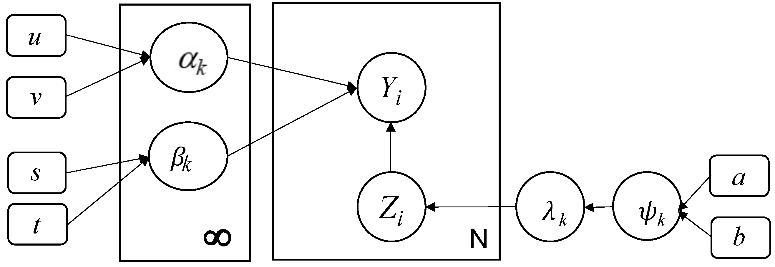
3. Statistical Model Specification

In this section, we present our developed variational learning approach based on the infinite Gamma mixture model.

3.1. Finite Gamma Mixture Model

Let’s denote by $\mathcal{Y}$ our observed data such as $\mathcal{Y}=\{{\overrightarrow{Y}}_1,\dots ,{\overrightarrow{Y}}_N\}$, where each $\overrightarrow{Y_i}=(Y_{i1},Y_{i2},\dots ,Y_{iD})$ is a D-dimensional positive vector. These feature vectors are supposed to be drawn from a mixture of Gamma distributions with parameter $\mathrm{\Theta }$. Let M denotes the number of mixture’s components. ${\overrightarrow{Y}}_i$ ($i=1,\dots ,N$) are independent and identically distributed (iid). The density function of multi-dimensional Gamma distribution is defined as follows:

$$p({\overrightarrow{Y}}_i\mid \theta )=\prod _{d=1}^D\frac{{({\beta }_d)}^{{\alpha }_d}{Y}_{id}^{{\alpha }_d-1}{e}^{-{\beta }_d{Y}_{id}}}{\mathrm{\Gamma }({\alpha }_d)}$$

(1)

where $\theta =\{{\alpha }_d,{\beta }_d\}$ is the set of parameters of the distribution such that ${\alpha }_d$ denotes the shape and ${\beta }_d$ the location parameter. Here, $\mathrm{\Gamma }(.)$ is the Gamma function which is given as: $\mathrm{\Gamma }(x)={\int }_0^{\infty }{s}^{x-1}{e}^{-s}ds$.

Suppose that the D-dimensional random vector ${\overrightarrow{Y}}_i$ (observed data) is drawn from a finite mixture of Gamma (GaMM) distributions and consisting of M components which is established to model the data with different shapes. The probability density function (pdf) of a GaMM is then given as:

$$p(\overrightarrow{Y}\mid \mathrm{\Theta })=p(\overrightarrow{Y}\mid \overrightarrow{\alpha },\overrightarrow{\beta },\overrightarrow{\pi })=\prod _{i=1}^N\sum _{j=1}^M{\pi }_{j}p({\overrightarrow{Y}}_i\mid {\theta }_j)$$

(2)

where $\mathrm{\Theta }=\{{\theta }_1,{\theta }_2,\dots ,{\theta }_M,{\pi }_1,\dots ,{\pi }_M\}$. The parameters of the $j^{th}$ mixture component is represented by ${\theta }_j=\{{\alpha }_j,{\beta }_j\}$. ${\pi }_j$ is the vector of the mixing weights subject to $0⩽{\pi }_j⩽1,$ and ${\sum }_{j=1}^M{\pi }_j=1$.

3.2. Infinite Gamma Mixture Model

The Dirichlet process (DP) is a stochastic process with a positive scaling factor and base distribution used in Bayesian nonparametric models of data, notably in infinite mixture models. The DP is an effective concept for various applications (for more details please refer to [47]). In this section we address the issue of assuming an infinite number of components. In order to solve properly this problem which is important for well describing the observed data without over- or under-fitting, we propose a Dirichlet process mixture of Gamma distributions. In other words, we construct our infinite model by following the principle of Dirichlet process (DP) through stick-breaking representation [48,49]. Thus, the number of components is intended to be infinite. In this case, let’s denote G a Dirichlet process distributed with a base distribution H and a concentration parameter $\psi$. The construction of $G\sim DP(\psi ,H)$ is defined as

$$\begin{array}{cc}\hfill & \lambda \sim Beta(1,\psi )\hfill \\ \hfill & {\mathrm{\Omega }}_j\sim H\hfill \\ \hfill & {\pi }_j={\lambda }_j\prod _{s=1}^{j-1}(1-{\lambda }_s)\hfill \\ \hfill & G=\sum _{j=1}^{\infty }{\pi }_j{\delta }_{{\mathrm{\Omega }}_j}\hfill \end{array}$$

(3)

where ${\delta }_{{\mathrm{\Omega }}_j}$ represents the Dirac delta measure centred at ${\mathrm{\Omega }}_j$. The proportions ${\pi }_j$ are determined by cutting a unit length stick, regularly, into an infinite number of pieces such that ${\sum }_{j=1}^{\infty }{\pi }_j=1$ and $\psi$ is a real number. Consequently, the infinite mixture model of Gamma distributions $\mathcal{Y}$ is expressed as

$$p(\mathcal{Y}\mid \mathrm{\Theta })=p(\mathcal{Y}\mid \overrightarrow{\alpha },\overrightarrow{\beta },\overrightarrow{\pi })=\prod _{i=1}^N\sum _{j=1}^{\infty }{\pi }_{j}p({\overrightarrow{Y}}_i\mid {\theta }_j)$$

(4)

Subsequently, a latent variable $Z_i=(Z_{i1},Z_{i2},\dots )$ is introduced for observed data $\mathcal{Y}$. These latent membership vectors are used to point out if the vector $\overrightarrow{Y_i}$ belongs to component j ($Z_{ij}$ = 1) or not ($Z_{ij}$ = 0). Now, the complete-data likelihood is expressed as

$$p(\mathcal{Y},Z\mid \overrightarrow{\alpha },\overrightarrow{\beta },\overrightarrow{\pi })=\prod _{i=1}^N\prod _{j=1}^{\infty }{\pi }_j^{z_{ij}}{\left(p({\overrightarrow{Y}}_i\mid {\alpha }_j,{\beta }_j)\right)}^{z_{ij}}$$

(5)

According to the stick-breaking construction of DP (see Equation (3)), ${\pi }_j$ can be expressed as a function of ${\lambda }_j$ and after replacement, we have the following:

$$p(Ƶ\mid \overrightarrow{\lambda })=\prod _{i=1}^N\prod _{j=1}^{\infty }{\left[{\lambda }_j\prod _{s=1}^{j-1}(1-{\lambda }_s)\right]}^{z_{ij}}$$

(6)

The resulting complete-likelihood of the infinite Gamma mixture is finally expressed as (including latent variables):

$$p(\mathcal{Y},Z\mid \overrightarrow{\alpha },\overrightarrow{\beta },\overrightarrow{\pi })=\prod _{i=1}^N\prod _{j=1}^{\infty }{\left[{\lambda }_j\prod _{s=1}^{j-1}(1-{\lambda }_s)\right]}^{z_{ij}}{\left(p({\overrightarrow{Y}}_i\mid {\alpha }_j,{\beta }_j)\right)}^{z_{ij}}$$

(7)

4. Batch Variational Bayesian Learning

It is noteworthy that, when dealing with intractable models, variational inference is presented as a powerful deterministic alternative to approximate posteriors and likelihoods. In this section, we propose to develop a variational learning method to approximate inference for the DP, where the truncated stick-breaking construction [50] is applied to derive an approximate posterior and to estimate the model parameters. On the other side, we proceed by determining an approximation $Q(\mathrm{\Theta })$ for true posterior $p(\mathrm{\Theta }\mid Y)$ such that $\mathrm{\Theta }=\{Z,\alpha ,\beta \}$. After that, we use the well-known KL divergence in order to reduce the difference between $Q(\mathrm{\Theta })$ and $p(\mathrm{\Theta }\mid Y)$:

$$KL(Q\mid \mid P)=\int Q(\mathrm{\Theta })ln\left(\frac{p(\mathrm{\Theta }\mid \mathcal{Y})}{Q(\mathrm{\Theta })}\right)d\mathrm{\Theta }$$

(8)

$$KL(Q\mid \mid P)=ln(p(\mathcal{Y})-\mathcal{L}(Q)$$

(9)

$$\mathcal{L}(Q)=\int Q(\mathrm{\Theta })ln\left(\frac{p(\mathcal{Y},\mathrm{\Theta })}{Q(\mathrm{\Theta })}\right)d\mathrm{\Theta }$$

(10)

$KL$ divergence attains value of zero if we have $Q(\mathrm{\Theta })=p(\mathrm{\Theta }\mid \mathcal{Y})$ (since As $KL(Q\mid \mid P)\ge 0$). From Equation (9), it is possible to deduce that $\mathcal{L}(Q)\le lnp(\mathcal{Y})$ and so $\mathcal{L}(Q)$ is a lower bound to $lnp(\mathcal{Y})$. However, it is difficult to solve the true posterior which cannot be directly estimated because of the complexity of calculation. We get around this matter by taking into account a restricted family of $Q(\mathrm{\Theta })$ that can be calculated [21]. In particular, the mean field theory [51] is adopted to factorize $Q(\mathrm{\Theta })$ into different tractable distributions such that $Q(\mathrm{\Theta })={\prod }_{i=1}{Q}_i({\mathrm{\Theta }}_i)$. To maximize $\mathcal{L}(Q)$, we apply variational methodology with respect to each $Q_i({\mathrm{\Theta }}_i)$. Then, the optimal form of $Q_i({\mathrm{\Theta }}_i)$ denoted by $Q_s({\mathrm{\Theta }}_s)$ is given as

$$ln{Q}_s({\mathrm{\Theta }}_s)=\langle ln{(p(\mathcal{Y},\mathrm{\Theta })\rangle }_{j\ne s}+const$$

(11)

where ${\langle .\rangle }_{j\ne s}$ is the expectation value of Q, with respect to all $Q_i({\mathrm{\Theta }}_i)$ excluding that case of $j=s$. It is noted that we have to take into account the truncation of the stick-breaking representation [49] to take advantage of the bound. Therefore, we take ${\lambda }_M=1$ and ${\pi }_j=0$ when $j>M$ which leads to ${\sum }_{j=1}^M{\pi }_j=1$.

4.1. Prior Distributions for Parameters

To complete the probabilistic formulation, we have to place proper conjugate priors over the parameters $\lambda$, $\alpha$ and $\beta$. In particular, the Beta distribution is selected for the parameter $\lambda$ (referring to Equation (3)) as follow

$$p(\lambda \mid \psi )=\prod _{j=1}^{\infty }Beta(1,{\psi }_j)=\prod _{j=1}^{\infty }{\psi }_j{(1-{\lambda }_j)}^{{\psi }_j-1}$$

(12)

Here, the hyperparameters of the Beta distribution is denoted by $\psi =({\psi }_1,{\psi }_1,\cdots )$ [52]. Moreover, it is possible to assign a conjugate Gamma prior to $\psi$:

$$p(\psi )=\mathcal{G}(\psi \mid a,b)=\prod _{j=1}^{\infty }\frac{b_j^{a_j}}{\Gamma (a_j)}{\psi }^{a_j-1}{e}^{-b_j{\psi }_j}$$

(13)

For $\alpha$ and $\beta$, a prior Gamma distribution is imposed for them as suggested in [8] which is reasonable given that $\alpha$ and $\beta$ are positives and also Gamma density is assumed to be too flexible and simple distribution to be selected as prior.

$$p(\overrightarrow{\alpha })=\mathcal{G}(\overrightarrow{\alpha }\mid \overrightarrow{u},\overrightarrow{v})=\prod _{j=1}^{\infty }\prod _{d=1}^D\mathcal{G}({\alpha }_{jd}\mid u_{jd},v_{jd})$$

(14)

$$p(\overrightarrow{\beta })=\mathcal{G}(\overrightarrow{\beta }\mid \overrightarrow{s},\overrightarrow{t})=\prod _{j=1}^{\infty }\prod _{d=1}^D\mathcal{G}({\beta }_{jd}\mid s_{jd},t_{jd})$$

(15)

Following the graphical model in Figure 1, the resulting joint distribution is expressed as

$$\begin{array}{cc}\hfill p(\mathcal{Y},\mathrm{\Theta })& =p(\mathcal{Y},\mathcal{Z}\mid \overrightarrow{\alpha },\overrightarrow{\beta })p(Ƶ\mid \overrightarrow{\lambda })p(\overrightarrow{\lambda }\mid \overrightarrow{\psi })p(\overrightarrow{\psi })p(\overrightarrow{\alpha })p(\overrightarrow{\beta })\hfill \\ \hfill & =\prod _{i=1}^N\prod _{j=1}^{\infty }{\left[{\lambda }_j\prod _{s=1}^{j-1}(1-{\lambda }_s)\right]}^{z_{ij}}{\left(p({\overrightarrow{Y}}_i\mid {\alpha }_j,{\beta }_j)\right)}^{z_{ij}}\hfill \\ \hfill & \times \prod _{j=1}^{\infty }{\psi }_j{(1-{\lambda }_j)}^{{\psi }_j-1}\hfill \\ \hfill & \times \prod _{j=1}^{\infty }\frac{b_j^{a_j}}{\mathrm{\Gamma }(a_j)}{\psi }^{a_j-1}{e}^{-b_j{\psi }_j}\hfill \\ \hfill & \times \prod _{j=1}^{\infty }\prod _{d=1}^D\mathcal{G}({\alpha }_{jd}\mid u_{jd},v_{jd})\hfill \\ \hfill & \times \prod _{j=1}^{\infty }\prod _{d=1}^D\mathcal{G}({\beta }_{jd}\mid s_{jd},t_{jd})\hfill \end{array}$$

(16)

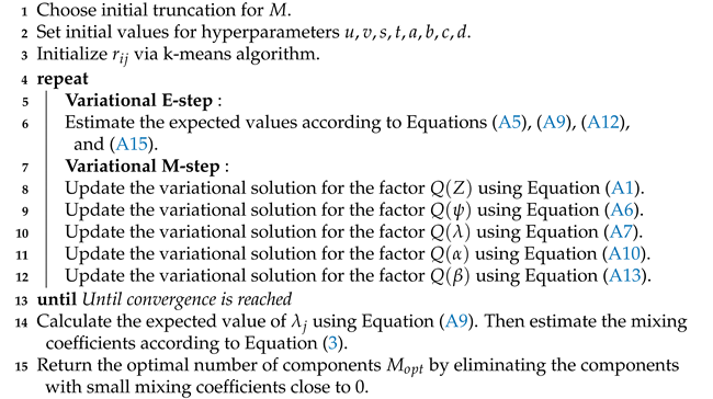
4.2. Learning Algorithm

As explained at the beginning, the objective of this work is to approximate the true posterior $p(\mathrm{\Theta }\mid Y)$ with a new tractable approximation denoted by $Q(\mathrm{\Theta })$. Furthermore, the optimal solution of variational learning is reached while maximizing the lower bound w.r.t $\mathrm{\Theta }=\{Z,\lambda ,\alpha ,\beta \}$. The factorization of $Q(\mathrm{\Theta })$ (while taking into account the truncation M) leads to following parametric form which optimal solution is presented in Appendix A:

$$Q(\mathrm{\Theta })=\left[\prod _{i=1}^N\prod _{j=1}^{M}Q(Z_{ij})\right]\left[\prod _{j=1}^{M}Q({\lambda }_j)Q({\psi }_j)\right]\left[\prod _{j=1}^M\prod _{d=1}^{D}Q({\alpha }_{jd})Q({\beta }_{jd})\right]$$

(17)

Once the optimal variational factors are in hand, the calculation of the lower bound $\mathcal{L}(Q)$ is then straightforward. Figure 2 presents a graphical model of the proposed infinite Gamma mixture model (inGaMM). Random variables are denoted by circles and hyperparameters are represented by rounded boxes. Then, the different steps of the implemented method are summarized in Algorithm 1.

Algorithm 1: Batch variational learning approach for the inGaMM

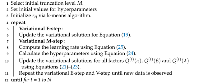
5. Online Variational Bayesian Learning

Early warning and immediate detection of oil spills has many advantages such as immediate response and reducing damage to the environment. The development of real-time monitoring and detection system is of great importance in order to minimize the volume of oil spilled. To address this problem, we propose to develop an online learning approach which is being commonly used in many other areas especially when data points are continuously arriving over time [53]. The online setting is particularly useful for incrementally training the system by feeding instances of data sequentially. It also has the benefit of making the learning process easier and faster than batch mode.

In what follows, we extend the batch variational method (presented in previous section) for unsupervised SAR images classification to an online setting. This process requires updating the model’s parameters incrementally without degrading its efficiency and flexibility. To determine the lower bound, we suppose that we have at time t a fixed set of observed data. At time $t+1$, a new SAR image $Y_{N+1}$ comes out and is added to the dataset, hence, the mixtures’ parameters have to be updated accordingly. Thus, in online setting, the lower bound at time t is expressed as in [54]:

$${\mathcal{L}}^t(Q)=\frac{N}{t}\sum _{i=1}^t\int Q(\mathrm{\Omega })d\mathrm{\Omega }\sum _{Z_i}ln\left[\frac{p(\overrightarrow{Y_i},\overrightarrow{Z_i}\mid \mathrm{\Omega })}{Q(\overrightarrow{Z_i})}\right]+\int Q(\mathrm{\Omega })ln\left[\frac{p(\mathrm{\Omega })}{Q(\mathrm{\Omega })}\right]d\mathrm{\Omega }$$

(18)

where $\mathrm{\Omega }=\{\alpha ,\beta \}$.

Let’s suppose that we already observed $\{\overrightarrow{Y_1},\cdots ,{\overrightarrow{Y}}_{(t-1)}\}$ and then a new data point $\overrightarrow{Y_t}$ is coming. Therefore, ${\mathcal{L}}^t(Q)$ is maximized w.r.t $Q(\overrightarrow{Z_t})$, such that $Q(\alpha )$, $Q(\lambda )$ and $Q(\beta )$ are set to $Q^{t-1}(\alpha )$, $Q^{t-1}(\lambda )$ and $Q^{t-1}(\beta )$, respectively. We adopt a truncation technique with value M which gives [49]:

$$Q(\overrightarrow{Z_t})=\prod _{j=1}^M{r}_{tj}^{Z_{tj}}$$

(19)

$$r_{tj}=\frac{{\rho }_{tj}}{{\sum }_{j=1}^M{\rho }_{tj}}$$

(20)

Then, ${\mathcal{L}}^t(Q)$ is maximized w.r.t $Q(\alpha )$, $Q(\lambda )$ and $Q(\beta )$ while keeping $Q(\overrightarrow{Z_t})$ fixed.

$$Q^{(t)}(\overrightarrow{\alpha })=\prod _{j=1}^M\prod _{d=1}^D\mathcal{G}({\alpha }_{jd}^{(t)}\mid u_{jd}^{*(t)},v_{jd}^{*(t)})$$

(21)

$$Q^{(t)}(\overrightarrow{\beta })=\prod _{j=1}^M\prod _{d=1}^D\mathcal{G}({\beta }_{jd}^{(t)}\mid s_{jd}^{*(t)},t_{jd}^{*(t)})$$

(22)

$$Q^{(t)}(\lambda )=\prod _{j=1}^{M}Beta({\lambda }_j^{(t)}\mid c_j^{(t)},d_j^{(t)})$$

(23)

where

$$\begin{array}{cc}\hfill u_{jd}^{*(t)}& =u_{jd}^{*(t-1)}+{\rho }_t\Delta u_{jd}^{*(t)}\hfill \\ \hfill v_{jd}^{*(t)}& =v_{jd}^{*(t-1)}+{\rho }_t\Delta v_{jd}^{*(t)}\hfill \\ \hfill s_{jd}^{*(t)}& =s_{jd}^{*(t-1)}+{\rho }_t\Delta s_{jd}^{*(t)}\hfill \\ \hfill t_{jd}^{*(t)}& =t_{jd}^{*(t-1)}+{\rho }_t\Delta t_{jd}^{*(t)}\hfill \\ \hfill c_{jd}^{*(t)}& =c_{jd}^{*(t-1)}+{\rho }_t\Delta c_{jd}^{*(t)}\hfill \\ \hfill d_{jd}^{*(t)}& =d_{jd}^{*(t-1)}+{\rho }_t\Delta d_{jd}^{*(t)}\hfill \end{array}$$

(24)

$\Delta$ is the natural gradient of each hyperparameter in the previous equation. ${\rho }_t$ denotes the learning rate [55] expressed by following equation:

$${\rho }_t={({\eta }_0+t)}^{-ϵ}$$

(25)

where $ϵ\in [0.5,1]$ and $\eta \ge 0$. This helps to guarantee convergence [55]. Please note that the expectation in the above mentioned equations are obtained with same manner as for the case of batch setting in the previous section and as in [56]. Since the online learning framework can be considered as a stochastic approximation algorithm, the convergence is ensured as prove in [53]. The proposed and developed online variational algorithm is presented in Algorithm 2.

Algorithm 2: Proposed online algorithm for inGaMM

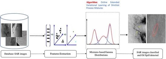
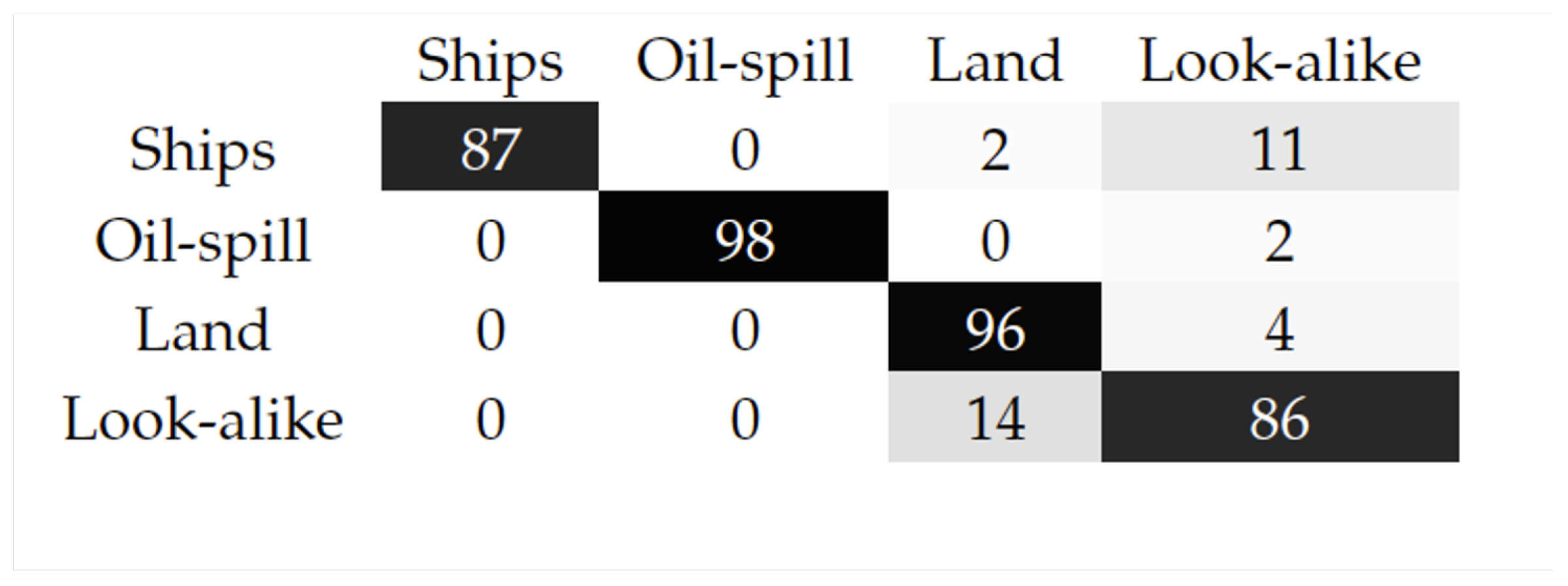
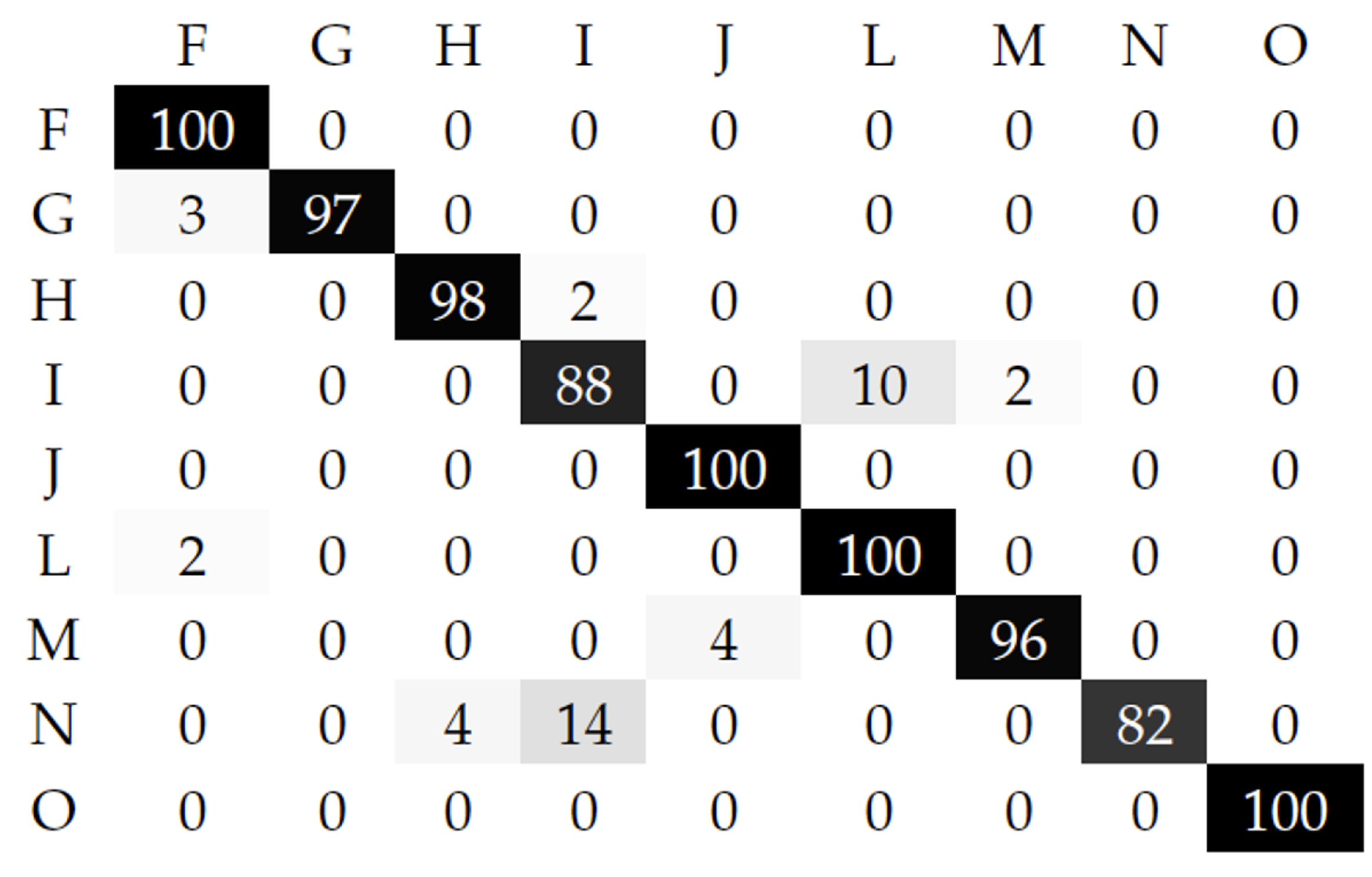
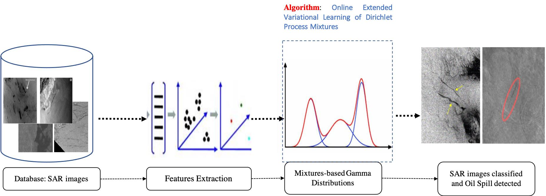
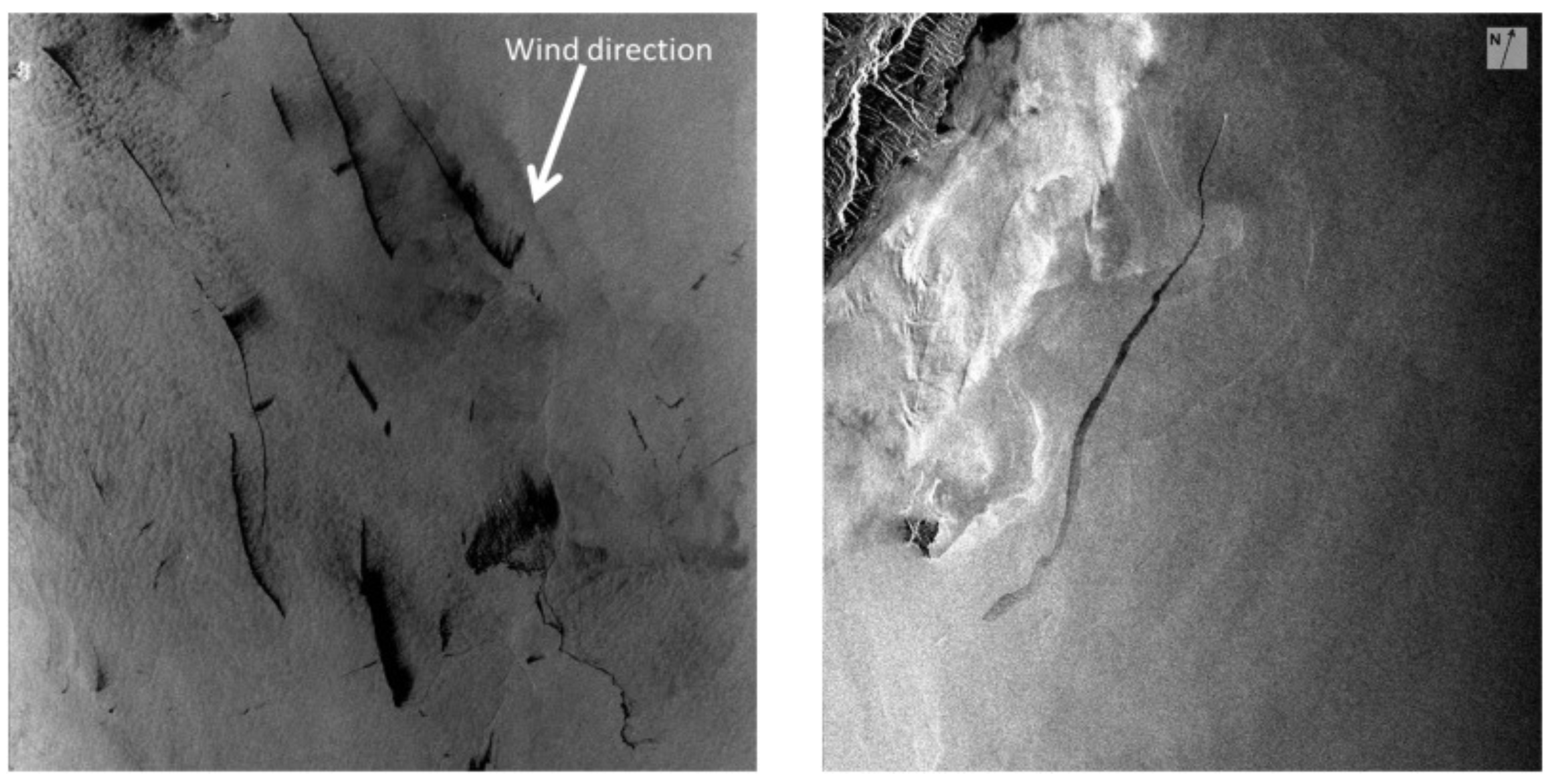
6. Experimental Results

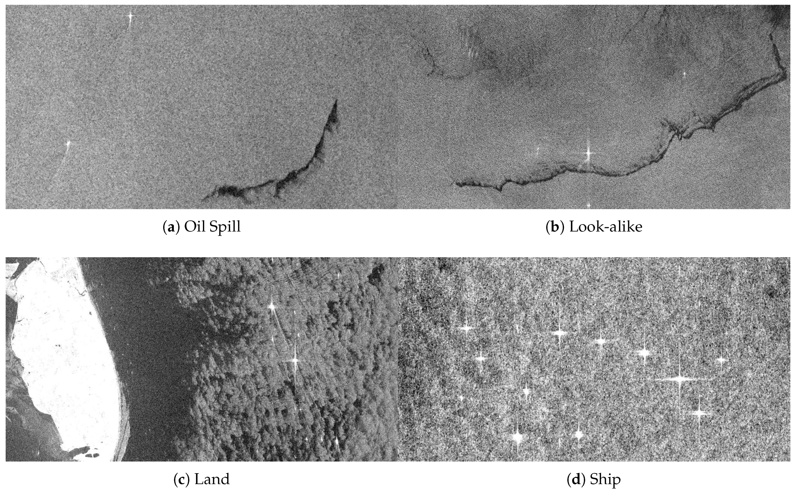
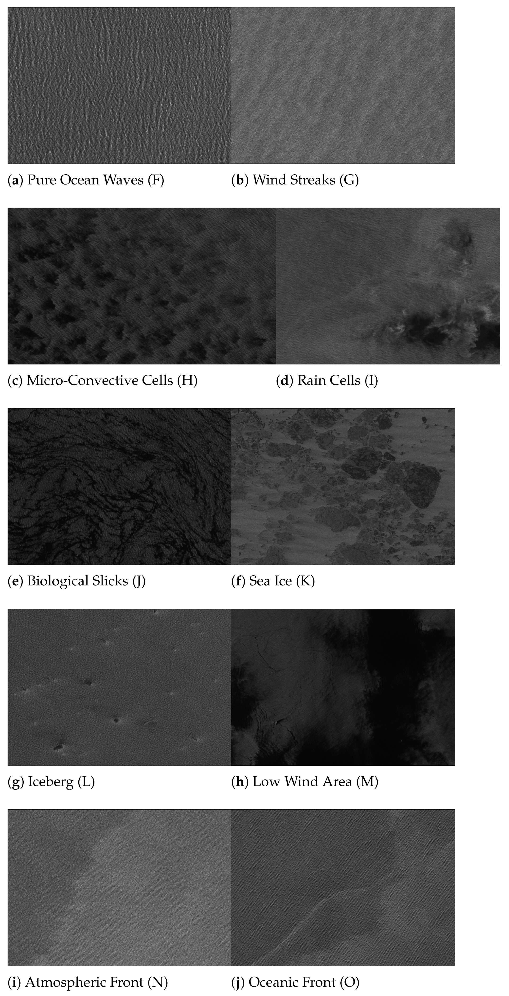
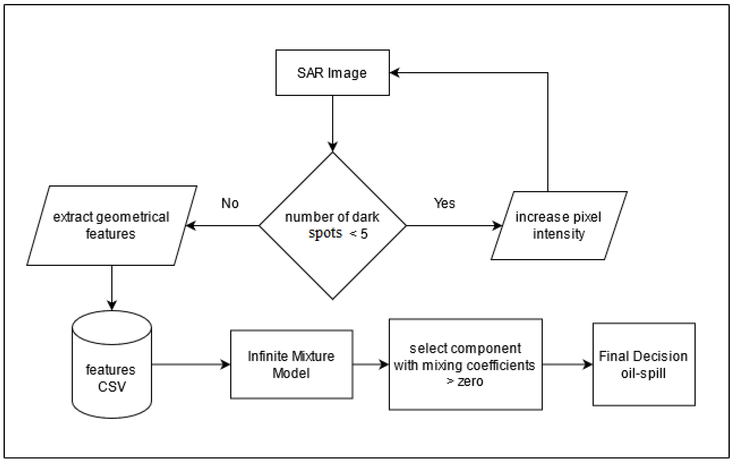
6.1. Data Sets

The main objective of this section is to investigate our developed online extended variational learning framework of Dirichlet process mixture of Gamma distributions to detect oil spills in several SAR images. The second objective is to compare the performance of the proposed statistical framework with other methods from the state-of-art. First, it should be noted that one of the challenges is the lack of already common data sets for oil spill detection and this problem has been addressed by many relevant research communities such as [57,58]. Very limited data sets have been proposed in the literature, and therefore, it is too difficult to compare between published results since each method uses different data sets with different settings. In this work, we are essentially concerned with two challenging SAR databases. The first data set is the SAR images containing oil spills collected via the European Space Agency (ESA) database [40] which is composed of 1112 images with 5 different classes: Land, Look-alike, oil-spill, ships, and sea surface. The second one is a labelled SAR dataset taken from Sentinel-1 wave mode (TenGeoP-SARwv) [59] which includes 40,553 images with 10 different geophysical phenomena such as Pure Ocean Waves (F), Wind Streaks (G), Micro Convective Cells (H), Rain Cells (I), Biological Slicks (J), Sea Ice (K), Iceberg (L), Low Wind Area (M), Atmospheric Front (N), and Oceanic Front (O). Figure 3 and Figure 4 show examples of images from these two datasets, respectively. For experiments, we randomly select half of the dataset as the training set and the rest for testing. In order to quantify how well SAR images are classified, we report the results in terms of average accuracy metric and false positive rate (FPR).

Modeling and classifying SAR requires powerful statistical models to represent their content (ex. color, texture). In this work we shall focus on the problem of SAR images modeling and classification via extracting local features that describe accurately input images. Indeed, feature extraction step is a part of the dimensionality reduction process that has been broadly studied in the past. It has an important role in many computer vision applications since it helps identifying the most discriminating characteristics, reducing ambiguity and enhancing the performance. However, the presence of speckle noise in synthetic aperture radar (SAR) images, as well as low-resolution between regions (surfaces) and poor contrast, make extracting relevant features too difficult. Thus, if the representative features are well extracted, then we can correctly interpret and classify images. Extracting local features from grey-scale images is a well-studied step in the fields of image processing and computer vision and various comparative measures have been studied for many years. The study of prior techniques is not within the scope of this paper. However, we suggest applying two successful methods of features extraction. The first one is based on imageNet pretrained deep learning model (resnet50) [60]. The flowchart diagram for extracting features using resnet50 is given in Figure 5. For each SAR image in the flowchart, we first apply different image processing operations like adjusting contrast value, thresholding, object edge detection by blurring noise and small objects. After this step, based on the number of detected dark spots, we extract different features including geometrical characteristics and texture of the object. Finally, we store the extracted features for the model evaluation. In the second approach, we extract a number of features based on geometrical characteristics, physical behavior, and those related to oil spill context of the dark formations as described in [61]. After extracting features, we applied principal component analysis (PCA) to reduce dimensionality of extracted datasets features.

6.2. Results and Discussion

Next, we apply our online extended variational algorithm (Section 5) over the extracted features. Thus, each image is represented by an infinite Gamma mixture model. We average the results over 30 runs to evaluate and compute the final performance.

Table 1. Results for both dataset with different number of classes using first feature extraction approach (ImageNet pretrained (resnet50) features).

Datasets	No of Class	Accuracy (%)	FPR
ESA-SAR dataset	2	97.96	0.02
ESA-SAR dataset	4	90.57	0.09
Sentinel-1 wave mode SAR dataset	2	94.53	0.05
Sentinel-1 wave mode SAR dataset	9	95.16	0.04

and

Table 2. Results for both dataset with different number of classes using second feature extraction approach (Dark spots, geometrical, physical, and characteristics features).

Datasets	No of Class	Accuracy (%)	FPR
ESA-SAR dataset	2	89.94	0.09
ESA-SAR dataset	4	85.13	0.12
Sentinel-1 wave mode SAR dataset	2	88.68	0.11
Sentinel-1 wave mode SAR dataset	9	82.22	0.14

show the average classification accuracy and false positive rate (FPR) of our InGaMM-eV model. They are obtained with different classes in both datasets and by using two features extraction methods. Indeed, we considered a first experiment where the goal was to distinguish between oil spills versus the rest and a second one where the goal is to categorize some classes from each data set (4 categories are taken from the first data set and 9 from the second one). The testing data is assumed to arrive sequentially in an online mode.

Figure 6 and Figure 7 present the confusion matrices for SAR images classification computed by the proposed InGaMM-eV using the two features extraction methods, respectively. It is noted that these matrices are used to describe the performance of the proposed model since they record true positives, false positives and false negatives. In fact, each matrix summarizes the prediction results on a classification problem and it offers a clear idea of what the proposed model is working correctly and what kinds of errors it commits. Each entry of index $(u,v)$ represents the number of images in class u that are affected to class v. According to these results, the average classification accuracy is very promising and is equal to 90.57% (error rate of 9%) for the first dataset and 95.16% (error rate of 4%) for the second dataset.

Figure 6 and Figure 7 present additional results obtained by changing the way visual features are extracted as well as the number of classes. Indeed, for the case of ESA-SAR dataset, InGaMM-eV provides high average accuracy of 97.96% using imageNet pretrained deep learning model (resnet50), and 89.94% using Dark spots, geometrical, physical characteristics features. In both cases, the false positive rate is very low. For Sentinel-1 wave mode SAR dataset, the average accuracy to classify SAR images is 95.16% using resnet50, which is better than the second method for extracting features (only 88.68%). According to these results, we notice that the overall average classification accuracy is very encouraging, taking into account the complexity of treated images. It is noteworthy that, due to low resolution of images in the second dataset (Sentinel-1 wave mode), it was very difficult to extract features using the second feature extraction method (i.e., detecting dark objects). Thus, we have low accuracy than expected for this dataset.

In this experiment, our second goal is also to demonstrate the advantages of using extended variational framework over the maximum likelihood (via EM-algorithm), as well as the merits of infinite mixture model over its finite counterpart. Therefore, we compared the classification results using the following mixture models: InGaMM-eV (our infinite Gamma model using extended variational inference), GaMM-eV (finite Gamma model using extended variational learning), GaMM-EM (finite Gamma mixture model using expectation maximization learning), InGMM-eV (infinite Gaussian model using extended variational learning), and GMM-EM (finite Gaussian mixture model using expectation maximization learning). The average performances of all tested learning approaches, using the two features extraction methods, are depicted in

Table 3. Overall oil spill detection rate of different models for 2 datasets using the first feature extraction approach (ImageNet pretrained (resnet50) features).

Dataset	InGaMM-eV (Our Approach)	GaMM-eV	GaMM-EM	InGMM-eV	GMM-EM
ESA-SAR	90.05	88.33	86.07	83.21	83.11
Sentinel-1 wave SAR	91.12	89.40	87.02	84.14	83.99

and

Table 4. Overall oil spill detection rate of different models for 2 datasets using the second feature extraction approach (Dark spots, geometrical, physical, and characteristics features).

Dataset	InGaMM-eV (Our Approach)	GaMM-eV	GaMM-EM	InGMM-eV	GMM-EM
ESA-SAR	88.18	87.09	85.11	82.13	82.01
Sentinel-1 wave SAR	89.12	88.11	86.00	83.77	83.07

. We can see clearly that the extended variational approach provides better results than the EM. Furthermore, the merits of using a Dirichlet process mixtures of Gamma distributions (i.e. infinite mixture model ) over a finite mixture model is clear by noting that better result was found with the infinite mixtures. In particular, in Table 3, the InGaMM-eV (90.05%) outperforms GaMM-eV (88.33%) in terms of classification accuracy rate for both datasets. On the other side, it is worth mentioning that our approach provides better results than the implemented frameworks based on Gaussian mixtures. We can then deduce that the infinite Gamma model has better modeling and classification capability than the Gaussian when dealing with SAR images analysis.

Next, The proposed learning approach (InGaMM-eV) is compared with some methods from the literature and the comparative study is presented in

Table 5. Comparative study between different methods from the literature on two datasets.

Method	Dataset	Feature Selection	Accuracy
InGaMM-eV (our approach)	ESA-SAR	ImageNet pretrained (resnet50)	97.96%
InGaMM-eV (our approach)	ESA-SAR	Dark spots, geometrical, physical features	89.94%
Fuzzy classification [62]	ESA-SAR	Georeference, Land masking, and Filtering	88%
InGaMM-eV (our approach)	Sentinel-1 SAR	ImageNet pretrained (resnet50)	94.53%
InGaMM-eV (our approach)	Sentinel-1 SAR	Dark spots, geometrical, physical features	88.68%
Convolutional neural network	Sentinel-1 SAR	Inception v3 CNN	93%
Articial neural network [34]	Sentinel-1 SAR	Dark spot, shape features	87%
Method in [63]	Sentinel-1 SAR	Dark spot features	81%
Method in [64]	Sentinel-1 SAR	Dark spot, shape features	82.61%

. As we can see, the proposed online algorithm performs better than other algorithms. Accordingly, it is important to emphasize the advantage of our developed extended variational formalism for infinite Gamma mixture, which can provide interesting results. It is also important to underline the merit of the online learning process, which is able to maintain high performance of oil spill prediction as well as handling data faster as they arrived. Moreover, it has the capacity to update the model incrementally without the need for retraining. All these results confirm that the proposed infinite Gamma mixture using the extended variational learning mode is a better choice thanks to the flexibility of the infinite Gamma mixture over the finite models. All these benefits make it more appropriate especially for SAR images classification especially in the case or large scale data sets.

7. Conclusions

In this paper an effective online nonparametric Bayesian analysis method based on Dirichlet process mixture of Gamma distributions (i.e., infinite Gamma mixture model) is developed to deal with the challenging problem of oil spill detection in SAR images. The Gamma distribution is considered because of its flexibility for semi-bounded data modelling. This framework is learned using an extended version of conventional variational inference in a flexible way which has certain advantages such as approximating the posteriors effectively in a closed form, easy assessment of convergence and easy optimization by offering a trade-off between frequentist techniques and MCMC-based ones. An important property of our approach is that it does not need the specification of the number of mixture components in advance. The proposed online algorithm has also the benefit to allow data instances to be treated in a sequential manner, which is more attractive than batch learning especially when dealing with massive and streaming data. Through the challenging application of oil spill detection in SAR images, we have demonstrated the performance of our statistical framework, which is able to provide very encouraging results in terms of SAR images modeling and classification capabilities. As future work, we plan to integrate a feature selection mechanism into the proposed framework in order to improve more the classification accuracy. It is our hope that many other real-world applications related to image processing and machine learning can be addressed via our developed framework.

References

1. Lary, D.J.; Alavi, A.H.; Gandomi, A.H.; Walker, A.L. Machine learning in geosciences and remote sensing. Geosci. Front. 2016, 7, 3–10. [Google Scholar] [CrossRef] [Green Version]
2. Lai, Y.; Ping, Y.; He, W.; Wang, B.; Wang, J.; Zhang, X. Variational Bayesian inference for finite inverted Dirichlet mixture model and its application to object detection. Chin. J. Electron. 2018, 27, 603–610. [Google Scholar] [CrossRef]
3. McLachlan, G.J.; Peel, D. Finite Mixture Models; John Wiley & Sons: Hoboken, NJ, USA, 2004. [Google Scholar]
4. Andrews, J.L.; McNicholas, P.D.; Subedi, S. Model-based classification via mixtures of multivariate t-distributions. Comput. Stat. Data Anal. 2011, 55, 520–529. [Google Scholar] [CrossRef]
5. Bouguila, N.; Almakadmeh, K.; Boutemedjet, S. A finite mixture model for simultaneous high-dimensional clustering, localized feature selection and outlier rejection. Expert Syst. Appl. 2012, 39, 6641–6656. [Google Scholar] [CrossRef]
6. Elguebaly, T.; Bouguila, N. Background subtraction using finite mixtures of asymmetric Gaussian distributions and shadow detection. Mach. Vis. Appl. 2014, 25, 1145–1162. [Google Scholar] [CrossRef]
7. Elguebaly, T.; Bouguila, N. Bayesian Learning of Generalized Gaussian Mixture Models on Biomedical Images. In Artificial Neural Networks in Pattern Recognition, Proceedings of the 4th IAPR TC3 Workshop, ANNPR 2010, Cairo, Egypt, 11–13 April 2010; Schwenker, F., Gayar, N.E., Eds.; Springer: Berlin, Germany, 2010; Volume 5998, pp. 207–218. [Google Scholar] [CrossRef] [Green Version]
8. Lai, Y.; Cao, H.; Luo, L.; Zhang, Y.; Bi, F.; Gui, X.; Ping, Y. Extended variational inference for gamma mixture model in positive vectors modeling. Neurocomputing 2021, 432, 145–158. [Google Scholar] [CrossRef]
9. Li, H.; Krylov, V.A.; Fan, P.; Zerubia, J.; Emery, W.J. Unsupervised Learning of Generalized Gamma Mixture Model with Application in Statistical Modeling of High-Resolution SAR Images. IEEE Trans. Geosci. Remote Sens. 2016, 54, 2153–2170. [Google Scholar] [CrossRef] [Green Version]
10. Ziou, D.; Bouguila, N. Unsupervised Learning of a Finite Gamma Mixture Using MML: Application to SAR Image Analysis. In Proceedings of the 17th International Conference on Pattern Recognition, (ICPR 2004), Cambridge, UK, 23–26 August 2004; pp. 68–71. [Google Scholar] [CrossRef]
11. Al-Osaimi, F.R.; Bouguila, N. A Finite Gamma Mixture Model-Based Discriminative Learning Frameworks. In Proceedings of the 14th IEEE International Conference on Machine Learning and Applications, ICMLA 2015, Miami, FL, USA, 9–11 December 2015; Li, T., Kurgan, L.A., Palade, V., Goebel, R., Holzinger, A., Verspoor, K., Wani, M.A., Eds.; IEEE: New York, NY, USA, 2015; pp. 819–824. [Google Scholar] [CrossRef]
12. Beckmann, C.; Woolrich, M.; Smith, S. Gaussian/Gamma mixture modelling of ICA/GLM spatial maps. In Proceedings of the 9th International Conference on Functional Mapping of the Human Brain, New York, NY, USA, 19–22 June 2003. [Google Scholar]
13. Alharithi, F.S.; Almulihi, A.H.; Bourouis, S.; Alroobaea, R.; Bouguila, N. Discriminative Learning Approach Based on Flexible Mixture Model for Medical Data Categorization and Recognition. Sensors 2021, 21, 2450. [Google Scholar] [CrossRef]
14. Bourouis, S.; Channoufi, I.; Alroobaea, R.; Rubaiee, S.; Andejany, M.; Bouguila, N. Color object segmentation and tracking using flexible statistical model and level-set. Multim. Tools Appl. 2021, 80, 5809–5831. [Google Scholar] [CrossRef]
15. Fan, W.; Bouguila, N.; Bourouis, S.; Laalaoui, Y. Entropy-based variational Bayes learning framework for data clustering. IET Image Process. 2018, 12, 1762–1772. [Google Scholar] [CrossRef]
16. Najar, F.; Bourouis, S.; Zaguia, A.; Bouguila, N.; Belghith, S. Unsupervised Human Action Categorization Using a Riemannian Averaged Fixed-Point Learning of Multivariate GGMM. In Proceedings of the Image Analysis and Recognition—15th International Conference, ICIAR 2018, Póvoa de Varzim, Portugal, 27–29 June 2018; pp. 408–415. [Google Scholar]
17. Ferguson, T.S. Bayesian density estimation by mixtures of normal distributions. In Recent Advances in Statistics; Academic Press: New York, NY, USA, 1983; pp. 287–302. [Google Scholar]
18. Rasmussen, C.E. A Practical Monte Carlo Implementation of Bayesian Learning. In Proceedings of the Advances in Neural Information Processing Systems 8, NIPS, Denver, CO, USA, 27–30 November 1995; Touretzky, D.S., Mozer, M., Hasselmo, M.E., Eds.; MIT Press: Cambridge, MA, USA, 1995; pp. 598–604. [Google Scholar]
19. Bourouis, S.; Alroobaea, R.; Rubaiee, S.; Andejany, M.; Almansour, F.M.; Bouguila, N. Markov Chain Monte Carlo-Based Bayesian Inference for Learning Finite and Infinite Inverted Beta-Liouville Mixture Models. IEEE Access 2021, 9, 71170–71183. [Google Scholar] [CrossRef]
20. Bouguila, N.; Elguebaly, T. A fully Bayesian model based on reversible jump MCMC and finite Beta mixtures for clustering. Expert Syst. Appl. 2012, 39, 5946–5959. [Google Scholar] [CrossRef]
21. Jordan, M.I.; Ghahramani, Z.; Jaakkola, T.S.; Saul, L.K. An Introduction to Variational Methods for Graphical Models. Mach. Learn. 1999, 37, 183–233. [Google Scholar] [CrossRef]
22. Fan, W.; Bouguila, N. Online Learning of a Dirichlet Process Mixture of Beta-Liouville Distributions Via Variational Inference. IEEE Trans. Neural Netw. Learn. Syst. 2013, 24, 1850–1862. [Google Scholar] [CrossRef] [PubMed]
23. Elguebaly, T.; Bouguila, N. A Bayesian approach for SAR images segmentation and changes detection. In Proceedings of the 2010 25th Biennial Symposium on Communications, Kingston, ON, Canada, 12–14 May 2010; pp. 24–27. [Google Scholar] [CrossRef]
24. Zhao, J.; Temimi, M.; Ghedira, H.; Hu, C. Exploring the potential of optical remote sensing for oil spill detection in shallow coastal waters-a case study in the Arabian Gulf. Opt. Express 2014, 22, 13755–13772. [Google Scholar] [CrossRef]
25. Singha, S.; Bellerby, T.J.; Trieschmann, O. Detection and classification of oil spill and look-alike spots from SAR imagery using an Artificial Neural Network. In Proceedings of the 2012 IEEE International Geoscience and Remote Sensing Symposium, IGARSS 2012, Munich, Germany, 22–27 July 2012; pp. 5630–5633. [Google Scholar]
26. Brekke, C.; Solberg, A.H. Oil spill detection by satellite remote sensing. Remote Sens. Environ. 2005, 95, 1–13. [Google Scholar] [CrossRef]
27. Salberg, A.; Larsen, S.O. Classification of Ocean Surface Slicks in Simulated Hybrid-Polarimetric SAR Data. IEEE Trans. Geosci. Remote Sens. 2018, 56, 7062–7073. [Google Scholar] [CrossRef]
28. Alpers, W.; Holt, B.; Zeng, K. Oil spill detection by imaging radars: Challenges and pitfalls. Remote Sens. Environ. 2017, 201, 133–147. [Google Scholar] [CrossRef]
29. Solberg, A.H.S.; Storvik, G.; Solberg, R.; Volden, E. Automatic detection of oil spills in ERS SAR images. IEEE Trans. Geosci. Remote Sens. 1999, 37, 1916–1924. [Google Scholar] [CrossRef] [Green Version]
30. Skrunes, S.; Brekke, C.; Eltoft, T. Characterization of Marine Surface Slicks by Radarsat-2 Multipolarization Features. IEEE Trans. Geosci. Remote Sens. 2014, 52, 5302–5319. [Google Scholar] [CrossRef] [Green Version]
31. Fingas, M.; Brown, C.E. A Review of Oil Spill Remote Sensing. Sensors 2018, 18, 91. [Google Scholar] [CrossRef] [Green Version]
32. Fiscella, B.; Giancaspro, A.; Nirchio, F.; Pavese, P.; Trivero, P. Oil spill detection using marine SAR images. Int. J. Remote Sens. 2000, 21, 3561–3566. [Google Scholar] [CrossRef]
33. Gambardella, A.; Giacinto, G.; Migliaccio, M.; Montali, A. One-class classification for oil spill detection. Pattern Anal. Appl. 2010, 13, 349–366. [Google Scholar] [CrossRef]
34. Topouzelis, K.; Karathanassi, V.; Pavlakis, P.; Rokos, D. Detection and discrimination between oil spills and look-alike phenomena through neural networks. ISPRS J. Photogramm. Remote Sens. 2007, 62, 264–270. [Google Scholar] [CrossRef]
35. Karantzalos, K.; Argialas, D. Automatic detection and tracking of oil spills in SAR imagery with level set segmentation. Int. J. Remote Sens. 2008, 29, 6281–6296. [Google Scholar] [CrossRef]
36. Chang, L.; Tang, Z.S.; Chang, S.H.; Chang, Y. A region-based GLRT detection of oil spills in SAR images. Pattern Recognit. Lett. 2008, 29, 1915–1923. [Google Scholar] [CrossRef]
37. Solberg, A.H.S.; Brekke, C.; Husoy, P.O. Oil Spill Detection in Radarsat and Envisat SAR Images. IEEE Trans. Geosci. Remote Sens. 2007, 45, 746–755. [Google Scholar] [CrossRef]
38. Keramitsoglou, I.; Cartalis, C.; Kiranoudis, C.T. Automatic identification of oil spills on satellite images. Environ. Model. Softw. 2006, 21, 640–652. [Google Scholar] [CrossRef]
39. Cantorna, D.; Dafonte, C.; Iglesias, A.; Varela, B.A. Oil spill segmentation in SAR images using convolutional neural networks. A comparative analysis with clustering and logistic regression algorithms. Appl. Soft Comput. 2019, 84, 105716. [Google Scholar] [CrossRef]
40. Krestenitis, M.; Orfanidis, G.; Ioannidis, K.; Avgerinakis, K.; Vrochidis, S.; Kompatsiaris, I. Oil Spill Identification from Satellite Images Using Deep Neural Networks. Remote Sens. 2019, 11, 1762. [Google Scholar] [CrossRef] [Green Version]
41. Orfanidis, G.; Ioannidis, K.; Avgerinakis, K.; Vrochidis, S.; Kompatsiaris, I. A Deep Neural Network for Oil Spill Semantic Segmentation in Sar Images. In Proceedings of the 2018 IEEE International Conference on Image Processing, ICIP 2018, Athens, Greece, 7–10 October 2018; pp. 3773–3777. [Google Scholar]
42. Song, D.; Ding, Y.; Li, X.; Zhang, B.; Xu, M. Ocean Oil Spill Classification with RADARSAT-2 SAR Based on an Optimized Wavelet Neural Network. Remote Sens. 2017, 9, 799. [Google Scholar] [CrossRef] [Green Version]
43. Li, J.; Du, Q.; Li, Y. An efficient radial basis function neural network for hyperspectral remote sensing image classification. Soft Comput. 2016, 20, 4753–4759. [Google Scholar] [CrossRef]
44. Shaban, M.; Salim, R.; Abu Khalifeh, H.; Khelifi, A.; Shalaby, A.; El-Mashad, S.; Mahmoud, A.; Ghazal, M.; El-Baz, A. A Deep-Learning Framework for the Detection of Oil Spills from SAR Data. Sensors 2021, 21, 2351. [Google Scholar] [CrossRef]
45. Zeng, K.; Wang, Y. A Deep Convolutional Neural Network for Oil Spill Detection from Spaceborne SAR Images. Remote Sens. 2020, 12, 1015. [Google Scholar] [CrossRef] [Green Version]
46. Topouzelis, K.N. Oil Spill Detection by SAR Images: Dark Formation Detection, Feature Extraction and Classification Algorithms. Sensors 2008, 8, 6642–6659. [Google Scholar] [CrossRef] [Green Version]
47. Teh, Y.W. Dirichlet Process. In Encyclopedia of Machine Learning; Sammut, C., Webb, G.I., Eds.; Springer: Boston, MA, USA, 2010; pp. 280–287. [Google Scholar]
48. Sethuraman, J. A constructive definition of Dirichlet priors. Stat. Sin. 1994, 4, 639–650. [Google Scholar]
49. Blei, D.M.; Jordan, M.I. Variational inference for Dirichlet process mixtures. Bayesian Anal. 2006, 1, 121–143. [Google Scholar] [CrossRef]
50. Ishwaran, H.; James, L.F. Gibbs sampling methods for stick-breaking priors. J. Am. Stat. Assoc. 2001, 96, 161–173. [Google Scholar] [CrossRef]
51. Opper, M.; Saad, D. Advanced Mean Field Methods: Theory and Practice; MIT Press: Cambridge, MA, USA, 2001. [Google Scholar]
52. Blei, D.M.; Jordan, M.I. Variational methods for the Dirichlet process. In Machine Learning, Proceedings of the Twenty-First International Conference (ICML 2004), Banff, AL, Canada, 4–8 July 2004; Brodley, C.E., Ed.; ACM International Conference Proceeding Series; ACM: New York, NY, USA, 2004; Volume 69. [Google Scholar]
53. Sato, M. Online Model Selection Based on the Variational Bayes. Neural Comput. 2001, 13, 1649–1681. [Google Scholar] [CrossRef]
54. Fan, W.; Bouguila, N. Online variational learning of generalized Dirichlet mixture models with feature selection. Neurocomputing 2014, 126, 166–179. [Google Scholar] [CrossRef]
55. Hoffman, M.D.; Blei, D.M.; Bach, F.R. Online Learning for Latent Dirichlet Allocation. In Advances in Neural Information Processing Systems; Curran Associates, Inc.: New York, NY, USA, 2010; pp. 856–864. [Google Scholar]
56. Manouchehri, N.; Nguyen, H.; Koochemeshkian, P.; Bouguila, N.; Fan, W. Online Variational Learning of Dirichlet Process Mixtures of Scaled Dirichlet Distributions. Inf. Syst. Front. 2020, 22, 1085–1093. [Google Scholar] [CrossRef]
57. Konik, M.; Bradtke, K. Object-oriented approach to oil spill detection using ENVISAT ASAR images. ISPRS J. Photogramm. Remote Sens. 2016, 118, 37–52. [Google Scholar] [CrossRef]
58. Topouzelis, K.; Psyllos, A. Oil spill feature selection and classification using decision tree forest on SAR image data. ISPRS J. Photogramm. Remote Sens. 2012, 68, 135–143. [Google Scholar] [CrossRef]
59. Wang, C.; Mouche, A.; Tandeo, P.; Stopa, J.E.; Longépé, N.; Erhard, G.; Foster, R.C.; Vandemark, D.; Chapron, B. A labelled ocean SAR imagery dataset of ten geophysical phenomena from Sentinel-1 wave mode. Geosci. Data J. 2019, 6, 105–115. [Google Scholar] [CrossRef] [Green Version]
60. He, K.; Zhang, X.; Ren, S.; Sun, J. Deep Residual Learning for Image Recognition. In Proceedings of the 2016 IEEE Conference on Computer Vision and Pattern Recognition, CVPR 2016, Las Vegas, NV, USA, 27–30 June 2016; IEEE Computer Society: Washington, DC, USA, 2016; pp. 770–778. [Google Scholar]
61. Topouzelis, K.; Stathakis, D.; Karathanassi, V. Investigation of genetic algorithms contribution to feature selection for oil spill detection. Int. J. Remote Sens. 2009, 30, 611–625. [Google Scholar] [CrossRef]
62. Ferraro, G.; Pavlakis, P.; Tarchi, D.; Sieber, A.; Ferraro, G.; Vincent, G. On the Monitoring of Illicit Discharges—A Reconnaissance Study in the Mediterranean Sea; EUR 19906 EN; European Commission: Brussels, Belgium, 2001.
63. Chatziantoniou, A.; Karagaitanakis, A.; Bakopoulos, V.; Papandroulakis, N.; Topouzelis, K. Detection of Biogenic Oil Films near Aquaculture Sites Using Sentinel-1 and Sentinel-2 Satellite Images. Remote Sens. 2021, 13, 1737. [Google Scholar] [CrossRef]
64. Chatziantoniou, A.; Bakopoulos, V.; Papandroulakis, N.; Topouzelis, K. Detection of biogenic oil film near aquaculture sites seen by Sentinel-2 multispectral images. In Remote Sensing of the Ocean, Sea Ice, Coastal Waters, and Large Water Regions 2020; International Society for Optics and Photonics: San Diego, CA, USA, 2020; p. 4. [Google Scholar] [CrossRef]
Figure 1. SAR image obtained by the European Remote Sensing satellite ERS-2 on April 1997 over the South China Sea (left image) and SAR image obtained by the ERS-1 satellite on May 1994 over Pacific Ocean east of Taiwan (right image). These images (area: 100 km × 100 km) showing an oil spill [28].
Remotesensing 13 02991 g001
Figure 2. Graphical model of the developed variational infinite inGaMM. Random variables are denoted by circles and hyperparameters are represented by rounded boxes. Y is observed variable, Z is latent variable, large boxes are used for repeated process and the arrows show the conditional dependence between variables.
Remotesensing 13 02991 g002
Figure 3. Dataset-1: Samples of SAR images from the European Space Agency (ESA) dataset [40]. (a) OilSpill, (b) Look-alike, (c) Land, (d) Ship.
Remotesensing 13 02991 g003
Figure 4. Dataset-2: Samples of SAR images from Sentinel-1 wave mode (TenGeoP-SARwv) dataset [59]. (a) Pure Ocean Waves, (b) Wind Streaks, (c) Micro-Convective Cells, (d) Rain Cells, (e) Biological Slicks, (f) Sea Ice, (g) Iceberg, (h) Low Wind Area, (i) Atmospheric Front, (j) Oceanic Front.
Remotesensing 13 02991 g004
Figure 5. Flowchart diagram for extracting features using first feature extraction approach (ImageNet pretrained (resnet50) features).
Remotesensing 13 02991 g005
Figure 6. Average rounded confusion matrix (in terms of percentage) for SAR classification using InGaMM-eV for ESA-SAR dataset.
Remotesensing 13 02991 g006
Figure 7. Average rounded confusion matrix (in terms of percentage) for SAR classification using InGaMM-eV for Sentinel-1 wave mode SAR dataset.
Remotesensing 13 02991 g007