Article

Mapping Maize Area in Heterogeneous Agricultural Landscape with Multi-Temporal Sentinel-1 and Sentinel-2 Images Based on Random Forest

1
Key Laboratory of Remote Sensing of Gansu Province, Heihe Remote Sensing Experimental Research Station, Northwest Institute of Eco-Environment and Resources, Chinese Academy of Sciences, Lanzhou 730000, China
2
University of Chinese Academy of Sciences, Beijing 100049, China
*
Author to whom correspondence should be addressed.
Remote Sens. 2021, 13(15), 2988; https://doi.org/10.3390/rs13152988
Submission received: 22 June 2021 / Revised: 26 July 2021 / Accepted: 27 July 2021 / Published: 29 July 2021
(This article belongs to the Special Issue Advances in Remote Sensing for Crop Monitoring and Yield Estimation)

Abstract

:
Accurate estimation of crop area is essential to adjusting the regional crop planting structure and the rational planning of water resources. However, it is quite challenging to map crops accurately by high-resolution remote sensing images because of the ecological gradient and ecological convergence between crops and non-crops. The purpose of this study is to explore the combining application of high-resolution multi-temporal Sentinel-1 (S1) radar backscatter and Sentinel-2 (S2) optical reflectance images for maize mapping in highly complex and heterogeneous landscapes in the middle reaches of Heihe River, northwest China. We proposed a new two-step method of vegetation extraction and followed by maize extraction, that is, extract the vegetation-covered areas first to reduce the inter-class variance by using a Random Forest (RF) classifier based on S2 data, and then extract the maize distribution in the vegetation area by using another RF classifier based on S1 and/or S2 data. The results demonstrate that the vegetation extraction classifier successfully identified vegetation-covered regions with an overall accuracy above 96% in the study area, and the accuracy of the maize extraction classifier constructed by the combined multi-temporal S1 and S2 images is significantly improved compared with that S1 (alone) or S2 (alone), with an overall accuracy of 87.63%, F1_Score of 0.86, and Kappa coefficient of 0.75. In addition, with the introduction of multi-temporal S1 and/or S2 images in crop growing season, the constructed RF model is more beneficial to maize mapping.

1. Introduction

Accurately estimating the spatial distribution and planting area of agricultural objects is of great significance for adjusting crop planting structure and water and soil resource management. Satellite remote sensing (RS) has the unique ability of large-area observation, and great achievements have been made in crop mapping by RS. It has become a common way to obtain large-scale crop planting area information by using RS satellites, such as Landsat satellite, Terra and Aqua satellite, Gaofen-1 satellite, and Sentinel satellite [1,2], with the availability of a series of remote sensing cloud computing platforms, such as google earth engine and Amazon web services. Limited by the spatial and temporal resolution of high-resolution images and the processing ability of massive remote sensing images, low and moderate spatial resolution RS images [3], such as MODIS, AVHRR images, are dominant data sources in the previous study of crop classification and extraction, since these low and moderate remote sensing images hold considerable promise for large area crops mapping given their global coverage, daily temporal resolution, and free access. These low and moderate RS images are beneficial to preliminary understanding of the spatial distribution of crops. However, limited by the coarse spatial resolution of the RS image, it is unable to meet the need of fine mapping requirements of small farmland [4]. Sentinel-2 (S2) is a European wide-format, high-resolution, multi-spectral imaging mission, including two polarities-orbiting satellites S2A and S2B, in the same orbit. The two satellites are complementary, with a wide cover (290 km), moderate revisit period (5 days) and high spatial resolution. It can support the monitoring of vegetation growth season changes [5], significantly reducing the problem of mixed pixels.
Nevertheless, optical RS images are inevitably affected by cloud cover, resulting in the lack of information in space and time, which greatly limits the accuracy of crop mapping. With the outstanding advantage of not being affected by clouds of Synthetic Aperture Radar (SAR) and the strong sensitivity of C-band backscattering signals to crop phenological cycles, SAR images have also been used to monitor the crop distribution extent, plant pattern and growth stage, and achieved high accuracy [6,7]. Sentinel-1 (S1) SAR images with a relatively short revisit time (i.e., 6 days) and high spatial resolution, which can be used to accurately track the crop growth and extract the phenological phase [8]. Previous studies have confirmed the great potential of S1 SAR for crop classification in areas with widespread cloudiness [9]. In addition, recent studies have indicated that the SAR data can replace optical images with the same resolution in the cloudy region [10], and improve the identification of certain crops [11]. Therefore, the potential of combining optical and SAR images to improve the mapping accuracy of crops in highly heterogeneous areas is a topic worth exploring [12].
One of the key points of high-precision crop mapping by using optical RS images is to select the appropriate spectral index. So far, a large number of spectral indices have been constructed for vegetation growth monitoring. Among them, the red edge point (REP) is very sensitive to the change of chlorophyll concentration [13] and the red edge inflection point (REIP) has been used to indicate vegetation stress and senescence [14]. Normalized difference vegetation index (NDVI) quantifies photosynthetic capacity, water stress and vegetation productivity [15]. Meanwhile, the time series of NDVI can be used to observe phenological information of different land cover types [16] and vegetation characteristics [17]. However, NDVI is prone to saturation in areas with high vegetation coverage. Enhanced vegetation index (EVI) has tried to compensate for this by using more spectral information, which further enhances the high vegetation regional sensitivity and reduces the disturbance of the soil and atmosphere [18]. Furthermore, crop growth is also affected by human activities, such as irrigation and fertilization. Normalized difference water index (NDWI) and Land Surface Water Index (LSWI) are two vegetation indices sensitive to surface moisture content [19]. The spatial distribution of green chlorophyll vegetation index (GCVI) is of great significance to the response of fertilizer (nitrogen) [20]. In addition, soil tillage index (STI) and Normalized difference tillage index (NDTI) are useful indices for identifying cultivated land [21]. Crop Residue Cover (CRC) is a vegetation index indicating the density of straw mulch in the field. The normalized burn ratio (NBR) has been used to estimate fire severity [22]. The Normalized difference building index (NDBI) index is also used to discriminate built up areas [23]. For more information on the construction of vegetation indices based on optical RS images, please refer to [24]. In view of the problem of crop mapping in areas with highly complex and heterogeneous vegetation structures, it is almost impossible to distinguish complex variation relationships among different vegetation types only by using single or a few vegetation feature variables. In contrast, if too many vegetation feature variables are used, it will easily lead to information redundancy and a large amount of computation, which can reduce the crop mapping accuracy [25].
Despite the above obstacle, the optimal feature variable combination analysis is used to effectively improve the classification accuracy and reducing data redundancy and time consumption in crop mapping research [26]. It has become a hot topic to search for optimal features from a large number of variables through a special feature selection [27]. At present, many feature selection methods have been developed in crop mapping research, such as stepwise discriminant analysis method [28], Jeffries-Matusita distance [29], separability analysis method [12], mutual information rate [25], the feature selection method based on the variable importance of random forest algorithm [11,30]. In addition, the combination of the above methods has also been proposed to strike a balance between separability and relevance, such as the spectrum-dimensional optimization algorithm [31], the automatic spectral-temporal feature selection method [32], and the combined method of time series correlation analysis, random forest feature importance, and univariate statistical tests with mutual information criteria to select features [33].
In recent years, using machine learning methods to extract crop spatial distribution information has become a research hotspot. The pixel-by-pixel supervised learning algorithm, based on decision tree (DT), maximum likelihood classification (MLC), artificial neural network (ANN), support vector machine (SVM) and random forest (RF), were the most widely used methods for crop spatial distribution information extraction, e.g., Basukala et al., (2007) compared MLC, SVM and RF methods to classify cotton, wheat and rice in the Khorezm Region of Uzbekistan and southern part of Autonomous Republic of Karakalpakstan, the results indicate that the RF performed much better than MLC and SVM, especially for the cases when the number of training samples is limited [34]. Moumni et al., (2021) used three machine learning classifier algorithms, ANN, SVM, and MLC, to map the crop types in irrigated perimeter, their results show that combined images acquired in C-band and the optical range improved clearly the crop types classification performance compared to the classification results of optical or SAR data alone [35]. Peña et al. (2014) evaluated the C4.5 DT, logistic regression (LR), ANN, and SVM, both as single classifiers and combined in a hierarchical classification, for the mapping of nine major summer crops from ASTER satellite images [36]. Zhang et al. (2020) compared the classification and regression tree (CART) DT, SVM, and RF, to map different crop types by using time-series S2 images, and they also further analyzed the effectiveness of the temporal and spectral features [37]. By using ANN, SVM and RF methods, multiple crop types classification was performed by using single Landsat 8, S1, and S2 image, and combined S1, S2, and Landsat 8 images [38]. These studies demonstrate that the RF algorithm achieves relatively higher accuracy in crop types extraction, compared with other machine learning algorithms. The RF method can not only easily handle different data types, but also quantitatively calculate the importance of variables. Meanwhile, unsupervised classification algorithms based on k-means clustering and iterative self-organized class (ISOCLASS) cluster algorithm also have certain advantages when there is no crop label sample [39,40]. However, Biggs et al. (2007) mapped rainfed and irrigated crops using this ISOCLASS cluster algorithm with MODIS NDVI time series images over Krishna Basin, India, and they found the classification accuracy of this method is disappointing in heterogeneous landscapes [41]. In addition, Wardlow and Egbert (2008) proposed a hierarchical classification scheme of combining supervised and unsupervised classification to extract the spatial distribution information of crops in the US Central Great Plains [42], the unsupervised classification method (ISODATA) was applied first to produce the crop/non-crop map, then the supervised decision tree algorithm was applied to produce the three crop maps, and the high classification accuracy (>84%) was attained by this method. Therefore, with enough label samples, supervised learning may be a more direct and effective way to identify the detailed distribution information of crops.
Our goal in this study is to explore more accurate crop classification under complex and heterogeneous vegetation landscapes by combining high-resolution multi-temporal optical and radar images based on RF algorithm. Specifically, a two-step method is proposed in this study, the first step is to extract vegetation cover information based on S2 images, and the second step is to extract maize coverage by using S1 (alone), S2 (alone) and combined data of S1 and S2. Numerous feature variables that may be beneficial to maize classification have been pre-selected in advance. A feature selection process through quantitatively evaluating the importance of the variables based on RF has been implemented to find the best combination of feature variables in the proposed two-step crop mapping. Finally, the accuracy of classifiers for S1 (alone), S2 (alone) and combined data are assessed using the ground reference dataset.
The following section describes the study area and data used in this study and the pre-processing of RS data. Section 3 describes the detailed methodology of maize extraction. Section 4 shows the vegetation extraction results based on S2 and maize extraction results based on S1 (alone), S2 (alone) and combined data, respectively. Section 5 discusses the influence of image pre-processing and multi-temporal images on crop mapping and the advantages of the feature selection program in classification applications. Section 6 is the conclusion of the study.

2. Study Area and Data

2.1. Study Area

The study area is located in the middle reaches of the Heihe River basin, which is the central part of the Hexi Corridor Plain in central Gansu Province, China (Figure 1) [43]. It is a national demonstration area of modern agriculture and the largest corn seed production area in China with flat terrain, fertile soil, sufficient sunshine and convenient water diversion [44]. The climate in this region is arid, with little precipitation but high evapotranspiration [45]. Therefore, the oasis in the study area is dominated by artificial oasis, and the planting structure of crops is highly heterogeneous and diverse [46]. Some areas have realized modern agricultural management, while other areas are small-scale agriculture with landscape fragmentation structure. Crops are primarily one-season planting in this area, and the growth period is mainly from April to September. The crop types in the study area include food crops (i.e., wheat, rice, maize, millet, soybeans and potatoes), cash crops (i.e., cotton, oilseed, hemp, beets, medicinal herbs, vegetables and melons) and green fodder (hybrid seed maize production). Maize is the crop with the largest planting area in this region, with large water requirements and high evapotranspiration during the growth period [47].

2.2. RS Images and Processing

2.2.1. Sentinel-1 Images

S1 level-1 Ground Range Detected (GRD) products are generated by C-band SAR to detect targets in the interferometric wide swath mode for both VV and VH polarizations with 10 m × 10 m pixel size and a swath width of 290 km. The GRD images have been pre-processed into an analysis-ready format using border noise removal, thermal noise removal, radiometric calibration, and orthorectification. As speckle noises impaired the performance of S1 on crop identification [48], further pre-processing included spatial filtering using a 7 × 7 Refined Lee speckle filter for both VV and VH polarizations [49,50]. Two additional indicators (Note, we also regard them as two bands in the rest of the paper), the difference between VV and VH (VV-VH) and the ratio of VV and VH (VV/VH), were also calculated [51].
We collected 67 S1 images with four bands (VV, VH, VV-VH, VV/VH) (Table 1) from a full growing season (i.e., April 1 to September 30) in 2019. As the temporal composite with regular time intervals can overcome the spatial heterogeneity of observations, the monthly median composition method is used to construct S1 data aggregation on a monthly scale [52].

2.2.2. Sentinel-2 Images

The corresponding S2 multi-spectral instrument (MSI) Level-1C (L1C) top-of-atmosphere (TOA) reflectance products, which have been radiated and geometrically corrected [53], are used in this study. A total of 428 images are collected. The pre-processing process of S2 images mainly includes re-projection, resampling, cloud mask and moving median composition. First, re-project the image dataset to the WGS 1984 projected coordinate system. Second, all the bands with the lower spatial resolution are resampled to 10 m with cubic convolution interpolation. Then, the QA60 band is used to evaluate the quality of images and automatically hide the cloud and cirrus pixels in each image [25]. Furthermore, the monthly median composition method is also used for constructing S2 data aggregation on a monthly scale. Finally, the moving median synthesis method is used to smooth and gap-fill the image dataset [52].
In addition to the above four bands, a set of spectral indicators used in many previous studies to indicate vegetation growth have also been calculated. A summary of these spectral indices and their definitions are described in Table 1. In addition to the 11 spectral indices mentioned in Section 1, NBR1 and NBR2 are evolved from the NBR index, and there are four indices, RDNDVI1, RDNDVI2, RDGCVI1 and RDGCVI2, which are respectively extended from NDVI and GCVI indices.

2.3. Ground-Based Reference Dataset

A ground-based reference dataset is collected for model construction and accuracy evaluation. This ground-based reference dataset covers the typical land cover types in the study area, which is a point dataset with spatial and attributes information. A total of 2896 ground-based reference sample points were collected, including 623 maize samples, 731 non-maize vegetation samples, and 1542 non-vegetation samples. It should be noted that the non-maize vegetation samples include forest, wheat, pepper, oats, alfalfa, oil cabbage, onion, broccoli, bamboo shoots, potatoes, and beets. The non-vegetation samples include buildings, water bodies, Gobi, and bare land. The ground-based reference samples are derived from:
(1) Field survey. A field survey was conducted in the study area from October 22 to November 1, 2019. A total of 780 samples were collected, including 623 maize samples and 157 non-maize vegetation samples. Limited by sampling time, we only recorded non-maize vegetation samples in areas with obvious vegetation types.
(2) High-resolution images from Google Earth. A total of 241 greenhouse cultivation samples were manually collected, and it is assumed that these points are non-maize vegetation samples. Besides, 333 grassland/forest samples, 529 building samples, and 677 other non-vegetation land cover samples were collected from Google Earth. Since Google earth images are mosaic from multi-source and high spatial resolution RS images with different transit times, the actual acquisition time of these samples may be different. However, theoretically speaking, the land cover types of these samples will not change significantly in a short time, so we think that these samples can be used as the ground-based reference samples in this study.
(3) S2 images. A total of 334 water samples were collected from S2 images. The purpose of this is to avoid deviations caused by narrow water system in certain geographical areas between Google earth images and S2 images.

3. Method

The goal of identifying maize pixels is split into two tasks: one to distinguish vegetation pixels from non-vegetation pixels, and one to identify maize pixels from vegetation pixels. Both tasks are implemented by RF classifier. The brief introduction of RF classification algorithm, the specific methodology of maize planting area extraction, and the performance evaluation index of the classifier defined in this study are as follows:

3.1. Random Forest

RF is an ensemble learning method proposed by Breiman [54], which is widely used in statistical classification and non-parametric regression problems. RF adopts the bootstrap sampling strategy with replacement to generate several independent training sets and build a decision tree on each training set by randomly selecting features or linear combinations of features. RF is an integrated model combining multiple decision trees [55].
RF algorithm has the characteristics of fast, easy parameterization and strong robustness [56,57]. Therefore, it has high accuracy in classifying large-scale data sets with many different characteristics and can handle high-dimensional and noisy input data [58]. At present, this method has shown excellent performance in the studies of land cover classification and crop mapping [59].
Another essential characteristic of RF is that it can quantify the variable importance (VI), which enables it to be used for feature ranking or selection [60]. Many studies have demonstrated that it is crucial to select a feature subset from over-abundant feature variables to prevent over-fitting and reduce the computational complexity of the model [58,61,62]. The RF uses “out-of-bag” (OOB) samples to generate an internal unbiased estimate of its generalization error, which is similar to K cross-validation to evaluate the accuracy of the classification [55].
It should be noted that the random forest classifier in this paper is implemented by using the Scikit-learn Library in Python environment.

3.2. The Methodology of Maize Planting Area Extraction

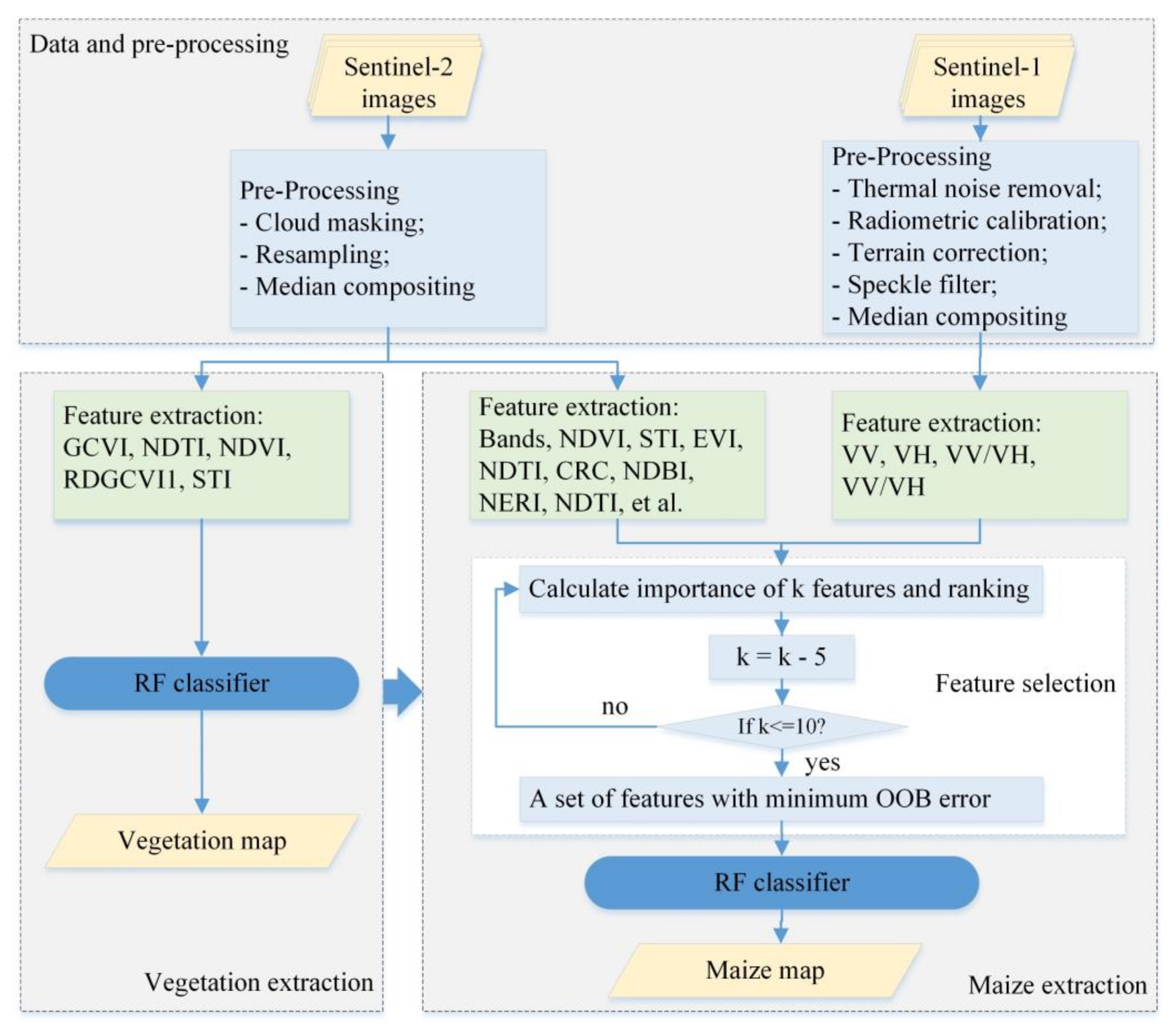
The methodology based on random forest classification is proposed to extract maize planting area, the detailed technical flow is shown schematically in Figure 2. The proposed methodology mainly consists of two steps:
Step I: Vegetation extraction. This is mainly to separate vegetation from non-vegetation to reduce the inter-class variance between maize/non-maize vegetation and non-vegetations. In this step, the RF classification model is constructed by using S2 time series and ground-based reference data, and the number of input indicators of RF is 30 (i.e., five spectral indices of GCVI, NDTI, NDVI, STI and RDGCVI1, each with six different dates from April to September). Only these five spectral indicators of S2 were selected because we found that these five indicators are more sensitive to vegetation and contribute the most to the extraction of vegetation regions in our previous study [63].
Step II: Maize extraction. The new RF classification model is trained by using S1 and S2 time-series images and ground-based reference data to distinguish between maize and non-maize vegetation in vegetation regions. In order to illustrate the necessity of introducing S1 data and the advantage of combined S1 and S2 data in crop mapping on highly complex and heterogeneous vegetation landscapes, three new RF models are developed by using indicators from S1 (alone), S2 (alone), and combination of S1 and S2 as the input of RF, respectively. The developed RF by using S1 (alone), S2 (alone) and the combined data are named as RF_S1, RF_S2, RF_S1&S2, respectively. The number of input indicators of these three RF models is 24 (i.e., four polarization characteristics of VV, VH, VV-VH, and VV/VH from S1 images, each with six different dates from April to September), 180 (i.e., all 30 indicators from S2 images, each indicator has six different dates from April to September), and 204 (i.e., combined indicators from both S1 and S2), respectively.
Considering that high-dimension input information may contain noise and redundancy, it will lead to over-fitting of a machine learning model. Thus, a specific feature selection procedure is essential to reduce information redundancy and prevent over-fitting when S2 (alone) or combined data are used to train a RF model. Embedded feature selection technique is embedding the feature selection process in the training of prediction models, which not only investigates the importance of input variables, but also gives the final prediction model [27], such as the feature selection strategy based on RF [30], in which the recursive variables elimination is used to reduce the computational complexity [64]. We adopt this RF-based embedded feature selection strategy to select a set of optimal feature variables with the smallest OOB error, wherein each iteration eliminates five features with the lowest importance until the number of features is less than 10 (Here, we set the threshold to 10 because we found that when the number of features is less than 10, the OOB error of the RF model begins to increase significantly), to establish the final RF maize extraction model with good generalization ability.
In our study, the sample dataset is divided into training set and validation set by a ratio of 8:2. The training set is used to train the RF classification model, and the independent validation set is used to examine the generalization performance of the developed RF model. Considering that the distribution of samples may be unbalanced, the stratified sampling method is adopted in the sample dataset division. The objective of RF model training process is to determine the optimal structure and hyperparameters to obtain the highest classification accuracy [65]. However, some previous studies have shown that different parameterization schemes have a limited influence on classification accuracy [57,66]. To reduce the computation cost and achieve a relatively good classification accuracy, the number of decision trees in the RF was set to 200, and the number of random feature variables was set to the square root of the total number of variables. Besides, the minimum number of terminal nodes was set to 10.

3.3. Accuracy Assessment

For quantitative evaluation of classification accuracy, most of the literature define a confusion matrix to calculate some evaluation indicators, such as overall accuracy, recall, precision, Kappa coefficient [67]. The confusion matrix was also constructed in this study, and five evaluation indexes, including recall (R), precision (P), overall accuracy (OA), F1_Score and Kappa coefficient, are calculated.
R = X i i i = 1 n X i +
P = X i i i = 1 n X + i
OA = i = 1 n X ii i = 1 n j = 1 n X i j
F 1 Score i = 2 × P × R P + R
Kappa = N i = 1 n X i i i = 1 n X i + × X + i N 2 i = 1 n X i + + X + i
where N represents the number of training samples, n represents the number of classification categories, and i represents a specific category. P quantifies the number of positive samples that actually belong to the positive category, and R quantifies the number of positive samples that have been correctly predicted. OA refers to the probability that a sample will be correctly classified. F1_Score is used to quantify the output quality of the model, which is the harmonic mean of P and R. The value of F1_score ranges from 0 to 1, and the closer it is to 1, the higher the classification accuracy of the model is. Kappa coefficient is an indicator for detecting and verifying the consistency between the actual categories and the predicted categories of samples. The value of Kappa is usually between 0 and 1, and the closer the value is to 1, the higher the consistency is.

4. Results

4.1. Vegetation Extraction Result

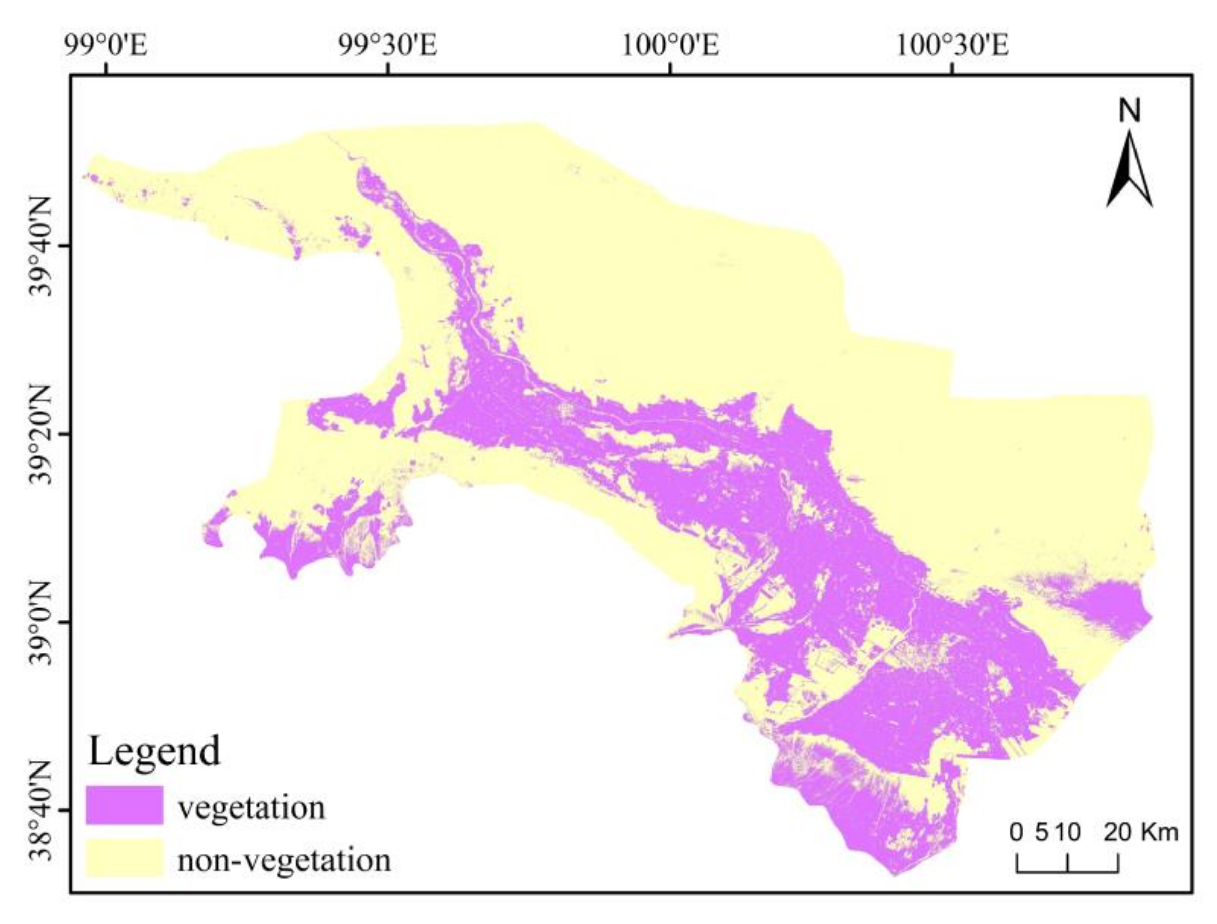
The RF classification model based on 30 input indicators from S2 can effectively classify vegetation and non-vegetation regions in the study area, as shown in Figure 3. It can be seen that 31% of the study area is covered by vegetation. The OA and Kappa coefficients of the developed RF classification model are 97.36% and 0.95, respectively. In addition, the OA, P, R, Kappa coefficient, and the F1_Scores of the model are 96%, 0.94, 0.98, 0.92, and 0.96, respectively, in the independent validation set.
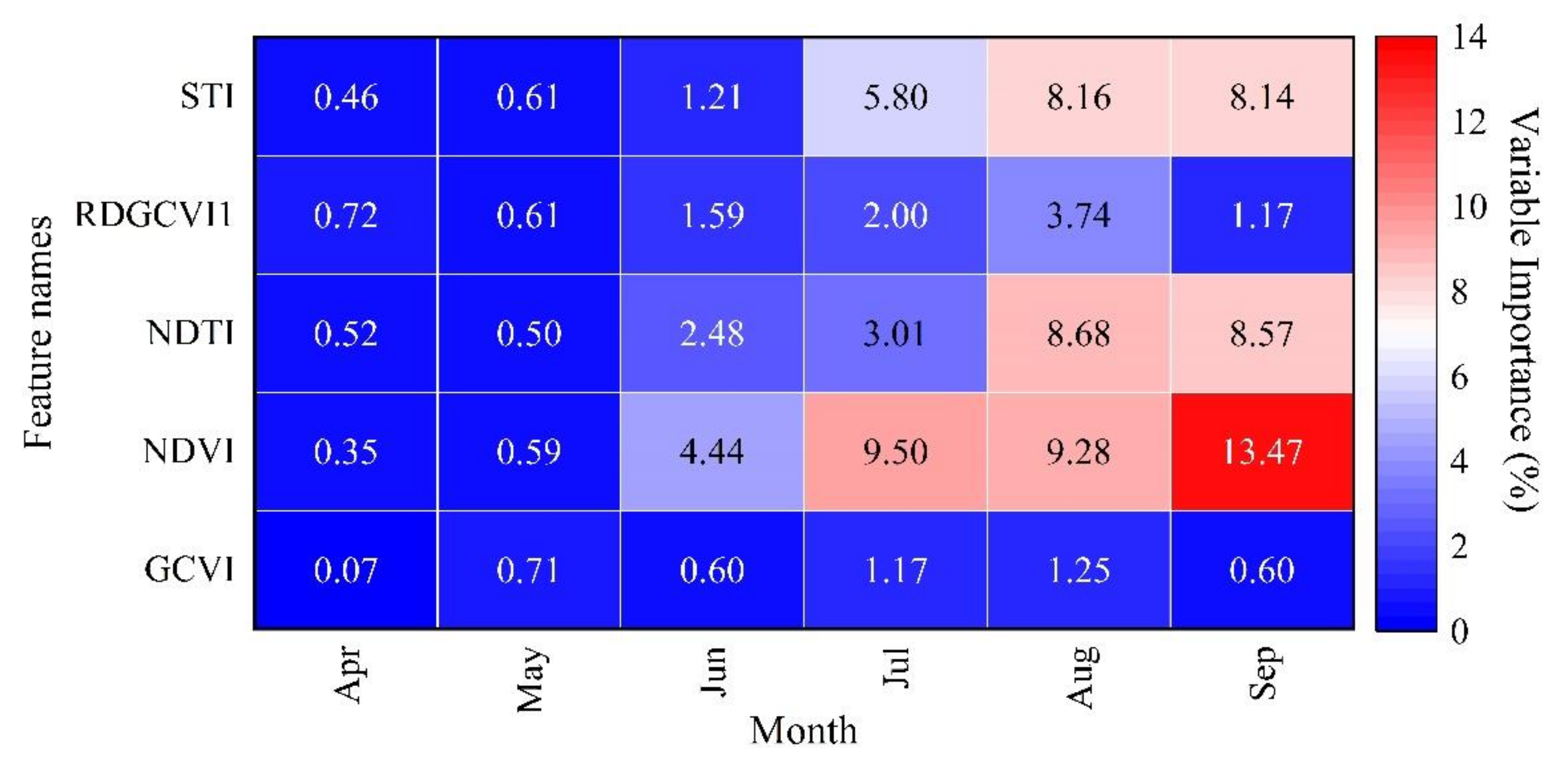
Meanwhile, the importance of the 30 input variables is also calculated by the RF model (Figure 4). The results indicate that the NDVI, NDTI and STI are the three most important variables in the vegetation extraction process, especially NDVI from July to September (i.e., NDVI_Jul, NDVI_Aug, and NDVI_Sep), and their importance values reach 9.50%, 9.28% and 13.47%, respectively. Thus, the NDVI is the dominant indicator to identify vegetation and non-vegetation. Moreover, the other seven relatively important indicators are NDTI_Aug, NDTI_Sep, STI_ Aug, STI_ Sep, STI_Jul, NDVI_Jun and RDGCVI1_ Aug. On the time scale, the importance of indicators is more vital in July, August, and September. This is consistent with the actual situation as there are obvious differences in spectral signals between vegetation and non-vegetation during the vegetation flourishes in these months.

4.2. Maize Extraction Result

4.2.1. The Optimal Features

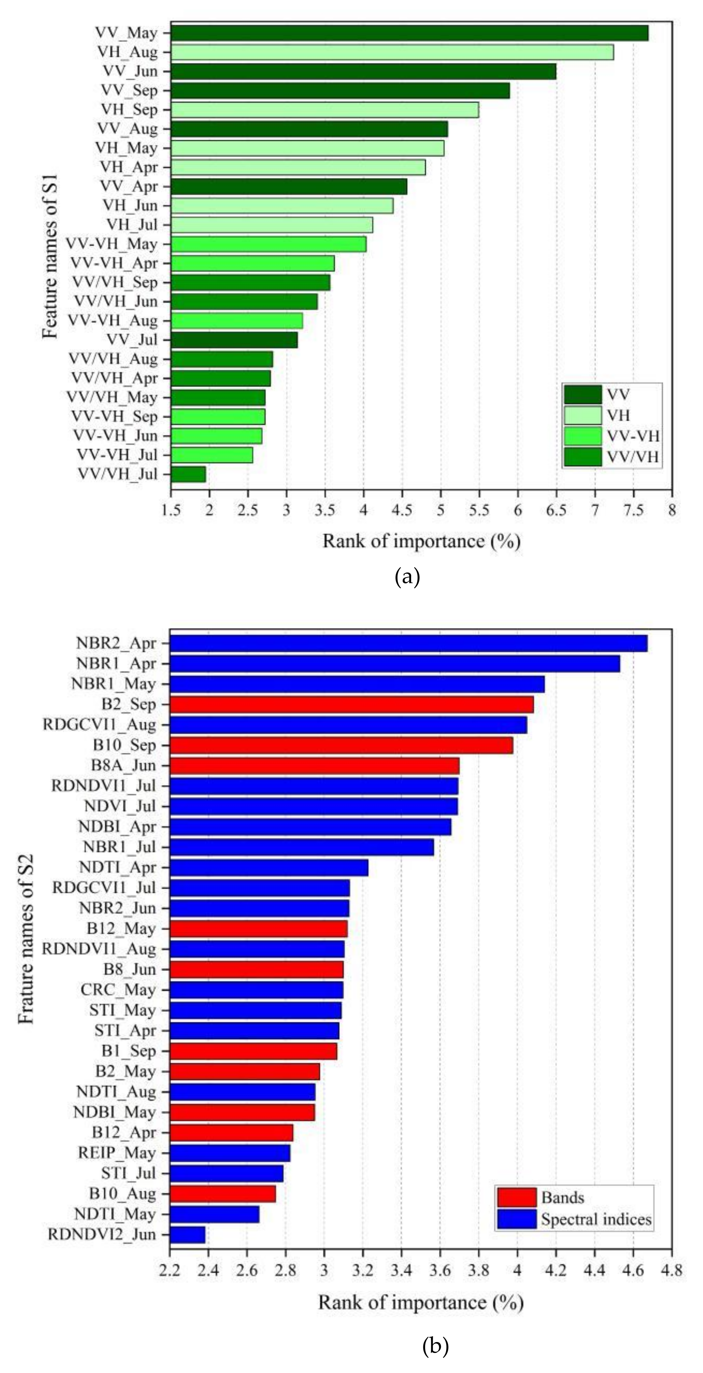
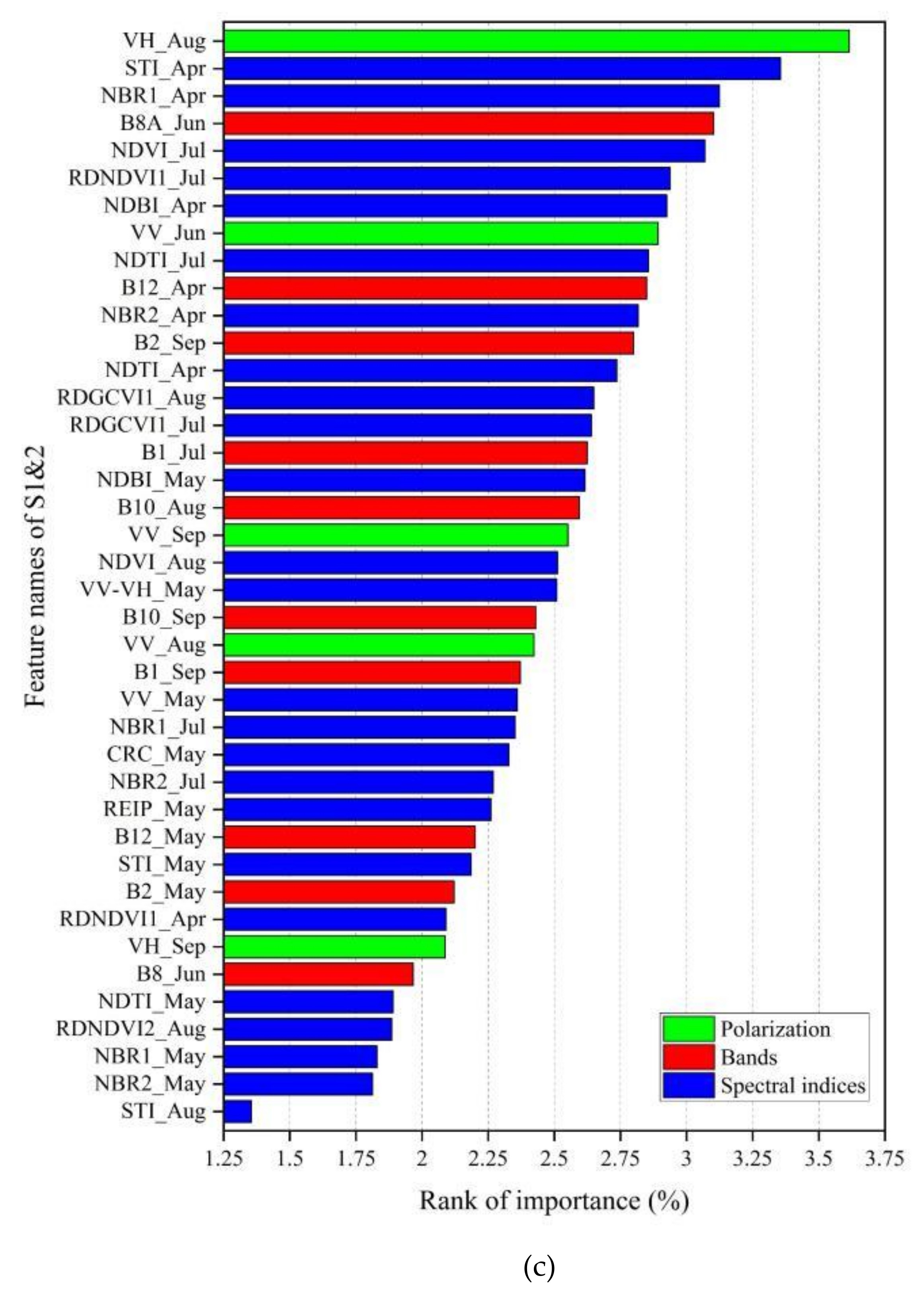
The results of feature selection show that the number of optimal features with the minimum OOB error is 30 and 40 for RF_S2 and RF_S1&S2 classification model, respectively. The 24 feature indicators of RF_S1 and the optimal features of RF_S2 and RF_S1&S2 are displayed in Figure 5.
Obviously, the RF_S1 model is extremely dependent on VV and VH polarization, and the top-10 features are the VV and VH polarization signals from May to September during the main growth period of crops, such as VV_May, VH_Aug, VV_Jun, VV_Sep, VH_Sep, VV_Aug, VH_May, VH_Apr, VV_Apr and VH_ Jun. The top-10 features of RF_S2 model include both band information and spectral indices from S2 images, where three band features are B2_Sep, B10_Sep and B8A_Jun, and seven spectral index features are NBR2_Apr, NBR1_Apr, NBR1_May, RDGCVI1_Aug, RDNDVI1_Jul, NDVI_Jul and NDBI_Apr. The optimal features of RF_S2 are relatively large, which may be related to the complex and heterogeneous surface coverage in the study area. The number of optimal features of RF_S1&2 model is the most, even up to 40, including polarization characteristics, band information and spectral indices, which may be related to the abundant spectral information that can more fully reflect complicated surface coverage. The top 10 features of RF_S1&S2 are 6 spectral indicators (i.e., STI_Apr, NBR1_Apr, NDVI_Jul, RDNDVI1_Jul, NDBI_Apr and NDTI_Jul), 2 polarization characteristics (i.e., VH_Aug and VV_Jun from S1), and 2 band indicators (i.e., B8A_Jun and B12_Apr from S2).
VV polarization contributed the most compared with other polarization in this study of maize planting area extraction based on S1 image. It can detect crop information better because of its strong penetrability. In the maize planting area extraction research based on S2 image, the contribution of NBR index is dominant, especially in April, which is related to the local cultivated land activities. Before planting crops in that year, farmers usually loosen the soil of the farmland and burn the roots left in the farmland in the previous year, which makes almost all farmland have their own unique NBR response. In general, the contribution of characteristic variables of S2 is greater than that of S1, which indicates that the bands and spectral indices from S2 image are more sensitive to crop information. However, unlike S1 (alone) and S2 (alone), the top three indicators are VH, STI, and NBR in descending order of importance. Combined with more spectral features and polarization patterns, the importance of variables will become difficult to explain.

4.2.2. Comparison of Maize Extraction Results from Three RF Models

The performance quantitative evaluation results of RF_S1, RF_S2 and RF_S1&S2 maize extraction models on the training set and the independent test set are shown in Table 2. On the training set, the OAs of these models are 86.42%, 88.39% and 89.46%, and Kappa coefficients are 0.72, 0.76 and 0.79, respectively. The OA, R, P, Kappa coefficients and F1_Score of RF_S1 are 80.14%, 0.76, 0.81, 0.6 and 0.78, respectively. Compared with RF_S1, the performance of RF_S2 has been improved significantly, and the OA, R, P, Kappa and F1_Score of RF_S2 are 85.51%, 0.82, 0.87, 0.71 and 0.84, respectively. This indicates that the multi-temporal S2 optical images are more suitable for maize extraction than the microwave S1 images in the study area. The various spectral indicators provided by S2 images can better identify the different phenological characteristics of different vegetation, which is beneficial to distinguish maize from other vegetation. The performance of RF_S1&S1 has been further improved, with the OA, R, P, Kappa and F1_Score are 87.63%, 0.84, 0.87, 0.75 and 0.86. This indicates that combining S1 and S2 data, the spatial information of the two can complement each other, so as to provide more comprehensive features and extract the maize cover more robustly and accurately.
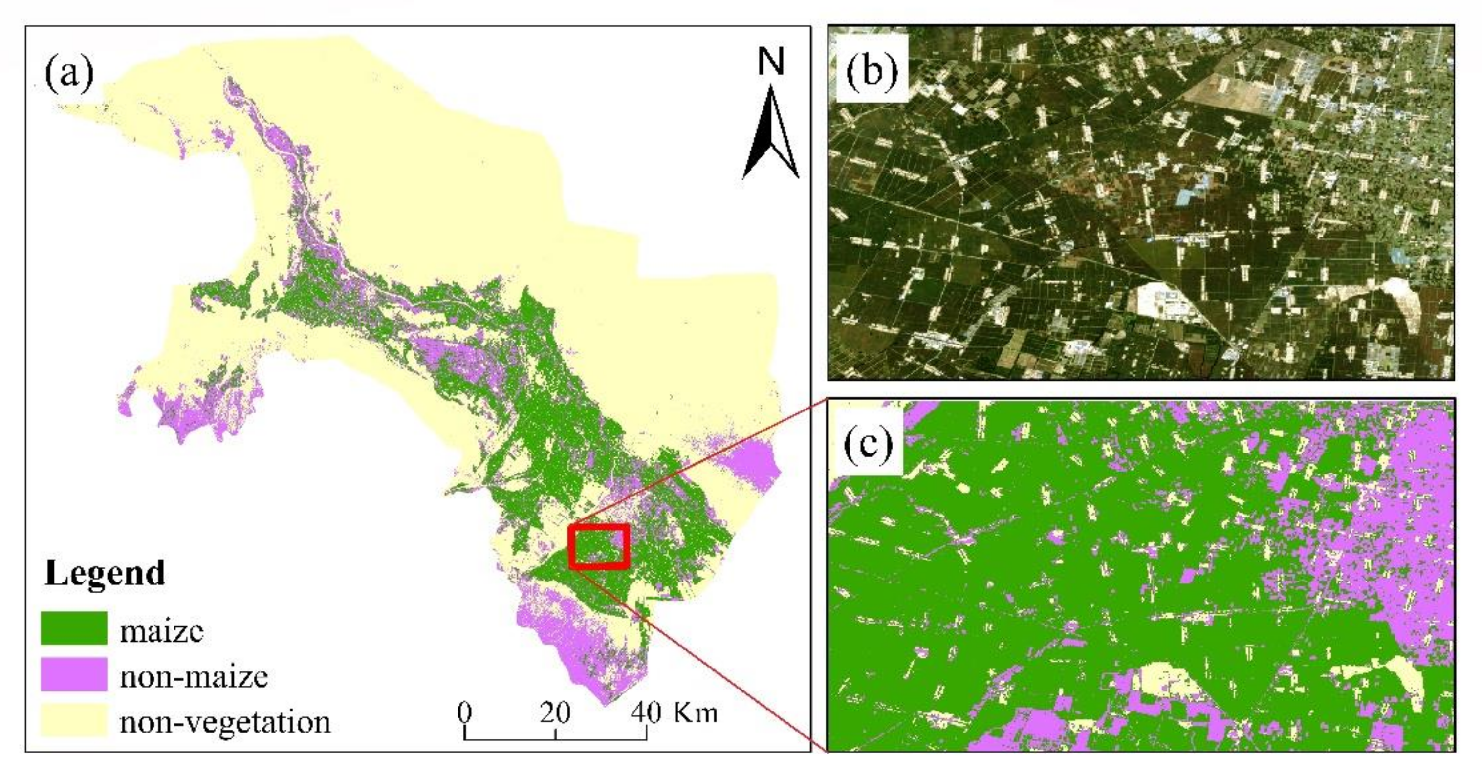
The distribution map of maize planting area extracted by RF_S1&S2 (the maize distribution maps extracted by RF_S1 and RF_S2 models are very close to RF_S1&S2, so we will not show them here) in the study area is shown in Figure 6. It can be seen from the figure that maize is mainly distributed in areas with flat terrain, close to water sources and well-developed irrigation systems (Figure 6a). In addition, there are a small number of mazes distributing in the northern, southwest and southern of the study area, which is consistent with the results of our field investigation. According to our field investigation, the cultivated land in the southern part of the study area is mainly terraced fields. Because these areas are difficult to irrigate, they are planted with forage maize that needs less water and is more drought resistant. Owing to the agricultural planting structure of the study area is the combination of modern agriculture and traditional agriculture, one of the important characteristics of corn distribution in the study area is relatively fragmented, such as the typical desert-oasis zone in the study area (i.e., local enlarged region as shown in Figure 6c), mixed distribution of corn, residential land, and greenhouse planting is found. In addition, the true color composite map of S2 image in the local enlarged area (Figure 6b) also shows that the surface heterogeneity of the area is very strong, and the surface coverage is very fragmented.

5. Discussion

5.1. Effects of Pre-processing on Maize Mapping

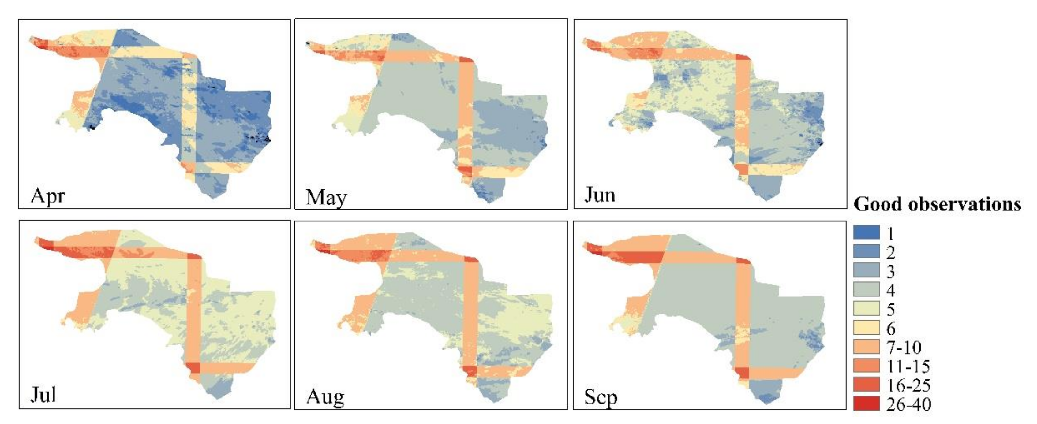
The quality of optical images and radar images is one of the keys to accurate extraction of maize planting area in this study. Because of the different dates of adjacent tracks and cloud contamination [52], the S2 time series images with different time intervals were composited using cloud mask algorithm and monthly median synthesis method. The QA60 band of S2 dedicated to monitoring cloud information was used in cloud masking processing. However, for time aggregation of S2 time series images, each scene will affect the final estimate [49]. Thus, the number of good observations (i.e., not polluted by cloud cover) on each pixel in the study area from April to September were recorded (Figure 7). As can be seen from the Figure 7, the number of good observations from July to September was significantly larger than from April to June. In particular, the number of good observations in April was less than or equal to 3. In addition, it is worth noting that a very small fraction of the pixels in the monthly median composite image of April and June were missing. To improve image quality and realize information reconstruction, moving median processing was adopted for S2 monthly median synthesis images [52]. To verify the effectiveness of the moving median processing, the RF classification models were constructed by using S2 images before and after moving median processing per month in April, May, and June. The accuracy of maize/non-maize classification is shown in Table 3. The results indicate that the classification accuracy is improved for RF models that were constructed by the moving median processed S2 data, with higher OA, Kappa, and F1_Score values in most cases.
Currently, S1 is the only radar satellite system that can provide a dense time series with global coverage. It is an excellent alternative data source for agricultural land cover maps. We used the 7 × 7 Refined Lee speckle filter, which can preserve the edges and present the preserved details [68] when filtering the image in uniform and non-uniform areas to reduce the speckle noise. We still take April, May, and June as examples to construct the corresponding RF classification models per month by using S1 data before and after the speckle filter, the maize/non-maize classification accuracy results (Table 3) indicate that the performance of constructed RF models is significantly improved in April and May after speckle filter. Although there was no improvement for RF model after speckle filter in June, there was no significant deterioration, which indicates that the Refined Lee speckle filter can improve the quality of S1 data effectively. Inglada et al. (2016) also discussed the influence of spectral filtering (e.g., with a simple 3 × 3 pixels filter window) on classification accuracy in the early crop type recognition, they found that the speckle filtering introduced a statistically significant small improvement [11], which is consistent with our research results.

5.2. Effects of Multi-Temporal Images on Maize Mapping

There are some limitations in extracting ground information from a single image. Due to the strong heterogeneity, high degree of fragmentation and various land cover types in the study area, there will always be the phenomenon of the same object with different spectra and different objects with the same spectrum for RS images. In addition, extracting crop distribution information from high-resolution RS imagery is much difficult than from the other resolution because high-resolution imagery exhibits more complex spectral character. This undoubtedly increases the difficulty of crops classification and makes the capability of applying single RS data on crops classification is reduced. Multi-temporal images can provide more spectral information [69], which seems to reduce misclassification greatly.
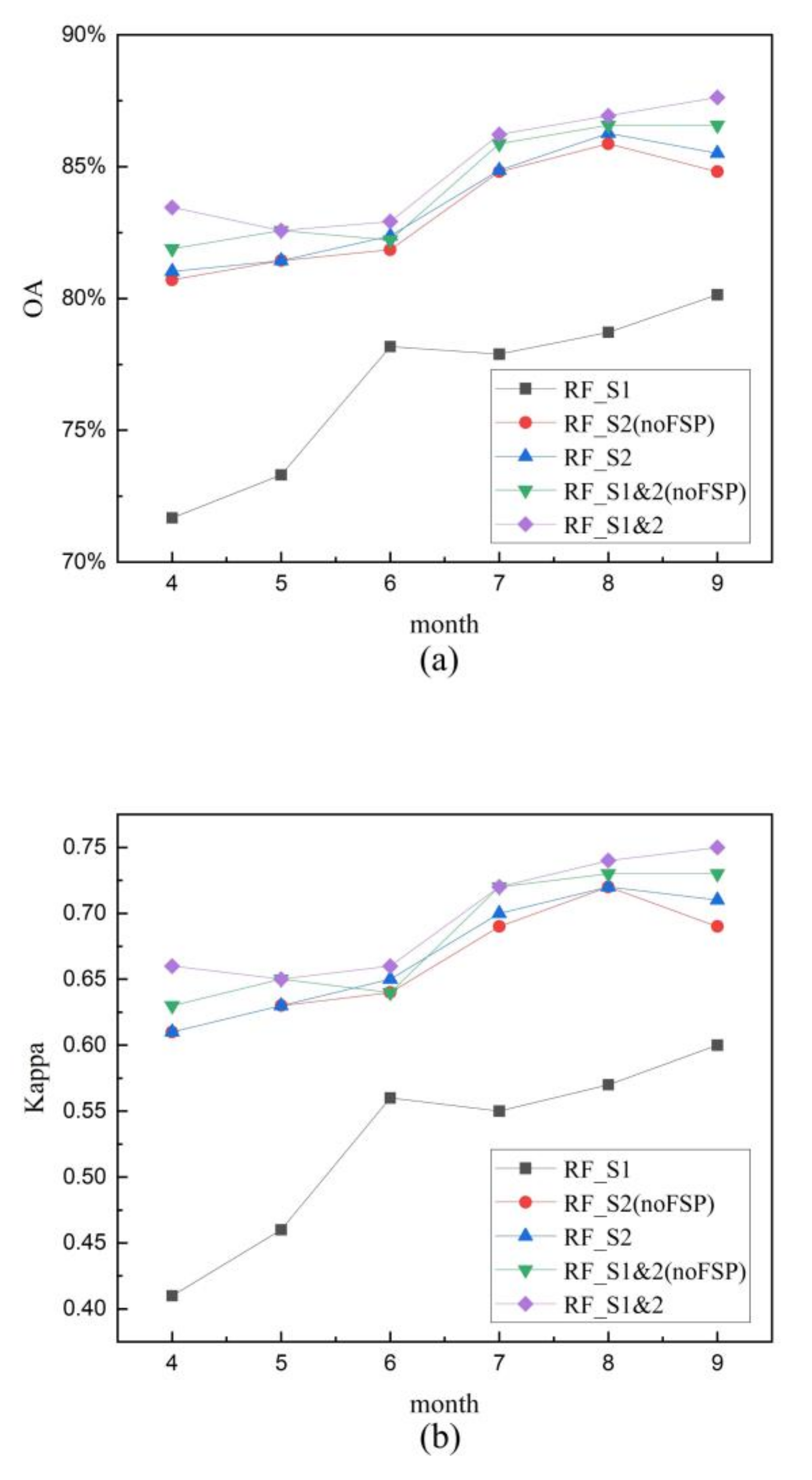
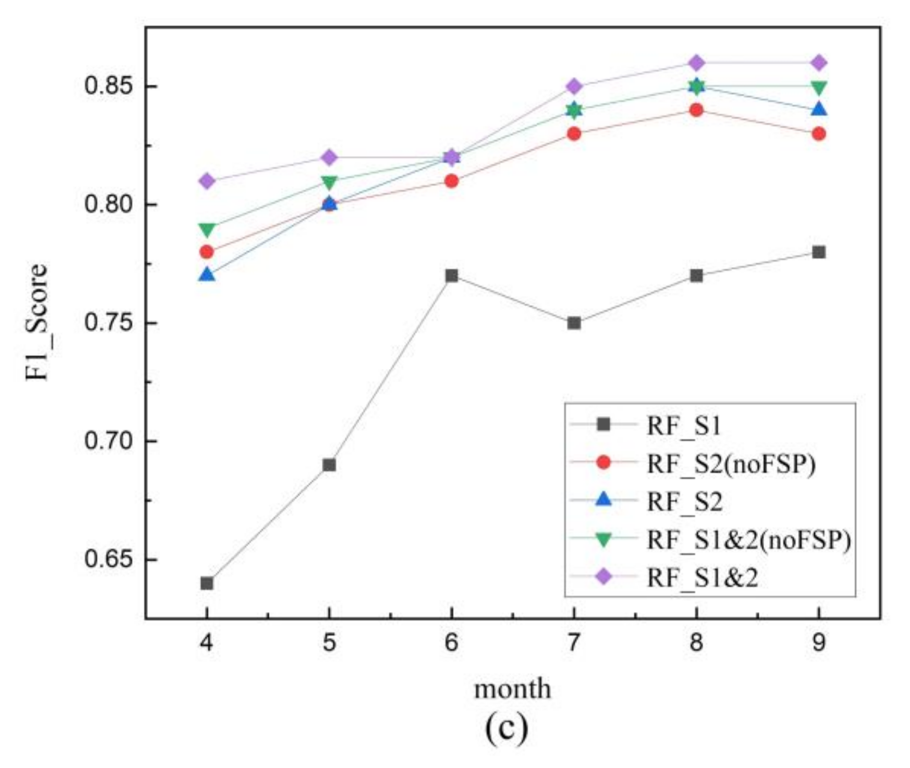
In this study, the incremental learning strategy is adopted to explore the impact of multi-temporal images on maize mapping accuracy. The incremental learning trains the initial model on the data subset and then continuously adds new data to update the model [30,70]. Thus, we train the initial RF models with the data (including S1 alone, S2 alone, and combined S1 and S2) of April as the data subset and validate these models to obtain the initial classification accuracy. Then, the next month’s data is introduced as the data subset in turn and retrain the RF models classification, and until the data of September is also introduced. The experiment results indicate that the classification accuracy of the RF models is steadily improved with the introduction of more temporal information (Figure 8), especially for the RF model that constructed by using S1 data alone, which is improved significantly wherein the information of May, August, June, and September is introduced. This may be due to the fact that these months are the seedling stage, milky stage, jointing stage and mature stage of maize, and the difference of SAR signals between maize and other surrounding ground objects are relatively large. The classification accuracy of the RF model is gradually improved from 72%, 0.41 and 0.64 of the initial models to 80.14%, 0.6, and 0.78 of the final models for OA, Kappa coefficient, and F1_Score, respectively, with the availability of more data. With respect to the impact of S1 images in early crop classification, our result is consistent with the study of Inglada et al. (2016), which shows that the classification accuracy is gradually improved with the evolution of seasons and more data available [11]. However, the classification accuracy of their study is slightly higher than ours (the maximum value of Kappa coefficient is about 0.675), this may be due to the use of many variables related to crop texture features. We also found that S1 images do not perform very well in the early maize planting area extraction, this is similar to the study of Demarez et al., (2019), which indicates that the classification accuracy of early crop is the lowest with Kappa ≈ 0.25, as their study did not conduct monthly synthesis processing for the multi-temporal images [30]. Nguyen et al., (2017) found that the dense SAR time series and phenological characteristics are very critical in the study of rice cropland monitoring with Sentinel-1 Data, and the Kappa coefficient can reach 0.76~0.87 [71]. Bargiel (2017) pointed that the detailed phenological information can be regarded as the foundation of crop classification in large regions, as the phenology varies with the different climate conditions in different regions [72]. In our study, the classification accuracy is somewhat low, which is related to the complex and heterogeneous vegetation structure in the study area. In the further classification study, we will consider the texture features of crops in this region.
The corresponding classification accuracy of RF model constructed by S2(alone) and combined S1&S2 data are significantly improved than that of S1(alone), which may be related to image characteristics since optical images generally understand the relationship between observations and vegetation phenology better than radar images [11]. Marais Sicre et al. (2016) indicate that the impact of crop classification accuracy mainly comes from available data and it is difficult to distinguish crop types accurately in the early stage of crop growth [73]. These results are consistent with the conclusions of Vuolo et al. (2018), indicating that classification accuracy is very poor (OA ≈ 50%) in the early stages of the crop growth [69]. However, relatively high accuracy (OA ≈ 81% ) was achieved at the very beginning of the crop growing season in our study, this may be related to the large number of spectral features we used is beneficial to crop classification. With the evolution of seasons, the maize classification accuracy increased significantly, and the accuracy of S2 based RF classification model achieves the best performance when the image information from May to August are all used as the model input, the OA, Kappa coefficient, and F1_Score values are 86.27%, 0.72, and 0.85, respectively. The classification accuracy of the corresponding RF model constructed by combined S1 and S2 data is further improved compared with that S2 (alone), this is consistent with the conclusion of Demarez et al., (2019), which indicates that the combination of optical data and SAR data can improve the precision of crop acreage extraction in highly heterogeneous regions [30]. The RF classification model achieves the best performance while all the available information is introduced, with the higher OA, Kappa coefficient, and F1_Score values even reach 87.63%, 0.75, and 0.86, respectively. Multi-temporal images of both optical S2 and/or S1 SAR can better capture the phenological information of different growth stages of maize, which is beneficial to crop classification in areas with complex vegetation structure and strong heterogeneity, this is also confirmed by Mercier et al., 2020, in which they indicate that the combined use of S1 and S2 was more accurate in identifying principal and secondary phenological stages for wheat and rapeseed mapping than using S1 or S2 data alone [74]. However, Mercier et al. (2019) also pointed out that the combination of S1 and S2 data has only a little improvement compared to those of S2 data alone, with Kappa coefficient appropriate 0.89 versus 0.87, in the study of land cover classification of forest-agriculture mosaic by using RF classifier [70], this study gives us a warning that whether S1 or S2 should be combined for classification research still needs specific analysis.

5.3. Effects of Feature Selection Procedure on Maize Mapping

The previous study of maize planting area extraction in Tanzania and Kenya [25] showed that the B1, STI, NDTI and shortwave infrared bands are the most important variables, which is consistent with the conclusion in our study area. In contrast, the importance of NBR1, NDVI and RDNDVI1 are stronger in our study area. In addition, the indicators from S1 (e.g., VV_May, VH_aug, VV_Jun, VV_Sep, and VH_Sep) are also of great importance in maize classification. The indicators from the near infrared band of S2 are the dominant contribution factors of maize classification in the study area. The importance of VV polarization is the most significant, and this conclusion can also be drawn from other crop classification studies [70]. However, some studies have shown that the index VH/VV can play an important role in crop classification due to it can reduce the impact of soil moisture and detect post-harvest spontaneous regrowth [48].
To explore the effect of the feature selection on maize mapping, we compared the RF models constructed by using S2 (alone) and combined S1 and S2 data with and without feature selection (Figure 8). We called the constructed RF model without feature selection procedure is a standard RF model, in which all the feature variables are involved in the training. Overall, the performance of RF models with the feature selection is slightly better than corresponding standard RF models. Meanwhile, the performance of standard RF model constructed by combined S1 and S2 is superior to that RF model constructed by S2 data alone with feature selection although the overall trend of classification accuracy for the RF models constructed by the combined S1 and S2 data is similar to that S2 data. However, as can be seen from the trend of Figure 8, the RF models with feature selection procedure are superior to the standard RF models. In short, it is very important to select the best feature and construct the appropriate RF model to improve the accuracy of maize classification in complex heterogeneous environment.

5.4. Uncertainty and Future Enhancement of Maize Mapping

Accurate ground truth data are crucial for training and validating classification algorithms [25], especially the quality of the training data is the key to obtaining satisfactory classification results [49]. The collection of sampling data is a major limitation of this study. Due to the limitation of sampling time in the field survey, there are fewer non-maize samples. Although non-maize samples were supplemented by Google earth image and S2 images, these samples may be biased and not representative enough, which may cause classification uncertainty.
Image quality is another key to obtaining satisfactory classification results. Cloud masking and moving median of processing of optical images and spectral filtering of radar images can significantly improve image quality, as described in Section 5.1. The Cloud or cirrus cover of S2 images was generally masked using the QA60 band [48,50]. Recent research found that clouds were masked more thoroughly using the Landsat simple cloud score algorithm than merely utilizing the QA60 quality assessment band [52]. In this algorithm, four bands and two spectral indices were used to compute cloud scores and detect clouds for S2 data. In our study, only moving median processing was used to eliminate the influence of clouds or cirrus clouds. However, the limitations of cloud masking may also still have contributed to the uncertainty of maize classification. Therefore, more attention should be paid to image pre-processing, especially to the cloud removal of optical images.
In the previous Section 4.2.2 and Section 5.2, we have confirmed that the RF models constructed by the combination of optical S2 data and S1 radar data have better classification accuracy than using either S1 or S2 data alone. This can be attributed to the complementary interaction of spatiotemporal information from multiple sources, which makes it possible to capture the surface ground objects’ feature features more completely. However, most of the previous studies have excluded the “atmospheric” bands, e.g., B1, B9, B10, of S2 [74], even though that information may also contribute to crop classification. In this study, we found that bands B1 and B10 of S2 or combined data have a non-negligible contribution in the process of maize classification (it can be seen in Section 4.2.1). This indicates that spectral reflectance from some atmospheric band is also related to crop growth and should be taken into account when establishing a crop classification model. Besides, the bands and artificial spectral indicator from S1 and S2 images used in this study may not represent the influence of complex factors, such as weather conditions and farming patterns. Thus, we need to further explore and extract other useful features in future maize classification study.
In addition, more advanced deep learning methods, such as convolutional neural networks, recursive neural networks, and long short-term memory networks, are also very popular methods in agricultural crop classification study recently [75,76]. Judging from the performance of existing research, deep learning seems to have more potential advantages than classic machine learning methods. This is because the features of traditional machine learning are manually screened, whereas deep learning technology can automatically mine the spatiotemporal information contained in the RS images. However, there is also a study that confirms that the long short-term memory network is similar to the random forest without significantly improvement for maize planting area mapping in the Liangzhou district of Gansu province, China [77]. Therefore, both RF and deep learning techniques need further in-depth study in the application of crop mapping.

6. Conclusions

This study explores how to use the combined high-resolution multi-temporal optical S2 and/or S1 SAR images to map the maize planting area in the middle reaches of the Heihe River basin via RF classification model with a feature selection procedure. The results revealed the multi-source RS images have the potential to provide more complementary feature information and improve the accuracy of maize mapping under the condition of complex and heterogeneous landscapes. The maize mapping accuracy of RF model constructed by using the combined S1 and S2 data was higher than that either S1 (alone) or S2 (alone), with OA of 87.63%, Kappa coefficient of 0.75, and F1_Sccore of 0.86. Compared with single temporal image, multi-temporal images can improve the abundance of input information of RF model and then improve the accuracy of classification. Besides, the optimal feature selection is also the key to improve the accuracy of maize mapping in the study area, which can effectively eliminate the redundant information led by a large number of similar or related input features, and reduce the possibility of over-fitting and then improve the classification accuracy of RF model. The proposed method in this study is suitable for fine classification of crops in highly complex and heterogeneous areas.

Author Contributions

Conceptualization, C.H., J.H., Y.Z. and Y.C.; Methodology, C.H., J.H., and Y.C.; Software, Y.C.; Formal analysis, Y.C.; Investigation, X.L. and Y.C.; Writing—Original Draft Preparation, Y.C.; Writing—Review and Editing, J.H. and Y.C. All authors have read and agreed to the published version of the manuscript.

Funding

This work is supported by the Strategic Priority Research Program of the Chinese Academy of Sciences “CAS Earth Big Data Science Project” (grant No. XDA19040504) and the National Natural Science Foundation of China under Grants (Project No. 41971326 and 41801271).

Conflicts of Interest

The authors declare no conflict of interest.

References

  1. Peña-Barragán, J.M.; Ngugi, M.K.; Plant, R.E.; Six, J. Object-based crop identification using multiple vegetation indices, textural features and crop phenology. Remote Sens. Environ. 2011, 115, 1301–1316. [Google Scholar] [CrossRef]
  2. Song, Q.; Hu, Q.; Zhou, Q.; Hovis, C.; Xiang, M.; Tang, H.; Wu, W. In-Season Crop Mapping with GF-1/WFV Data by Combining Object-Based Image Analysis and Random Forest. Remote Sens. 2017, 9, 1184. [Google Scholar] [CrossRef] [Green Version]
  3. Muhammad, S.; Zhan, Y.; Wang, L.; Hao, P.; Niu, Z. Major crops classification using time series MODIS EVI with adjacent years of ground reference data in the US state of Kansas. Optik 2016, 127, 1071–1077. [Google Scholar] [CrossRef]
  4. Skakun, S.; Franch, B.; Vermote, E.; Roger, J.C.; Becker-Reshef, I.; Justice, C.; Kussul, N. Early season large-area winter crop mapping using MODIS NDVI data, growing degree days information and a Gaussian mixture model. Remote Sens. Environ. 2017, 195, 244–258. [Google Scholar] [CrossRef]
  5. Son, N.T.; Chen, C.F.; Chen, C.R.; Guo, H.Y. Classification of multitemporal Sentinel-2 data for field-level monitoring of rice cropping practices in Taiwan. Adv. Space Res. 2020, 65, 1910–1921. [Google Scholar] [CrossRef]
  6. Ajadi, O.A.; Barr, J.; Liang, S.Z.; Ferreira, R.; Kumpatla, S.P.; Patel, R.; Swatantran, A. Large-scale crop type and crop area mapping across Brazil using synthetic aperture radar and optical imagery. Int. J. Appl. Earth Obs. Geoinf. 2021, 97, 102294. [Google Scholar] [CrossRef]
  7. Minasny, B.; Shah, R.M.; Che Soh, N.; Arif, C.; Indra Setiawan, B. Automated Near-Real-Time Mapping and Monitoring of Rice Extent, Cropping Patterns, and Growth Stages in Southeast Asia Using Sentinel-1 Time Series on a Google Earth Engine Platform. Remote Sens. 2019, 11, 1666. [Google Scholar] [CrossRef] [Green Version]
  8. Mascolo, L.; Lopez-Sanchez, J.M.; Vicente-Guijalba, F.; Nunziata, F.; Migliaccio, M.; Mazzarella, G. A Complete Procedure for Crop Phenology Estimation With PolSAR Data Based on the Complex Wishart Classifier. IEEE Trans. Geosci. Remote Sens. 2016, 54, 6505–6515. [Google Scholar] [CrossRef] [Green Version]
  9. Arias, M.; Campo-Bescós, M.Á.; Álvarez-Mozos, J. Crop Classification Based on Temporal Signatures of Sentinel-1 Observations over Navarre Province, Spain. Remote Sens. 2020, 12, 0278. [Google Scholar] [CrossRef] [Green Version]
  10. Erinjery, J.J.; Singh, M.; Kent, R. Mapping and assessment of vegetation types in the tropical rainforests of the Western Ghats using multispectral Sentinel-2 and SAR Sentinel-1 satellite imagery. Remote Sens. Environ. 2018, 216, 345–354. [Google Scholar] [CrossRef]
  11. Inglada, J.; Vincent, A.; Arias, M.; Marais-Sicre, C. Improved Early Crop Type Identification By Joint Use of High Temporal Resolution SAR And Optical Image Time Series. Remote Sens. 2016, 8, 362. [Google Scholar] [CrossRef] [Green Version]
  12. Cai, Y.; Lin, H.; Zhang, M. Mapping paddy rice by the object-based random forest method using time series Sentinel-1/Sentinel-2 data. Adv. Space Res. 2019, 64, 2233–2244. [Google Scholar] [CrossRef]
  13. Filella, I.; Penuelas, J. The red edge position and shape as indicators of plant chlorophyll content, biomass and hydric status. Int. J. Remote Sens. 1994, 15, 1459–1470. [Google Scholar] [CrossRef]
  14. Schlerf, M.; Atzberger, C.; Hill, J. Remote sensing of forest biophysical variables using HyMap imaging spectrometer data. Remote Sens. Environ. 2005, 95, 177–194. [Google Scholar] [CrossRef] [Green Version]
  15. Panda, S.S.; Ames, D.P.; Panigrahi, S. Application of vegetation indices for agricultural crop yield prediction using neural network techniques. Remote Sens. 2010, 2, 673–696. [Google Scholar] [CrossRef] [Green Version]
  16. Reed, B.C.; Brown, J.F.; VanderZee, D.; Loveland, T.R.; Merchant, J.W.; Ohlen, D.O. Measuring phenological variability from satellite imagery. J. Veg. Sci. 1994, 5, 703–714. [Google Scholar] [CrossRef]
  17. Huemmrich, K.F.; Privette, J.L.; Mukelabai, M.; Myneni, R.B.; Knyazikhin, Y. Time-series validation of MODIS land biophysical products in a Kalahari woodland, Africa. Int. J. Remote Sens. 2007, 26, 4381–4398. [Google Scholar] [CrossRef]
  18. Huete, A.; Liu, H.; Batchily, K.; Van Leeuwen, W. A comparison of vegetation indices over a global set of TM images for EOS-MODIS. Remote Sens. Environ. 1997, 59, 440–451. [Google Scholar] [CrossRef]
  19. Jeong, S.; Kang, S.; Jang, K.; Lee, H.; Hong, S.; Ko, D. Development of Variable Threshold Models for detection of irrigated paddy rice fields and irrigation timing in heterogeneous land cover. Agric. Water Manag. 2012, 115, 83–91. [Google Scholar] [CrossRef]
  20. Huete, A.; Didan, K.; Miura, T.; Rodriguez, E.P.; Gao, X.; Ferreira, L.G. Overview of the radiometric and biophysical performance of the MODIS vegetation indices. Remote Sens. Environ. 2002, 83, 195–213. [Google Scholar] [CrossRef]
  21. Van Deventer, A.; Ward, A.; Gowda, P.; Lyon, J. Using thematic mapper data to identify contrasting soil plains and tillage practices. Photogramm. Eng. Rem. S. 1997, 63, 87–93. [Google Scholar] [CrossRef]
  22. Roy, D.P.; Boschetti, L.; Trigg, S.N. Remote Sensing of Fire Severity: Assessing the Performance of the Normalized Burn Ratio. IEEE Geosci. Remote Sens. Lett. 2006, 3, 112–116. [Google Scholar] [CrossRef] [Green Version]
  23. Benbahria, Z.; Sebari, I.; Hajji, H.; Smiej, M.F. Automatic Mapping of Irrigated Areas in Mediteranean Context Using Landsat 8 Time Series Images and Random Forest Algorithm. In Proceedings of the IGARSS 2018-2018 IEEE International Geoscience and Remote Sensing Symposium, Valencia, Spain, 22–27 July 2018; pp. 7986–7989. [Google Scholar]
  24. Bannari, A.; Morin, D.; Bonn, F.; Huete, A. A review of vegetation indices. Remote Sens. 1995, 13, 95–120. [Google Scholar] [CrossRef]
  25. Jin, Z.; Azzari, G.; You, C.; Di Tommaso, S.; Aston, S.; Burke, M.; Lobell, D.B. Smallholder maize area and yield mapping at national scales with Google Earth Engine. Remote Sens. Environ. 2019, 228, 115–128. [Google Scholar] [CrossRef]
  26. Kishino, M.; Tanaka, A.; Ishizaka, J. Retrieval of Chlorophyll a, suspended solids, and colored dissolved organic matter in Tokyo Bay using ASTER data. Remote Sens. Environ. 2005, 99, 66–74. [Google Scholar] [CrossRef]
  27. Saeys, Y.; Inza, I.; Larrañaga, P. A review of feature selection techniques in bioinformatics. Bioinformatics 2007, 23, 2507–2517. [Google Scholar] [CrossRef] [Green Version]
  28. Li, Q.; Wang, C.; Zhang, B.; Lu, L. Object-Based Crop Classification with Landsat-MODIS Enhanced Time-Series Data. Remote Sens. 2015, 7, 16091–16107. [Google Scholar] [CrossRef] [Green Version]
  29. Hao, P.; Zhan, Y.; Wang, L.; Niu, Z.; Shakir, M. Feature Selection of Time Series MODIS Data for Early Crop Classification Using Random Forest: A Case Study in Kansas, USA. Remote Sens. 2015, 7, 5347–5369. [Google Scholar] [CrossRef] [Green Version]
  30. Demarez, V.; Helen, F.; Marais-Sicre, C.; Baup, F. In-Season Mapping of Irrigated Crops Using Landsat 8 and Sentinel-1 Time Series. Remote Sens. 2019, 11, 118. [Google Scholar] [CrossRef] [Green Version]
  31. Zhang, X.; Sun, Y.; Shang, K.; Zhang, L.; Wang, S. Crop Classification Based on Feature Band Set Construction and Object-Oriented Approach Using Hyperspectral Images. IEEE J-STARS. 2016, 9, 4117–4128. [Google Scholar] [CrossRef]
  32. Yin, L.; You, N.; Zhang, G.; Huang, J.; Dong, J. Optimizing Feature Selection of Individual Crop Types for Improved Crop Mapping. Remote Sens. 2020, 12, 0162. [Google Scholar] [CrossRef] [Green Version]
  33. Wang, S.; Azzari, G.; Lobell, D.B. Crop type mapping without field-level labels: Random forest transfer and unsupervised clustering techniques. Remote Sens. Environ. 2019, 222, 303–317. [Google Scholar] [CrossRef]
  34. Basukala, A.K.; Oldenburg, C.; Schellberg, J.; Sultanov, M.; Dubovyk, O. Towards improved land use mapping of irrigated croplands: Performance assessment of different image classification algorithms and approaches. Eur. J. Remote Sens. 2017, 50, 187–201. [Google Scholar] [CrossRef] [Green Version]
  35. Moumni, A.; Lahrouni, A. Machine Learning-Based Classification for Crop-Type Mapping Using the Fusion of High-Resolution Satellite Imagery in a Semiarid Area. Scientifica 2021, 2021, 8810279. [Google Scholar] [CrossRef]
  36. Gilbertson, J.K.; Kemp, J.; van Niekerk, A. Effect of pan-sharpening multi-temporal Landsat 8 imagery for crop type differentiation using different classification techniques. Comput. Electron. Agric. 2017, 134, 151–159. [Google Scholar] [CrossRef] [Green Version]
  37. Zhang, H.; Kang, J.; Xu, X.; Zhang, L. Accessing the temporal and spectral features in crop type mapping using multi-temporal Sentinel-2 imagery: A case study of Yi’an County, Heilongjiang province, China. Comput. Electron. Agric. 2020, 176, 105618. [Google Scholar] [CrossRef]
  38. Sun, C.; Bian, Y.; Zhou, T.; Pan, J. Using of Multi-Source and Multi-Temporal Remote Sensing Data Improves Crop-Type Mapping in the Subtropical Agriculture Region. Sensors 2019, 19, 2401. [Google Scholar] [CrossRef] [PubMed] [Green Version]
  39. Biradar, C.M.; Thenkabail, P.S.; Noojipady, P.; Li, Y.; Dheeravath, V.; Turral, H.; Velpuri, M.; Gumma, M.K.; Gangalakunta, O.R.P.; Cai, X.L.; et al. A global map of rainfed cropland areas (GMRCA) at the end of last millennium using remote sensing. Int. J. Appl. Earth Obs. 2009, 11, 114–129. [Google Scholar] [CrossRef]
  40. Ragettli, S.; Herberz, T.; Siegfried, T. An Unsupervised Classification Algorithm for Multi-Temporal Irrigated Area Mapping in Central Asia. Remote Sens. 2018, 10, 1823. [Google Scholar] [CrossRef] [Green Version]
  41. Biggs, T.W.; Thenkabail, P.S.; Gumma, M.K.; Scott, C.A.; Parthasaradhi, G.R.; Turral, H.N. Irrigated area mapping in heterogeneous landscapes with MODIS time series, ground truth and census data, Krishna Basin, India. Int. J. Remote Sens. 2007, 27, 4245–4266. [Google Scholar] [CrossRef]
  42. Wardlow, B.D.; Egbert, S.L. Large-area crop mapping using time-series MODIS 250 m NDVI data: An assessment for the U.S. Central Great Plains. Remote Sens. Environ. 2008, 112, 1096–1116. [Google Scholar] [CrossRef]
  43. Chen, Y.; Lu, D.; Luo, L.; Pokhrel, Y.; Deb, K.; Huang, J.; Ran, Y. Detecting irrigation extent, frequency, and timing in a heterogeneous arid agricultural region using MODIS time series, Landsat imagery, and ancillary data. Remote Sens. Environ. 2018, 204, 197–211. [Google Scholar] [CrossRef]
  44. Lu, L.; Cheng, G.; Li, X. Landscape change in the middle reaches of Heihe River Basin. J. Appl. Ecol. 2001, 1, 68–74, PMID: 11813437. [Google Scholar]
  45. Wang, S.; Ma, C.; Zhao, Z.; Wei, L. Estimation of Soil Moisture of Agriculture Field in the Middle Reaches of the Heihe River Basin based on Sentinel-1 and Landsat 8 Imagery. Remote Sens. Technol. Appl. 2020, 35, 13–22. [Google Scholar]
  46. Jiao, Y.; Ma, M.; Xiao, D. Landscape Pattern of Zhangye Oasis in the Middle Reaches of Heihe River Basin. J. Glaciol. Geocryol. 2003, 25, 94–99. [Google Scholar] [CrossRef]
  47. Zheng, L.; Tan, M. Comparison of crop water use efficiency and direction of planting structure adjustment in the middle reaches of Heihe River. J. Geo Inf. Sci. 2016, 18, 977–986. [Google Scholar] [CrossRef]
  48. Veloso, A.; Mermoz, S.; Bouvet, A.; Le Toan, T.; Planells, M.; Dejoux, J.F.; Ceschia, E. Understanding the temporal behavior of crops using Sentinel-1 and Sentinel-2-like data for agricultural applications. Remote Sens. Environ. 2017, 199, 415–426. [Google Scholar] [CrossRef]
  49. Carrasco, L.; O’Neil, A.; Morton, R.; Rowland, C. Evaluating Combinations of Temporally Aggregated Sentinel-1, Sentinel-2 and Landsat 8 for Land Cover Mapping with Google Earth Engine. Remote Sens. 2019, 11, 0288. [Google Scholar] [CrossRef] [Green Version]
  50. Slagter, B.; Tsendbazar, N.E.; Vollrath, A.; Reiche, J. Mapping wetland characteristics using temporally dense Sentinel-1 and Sentinel-2 data: A case study in the St. Lucia wetlands, South Africa. Int. J. Earth Obs. 2020, 86, 102009. [Google Scholar] [CrossRef]
  51. Fauvel, M.; Lopes, M.; Dubo, T.; Rivers-Moore, J.; Frison, P.L.; Gross, N.; Ouin, A. Prediction of plant diversity in grasslands using Sentinel-1 and -2 satellite image time series. Remote Sens. Environ. 2020, 237, 111536. [Google Scholar] [CrossRef]
  52. You, N.; Dong, J. Examining earliest identifiable timing of crops using all available Sentinel 1/2 imagery and Google Earth Engine. ISPRS J. Photogramm. 2020, 161, 109–123. [Google Scholar] [CrossRef]
  53. Gatti, A.; Bertolini, A. Sentinel-2 Products Specification Document. Available online: https://earth.esa.int/documents/247904/685211/Sentinel-2-Products-Specification-Document (accessed on 23 February 2015).
  54. Breiman, L. Random forests. Mach. Learn. 2001, 45, 5–32. [Google Scholar] [CrossRef] [Green Version]
  55. Breiman, L. Bagging predictors. Mach. Learn. 1996, 24, 123–140. [Google Scholar] [CrossRef] [Green Version]
  56. Belgiu, M.; Drăguţ, L. Random forest in remote sensing: A review of applications and future directions. ISPRS J. Photogramm. 2016, 114, 24–31. [Google Scholar] [CrossRef]
  57. Pelletier, C.; Valero, S.; Inglada, J.; Champion, N.; Dedieu, G. Assessing the robustness of Random Forests to map land cover with high resolution satellite image time series over large areas. Remote Sens. Environ. 2016, 187, 156–168. [Google Scholar] [CrossRef]
  58. Teluguntla, P.; Thenkabail, P.S.; Oliphant, A.; Xiong, J.; Gumma, M.K.; Congalton, R.G.; Yadav, K.; Huete, A. A 30-m landsat-derived cropland extent product of Australia and China using random forest machine learning algorithm on Google Earth Engine cloud computing platform. ISPRS J. Photogramm. 2018, 144, 325–340. [Google Scholar] [CrossRef]
  59. Chen, Z. Mapping plastic-mulched farmland with multi-temporal Landsat-8 data. Remote Sens. 2017, 9, 557. [Google Scholar] [CrossRef] [Green Version]
  60. Rodriguez-Galiano, V.F.; Ghimire, B.; Rogan, J.; Chica-Olmo, M.; Rigol-Sanchez, J.P. An assessment of the effectiveness of a random forest classifier for land-cover classification. ISPRS J. Photogramm. 2012, 67, 93–104. [Google Scholar] [CrossRef]
  61. Díaz-Uriarte, R.; Alvarez de Andrés, S. Gene selection and classification of microarray data using random forest. BMC Bioinform. 2006, 7, 3. [Google Scholar] [CrossRef] [Green Version]
  62. Genuer, R.; Poggi, J.M.; Tuleau-Malot, C. Variable selection using random forests. Pattern Recognit. Lett. 2010, 31, 2225–2236. [Google Scholar] [CrossRef] [Green Version]
  63. Chen, Y.; Huang, C.; Hou, J.; Han, W.; Feng, Y.; Li, X.; Wang, J. Extraction of Maize Planting Area based on Multi-temporal Sentinel-2 Imagery in the Middle Reaches of Heihe River. Remote Sens. Technol. Appl. 2021, 36, 340–347. [Google Scholar] [CrossRef]
  64. Guyon, I.; Weston, J.; Barnhill, S.; Vapnik, V. Gene Selection for Cancer Classification using Support Vector Machines. Mach. Learn. 2002, 46, 389–422. [Google Scholar] [CrossRef]
  65. Zhao, H.; Chen, Z.; Jiang, H.; Jing, W.; Sun, L.; Feng, M. Evaluation of Three Deep Learning Models for Early Crop Classification Using Sentinel-1A Imagery Time Series—A Case Study in Zhanjiang, China. Remote Sens. 2019, 11, 2673. [Google Scholar] [CrossRef] [Green Version]
  66. Thanh Noi, P.; Kappas, M. Comparison of random forest, k-nearest neighbor, and support vector machine classifiers for land cover classification using Sentinel-2 imagery. Sensors 2018, 18, 18. [Google Scholar] [CrossRef] [Green Version]
  67. Minh, H.V.T.; Avtar, R.; Mohan, G.; Misra, P.; Kurasaki, M. Monitoring and Mapping of Rice Cropping Pattern in Flooding Area in the Vietnamese Mekong Delta Using Sentinel-1A Data: A Case of An Giang Province. ISPRS Int. J. Geoinf. 2019, 8, 0211. [Google Scholar] [CrossRef] [Green Version]
  68. Shamsoddini, A.; Trinder, J.C. Edge-detection-based filter for SAR speckle noise reduction. Int. J. Remote Sens. 2012, 33, 2296–2320. [Google Scholar] [CrossRef]
  69. Vuolo, F.; Neuwirth, M.; Immitzer, M.; Atzberger, C.; Ng, W.T. How much does multi-temporal Sentinel-2 data improve crop type classification? Int. J. Appl. Earth Obs. 2018, 72, 122–130. [Google Scholar] [CrossRef]
  70. Mercier, A.; Betbeder, J.; Rumiano, F.; Baudry, J.; Gond, V.; Blanc, L.; Bourgoin, C.; Cornu, G.; Ciudad, C.; Marchamalo, M.; et al. Evaluation of Sentinel-1 and 2 Time Series for Land Cover Classification of Forest–Agriculture Mosaics in Temperate and Tropical Landscapes. Remote Sens. 2019, 11, 0979. [Google Scholar] [CrossRef] [Green Version]
  71. Nguyen, D.B.; Wagner, W. European Rice Cropland Mapping with Sentinel-1 Data: The Mediterranean Region Case Study. Water 2017, 9, 0392. [Google Scholar] [CrossRef]
  72. Bargiel, D. A new method for crop classification combining time series of radar images and crop phenology infor-mation. Remote Sen. Environ. 2017, 198, 369–383. [Google Scholar] [CrossRef]
  73. Marais Sicre, C.; Inglada, J.; Fieuzal, R.; Baup, F.; Valero, S.; Cros, J.; Huc, M.; Demarez, V. Early Detection of Summer Crops Using High Spatial Resolution Optical Image Time Series. Remote Sen. 2016, 8, 0591. [Google Scholar] [CrossRef] [Green Version]
  74. Mercier, A.; Betbeder, J.; Baudry, J.; Le Roux, V.; Spicher, F.; Lacoux, J.; Roger, D.; Hubert-Moy, L. Evaluation of Sentinel-1 & 2 time series for predicting wheat and rapeseed phenological stages. ISPRS J. Photogramm. 2020, 163, 231–256. [Google Scholar] [CrossRef]
  75. Kussul, N.; Lavreniuk, M.; Skakun, S.; Shelestov, A. Deep Learning Classification of Land Cover and Crop Types Using Remote Sensing Data. IEEE Geosci. Remote Sens. Lett. 2017, 14, 778–782. [Google Scholar] [CrossRef]
  76. Interdonato, R.; Ienco, D.; Gaetano, R.; Ose, K. DuPLO: A DUal view Point deep Learning architecture for time series classification. ISPRS J. Photogramm. 2019, 149, 91–104. [Google Scholar] [CrossRef] [Green Version]
  77. Ren, T.; Liu, Z.; Zhang, L.; Liu, D.; Xi, X.; Kang, Y.; Zhao, Y.; Zhang, C.; Li, S.; Zhang, X. Early Identification of Seed Maize and Common Maize Production Fields Using Sentinel-2 Images. Remote Sens. 2020, 12, 2140. [Google Scholar] [CrossRef]
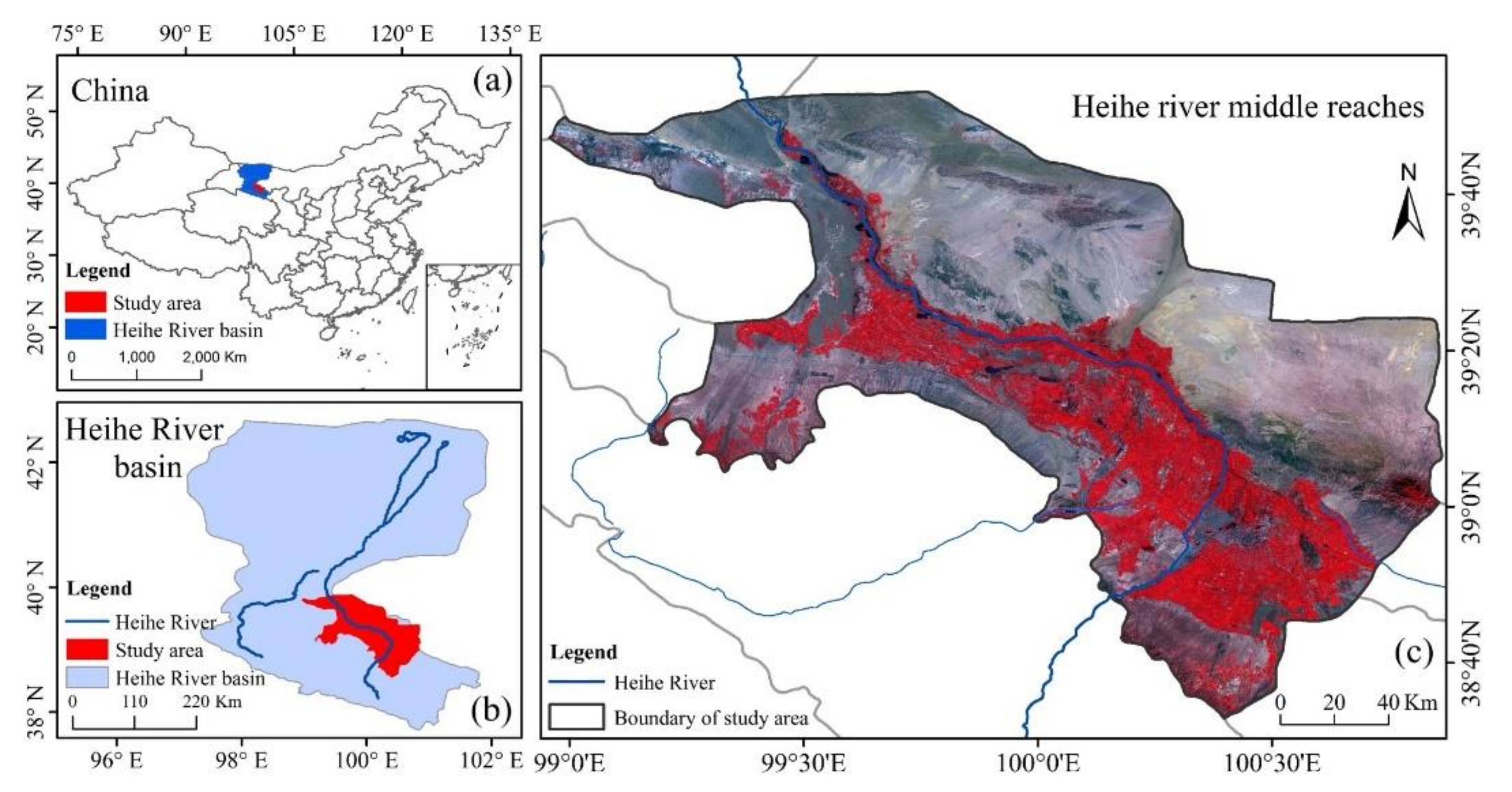
Figure 1. Study area of the middle reaches of Heihe River showing (a) location of the study area in China, (b) location of the study area in Heihe River basin, (c) Sentinel-2 composite image in August of false-color composite.
Remotesensing 13 02988 g001
Figure 2. Technical flow of the maize planting area extraction scheme. “k = k − 5” represents the elimination of 5 smallest importance features in each iteration process. It includes three parts: (1) Data preparation and preprocessing; (2) Extraction of vegetation area using S2 images; (3) Extraction of corn planting area using S1(alone), S2(alone) and combined dataset, respectively.
Remotesensing 13 02988 g002
Figure 3. The vegetation extraction result in the study area. “Yellow” represents the non-vegetation area, “purple” represents the vegetation area, and then the maize planting area will be further extracted in the vegetation area.
Remotesensing 13 02988 g003
Figure 4. The importance of 30 input indicators in vegetation extraction. Note that the values of importance of variables have been normalized. The change from blue to red indicates the increasing trend of the importance of variables.
Remotesensing 13 02988 g004
Figure 5. The feature indicators that used to construct three different RF maize extraction models of RF_S1, RF_S2, and RF_ S1&S2, respectively. (a) the 24 feature indicators from S1 (alone); (b) the 30 optimal feature indicators from S2 (alone); (c) the optimal 40 feature indicators from combined S1 and S2 data.
Remotesensing 13 02988 g005aRemotesensing 13 02988 g005b
Figure 6. (a) Distribution map of maize planting area in the study area; (b) The false color composite map of a local enlarged typical desert-oasis zone; and (c) maize distribution map of the typical zone.
Remotesensing 13 02988 g006
Figure 7. The number of good observations in the study area from April to September. Banded areas had a higher value due to the more S2 images are overlapped. The color in the graph represents the amount of data available on the pixel during the time interval. From “blue” to “red” indicates that the number of good observations increases gradually.
Remotesensing 13 02988 g007
Figure 8. Performance comparison of different RF models constructed by incremental learning and feature selection. “noFSP” means that the feature selection procedure is not used. In the figure, the month marked on the abscissa means that the input features of the RF model include the data of that month and previous months.
Remotesensing 13 02988 g008aRemotesensing 13 02988 g008b
Table 1. Bands and spectral indicators form Sentinel 1 and Sentinel 2 images.
Band or IndexCentral Wavelength/Index FormulaSatellite
1VV S1
2VH S1
3VV-VHVV-VHS1
4VV/VHVV/VHS1
5B1443.9 nm(S2A)/442.3 nm(S2B)S2
6B2496.6 nm(S2A)/492.1 nm(S2B)S2
7B3560 nm(S2A)/559 nm(S2B)S2
8B4664.5 nm(S2A)/665 nm(S2B)S2
9B5703.9 nm(S2A)/703.8 nm(S2B)S2
10B6740.2 nm(S2A)/739.1 nm(S2B)S2
11B7782.5 nm(S2A)/779.7 nm(S2B)S2
12B8835.1 nm(S2A)/833 nm(S2B)S2
13B8A864.8 nm(S2A)/864 nm(S2B) S2
14B9945 nm(S2A)/943.2 nm(S2B)S2
15B101373.5 nm(S2A)/1376.9 nm(S2B)S2
16B111613.7 nm(S2A)/1610.4 nm(S2B)S2
17B122202.4 nm(S2A)/2185.7 nm(S2B)S2
18NDVI(B8 − B4)/(B8 + B4)S2
19RDNDVI1(B8 − B5)/(B8 + B5)S2
20RDNDVI2(B8 − B6)/(B8 + B6)S2
21GCVI(B8/B3) − 1S2
22RDGCVI1(B8/B5) − 1S2
23RDGCVI2(B8/B6) − 1S2
24REIP700 + 40 × ((B4 + B7)/2 − B5)/(B7 − B5)S2
25NBR1(B8 − B11)/(B8 + B11)S2
26NBR2(B8 − B12)/(B8 + B12)S2
27NDTI(B11 − B12)/(B11 + B12)S2
28CRC(B11 − B3)/(B11 + B3)S2
29STIB11/B12S2
30NDBI(B12 − B4)/(B12 + B4)S2
31NDWI(B3 − B4)/(B3 + B4)S2
32LSWI(B4 − B11)/(B4 + B11)S2
33EVI2.5 × (B8 − B4)/(B8 + 6 × B4 − 7.5 × B2 + 1)S2
34REP705 + 35 × (0.5 × (B7 + B4) − B5)/(B6 − B5)S2
Table 2. The performance quantitative evaluation results of RF_S1, RF_S2 and RF_S1&S2 for training set and test set for using S1 (alone), S2 (alone) and combination of S1 and S2.
Confusion MatrixPredictive ValueRPOAKAPPAF1_Score
MaizeNon-Maize
actual value
(training set)
RF_S1
maize386680.840.8586.42%0.720.84
non-maize725050.880.88
RF_S2
maize404520.860.8988.39%0.760.87
non-maize685100.910.88
RF_S1&S2
maize412440.90.989.46%0.790.90
non-maize655130.890.89
actual value
(test set)
RF_S1
maize103240.760.8180.14%0.60.78
non-maize321230.840.79
RF_S2
maize110170.820.8785.51%0.710.84
non-maize241320.890.85
RF_S1&S2
maize113140.840.8987.63%0.750.86
non-maize211350.910.87
Table 3. Comparison of maize classification accuracy before and after S2 and S1 image pre-processing. Preprocessing refers to moving median synthesis for S2 images and 7 × 7 Refined Lee spectral filtering for S1 images.
S2-Moving Median ProcessingS1-7 × 7 Refined Lee Speckle Filter
monthOAKAPPAF1_ScoreOAKAPPAF1_Score
beforeafterbeforeafterbeforeafterbeforeafterbeforeafterbeforeafter
480.18%80.71%0.580.610.730.7869.26%71.68%0.340.410.590.64
579.77%79.46%0.590.590.760.7771.21%73.05%0.420.450.670.69
674.91%77.46%0.490.540.710.7469.89%69.06%0.400.380.680.68
Publisher’s Note: MDPI stays neutral with regard to jurisdictional claims in published maps and institutional affiliations.