Abstract
The Korea Meteorological Administration (KMA) has developed many product algorithms including that for soil moisture (SM) retrieval for the geostationary satellite Geo-Kompsat-2A (GK-2A) launched in December 2018. This was developed through a five-year research project owing to the significance of SM information for hydrological and meteorological applications. However, GK-2A’s visible and infrared sensors lack direct SM sensitivity. Therefore, in this study, we developed an SM algorithm based on the conversion relationships between SM and the temperature vegetation dryness index (TVDI) estimated for various land types in the full disk area using two of GK-2A’s level 2 products, land surface temperature (LST) and normalized difference vegetation index (NDVI), and the Global Land Data Assimilation System (GLDAS) SM data for calibration. Methodologically, various coefficients were obtained between TVDI and SM and used to estimate the GK-2A-based SM. The GK-2A SM algorithm was validated with GLDAS SM data during different periods. Our GK-2A SM product showed seasonal and spatial agreement with GLDAS SM data, indicating a dry-wet pattern variation. Quantitatively, the GK-2A SM showed annual validation results with a correlation coefficient (CC) >0.75, bias <0.1%, and root mean square error (RMSE) <4.2–4.7%. The monthly averaged CC values were higher than 0.7 in East Asia and 0.5 in Australia, whereas RMSE and unbiased RMSE values were <0.5% in East Asia and Australia. Discrepancies between GLDAS and GK-2A TVDI-based SMs often occurred in dry Australian regions during dry seasons due to the high LST sensitivity of GK-2A TVDI. We determined that relationships between TVDI and SM had positive or negative slopes depending on land cover types, which differs from the traditional negative slope observed between TVDI and SM. The KMA is currently operating this GK-2A SM algorithm.
1. Introduction
Soil moisture (SM) is a significant variable for understanding the hydrological cycle, agriculture, weather forecasting, and water management. Dry soil often provides favorable conditions for natural disasters such as wildfires and desertification [1,2,3], whereas wet soil information can be utilized for detecting floods or abnormal overflow of rivers. SM regulates the Earth’s thermal energy balance through interactions between the soil and the atmosphere [4,5,6,7,8,9]. SM is also considered a fundamental parameter in climate change studies and atmospheric circulation [9,10,11].
Although providing point measurements within limited regions, ground observations are the most accurate and commonly used to obtain land variable data such as SM. Satellite remote sensing presents the advantage of providing global SM observations including for regions lacking ground measurements. Thus, satellites equipped with the visible (VIS), infrared (IR), and microwave (MW) sensors have been mainly used to obtain SM information through remote sensing [12,13,14,15,16,17,18]. MW radiation tends to be well absorbed by water particles [19,20,21,22,23]. Thus, MW satellites have been mainly used for soil monitoring (depths of 0–10 cm) [24,25,26,27] with coarse temporal and spatial resolutions. However, SM products using MW satellites, including the National Aeronautics and Space Administration’s (NASA) Soil Moisture Active Passive (SMAP) and European Space Agency’s (ESA) Soil Moisture and Ocean Salinity (SMOS), have not shown good performance in the Korean Peninsula, where forested mountains cover 70% of the region. Recently, geostationary satellites using VIS and IR sensors with high temporal and spatial resolution have been used for SM research [28,29,30,31,32]. VIS/IR satellite remote sensing adopts indirect methods such as using the temperature vegetation dryness index (TVDI) based on the land surface temperature (LST) and the normalized difference vegetation index (NDVI) [33,34,35], because VIS and IR sensors cannot directly observe SM.
The Geo-Kompsat-2A (GK-2A) satellite is a geostationary weather satellite developed by the Korea Aerospace Research Institute (KARI) and National Meteorological Satellite Center (NMSC) of the Korea Meteorological Agency (KMA). It was launched on 5 December 2018, and it began operating on 25 July 2019. As a successor of the Communication, Ocean and Meteorological Satellite (COMS), it has an advanced meteorological imager (AMI) sensor with 16 bands [36]. GK-2A/AMI level (L) 1B products with a spatial resolution of 0.5–2 km and a temporal resolution of 10 min provide near real-time observations. The NMSC/KMA has developed various L2 and L3 products such as LST and NDVI using GK-2A/AMI L1B products [37,38] through a five-year research project for increasing the diversification of the AMI’s 16 channels. This study presents one GK-2A L3 product and SM products of GK-2A/AMI as part of the GK-2A/AMI algorithm development research project.
Physically, SM is particularly affected by LST and vegetation. For example, the NDVI value remains approximately constant because of the delayed response to SM, whereas LST changes immediately in response to water stress [39]. Additionally, the interaction between NDVI and LST determines the thermal capacity of the soil [34,39,40,41,42,43,44,45,46]. The relationship between NDVI and LST has been studied for a variety of meteorological variables such as evapotranspiration and air temperature [47,48,49]. The properties of slopes of the NDVI and LST relationships have been used in SM studies [39,43,50,51,52].
TVDI is an index developed to empirically interpret the water stress associated with surface temperature and vegetation within the NDVI/LST space [33,40,42]; this representative method uses slopes of NDVI and LST relationships. Recently, many studies have focused on the TVDI-based SM retrieval algorithm using VIS/IR bands because of their high spatial resolutions. The satellite-based TVDI was correlated negatively with ground-based SM observations [53]. Moran et al. [42] analyzed the relationship between the soil–vegetation–atmosphere transfer (SVAT) model and TVDI, and presented the concept of a water deficit index (WDI) related to the actual or potential evapotranspiration rate of surfaces, which describes how SM can be reproduced from the partial vegetation cover of NDVI/LST spaces using the SVAT models. Moran et al. [54] validated the NDVI/LST method through simulations. Areas with sparse canopy may be less related to SM than are moist surfaces as the satellite-derived surface temperature is affected by vegetation and soil surfaces [55].
This study presents the GK-2A SM retrieval algorithm using TVDI and GK-2A/AMI products. The GK-2A SM was estimated using the conversion relationships between the Global Land Data Assimilation System (GLDAS) SM and TVDI calculated using the GK-2A LST and NDVI products for various land cover types [30,56,57] in the daily full disk area of the GK-2A, because the use of GLDAS SM was a KMA requirement for SM algorithm development and validation. The GK-2A SM was temporally and spatially compared with the GLDAS SM for different periods. In addition, this study confirmed the dependence of TVDI characteristics on land cover type.
2. Study Area and Data
2.1. Study Area
The study area included the entire GK-2A disk area, including Australia in the southern hemisphere and East Asia and the Korean Peninsula in the northern hemisphere, as observed by GK-2A located at 128.0° E. The data from August 2019 to July 2020 were utilized because the GK-2A began to operate on 25 July 2019 [36]. The verification of the calculated GK-2A soil moisture was carried out on a different date from the one on which the soil moisture conversion coefficient was calculated. The ocean pixels in the full disk data were masked using the land/sea mask data of GK-2A. The pixels with the solar zenith angle of 70° or higher were also masked due to inaccurate satellite observation. In addition, the water, permanent wet land, urban, built-up, snow, and ice regions were excluded using the GK-2A land cover data. Figure 1 shows the study area for estimating TVDI and soil moisture. For validation, we cropped East Asia to represent the northern hemisphere and Australia to represent the southern hemisphere from the full disk.
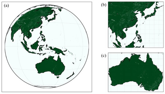
Figure 1.
(a) Study area used for obtaining soil moisture coefficients. Validation areas of (b) East Asia and (c) Australia.
2.2. GK-2A/AMI Satellite
The GK-2A satellite, located at 128.0° E, covers East Asia, including the Korea peninsula, and Australia in the full disk every 10 min. The GK-2A/AMI sensor has 16 VIS and IR channels. A variety of GK-2A L2 products such as the LST and NDVI have been developed [37,38,58]. In this study, we used the GK-2A LST and NDVI L2 products for estimating the TVDI, and GLDAS SM data, which were provided by NMSC/KMA. Table 1 summarizes the full disk data information used in this study.

Table 1.
Input and ancillary data for the GK-2A TVDI calculation.
Table 2 summarizes the land covers used in this study. Notably, land cover areas were fixed because of annual average values. This may have caused differences around the borders between two different land types.

Table 2.
GK-2A land cover types.
2.3. GLDAS
GLDAS, including SM, soil condition, and canopy condition data [59], is one of the representative global modeling systems for the land environment provided by NASA. It has been available since 1948. GLDAS SM data have been widely used as verification data in various SM studies [5,60,61,62]. The GLDAS products incorporate various modeling systems (Noah, CLM, VIC, and Mosaic) and various datasets based on ground observations. GLDAS has a spatial resolution of 0.25° and 1.0°, and a temporal resolution of 3 h and 1 month for monitoring daily and monthly variations. In particular, GLDAS SM data include many soil layers: 0–10 cm, 10–40 cm, 40–100 cm, and 100–200 cm.
This study used the GLDAS L4 SM data for the 0–10 cm layer with a 0.25° spatial resolution and a 3 h temporal resolution for the development and validation of the GK-2A SM algorithm according to the KMA’s requirements for algorithm development.
3. Methods
3.1. TVDI Calculation Using GK-2A LST and NDVI
In this study, TVDI is an intermediate parameter used to estimate the GK-2A SM. TVDI is determined in the LST/NDVI space as a function of and , which are obtained from the linear regressions of NDVI and LST [40,42]. Figure 2 shows a scatterplot between the NDVI and the LST and illustrates the characteristics of TVDI. The regression line with the top dashed line represents , and the regression line with the bottom dashed line indicates . represents the dry edge, while indicates the wet edge. In the dry edge, the TVDI value is 1, which mainly exists in the bare soil and savanna. In the wet edge, the TVDI value is 0, which mostly occurs in forests and vegetation canopies.
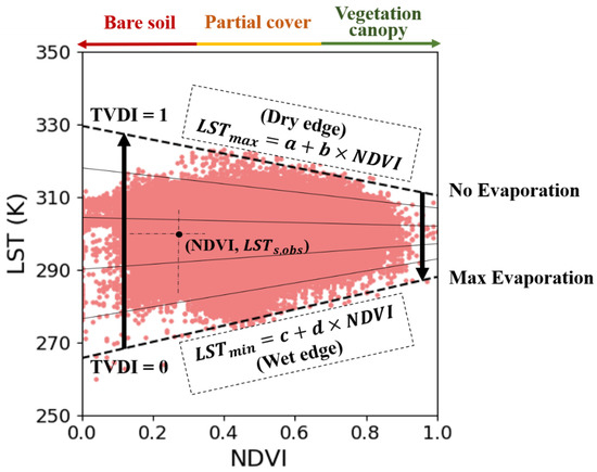
Figure 2.
Example of a TVDI distribution and its characteristics in NDVI/LST space.
Two edge lines and in the LST/NDVI space are expressed as follows [33,40,42]:
where , b, c, d are the coefficients determined for and using real LST and NDVI data. This study used the GK-2A L2 LST and NDVI products. Table 3 shows the coefficient values of and according to the land cover on 19 July 2020.

Table 3.
Coefficients of and .
TVDI is calculated using and as follows:
where is the observed LST at a specific pixel.
3.2. Conversion Relationship between TVDI and SM
In this study, we applied linear regression to convert TVDI into SM based on the existent linear relationships between TVDI and model SM [63] as follows:
where SM is the GK-2A SM in units of volumetric ratio (). A and B are the intercept and the slope for converting TVDI into SM, respectively.
In this step, we used the GLDAS SM and GK-2A–derived TVDI to obtain these slopes and intercepts for various land cover types.
Table 4 summarizes the data periods in which we obtained the conversion coefficients between TVDI and SM and validated the GK-2A–derived SM.

Table 4.
Data periods for calibration and validation of GK-2A-derived SM.
Table 5 summarizes the daily-averaged slopes and intercepts for different land cover types in the northern and southern hemispheres on 9 July 2020. Our linear relationships between TVDI and GLDAS SM for 16 land types showed low correlation coefficient values ranging from −0.432 to 0.268 in the northern hemisphere, while we found high correlation coefficients ranging from −0.845 to 0.360 in the southern hemisphere. In particular, our study showed a relatively low correlation between TVDI and SM for forests and savannas in the northern hemisphere and showed variable correlations, including high correlations for open shrublands, savannas, and grasslands and low correlations for mixed forest and closed shrublands, in the southern hemisphere. Notably Chen et al. (2015) [53] showed a negative correlation between the TVDI using LANDSAT-5 Thematic Mapper data and the in situ measured SM (R2 = 0.15–0.8 in the Laoshan forest, the largest forest in Nanjing, China) under different tree species.

Table 5.
Conversion coefficients and their statistics (R, p-value, RMSE) for TVDI and SM for 16 land cover types on 19 July 2020.
In this study, all the data were synthesized as 10-day average data as per another requirement of the NMSC/KMA for their use. Notably, the elevation-correction to the LST was not performed because the GK-2A LST data were already calibrated according to the elevation pressure [37,58]. The GK-2A and GLDAS collocated in terms of their respective latitude and longitude data based on the calculation of the latitude and longitude of the nearest distance. Figure 3 shows a flowchart of the GK-2A TVDI-based SM algorithm.
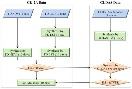
Figure 3.
Flow chart of the GK-2A TVDI-based SM retrieval algorithm.
3.3. Statistical Factors
In this study, the GK-2A SMs were quantitatively validated with the GLDAS SM data using the statistical indices: correlation coefficient (CC), bias, the root mean square error (RMSE), and unbiased RMSE (ubRMSE) as follows [64,65]:
where is the total number of pixels in the corresponding GK-2A and GLDAS data, is the index from 1 to N, indicates the SM of the pixel in the GLDAS data, and indicates the SM of the pixel in the GK-2A data. and are the mean values of the GLDAS and GK-2A SM data, respectively.
4. Results
4.1. TVDI
Figure 4 shows the scatterplots between NDVI and LST data of GK-2A for 13 different land cover types (evergreen needleleaf forest, evergreen broadleaf forest, deciduous needleleaf forest, deciduous broadleaf forest, mixed forest, closed shrublands, open shrublands, woody savannas, savannas, grasslands, croplands, cropland/natural vegetation mosaic, and barren or sparsely vegetated) in the northern hemisphere on 19 July 2020. The top and bottom dashed lines indicate the linear regression lines of the maximum and minimum LST values, respectively.
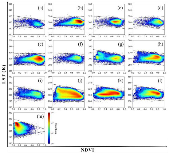
Figure 4.
Scatterplots of NDVI and LST on 19 July 2020 for 13 land cover types: (a) Evergreen Needleleaf Forest, (b) Evergreen Broadleaf Forest, (c) Deciduous Needleleaf Forest, (d) Deciduous Broadleaf Forest, (e) Mixed Forest, (f) Closed Shrublands, (g) Open Shrublands, (h) Woody Savannas, (i) Savannas, (j) Grasslands, (k) Croplands, (l) Cropland/Natural Vegetation Mosaic, and (m) Barren or Sparsely Vegetated.
Figure 5 illustrates the spatial distributions of land cover, 10-day averaged GK-2A LST, NDVI, and the estimated TVDI values on 19 July 2020 (summer in the northern hemisphere and winter in the southern hemisphere). The LST values were high in the Gobi Desert in summer and northern Australia in winter. The NDVI values showed in the typical distribution. The TVDI values were high in the desert areas, southeastern Asia, tropical regions, and northern Australia, and low in Tibet, Siberia, southern Australia, and New Zealand.
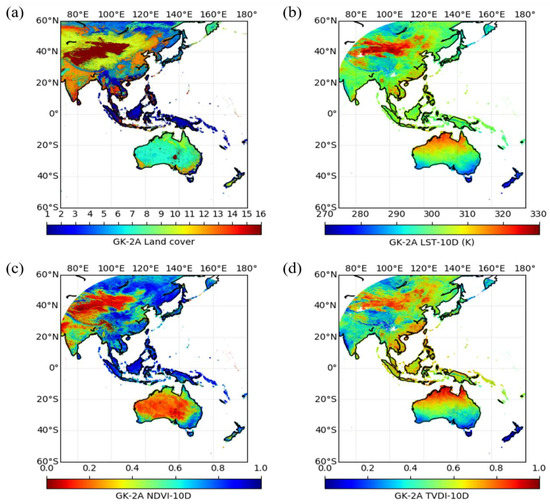
Figure 5.
Spatial distributions of GK-2A (a) land cover and 10-day averaged (b) LST, (c) NDVI, and (d) TVDI on 19 July 2020.
Figure 6 shows the temporal variation of the 10-day averaged slopes of for various land types in East Asia and Australia during winter, spring, summer, and autumn of one year [55]. Sandholt et al. (2002) [55] reported that the slope of the function in the NDVI/LST space can be an indicator for determining dry periods [55]; further, TVDI is particularly variable in dry regions or dry periods as compared to those in wet regions or periods [55].
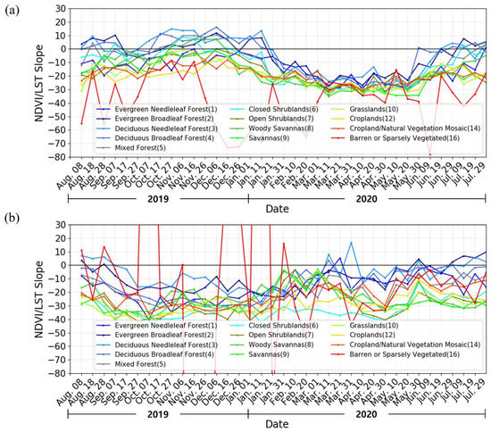
Figure 6.
Time series of the slopes of the NDVI/LST space in (a) East Asia and (b) Australia from August 2019 to July 2020.
The slopes for both East Asia and Australia showed common sinusoidal seasonal variations, which decreased relatively quickly during the dry season, from winter to early summer, and increased during other seasons. The slope values fluctuated more severely during the dry period from winter to early summer than during the wet period from summer to early winter. Notably, the barren or sparsely vegetated area (land cover 16) showed the highest variation in the slope value. Furthermore, the comparison between East Asia and Australia showed increased slope variation for each land cover in Australia compared to those in East Asia due to the higher ratio of dry regions in Australia than those in East Asia. These results show agreement with those of a previous study [55].
Figure 7 illustrates the 10-day-averaged TVDI values for various land cover types in East Asia and Australia. Notably, the amount of vegetation decreased and the heights of trees decreased as the amount of land cover increased. East Asia showed stable temporal variations in TVDI values in general land types except for bare soil in spring. Australia showed similar patterns to East Asia, and greater variation for bare soil (land cover 16) than in East Asia. We identified that TVDI values highly fluctuated during the dry periods from January 1 to May 10 in East Asia and from August 28 to May 1 in Australia. The TVDI values were sometimes >1, especially in Australia, which is in agreement with a previous finding that TVDI values often exceed 1 in regions where LST is rapidly increasing because TVDI is sensitive to the effects of LST [55]. Thus, we examined the distributions of LST in East Asia and Australia during winter and summer (Figure 8) because TVDI values varied more in Australia than they did in East Asia and were often >1.
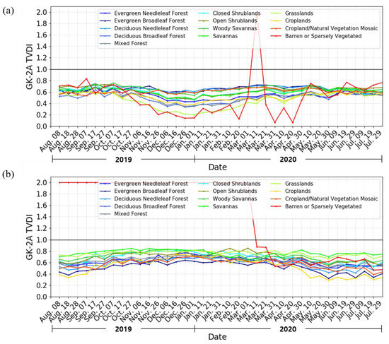
Figure 7.
Temporal distributions of the averaged TVDI for each date and land cover in (a) East Asia and (b) Australia from August 2019 to July 2020.
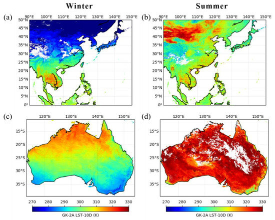
Figure 8.
GK-2A LST distributions in East Asia on (a) 11 January 2020 (winter) and (b) 19 July 2020 (summer) and in Australia on (c) 19 July 2020 (winter) and (d) 11 January 2020 (summer).
Figure 8 shows the high sensitivity of TVDI values to LST values in East Asia and Australia, and supports the analysis presented in Figure 7. The LST values in Australia increased sharply because most regions in Australia were dry except for the outskirts. In addition, LST increased rapidly in the Gobi Desert compared to that in other regions in East Asia. Therefore, TVDI values are often >1.
4.2. GK-2A SM
Figure 9 shows the three-month-averaged GK-2A and GLDAS SM data for spring (March, April, and May), summer (June, July, and August), autumn (September, October, and November), and winter (December, January, and February). The GK-2A SM showed a similar pattern to that of GLDAS SM including dry-wet patterns, while GK-2A SM showed discontinuous SM patterns near the Gobi Desert in the northern hemisphere and inland Australia in the southern hemisphere due to the fixed land cover area.
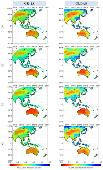
Figure 9.
Spatial distribution of GK-2A and GLDAS SM during four seasons: (a) spring (March, April, May), (b) summer (June, July, August), (c) autumn (September, October, November), and (d) winter (December, January, February).
Figure 10 shows the results of the statistical comparison between the GLDAS and GK-2A SM shown in Figure 9. The CC ranged from 0.767 to 0.846. The bias ranged from −0.001 to 0.001 . The RMSE ranged from 0.042 to 0.047 . These results indicated that the estimated GK-2A SM shows good agreement with GLDAS SM. Notably, the accuracy requirement of SM for MW satellite remote sensing, such as the NASA SMAP SM product, is 4% (0.04 ) in the top 5 cm of soil at a 40 km spatial resolution and 3-day-average intervals over the global land area excluding regions of snow and ice, frozen ground, mountainous topography, open water, and urban areas (https://smap.jpl.nasa.gov/science/objectives, access on 11 May 2021) Further, the RMSE of our GK-2A SM results ranged within the analogous values of the error requirement of SMAP SM. Table 6 summarizes the statistical results of the previous scatterplots.
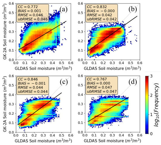
Figure 10.
Scatterplots between GLDAS and GK-2A SM for the four seasons of (a) spring, (b) summer, (c) autumn, and (d) winter.

Table 6.
Statistical comparison results between GLDAS and GK-2A SM.
Figure 11 shows the temporal variation of GK-2A SM for different land types in East Asia and Australia. In both hemispheres, GK-2A SM showed similar patterns of variation. In general, land cover types from 1 to 5 corresponding to forests showed relatively high SM values of approximately 0.3 , whereas land cover 16 (bare soil region) showed the lowest seasonal variation of SM values from 0.1 in winter and 0.15 in summer in East Asia and from 0.1 to 0.2 in Australia. In East Asia, the average SM values ranged between 0.2 and 0.3 , whereas they varied from 0.1 to 0.3 in Australia. This result may be attributed to the relatively higher ratio of dry regions in the southern hemisphere compared to that in the northern hemisphere.
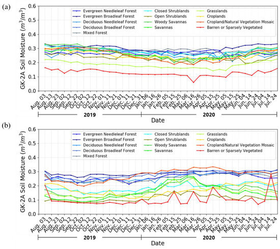
Figure 11.
Temporal variations in the 10-day-averaged GK-2A SM for each land cover type in (a) East Asia and (b) Australia from August 2019 to July 2020.
Figure 12 shows the different characteristics of GK-2A SM in the northern and southern hemispheres based on the temporal dynamics of the spatial CC and RMSE between GK-2A and GLDAS SM in East Asia and Australia during one year. Figure 12a shows good and consistent agreement of CC (>0.7) between GK-2A and GLDAS SM in East Asia. In Australia, the CC values from February to November were similar to those in East Asia, whereas the CC values decreased rapidly during January and December, i.e., summer in the southern hemisphere. This may be attributed to the rapid increase of the LST effect in the Australian summer, which was described with the TVDI values being >1 in this period. Notably, Figure 12b,c shows that RMSE and ubRMSE values in Australia were consistent and smaller (0.03 to 0.04 ) than those in East Asia (0.04 to 0.05 ). However, the CC values dropped in January and December, which is summer in the southern hemisphere.
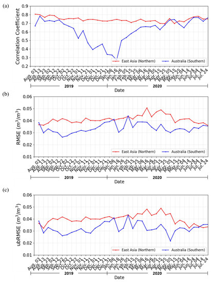
Figure 12.
Temporal dynamics of the spatial (a) CC, (b) RMSE, and (c) ubRMSE between the 10-day-averaged GLDAS and GK-2A SM in East Asia and Australia from August 2019 to July 2020.
5. Discussion
In this study, the conversion coefficients between TVDI and SM were obtained for each land cover. Previous TVDI studies indicated that TVDI was negatively correlated with the model and ground observations of SM. However, this study determined the existence of positive as well as negative correlations between TVDI and SM based on satellite observations and GLDAS SM data. TVDI variations in dry regions and periods increased due to the slope of , a function of NDVI and LST, which can undergo drastic changes [55].
Figure 13 shows the scatterplots with negative (Figure 13a,c) and positive slopes (Figure 13b,d) between TVDI and the SM for different land cover types from August 2019 to July 2020 in the full disk of the GK-2A. The results in Figure 13a,c showed agreement with previous studies [53,55], but Figure 13b,d indicated differing results. In terms of data frequency, different land cover types showed similar data pixels in the northern hemisphere, as shown in Figure 13a,b. However, data frequencies in the southern hemisphere were concentrated in small areas with high TVDI and low SM values in the TVDI and SM space, as shown in Figure 13c,d. These results indicate the simple land types such as dry regions in most parts of Australia.
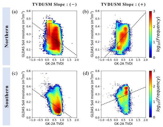
Figure 13.
Scatterplots between GK-2A TVDI and GLDAS SM from August 2019 to July 2020 with (a) negative and (b) positive slopes in the northern hemisphere, and (c) negative and (d) positive slopes in the southern hemisphere.
Figure 14 shows the positively correlated data distribution between TVDI and SM (Figure 13) represented in the NDVI/LST space. In Figure 14, the green line shows wet soil regions with high vegetation, high LST, and high TVDI values. The red line indicates dry soil regions with low vegetation, low LST, and high TVDI values. The regions with high vegetation density and high LST values were related to wet soil due to a high vegetation canopy. Thus, high TVDI values can be calculated based on the high LST value in this region. The regions with low vegetation density and low LST were related to dry soil due to a low vegetation canopy. However, high TVDI can be calculated based on the low LST value in this region.
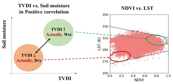
Figure 14.
Positively correlated distributions in the NDVI/LST space of TVDI.
The quality of microwave satellite-based SM values such as SMAP and SMOS is insufficient for surface conditions that include mountainous terrain and dense vegetation with high vegetation water content (VWC) [66] because of the dependence on the radiative transfer model; sensitivity of polarization to the surface SM; various and a priori ancillary data including physical temperature, vegetation, roughness, and soil texture [21]; or a relation between SM and VWC [12]. In particular, it is difficult to directly measure the VWC, while NDVI has a high sensitivity to abrupt environmental change, such as floods and droughts, without a priori information [67]. Thus, this study, based on the TVDI as a function of NDVI and LST, showed feasible results for the vegetated and mountainous topology in the Korean Peninsula in addition to providing SM information, including regions lacking ground measurements and SMAP and SMOS SM values, and supplementing low spatial and temporal resolutions of GLDAS SM in the Korean Peninsula.
6. Summary and Conclusions
This study presented the GK-2A SM algorithm using TVDI as a function of GK-2A LST and NDVI products. GLDAS SM data were used for GK-2A SM algorithm development and validation as a requirement of the KMA. We obtained the daily LST, NDVI, TVDI, and GLDAS SM data and then composited 10-day-averaged LST, NDVI, TVDI, and SM data for various land types. The conversion coefficients between TVDI and GLDAS SM for different land types were obtained and validated with GLDAS SM for different periods from August 2019 to July 2020. The results showed a high CC of >0.75 in East Asia and >0.5 in Australia for all seasons, low bias from −0.001 to 0.001 , and low RMSE of <0.05 . Notably, the RMSE results showed a low error rate of 0.05 or less, which is close to the NASA’s accuracy requirement for SM products for the SMAP mission. The GK-2A SM values were accurate except those for summer in Australia. The slope of , a function of NDVI and LST, can show drastic changes. Our results presented this characteristic in the drier southern hemisphere but not in the northern hemisphere. We also identified and explained the positive correlation between TVDI and SM due to the high sensitivity of TVDI to LST. Our GK-2A SM algorithm has an advantage of better spatial and temporal resolutions compared to those of the other algorithms implemented in geostationary weather satellites. It allows for the monitoring of more spatial structures that would not be identified by GLDAS, captures extreme events where the SM content can change very quickly, and shows an accuracy similar to that of SM products of polar-orbiting microwave satellites. However, the algorithm is dependent on the accuracy of GK-2A LST and NDVI products. The KMA is currently operating the proposed SM retrieval algorithm. A future scope of study will be to improve the conversion coefficients between TVDI and SM in our algorithm using the long-term GK-2A observational data.
Author Contributions
Conceptualization, S.H.; methodology, S.H., Y.-J.K. and S.R.; software, S.R.; validation, S.R. and S.H.; formal analysis, S.H. and S.R.; investigation, S.R., Y.-J.K. and S.H.; resources, S.H.; data curation, S.R. and G.K.; writing—original draft preparation, S.H. and S.R.; writing—review and editing, S.H.; visualization, S.R.; supervision, S.H.; project administration, G.K. and S.H.; funding acquisition, S.H. All authors have read and agreed to the published version of the manuscript.
Funding
This work was funded and supported by (1) “Development of Scene Analysis and Surface Algorithms” project, funded by ETRI, which is a subproject of the “Development of Geostationary Meteorological Satellite Ground Segment (NMSC-2019-01)” program funded by the NMSC (National Meteorological Satellite Center) of the Korea Meteorological Administration (KMA), (2) the KMA Research and Development Program under Grants KMI2020-00510, and (3) a grant from the National Institute of Environment Research (NIER), funded by the Ministry of Environment (MOE) of the Republic of Korea (NIER-2021-01-02-068).
Acknowledgments
The authors thank the anonymous reviewers for helpful and constructive comments on the manuscript.
Conflicts of Interest
The authors declare no conflict of interest.
References
- Li, S.; Ren, H.; Xue, L.; Chang, J.; Yao, X. Influence of bare rocks on surrounding soil moisture in the karst rocky desertification regions under drought conditions. Catena 2014, 116, 157–162. [Google Scholar] [CrossRef]
- Le Houérou, H.N. Climate change, drought and desertification. J. Arid Environ. 1996, 34, 133–185. [Google Scholar] [CrossRef]
- Gudmundsson, L.; Rego, F.C.; Rocha, M.; Seneviratne, S.I. Predicting above normal wildfire activity in southern Europe as a function of meteorological drought. Environ. Res. Lett. 2014, 9, 084008. [Google Scholar] [CrossRef]
- Ni-Meister, W. Recent advances on soil moisture data assimilation. Phys. Geogr. 2008, 29, 19–37. [Google Scholar] [CrossRef]
- Bi, H.; Ma, J.; Zheng, W.; Zeng, J. Comparison of soil moisture in GLDAS model simulations and in situ observations over the Tibetan Plateau. J. Geophys. Res. Atmos. 2016, 121, 2658–2678. [Google Scholar] [CrossRef]
- Monteith, J. Evaporation and surface temperature. Q. J. R. Meteorol. Soc. 1981, 107, 1–27. [Google Scholar] [CrossRef]
- Entekhabi, D. Recent advances in land-atmosphere interaction research. Rev. Geophys. 1995, 33, 995–1003. [Google Scholar] [CrossRef]
- Cahill, A.T.; Parlange, M.B.; Jackson, T.J.; O’Neill, P.; Schmugge, T. Evaporation from nonvegetated surfaces: Surface aridity methods and passive microwave remote sensing. J. Appl. Meteorol. 1999, 38, 1346–1351. [Google Scholar] [CrossRef][Green Version]
- Dirmeyer, P.A. Using a global soil wetness dataset to improve seasonal climate simulation. J. Clim. 2000, 13, 2900–2922. [Google Scholar] [CrossRef]
- Douville, H.; Chauvin, F. Relevance of soil moisture for seasonal climate predictions: A preliminary study. Clim. Dyn. 2000, 16, 719–736. [Google Scholar] [CrossRef]
- Drusch, M. Initializing numerical weather prediction models with satellite-derived surface soil moisture: Data assimilation experiments with ECMWF’s Integrated Forecast System and the TMI soil moisture data set. J. Geophys. Res. 2007, 112. [Google Scholar] [CrossRef]
- Njoku, E.G.; Jackson, T.J.; Lakshmi, V.; Chan, T.K.; Nghiem, S.V. Soil moisture retrieval from AMSR-E. IEEE Trans. Geosci. Remote Sens. 2003, 41, 215–229. [Google Scholar] [CrossRef]
- Kerr, Y.H.; Waldteufel, P.; Wigneron, J.-P.; Martinuzzi, J.; Font, J.; Berger, M. Soil moisture retrieval from space: The Soil Moisture and Ocean Salinity (SMOS) mission. IEEE Trans. Geosci. Remote Sens. 2001, 39, 1729–1735. [Google Scholar] [CrossRef]
- Barrett, B.W.; Dwyer, E.; Whelan, P. Soil moisture retrieval from active spaceborne microwave observations: An evaluation of current techniques. Remote Sens. 2009, 1, 210–242. [Google Scholar] [CrossRef]
- Verstraeten, W.W.; Veroustraete, F.; van der Sande, C.J.; Grootaers, I.; Feyen, J. Soil moisture retrieval using thermal inertia, determined with visible and thermal spaceborne data, validated for European forests. Remote Sens. Environ. 2006, 101, 299–314. [Google Scholar] [CrossRef]
- Yin, J.; Zhan, X.; Liu, J.; Moradkhani, H.; Fang, L.; Walker, J.P. Near-real-time one-kilometre Soil Moisture Active Passive soil moisture data product. Hydrol. Process. 2020, 34, 4083–4096. [Google Scholar] [CrossRef]
- Yang, K.; Chen, Y.; He, J.; Zhao, L.; Lu, H.; Qin, J.; Zheng, D.; Li, X. Development of a daily soil moisture product for the period of 2002–2011 in Chinese mainland. Sci. China Earth Sci. 2020, 63, 1113–1125. [Google Scholar] [CrossRef]
- Abbaszadeh, P.; Moradkhani, H.; Gavahi, K.; Kumar, S.; Hain, C.; Zhan, X.; Duan, Q.; Peters-Lidard, C.; Karimiziarani, S. High-Resolution SMAP Satellite Soil Moisture Product: Exploring the Opportunities. Bull. Am. Meteorol. Soc. 2021, 102, 309–315. [Google Scholar] [CrossRef]
- Wang, J.R.; Schmugge, T.J. An empirical model for the complex dielectric permittivity of soils as a function of water content. IEEE Trans. Geosci. Remote Sens. 1980, 18, 288–295. [Google Scholar] [CrossRef]
- Dobson, M.C.; Ulaby, F.T.; Hallikainen, M.T.; El-Rayes, M.A. Microwave dielectric behavior of wet soil-Part II: Dielectric mixing models. IEEE Trans. Geosci. Remote Sens. 1985, 23, 35–46. [Google Scholar] [CrossRef]
- Jackson, T.J. III. Measuring surface soil moisture using passive microwave remote sensing. Hydrol. Process 1993, 7, 139–152. [Google Scholar] [CrossRef]
- De Jeu, R.A.; Wagner, W.; Holmes, T.; Dolman, A.; Van De Giesen, N.; Friesen, J. Global soil moisture patterns observed by space borne microwave radiometers and scatterometers. Surv. Geophys. 2008, 29, 399–420. [Google Scholar] [CrossRef]
- Hong, S.; Shin, I. A physically-based inversion algorithm for retrieving soil moisture in passive microwave remote sensing. J. Hydrol. 2011, 405, 24–30. [Google Scholar] [CrossRef]
- Ellingson, S.W.; Johnson, J.T. A polarimetric survey of radio-frequency interference in C-and X-bands in the continental United States using WindSat radiometry. IEEE Trans. Geosci. Remote Sens. 2006, 44, 540–548. [Google Scholar] [CrossRef]
- Li, L.; Njoku, E.G.; Im, E.; Chang, P.S.; Germain, K.S. A preliminary survey of radio-frequency interference over the US in Aqua AMSR-E data. IEEE Trans. Geosci. Remote Sens. 2004, 42, 380–390. [Google Scholar] [CrossRef]
- Njoku, E.G.; Entekhabi, D. Passive microwave remote sensing of soil moisture. J. Hydrol. 1996, 184, 101–129. [Google Scholar] [CrossRef]
- Newton, R.W.; Black, Q.R.; Makanvand, S.; Blanchard, A.J.; Jean, B.R. Soil moisture information and thermal microwave emission. IEEE Trans. Geosci. Remote Sens. 1982, GE-20, 275–281. [Google Scholar] [CrossRef]
- Bowers, S.A.; Hanks, R. Reflection of radiant energy from soils. Ph.D. Thesis, Kansas State University, Manhattan, NY, USA, 1971. [Google Scholar]
- Price, J.C. Thermal inertia mapping: A new view of the earth. J. Geophys. Res. 1977, 82, 2582–2590. [Google Scholar] [CrossRef]
- Stoner, E.R.; Baumgardner, M. Characteristic variations in reflectance of surface soils. Soil Sci. Soc. Am. J. 1981, 45, 1161–1165. [Google Scholar] [CrossRef]
- Lobell, D.B.; Asner, G.P. Moisture effects on soil reflectance. Soil Sci. Soc. Am. J. 2002, 66, 722–727. [Google Scholar] [CrossRef]
- Liu, W.; Baret, F.; Gu, X.; Zhang, B.; Tong, Q.; Zheng, L. Evaluation of methods for soil surface moisture estimation from reflectance data. Int. J. Remote Sens. 2003, 24, 2069–2083. [Google Scholar] [CrossRef]
- Price, J.C. Using spatial context in satellite data to infer regional scale evapotranspiration. IEEE Trans. Geosci. Remote Sens. 1990, 28, 940–948. [Google Scholar] [CrossRef]
- Gillies, R.; Kustas, W.; Humes, K. A verification of the ‘triangle’ method for obtaining surface soil water content and energy fluxes from remote measurements of the Normalized Difference Vegetation Index (NDVI) and surface e. Int. J. Remote Sens. 1997, 18, 3145–3166. [Google Scholar] [CrossRef]
- Kwon, Y.-J.; Ryu, S.; Cho, J.; Lee, Y.-W.; Park, N.-W.; Chung, C.-Y.; Hong, S. Infrared Soil Moisture Retrieval Algorithm Using Temperature-Vegetation Dryness Index and Moderate Resolution Imaging Spectroradiometer Data. Asia Pac. J. Atmos. Sci. 2020, 56, 275–289. [Google Scholar] [CrossRef]
- Chung, S.-R.; Ahn, M.-H.; Han, K.-S.; Lee, K.-T.; Shin, D.-B. Meteorological Products of Geo-KOMPSAT 2A (GK2A) Satellite. Asia Pac. J. Atmos. Sci. 2020, 56, 185. [Google Scholar] [CrossRef]
- Choi, Y.-Y.; Suh, M.-S. Development of a Land Surface Temperature Retrieval Algorithm from GK2A/AMI. Remote Sens. 2020, 12, 3050. [Google Scholar] [CrossRef]
- Seong, N.; Han, K.-S.; Lee, K.; Seo, M. Estimation NDVI using normalized reflectance through GK-2A/AMI data. In Proceedings of the AGU Fall Meeting Abstracts, AGU, San Francisco, CA, USA, 13 December 2019. [Google Scholar]
- Goetz, S. Multi-sensor analysis of NDVI, surface temperature and biophysical variables at a mixed grassland site. Int. J. Remote Sens. 1997, 18, 71–94. [Google Scholar] [CrossRef]
- Carlson, T.N.; Gillies, R.R.; Perry, E.M. A method to make use of thermal infrared temperature and NDVI measurements to infer surface soil water content and fractional vegetation cover. Remote Sens. Rev. 1994, 9, 161–173. [Google Scholar] [CrossRef]
- Clarke, T.R. An empirical approach for detecting crop water stress using multispectral airborne sensors. Horttechnology 1997, 7, 9–16. [Google Scholar] [CrossRef]
- Moran, M.; Clarke, T.; Inoue, Y.; Vidal, A. Estimating crop water deficit using the relation between surface-air temperature and spectral vegetation index. Remote Sens. Environ. 1994, 49, 246–263. [Google Scholar] [CrossRef]
- Nemani, R.R.; Running, S.W. Estimation of regional surface resistance to evapotranspiration from NDVI and thermal-IR AVHRR data. J. Appl. Meteorol. Climatol. 1989, 28, 276–284. [Google Scholar] [CrossRef]
- Lambin, E.F.; Ehrlich, D. The surface temperature-vegetation index space for land cover and land-cover change analysis. Int. J. Remote Sens. 1996, 17, 463–487. [Google Scholar] [CrossRef]
- Nemani, R.; Pierce, L.; Running, S.; Goward, S. Developing satellite-derived estimates of surface moisture status. J. Appl. Meteorol. Climatol. 1993, 32, 548–557. [Google Scholar] [CrossRef]
- Nemani, R.; Running, S. Land cover characterization using multitemporal red, near-IR, and thermal-IR data from NOAA/AVHRR. Ecol. Appl. 1997, 7, 79–90. [Google Scholar] [CrossRef]
- Boegh, E.; Soegaard, H.; Hanan, N.; Kabat, P.; Lesch, L. A remote sensing study of the NDVI–Ts relationship and the transpiration from sparse vegetation in the Sahel based on high-resolution satellite data. Remote Sens. Environ. 1999, 69, 224–240. [Google Scholar] [CrossRef]
- Prihodko, L.; Goward, S.N. Estimation of air temperature from remotely sensed surface observations. Remote Sens. Environ. 1997, 60, 335–346. [Google Scholar] [CrossRef]
- Son, N.T.; Chen, C.; Chen, C.; Chang, L.; Minh, V.Q. Monitoring agricultural drought in the Lower Mekong Basin using MODIS NDVI and land surface temperature data. Int. J. Appl. Earth Obs. Geoinf. 2012, 18, 417–427. [Google Scholar] [CrossRef]
- Friedl, M.; Davis, F. Sources of variation in radiometric surface temperature over a tallgrass prairie. Remote Sens. Environ. 1994, 48, 1–17. [Google Scholar] [CrossRef]
- Smith, R.; Choudhury, B. Analysis of normalized difference and surface temperature observations over southeastern Australia. Remote Sens. 1991, 12, 2021–2044. [Google Scholar] [CrossRef]
- Goward, S.N.; Xue, Y.; Czajkowski, K.P. Evaluating land surface moisture conditions from the remotely sensed temperature/vegetation index measurements: An exploration with the simplified simple biosphere model. Remote Sens. Environ. 2002, 79, 225–242. [Google Scholar] [CrossRef]
- Chen, S.; Wen, Z.; Jiang, H.; Zhao, Q.; Zhang, X.; Chen, Y. Temperature vegetation dryness index estimation of soil moisture under different tree species. Sustainability 2015, 7, 11401–11417. [Google Scholar] [CrossRef]
- Moran, M.; Clarke, T.; Kustas, W.; Weltz, M.; Amer, S. Evaluation of hydrologic parameters in a semiarid rangeland using remotely sensed spectral data. Water Resour. Res. 1994, 30, 1287–1297. [Google Scholar] [CrossRef]
- Sandholt, I.; Rasmussen, K.; Andersen, J. A simple interpretation of the surface temperature/vegetation index space for assessment of surface moisture status. Remote Sens. Environ. 2002, 79, 213–224. [Google Scholar] [CrossRef]
- Escadafal, R.; Girard, M.-C.; Courault, D. Munsell soil color and soil reflectance in the visible spectral bands of Landsat MSS and TM data. Remote Sens. Environ. 1989, 27, 37–46. [Google Scholar] [CrossRef]
- Mattikalli, N.M. Soil color modeling for the visible and near-infrared bands of Landsat sensors using laboratory spectral measurements. Remote Sens. Environ. 1997, 59, 14–28. [Google Scholar] [CrossRef]
- Choi, Y.-Y.; Suh, M.-S. Land surface temperature retrieval algorithm of GEO-KOMPSAT-2A (GK-2A) Advanced Meteorological Imager (AMI). In Proceedings of the AGU Fall Meeting Abstracts, San Francisco, CA, USA, 9–13 December 2019. [Google Scholar]
- Rodell, M.; Houser, P.; Jambor, U.; Gottschalck, J.; Mitchell, K.; Meng, C.-J.; Arsenault, K.; Cosgrove, B.; Radakovich, J.; Bosilovich, M. The global land data assimilation system. Bull. Am. Meteorol. Soc. 2004, 85, 381–394. [Google Scholar] [CrossRef]
- Syed, T.H.; Famiglietti, J.S.; Rodell, M.; Chen, J.; Wilson, C.R. Analysis of terrestrial water storage changes from GRACE and GLDAS. Water Resour. Res. 2008, 44. [Google Scholar] [CrossRef]
- Chen, Y.; Yang, K.; Qin, J.; Zhao, L.; Tang, W.; Han, M. Evaluation of AMSR-E retrievals and GLDAS simulations against observations of a soil moisture network on the central Tibetan Plateau. J. Geophys. Res. Atmos. 2013, 118, 4466–4475. [Google Scholar] [CrossRef]
- Awange, J.L.; Gebremichael, M.; Forootan, E.; Wakbulcho, G.; Anyah, R.; Ferreira, V.G.; Alemayehu, T. Characterization of Ethiopian mega hydrogeological regimes using GRACE, TRMM and GLDAS datasets. Adv. Water Resour. 2014, 74, 64–78. [Google Scholar] [CrossRef]
- Chen, Z.; Hu, C.; Muller-Karger, F. Monitoring turbidity in Tampa Bay using MODIS/Aqua 250-m imagery. Remote Sens. Environ. 2007, 109, 207–220. [Google Scholar] [CrossRef]
- Benesty, J.; Chen, J.; Huang, Y.; Cohen, I. Pearson Correlation Coefficient; Springer: Berlin, Germany, 2009. [Google Scholar]
- Kennedy, J.B.; Neville, A.M. Basic Statistical Methods for Engineers and Scientists; Harper & Row: Manhattan, NY, USA, 1976. [Google Scholar]
- Chan, S.K.; Bindlish, R.; O’Neill, P.E.; Njoku, E.G.; Jackson, T.; Colliander, A.; Chen, F.; Burgin, M.; Dunbar, S.; Piepmeier, J.; et al. Assessment of the SMAP passive soil moisture product. IEEE Trans. Geosci. Remote Sens. 2016, 54, 4994–5007. [Google Scholar] [CrossRef]
- Tong, C.; Wang, H.; Magagi, R.; Goïta, K.; Zhu, L.; Yang, M.; Deng, J. Soil moisture retrievals by combining passive microwave and optical data. Remote Sens. 2020, 12, 3173. [Google Scholar] [CrossRef]
Publisher’s Note: MDPI stays neutral with regard to jurisdictional claims in published maps and institutional affiliations. |
© 2021 by the authors. Licensee MDPI, Basel, Switzerland. This article is an open access article distributed under the terms and conditions of the Creative Commons Attribution (CC BY) license (https://creativecommons.org/licenses/by/4.0/).