1. Introduction
Remote sensing change detection is a technology that discovers the changes of ground objects by analyzing remote sensing images taken in different periods [
1]. This technology has served in many fields including urban change analysis [
2], environmental monitoring [
3], land management [
4], and natural disaster monitoring [
5]. Multispectral remote sensing images are the most important data source in the field of optical remote sensing change detection. Because multispectral remote sensing images have multiple receiving bands from visible light to infrared, it is easy to detect targets that may not be detected by single-channel remote sensing images. Compared with hyperspectral remote sensing images containing a great deal of redundant information and noise, multispectral images have higher application value because of their lower requirements for data preprocessing. With the rapid development of satellite technology, the amount of remote sensing image data is growing exponentially. This means that remote sensing image processing needs faster processing speed and higher precision. Therefore, it is of great practical significance to efficiently use the multiband information from multispectral images to quickly and objectively reflect the changes of ground objects [
6].
Generally, the discovery of change information is the most essential part of remote sensing change detection [
7]. To identify changes easily, some methods, including image differences, image ratios, and change vector analysis (CVA) [
8], aim to measure the gray difference between bitemporal images. Other image transformation methods, such as the Gram–Schmidt transformation [
9], principal component analysis (PCA) [
10], multivariate alteration detection (MAD) [
11,
12,
13], and slow feature analysis (SFA) [
14], map the input image data into the appropriate feature space to more easily separate the changed and unchanged pixels. Recently, some machine learning methods, such as neural networks [
15,
16] and dictionary learning [
17], have also been applied to change detection.
Although most current methods focus on improving change detection accuracy, the results are often not satisfactory due to deviations. The most important deviation comes from the differences in external imaging conditions, such as the atmospheric and radiation conditions, solar angle, sensor calibration, and soil moisture. In these cases, even if the ground object does not change, bitemporal multispectral images will have different spectral values. That is, the difference between unchanged pixels in bitemporal images will not be zero. In addition, this deviation also leads to the following common problems in change detection: real changes and false changes are difficult to distinguish; subtle changes are difficult to identify. Therefore, how to reduce the false changes caused by imaging conditions and improve the detection accuracy of real changes is one of the most significant research topics of change detection.
In traditional methods, image transformation algorithms such as PCA and GS hope to improve the degree of separation between real changes and false changes by strengthening the change information. However, due to the diversity of real change information, it is difficult for these methods to find the most effective projection direction to achieve the desired accuracy. Compared with a variety of changed features, unchanged features show the same and relatively simple changing trend due to the existence of radiation differences. Therefore, the degree of separation between real change and false change can be improved by restraining the radiation difference of unchanged features. Based on this idea, a new slow feature analysis algorithm for multispectral remote sensing images is proposed [
18]. Its experimental results show its satisfactory performance in change detection, but the disorder distribution of change information seriously affects the detection accuracy. On the basis of the SFA algorithm, Wu et al. [
19] further proposed iterative slow feature analysis (ISFA). In this method, the chi-square distance and chi-square distribution are used to determine the weight of pixels, aiming to make the unchanged pixels more important in the calculation and the changed pixels less important in the calculation. Although the experimental results show its obvious advantages and application potential, its accuracy is still easily affected by the disorderly distribution of the change information, because the feature bands with small eigenvalues do not necessarily have rich enough variation information, but they have a large weight in the final chi-square distance. Therefore, the detection accuracy of ISFA is even inferior to SFA in some cases. A subsequent study [
20] demonstrated the application of ISFA on stacking pixel- and object-level spectral features rather than only on image fragments or pixels. However, it is an urgent problem to automatically determine the optimal segmentation scale of object-level features for different images. With the development of machine learning methods, neural network methods have also been applied to change detection of multitemporal remote sensing images. In the latest literature [
21], a method of deep slow feature analysis (DSFA) for pixel-level change detection is proposed. This method combines the deep neural network with SFA, aiming at using the powerful nonlinear function approximation ability of the deep neural network to better represent the original remote sensing data, and then deploying the SFA module to suppress the spectral difference of unchanged pixels, so as to highlight the change information. This algorithm adopts the strategy of randomly selecting unchanged pixels from CVA predetection as training samples, which solves the problem that training network models need a lot of prior marking data. However, the detection results are easily affected by the CVA predetection accuracy and the quality of training samples.
At present, SFA has been proven to be a remote sensing change detection algorithm with good stability [
22]. However, the disordered distribution of change information in multiple feature bands seriously affects the detection accuracy of this algorithm. In order to avoid this problem, a novel multispectral change detection algorithm is proposed in this paper. In the proposed algorithm, the idea of slow feature analysis is used to process the bitemporal multispectral image band by band. In this way, the radiation difference of each band can be effectively suppressed, and rich change information exists in each band. Since multispectral images can represent the features of ground objects in different bands, it is possible to more efficiently eliminate the differences in background areas by integrating the difference maps of different bands into a grayscale distance image. In this case, the obtained grayscale distance image can provide sufficient descriptions for the real changed areas.
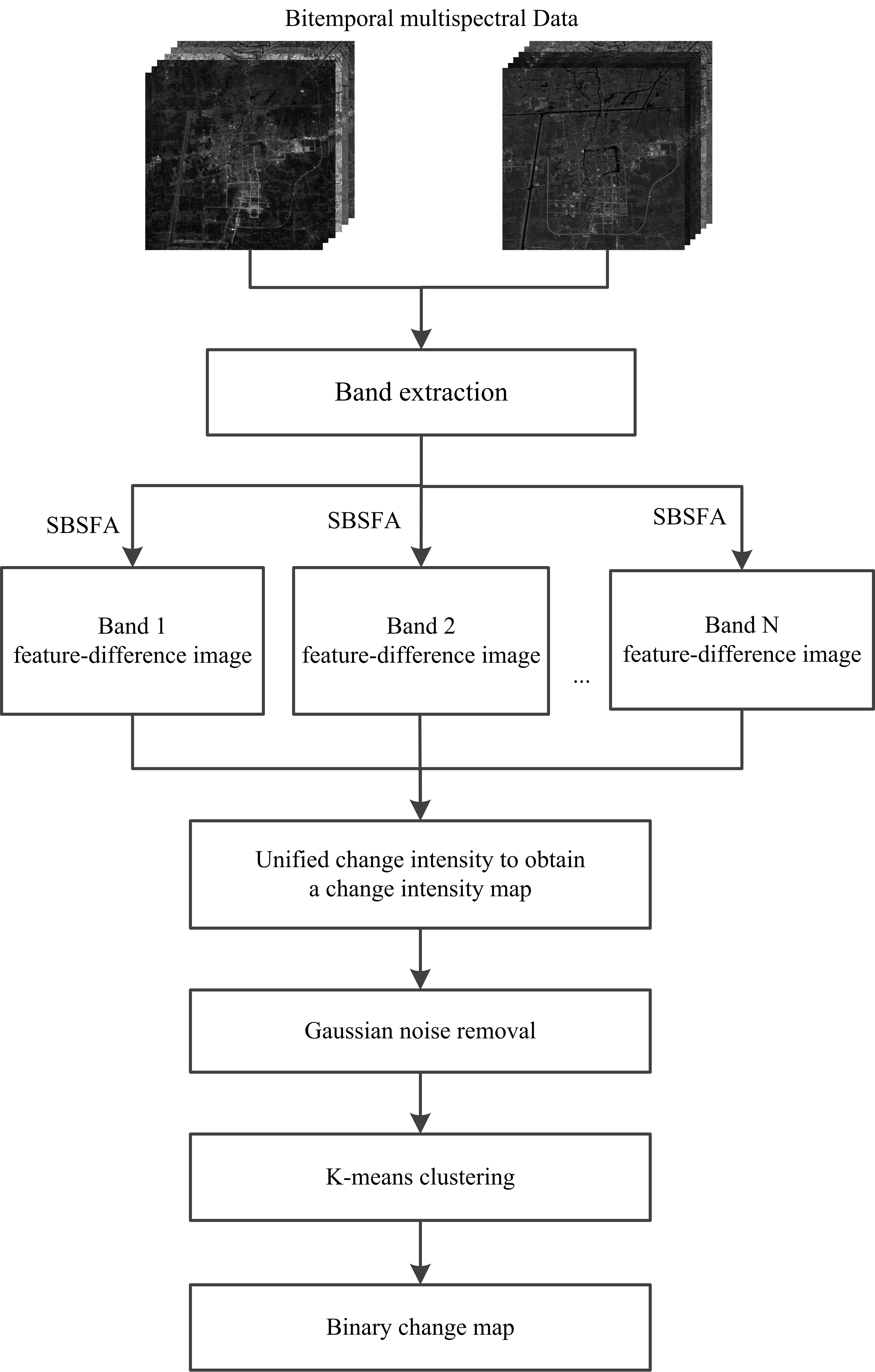
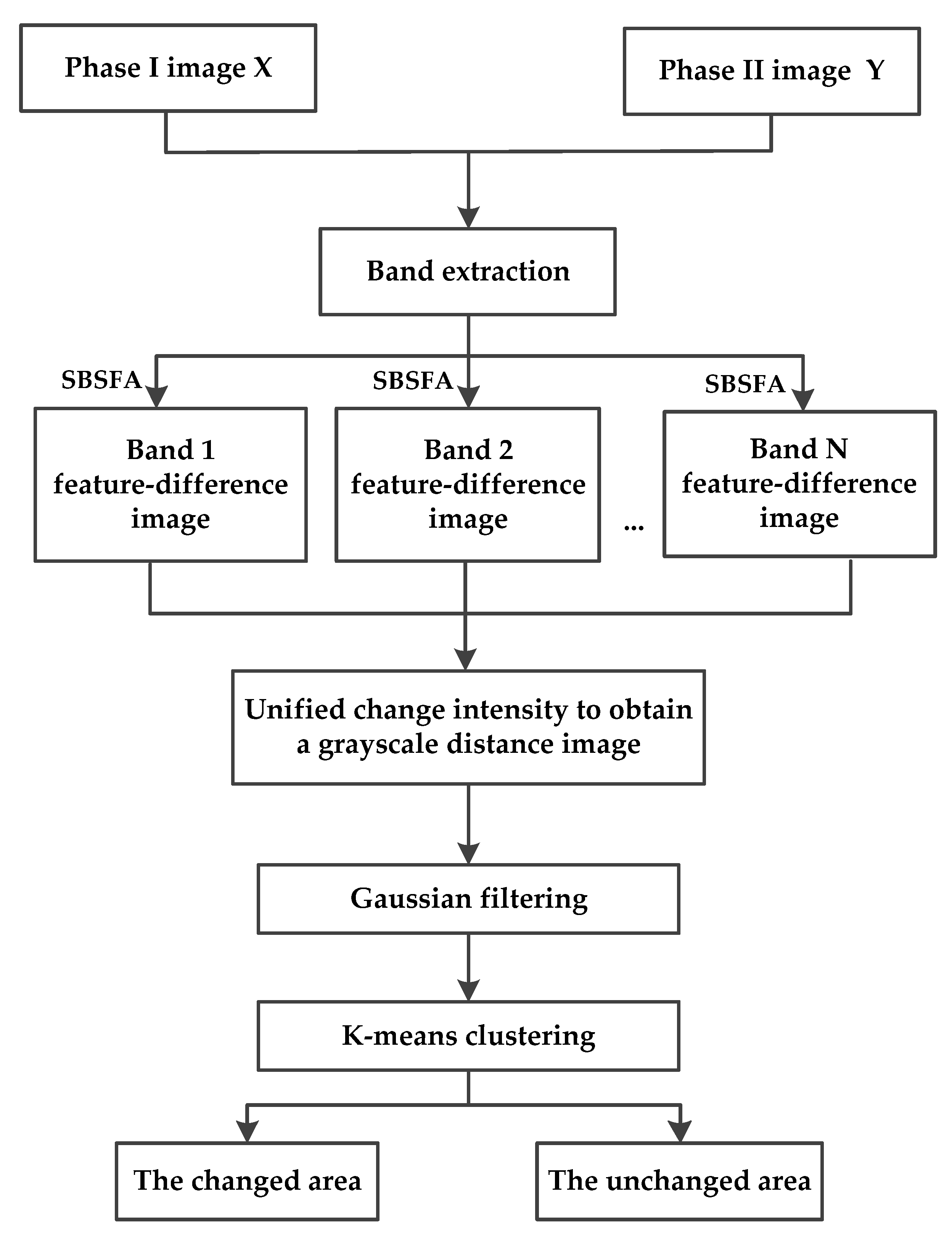
Figure 1 shows a flow diagram of our proposed algorithm. Our algorithm is composed of five steps. First, multiple single-band image pairs are extracted from bitemporal multispectral images. In the second step, single-band slow feature analysis is performed on each pair of single-band images to obtain the optimal feature-difference image of each band. The third step is to fuse the feature-difference images of each band into a grayscale distance image through the Euclidean distance. The fourth step is filtering. Since the noise in multispectral images is mainly Gaussian noise, this paper chooses a Gaussian filter to denoise the grayscale distance image. Finally, binary clustering analysis of the filtered grayscale distance image is carried out using the k-means clustering method.
The contributions of our work are as follows. First, the shortcomings of the SFA algorithm are analyzed, and a new change detection algorithm is proposed. The idea of minimizing the deviation of the unchanged region of each band is used to process bitemporal multispectral images band by band to effectively highlight the change information of each band. Second, the proposed algorithm is simple in calculation and avoids the high time consumption caused by the huge computation of iterative calculation in our previous study [
23]. Last, a novel simulation dataset is presented to discuss the universality of the change detection algorithm. The characteristic of the dataset is that the simulated changes are more similar to the real ground changes on gray values.
The rest of this paper is organized as follows.
Section 2 introduces related work. In
Section 3, SFA theory and our proposed algorithm are introduced.
Section 4 discusses the experimental results. The complexity and universality of our proposed algorithm are discussed in
Section 5. Finally,
Section 6 provides a conclusion.
3. Methodology
3.1. SFA Theory
SFA is an unsupervised algorithm for learning invariant features, which has been applied to human action recognition [
37], text recognition [
38], and fault detection [
39]. Mathematically, SFA theory can be described as an optimization problem; for a given multidimensional input time signal
, it is expected to find a set of functions
to minimize the time difference of output signals
. Due to the fact that SFA was originally proposed for continuous signals, the time difference is usually expressed as the square of the first derivative of output signals.
The optimization objective of SFA is expressed as Equation (1):
The constraints are written as:
The measures the speed of signal changes; is the first derivative of the output signal; is the mean value in time. Equations (2)–(4) are zero-mean constraint, unit variance constraint, and decorrelation constraint, respectively. The zero-mean constraint simplifies the computation and improves the computation speed; the unit variance constraint avoids constant solutions so that each output signal can carry a certain amount of information; the decorrelation constraint ensures that the output signals are not correlated with each other. After sorting, the first output signal is the slowest signal, the second one is the signal with the second-slowest change, and so on.
Assuming that the signal transformation function is linear, then the output signal can be expressed as Equation (5):
And Equations (1)–(4) should be reformulated as Equations (6)–(9):
If Equation (8) is integrated into Equation (6), the optimization objective function can be rewritten as:
Then, the SFA problem can be solved by the generalized eigenvalue problem:
where
is the mathematical expectation of the covariance matrix of the first derivative of the input time signal;
is the mathematical expectation of the covariance matrix of the input signal;
represents the characteristic vector matrix,
is a diagonal matrix of generalized eigenvalues, where
.
However, there is no such time series structure in bitemporal remote sensing images. To solve this problem, Wu et al. [
18] reconstructed the SFA algorithm into the discrete case by using finite difference instead of the first derivative and applied it to change detection.
Given two centralized and standardized vector
and
, where
and
represent the two spectral vectors at the same position in the bitemporal remote sensing images
and
,
is the serial number of the pixel, and
is the number of bands. Then, matrix A and matrix B can be rewritten as Equations (12) and (13) for remote sensing change detection:
where
and
are covariance matrices of remote sensing images
and
, respectively.
represents the covariance matrix of the original difference image, and P is the number of pixels in a single image.
Taking Equations (12) and (13) into Equation (11), the eigenvector matrix W can be obtained, and the feature-difference matrix SFA is expressed as:
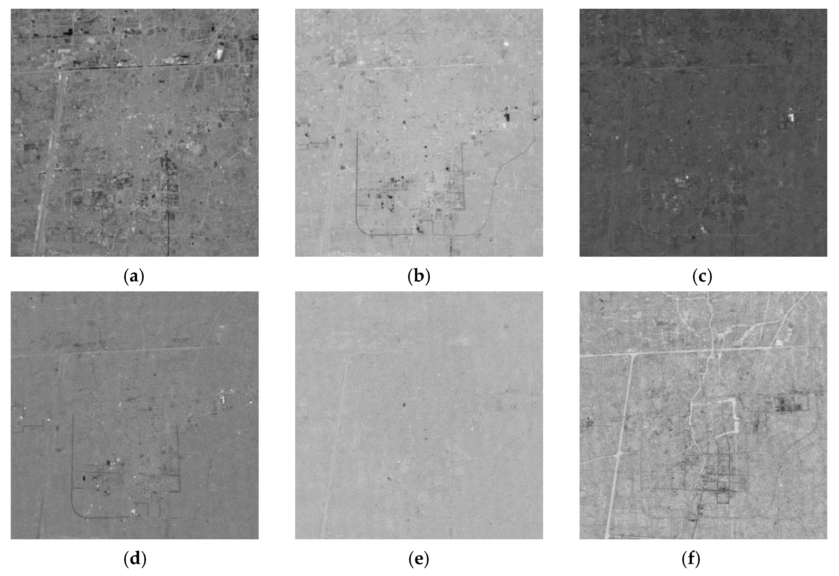
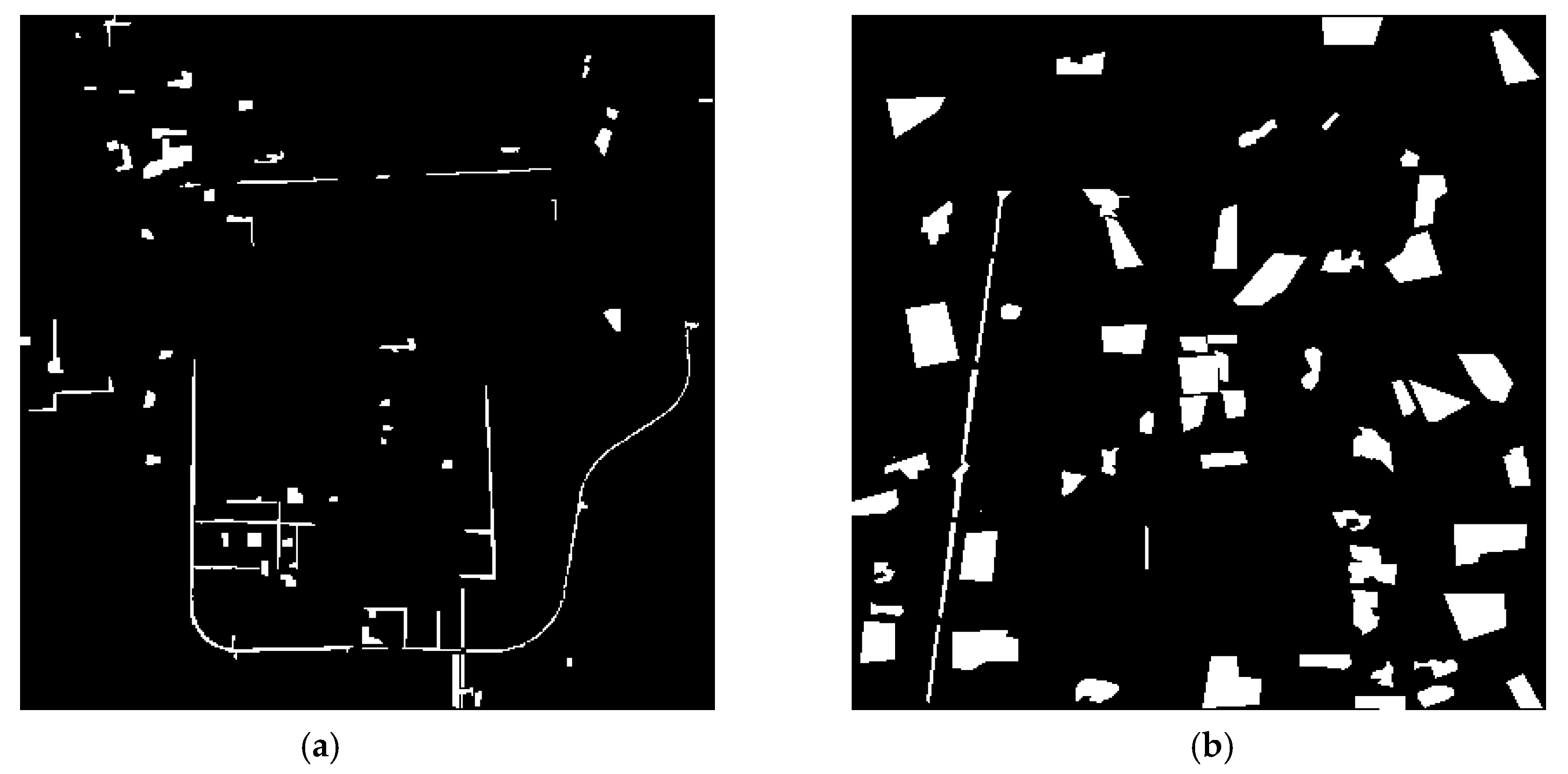
Figure 2 shows six feature-difference images obtained by the SFA algorithm using the Taizhou dataset [
21]. These images are sorted according to the
value from low to high. The lower the ranking, the smaller the feature variance of a feature-difference image. That is, (a) is the feature-difference image with the smallest variance, and (f) is the feature-difference image with the largest variance. In the output results, very dark or bright areas are named marked areas, which represent the areas with a high absolute value of the feature difference. Theoretically, the higher the
value of a feature difference image is, the more change information it contains. It can be seen from
Figure 2a–d that each image contains a certain marked area, but the amount of change information from (a) to (d) does not increase in sequence. Specifically, the marked areas in (b) are closest to the reference change image of the Taizhou dataset, followed by (a) and (d), and finally (c). The changed and unchanged areas of (e) and (f) are not effectively separated. Therefore, visual interpretation shows that SFA theory is difficult to effectively and orderly concentrate the change information to a few feature bands, and the
value cannot be used as a standard to measure the amount of change information.
In order to confirm this subjective opinion, the experiment in
Table 1 is carried out. For each feature band combination in the experiment, Euclidean distance is used to generate a grayscale distance image, and then k-means binary clustering analysis is performed.
Table 1 shows that the combination of feature bands 1, 2, and 4 with clearly marked areas performs best on PCC and kappa, while the combination of feature bands 1–6 has the worst detection results. Based on the subjective evaluation and objective indexes, it can be inferred that a large amount of useless information contained in feature bands 5 and 6 has a negative impact on the detection accuracy, and the change information contained in feature band 4 is more abundant than that in feature band 3. It means that the change information contained in each feature band cannot be measured only by the
value, and the SFA algorithm has the shortcoming of disordered distribution of change information.
3.2. Proposed Method
The purpose of the SFA algorithm is to minimize radiation differences in the unchanged areas to highlight the real changes. However, the shortcoming of the disordered distribution of change information will seriously affect detection accuracy. In order to avoid this problem and further improve the accuracy of change detection, a single-band slow feature analysis method is proposed in this section.
The single-band slow feature analysis algorithm is introduced as follows. First, multiple single-band images are extracted from multispectral images in order of wavelength. Second, the optimal projection vector of a single-band image is found by minimizing the variance of the feature-difference image of the band. Third, the optimal feature-difference images of each band are obtained. In this way, each optimal feature-difference image contains abundant change information. Finally, after the fusion of several feature-difference images, Gaussian filtering is used to obtain the final grayscale distance image. The detailed implementation steps show the following.
First, multiple single-band image pairs are extracted from bitemporal multispectral images. Specifically, multiple single-band images are extracted from multispectral image , and multiple single-band images are extracted from multispectral image . The i-band image pairs are denoted and . By performing zero-centering on each single-band image, the effect of radiation differences can be initially reduced. The processed i-band image pairs are represented as and , where represents the total number of pixels in a single-band image.
Second, the ith projection vector is found by minimizing the variance of the feature-difference image of the i-band, and then, the optimal feature-difference image of the i-band is obtained.
The primary objective of the optimization is expressed as Equation (15):
The constraints are written as:
where
and
are as shown in Equations (18) and (19):
where
is the variance matrix of the i-band difference image, and
and
are the variance matrices of each temporal i-band image.
When Equation (17) is integrated into Equation (15), the objective function can be rewritten as:
With Equations (18) and (19), a new optimization objective can be further obtained:
Since Equation (21) aims to obtain the optimal projection vector
, it can be calculated through Equation (22):
where
,
is the variance of the feature-difference image of the i-band.
The optimal feature-difference image matrix of the i-band is expressed as:
Third, the
grayscale distance matrix is calculated. Repeating the previous steps, the optimal feature-difference image matrix of each band is obtained. After adjusting the difference matrix
into a column vector, the difference matrix
is expressed as:
Then, the difference matrix is converted into the grayscale distance image matrix by Equation (25) (the Euclidean distance formula), and the changed intensity of pixels in each band is unified.
Finally, the grayscale distance image is processed by a Gaussian filter to further eliminate false changes.
In order to measure the impact of the Gaussian filter on the performance of the proposed algorithm, the experiments in
Table 2 are carried out by using the Taizhou dataset. In this experiment, the standard deviation of Gaussian filters is set to 1. The results show that Gaussian filtering can effectively reduce FN and FP, and improve the accuracy of change detection. The precision of the 7 × 7 filter window is the highest. For the sake of simplicity, the Gaussian filter with a 7 × 7 window is used in the following experiments.
4. Experiments
To verify the advantages of our proposed algorithm, some popular pixel-level methods, such as CVA [
8], PCA [
10], MAD [
12], IR-MAD [
31], SBIW [
23], SFA [
18], ISFA [
19], and DSFA [
21], were selected for comparison. Specifically, the convergence thresholds of IRMAD, SBIW, and ISFA were all set to 10
−6; the DSFA algorithm selected in experiments has two hidden layers, each with 128 nodes. To ensure the comparability of results, the Gaussian filter was used for the grayscale distance image generated by each algorithm, and the k-means clustering algorithm was used in all the above methods to obtain the binary change map. It should be noted that the DSFA algorithm was implemented by Python, and other algorithms were implemented by MATLAB. The following experiments were performed on an Intel Corei5 1.6 GHz CPU equipped with 8 GB RAM.
Experiments were carried out on three bitemporal remote sensing image datasets. These datasets include two common multispectral change detection datasets and one simulation dataset. The first dataset is the Taizhou dataset [
40]. Two multispectral images were obtained on 17 March 2000, and 6 February 2003, respectively. The second dataset was before and after the fire in Bastrop County, Texas in 2011 [
41]. The two datasets were obtained by Landsat7 and Landsat 5 satellites, respectively. Six bands (bands 1–5 and 7) with a spatial resolution of 30 m were selected for the experiment. The third dataset was a self-made simulation dataset, detailed in
Section 4.3.
The advantages and disadvantages of these algorithms were analyzed from two aspects of objective and subjective. The objective indexes included false negative (FN), false positive (FP), overall error (OE), percentage correct classification (PCC), kappa coefficient (KC), and time complexity. FN is the number of samples that are erroneously labeled as unchanged. FP represents the number of samples that are erroneously labeled as changed. OE indicates the sum of FN and FP; the closer OE, FP, and FN are to 0, the better the change detection performance. PCC is the proportion of correctly labeled samples in all samples. Kappa coefficient is a parameter that can accurately measure the classification accuracy; the closer its value is to 1, the more accurate the classification. Time complexity is a very important indicator, which measures the computational efficiency of an algorithm. To further reduce experimental errors, the time complexity in this paper refers to the average running time of an algorithm. The average running time is the average of 10 runs.
4.1. Experimental Dataset I
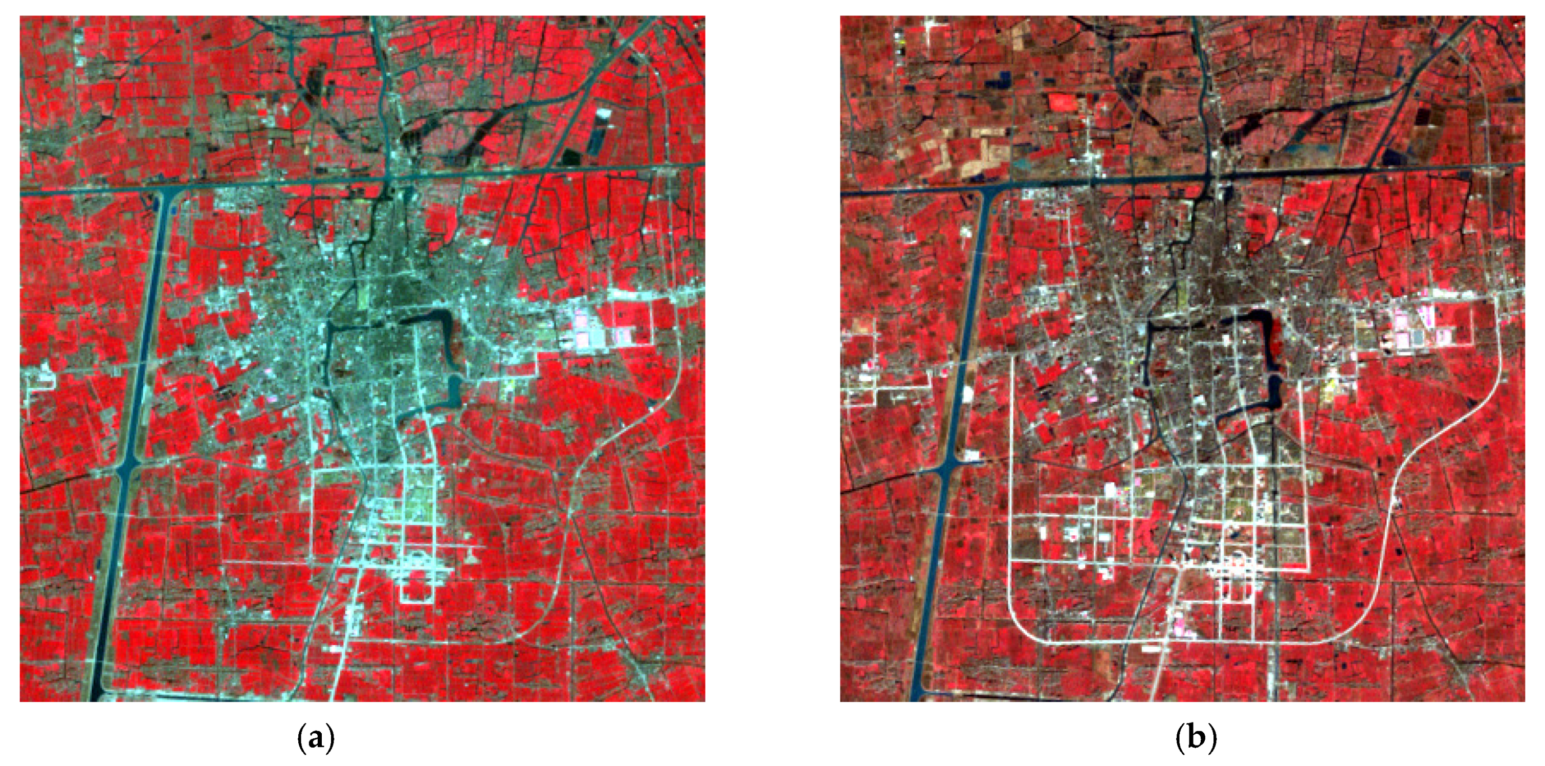
The first dataset comprises bitemporal multispectral remote sensing data from Taizhou City, Jiangsu Province. Two multispectral images were obtained on 17 March 2000, and 6 February 2003, respectively. The two images in
Figure 3 are pseudo-color composite images of multispectral data of Taizhou, and each image contains 400 × 400 pixels. To objectively evaluate the proposed change detection algorithm, 21,390 test samples (13.4% of the image) provided by the dataset were used for quantitative analysis. The test samples include 4227 changed samples and 17,163 unchanged samples, as shown in
Figure 4.
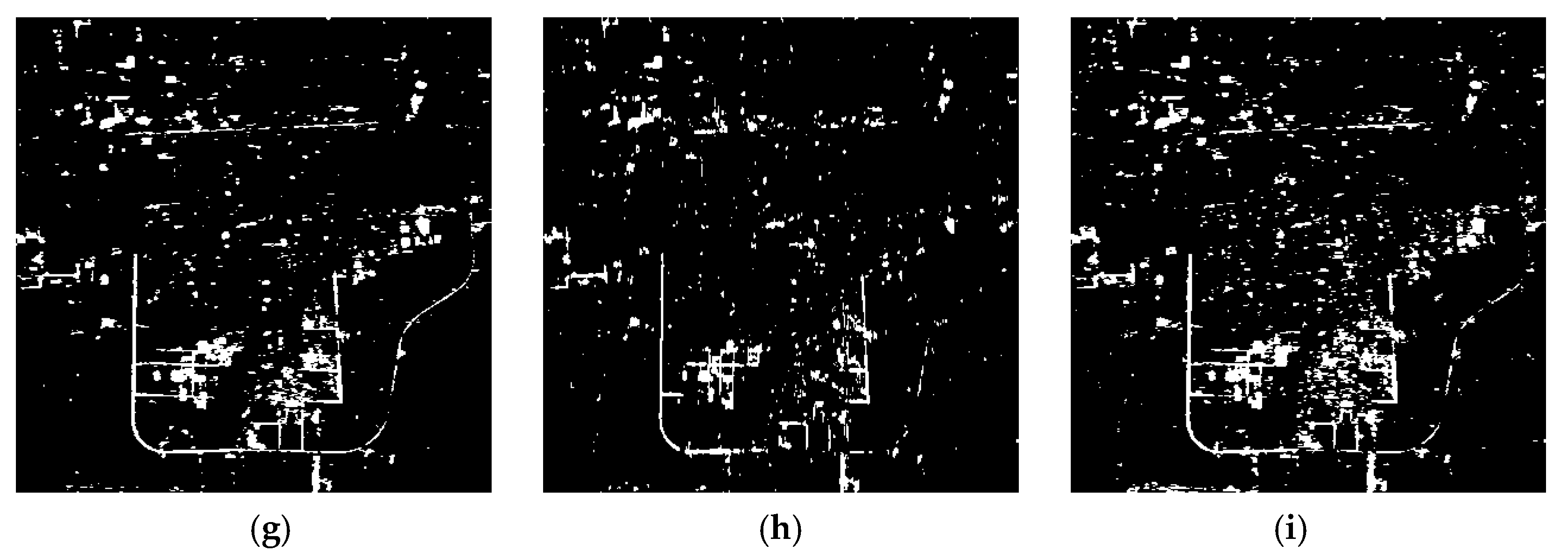
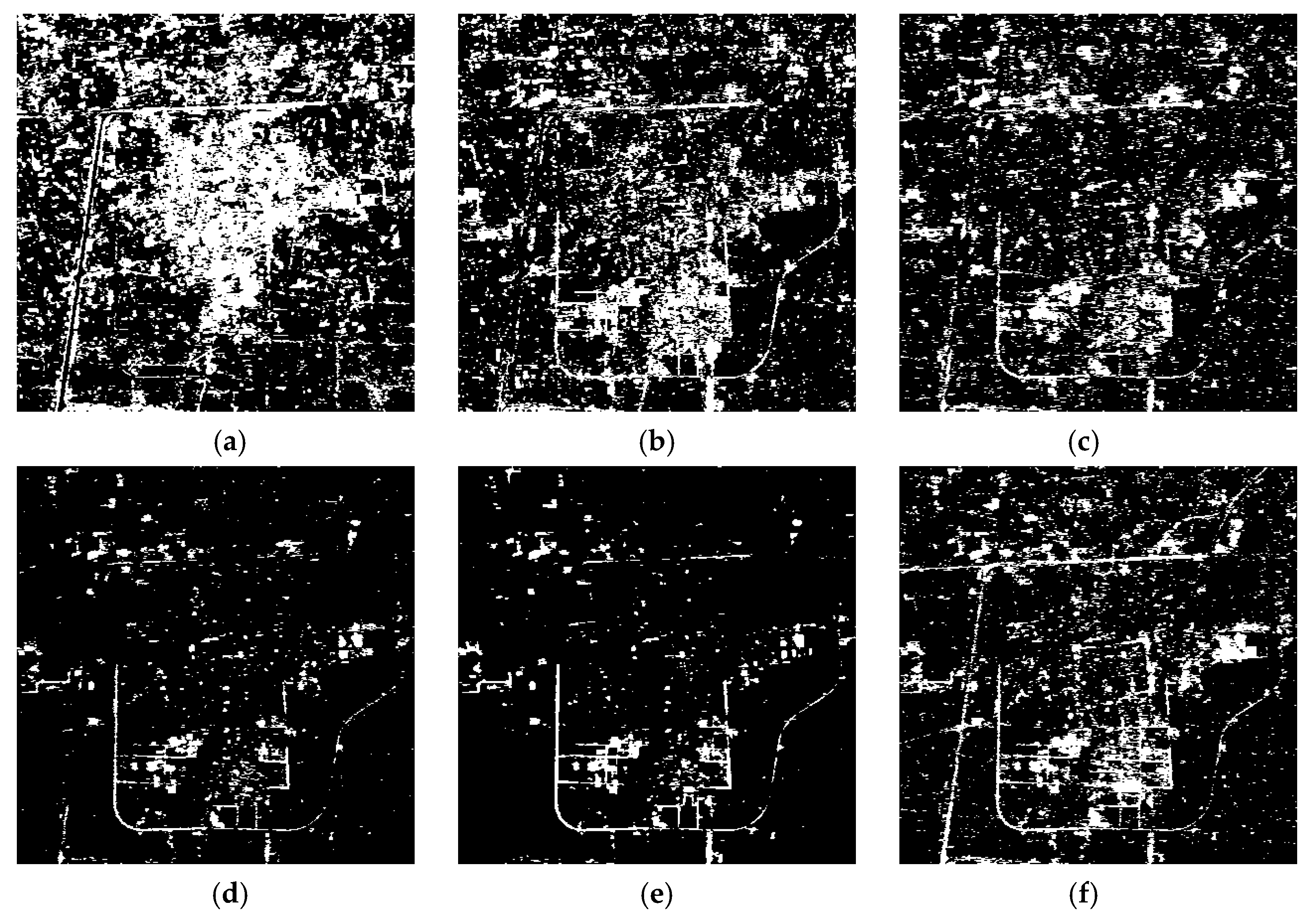
Binary change images obtained by eight comparison methods and the proposed method are shown in
Figure 5. It is obvious that panels (a), (b), (c) and (f) have a large number of broken and small change areas, which indicates that the performances of CVA, DPCA, MAD, and SFA are not ideal for multispectral image change detection. Referring to the reference change sample, panel (h) seems to lose part of the change information. For panels (d), (e), (g) and (i), though there are some change points in the unsampled area, these points may represent the real changed pixels of the unsampled area. Therefore, it is impossible to visually judge which method has better performance.
In order to fairly evaluate the comparison methods and our proposed method,
Table 3 and
Table 4 show the objective evaluations of each algorithm with and without the Gaussian filter, respectively. According to
Table 3 and
Table 4, the detection performance of CVA is the worst, and the performances of MAD and SFA are also not ideal. The PCC and kappa performance of IR-MAD, ISFA, and SBIW are effectively improved through iterative weighting, but the time cost of these algorithms increases significantly. Without using a Gaussian filter, the OE of our proposed algorithm is the lowest, and the kappa coefficient of our proposed algorithm is higher than SFA, ISFA, and DSFA.
Table 3 shows that the kappa of our proposed algorithm is 24.04% higher than that of SFA, 0.15% higher than that of ISFA, and 11.62% higher than that of DSFA. After Gaussian filtering for the grayscale distance image, the accuracy of most algorithms was improved to a certain extent, which proves that this filtering strategy can effectively improve the performance of change detection. Although the kappa of our algorithm was slightly lower than that of ISFA after adding the filter, our algorithm has more advantages in time cost. In summary, our proposed algorithm has obvious advantages in both kappa value and time cost, which indicates that our proposed algorithm is an effectively improved algorithm.
4.2. Experimental Dataset II
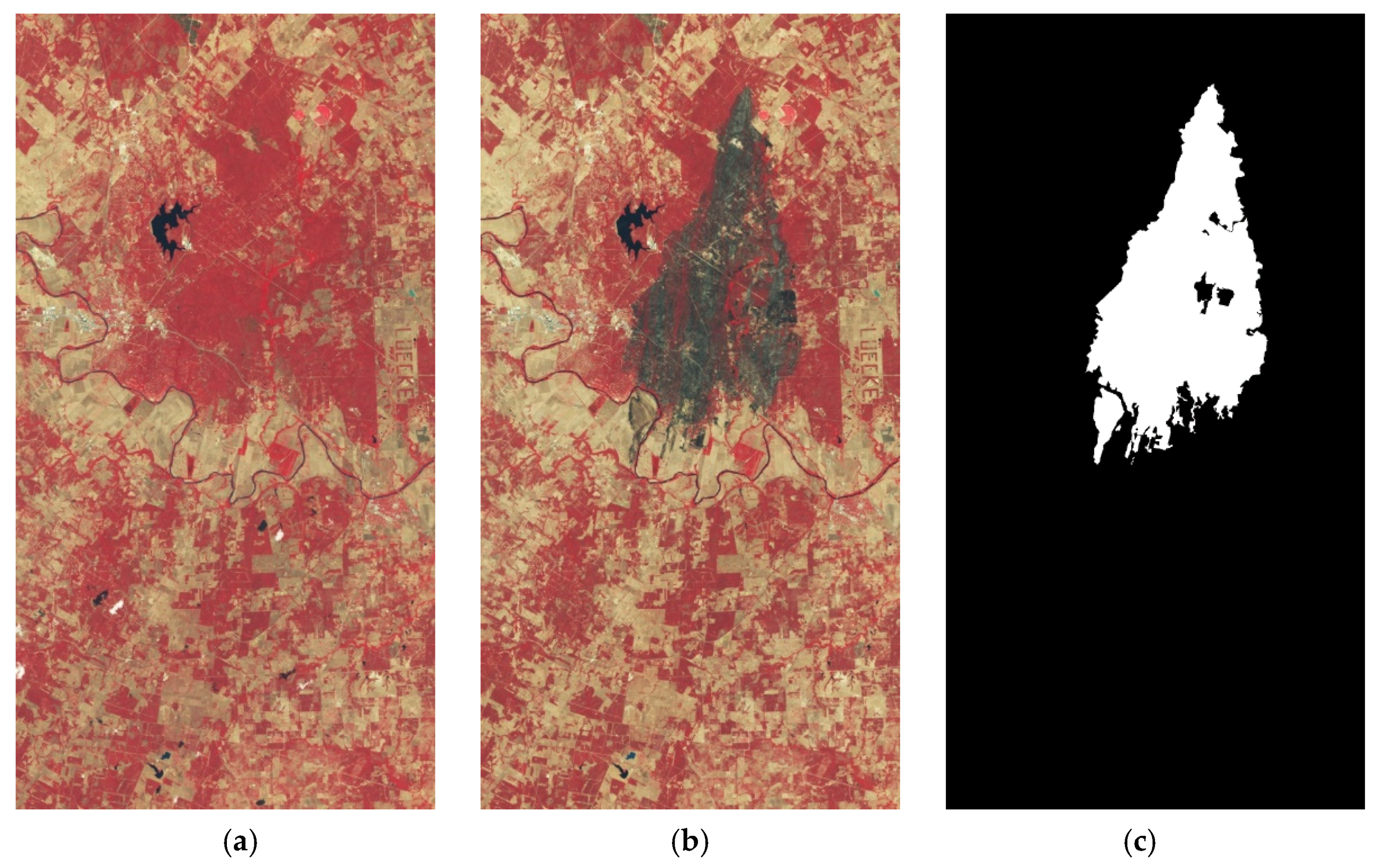
The second dataset is the Texas fire dataset.
Figure 6a is the pseudo-color composite before the Texas fire, and
Figure 6b is the pseudo-color composite after the fire. The image size is 1534
808. In panels (a) and (b), the red parts indicate the safe areas, and the black parts indicate the burning or burned areas. The difference between these pre-event and post-event pairs is only due to the burning of the forest. The reference map (c) is marked as changed and unchanged at the pixel level, in which the white parts (10.64% of the image) represent the changed areas caused by wildfire.
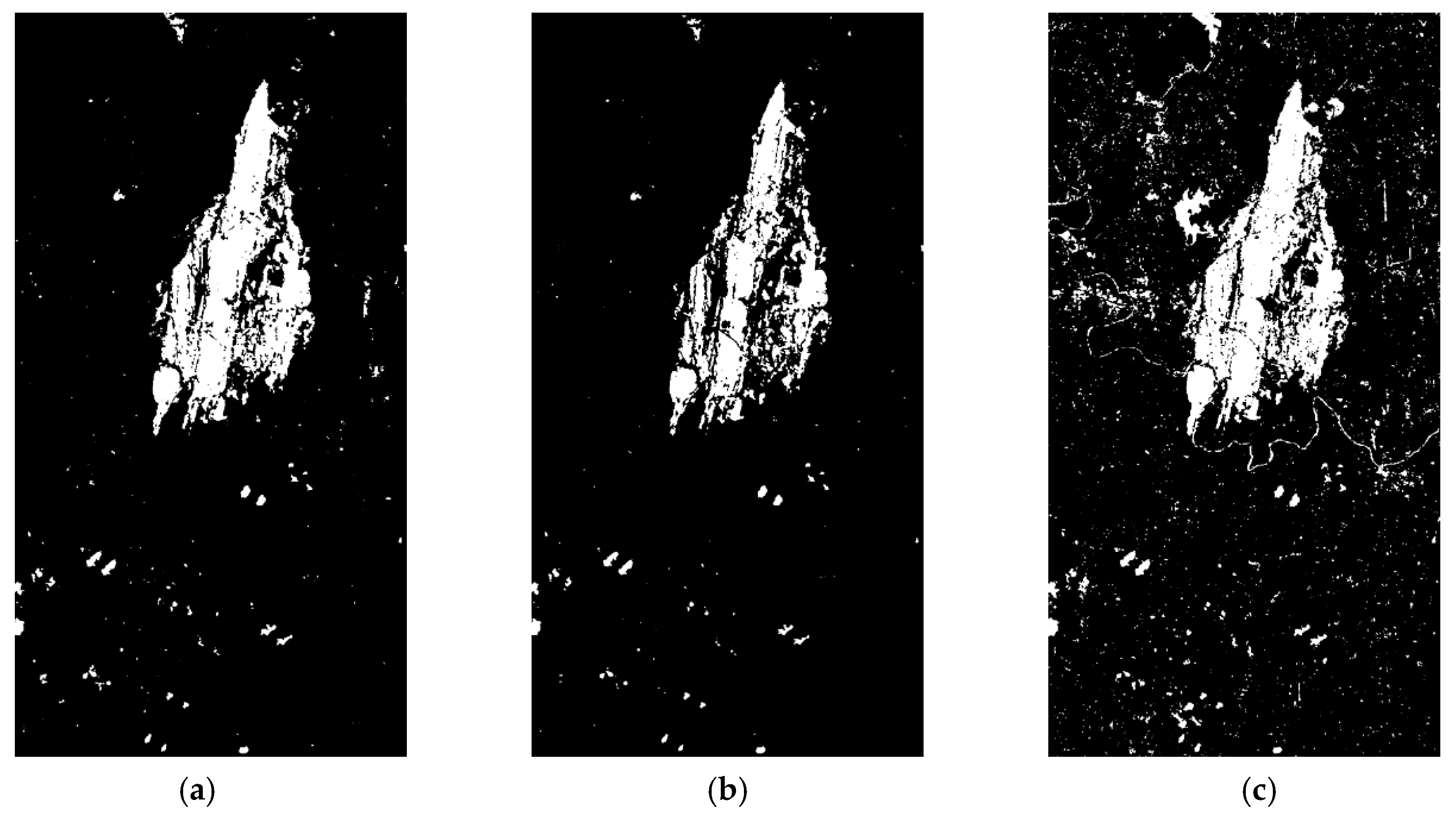
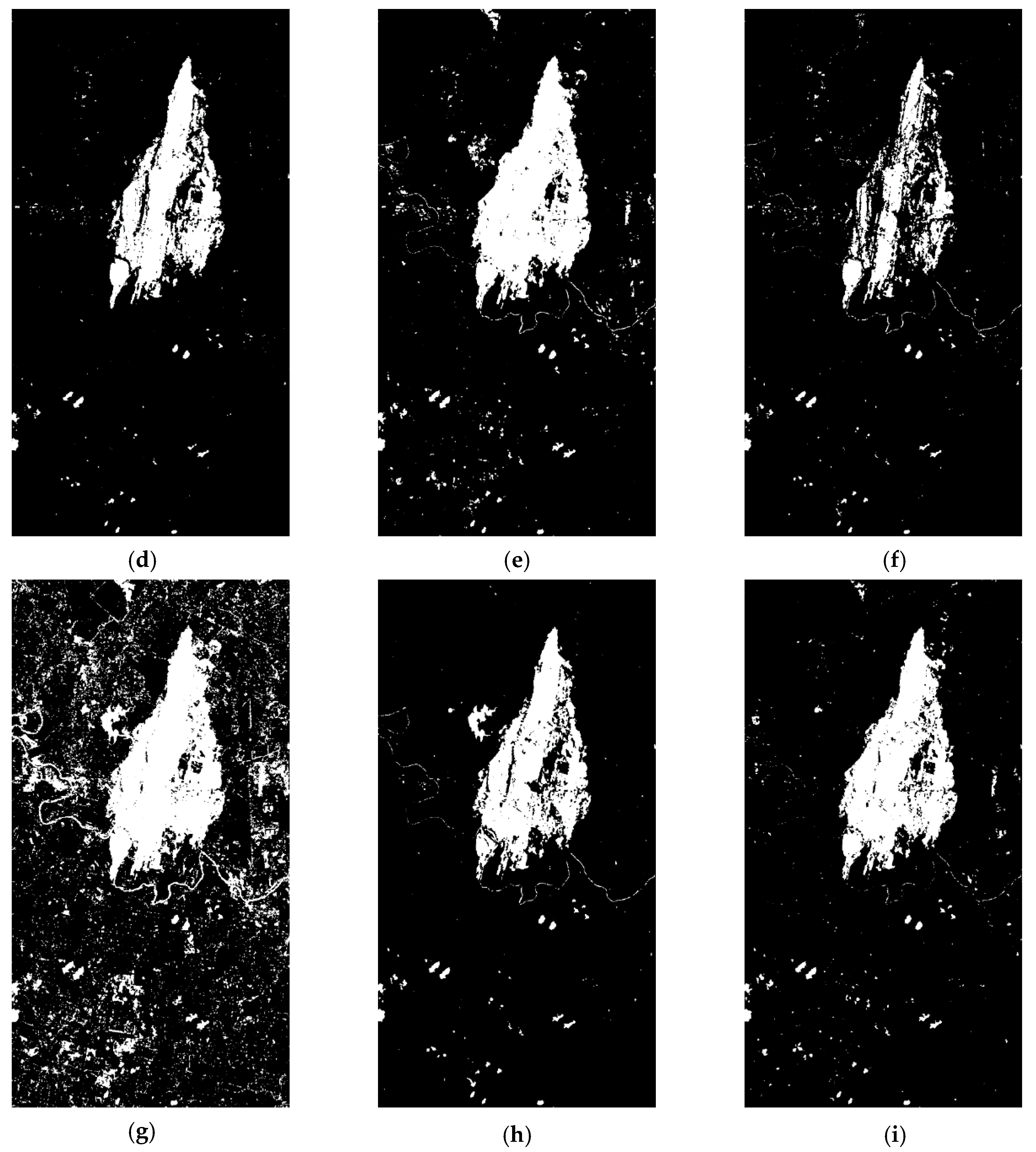
As can be seen from
Table 5 and
Figure 7, MAD and ISFA have a large number of false change points, which means that their inhibition effect on the radiation difference of background area is not ideal. The FN of DPCA and SFA are much higher than other algorithms, which means that these two algorithms have poor performance in detecting changes. Although the performance of our proposed algorithm on FN and FP is not the best, its overall performance is relatively balanced. Its OE is the lowest among all algorithms, and the PCC and kappa are the highest among all algorithms, which are 0.9750 and 0.8690, respectively. Compared with SBIW, our proposed algorithm has a great advantage in time consumption. Considering the precision and time complexity, our algorithm has excellent change detection performance.
4.3. Experimental Dataset III
In this section, we adopt an artificial simulation dataset as dataset III. Compared with a real multispectral image dataset, an artificial simulation dataset provides a simpler and easier way to obtain the reference change map to analyze the experimental results objectively. In the artificial simulation dataset, the first image and the second image are usually multispectral images taken on different days in the same year and month. The artificial change areas are added to the second image to simulate real changes. The specific procedures are as follows: First, the vegetation pixel block with a certain size is obtained from the first band image and spliced into a specific shape of region M1; second, a region, N1, in the first band image of the second phase is replaced by region M1 to simulate a changing region (the shape and size of the region M1 and N1 are the same, but they contain different ground feature information); finally, the above steps are repeated for the remaining bands. Specifically, a vegetation pixel block is intercepted from the i-band image and spliced into the region Mi. The position of the captured pixel block corresponds to the previous operation, and the size of Mi is consistent with that of M1. Then, the region Ni in the i-band image of the second phase is replaced by the region Mi, and the position of the replaced area is the same as for the first band image. In this way, the simulated changes are more consistent with the real ground changes on the gray value. In addition, this simulation method can conveniently obtain an accurate reference map to objectively analyze the detection results and test the effectiveness of the algorithm.
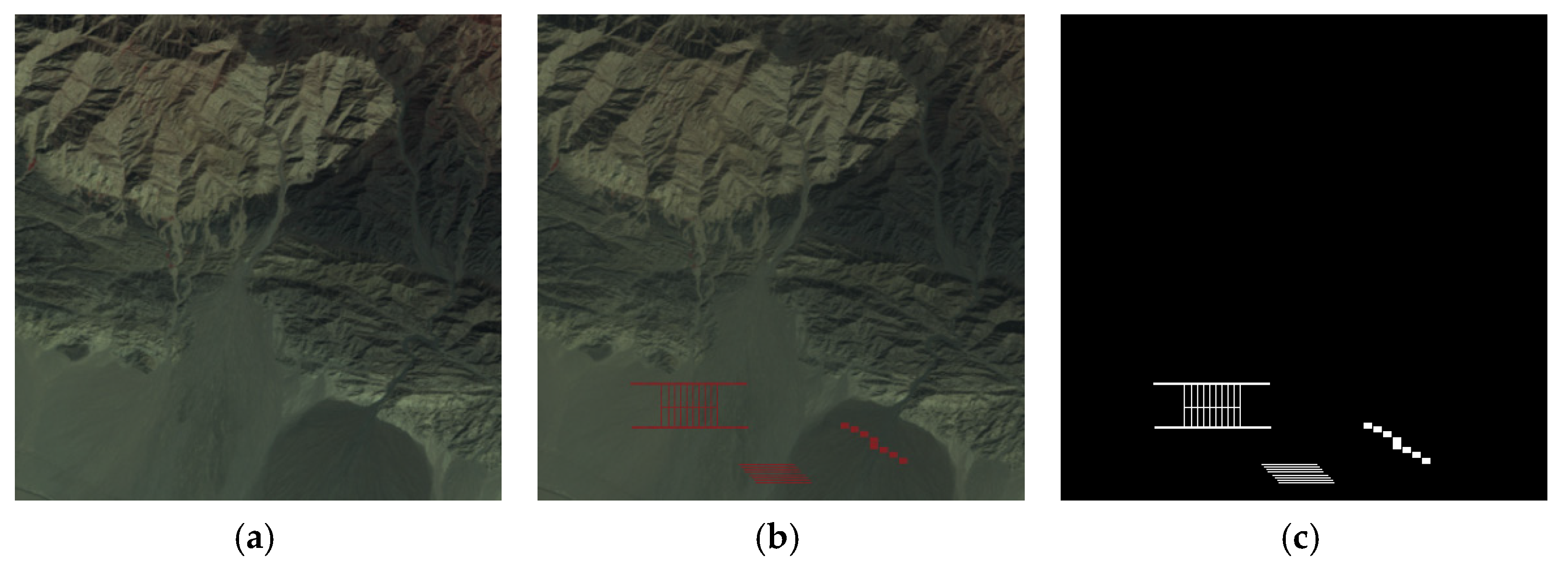
Dataset III includes two multispectral images taken from Bayingoleng, Xinjiang, China. The first multispectral image and the second multispectral image were taken by Landsat 5 on 13 September and 29 September 2007, respectively. Both images have seven bands, and six visible bands (bands 1–5 and band 7) were selected for the experiment. In the latter image, the artificial change region was added to obtain the second-stage multispectral image to be detected.
Figure 8a shows a pseudo-color display of the first multispectral image.
Figure 8b shows a pseudo-color display of the second-stage multispectral image, and the red area in this figure is the simulated change area. The binary reference map is shown in
Figure 8c.
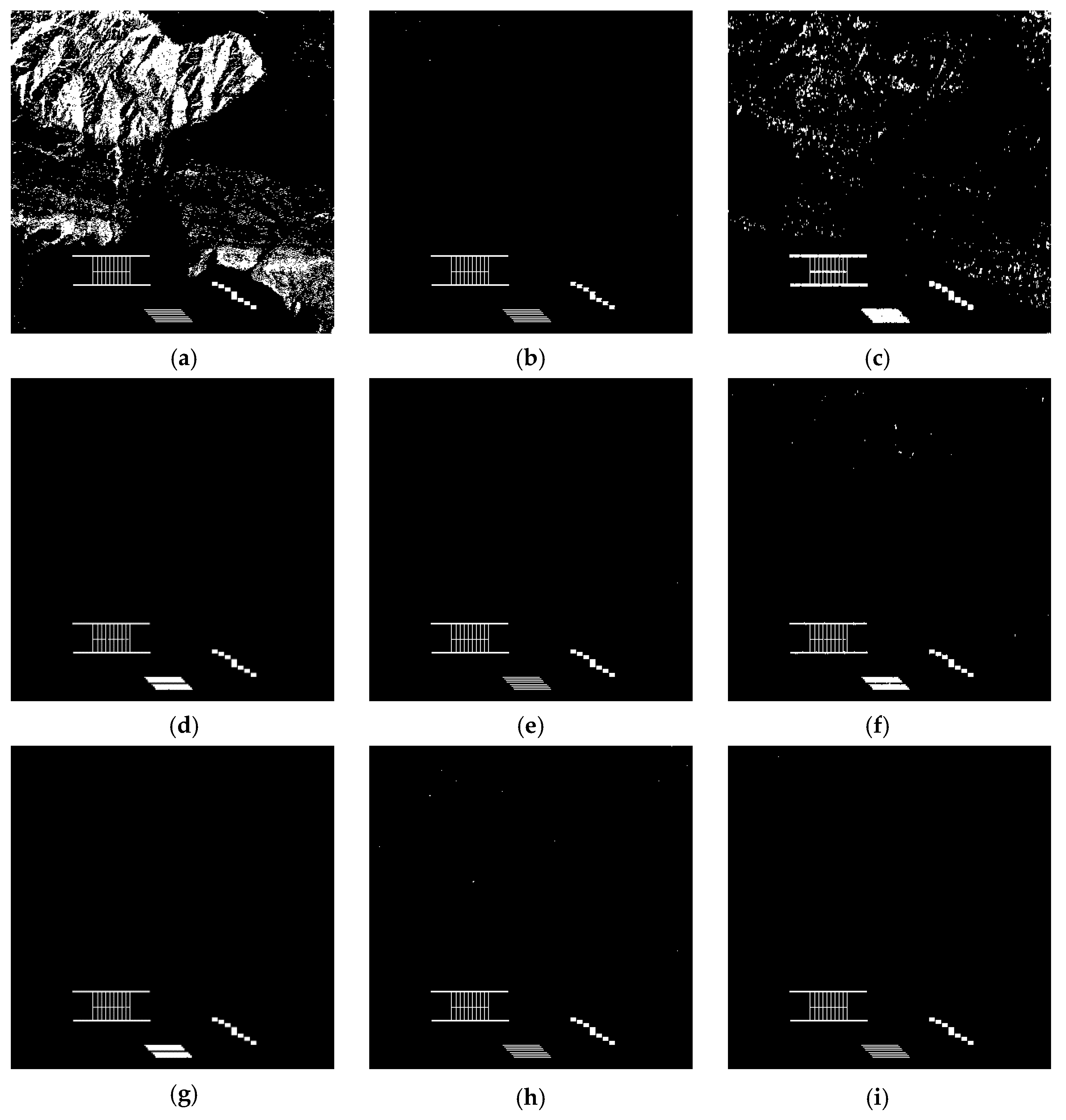
As shown in
Figure 9 and
Table 6, for CVA, MAD, and SFA, the FPs of these three algorithms are obviously high. Although IRMAD, ISFA, and DSFA have fewer FPs, these improvements are achieved at the cost of time. The experimental results of DPCA show that it has good performance in time complexity, but the overall error needs to be further reduced. The SBIW algorithm and our proposed algorithm have the highest detection precision and kappa coefficient. This is because these two methods fully utilize multiband information to detect the changed area in more detail. However, in terms of time complexity, our proposed algorithm outperforms the SBIW algorithm. Considering the time complexity and accuracy, our proposed algorithm is better than other reference algorithms.
5. Discussion
From all the aforementioned experiments, we can see that our proposed algorithm can well suppress the background and noise information in multispectral images, and achieve good performance in change detection accuracy. However, the results also show that our algorithm is not good enough to keep the edge information with weak change intensity. As shown in
Figure 5i, the road detected by our method is discontinuous. In addition, our proposed method only uses the spectral feature for change detection, so that false change points may appear in the water area (as shown in
Figure 7i).
To further verify the universality of our algorithm, 50 groups of artificially generated simulation datasets are created by using the method proposed in
Section 4.3. Compared with marking the changed area based on personal experience, it is convenient to make the change reference map for objective analysis by manually adding some change areas. Therefore, using simulation data set for change detection can effectively evaluate the advantages and disadvantages of our algorithm and reference algorithm. Due to the limitation of the paper, the average change detection results can be found in
Table 7.
Table 7 shows that the total number of error pixels of the proposed algorithm is 52, which is the second lowest among all algorithms, and compared with other algorithms, it has apparent advantages over the PCC values and kappa coefficient. Specifically, the PCC of our proposed algorithm is 2.77% higher than that of SFA, and the kappa coefficient is 25.42%, 7.97%, and 9.45% higher than that of SFA, ISFA, and DSFA, respectively. Compared with SBIW, the proposed algorithm avoids the high time consumption caused by the large amount of iterative computation in previous work. While maintaining the same excellent detection accuracy, the detection time is greatly shortened. The advantages and universality of the proposed algorithm are fully verified by these experiments with 50 datasets.


