Abstract
Object detection based on remote sensing imagery has become increasingly popular over the past few years. Unlike natural images taken by humans or surveillance cameras, the scale of remote sensing images is large, which requires the training and inference procedure to be on a cutting image. However, objects appearing in remote sensing imagery are often sparsely distributed and the labels for each class are imbalanced. This results in unstable training and inference. In this paper, we analyze the training characteristics of the remote sensing images and propose the fusion of the aggregated-mosaic training method, with the assigned-stitch augmentation and auto-target-duplication. In particular, based on the ground truth and mosaic image size, the assigned-stitch augmentation enhances each training sample with an appropriate account of objects, facilitating the smooth training procedure. Hard to detect objects, or those in classes with rare samples, are randomly selected and duplicated by the auto-target-duplication, which solves the sample imbalance or classes with insufficient results. Thus, the training process is able to focus on weak classes. We employ VEDAI and NWPU VHR-10, remote sensing datasets with sparse objects, to verify the proposed method. The YOLOv5 adopts the Mosaic as the augmentation method and is one of state-of-the-art detectors, so we choose Mosaic (YOLOv5) as the baseline. Results demonstrate that our method outperforms Mosaic (YOLOv5) by 2.72% and 5.44% on 512 × 512 and 1024 × 1024 resolution imagery, respectively. Moreover, the proposed method outperforms Mosaic (YOLOv5) by 5.48% under the NWPU VHR-10 dataset.
1. Introduction
Object detection is a key component of remote sensing research [1,2,3] and plays a crucial role in the fields of urban planning, environment monitoring, and borderland patrol [4,5,6]. Studies on object detection-based methods have made great progresses in recent years [7,8], particularly for deep learning applications [9,10]. To further improve the training performance and efficiency, numerous training strategies have been proposed, including loss function design, data augmentation, and regularization techniques. In order to prevent overfitting or the excessive focus on a small set of input training objects, random feature removal (e.g., dropout) has been developed. The dropout randomly deletes neural nodes or erases some regions. While the regional dropout method has improved the generalization of object detection tasks, the training of convolutional neural networks is a data-driven process, and current object detection methods are limited by a lack of training data. In the field of object detection, basic augmentation methods are typically combined with cropping, rotation, translation, and color jittering, and semantic augmentation methods are composed of background and shape changes (Figure 1). The basic augmentation only augments the objects and neglect the significance of multiple backgrounds.
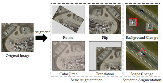
Figure 1.
Basic training data augmentation methods.
In order to efficiently use the training samples, multiple images can be adopted into a single training image via approaches that mix training samples (e.g., CutMix [11], MixUp [12], and Mosaic [13]). However, objects in remote sensing images are typically sparsely distributed, and those sample fusion methods will result in blank training samples (Figure 2). Moreover, the class labels in the remote sensing images are often imbalanced, and thus these objects appear in few images or scenes. The synthetic sample and re-sampling methods proposed to overcome these problems are pre-processing procedures, and are not able to balance the training samples automatically and dynamically.
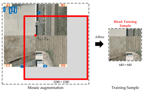
Figure 2.
Mosaic augmentation generates training samples by randomly selecting four images and splicing them together.
The aim of the current paper is to design mosaic training methods for remote sensing images with a sparse object distribution. We address this by introducing the Aggregated-Mosaic Training augmentation strategy. Based on the state-of-the-art detector Yolov5 [13] and the augmentation method Mosaic, our contributions are summarized as follows:
- (1)
- We analyze the object distribution of remote sensing images and highlight the problem of augmentation in object samples with a sparse distribution. We introduce Assigned-Stitch, a constraint for sparse object augmentation, which guarantees that each training sample is not a blank sample and ensures a smooth and stable training procedure;
- (2)
- We propose the Auto-Target-Duplication modules to overcome the class-imbalance problem. This module is able to balance the labels of each class and focus on the poor class results by efficiently selecting objects to duplicate.
The rest of the paper is organized as follows. In Section 2, related work, such as object detection and data augmentation, is reviewed, while the proposed Aggregated-Mosaic Training method is detailed in Section 3. In Section 4, we present two datasets and describe the experimental results. Section 5 concludes the paper and outlines future research directions.
2. Related Work
2.1. Object Detection
Over the last decades, the object detection has developed quickly, and this development composes of two stages. First, the hand-crafted features [7,14] and discriminative classifiers [15,16] are combined for object detection, such as in a Deformable Part Model (DPM) [8,17]. Second, as the hand-crafted features can make it hard to distinguish between objects and backgrounds, the convolution features come to the fore, along with the quick development of the computing power. The convolution neural-network-based classification method was first proposed in 2012 at the ImageNet Large Scale Visual Recognition Challenge (ILSVRC 2012) [18]. More specifically, Krizhevsky et al. proposed AlexNet [19], based on convolutional layers, fully connected (FC) layers, and a simple softmax classifier, which transfers the convolutional neural networks (CNNs) into the computer vision tasks. There are currently two object detection framework classes.
One-stage object detection: Joseph et al. proposed You Only Look at Once (YOLO) [20], which performs the detection procedure as a regression task. Liu Wei et al. subsequently proposed a Single Shot multibox Detector (SSD) [21], which combines the anchor strategy in Region with Convolutional Neural Networks (R-CNN) [22] and the regression in YOLO to increase accuracy and detection speed. Following this, Yolov2 [23] was proposed, which includes multi-scale training and hierarchical classification, resulting in both a fast detection speed and high accuracy. Yolov3 [24,25] adopts Feature Pyramid Network (FPN) [26], darknet-53, and binary cross entropy loss to balance the model size and detection speed, resulting in a 100x greater detection speed compared with fast R-CNN [27]. Yolov4 [28,29] combines multiple optimization methods (e.g., mosaic data augmentation, self-adversarial-training, mish-activation, and CIoU [30,31] loss) to attain a higher detection accuracy. Based on its predecessors, the state-of-the-art detector Yolov5 [13] adopts a hyper-parameter to balance the model size and detection speed. In the current paper, we adopt Yolov5 as the baseline.
Two-stage object detection: Ross et al. proposed the first CNN-based object detection framework, denoted as R-CNN [22]. CNN features have been proven to demonstrate a greater discrimination between objects and backgrounds compared to hand-craft features. Fast R-CNN [27] and Faster R-CNN [32] were subsequently proposed, accelerating the detection within a region. Mask R-CNN [10] employs multi-task training for object detection and instance segmentation. By accounting for the large amount of computation in the localization procedure, the CenterNet [33] regards the object as a center point and regresses the bounding box. Following Mask R-CNN, D2Det [9] adopts dense local regression and discriminative RoI pooling to enhance the detection and instance segmentation performance.
2.2. Data Augmentation
Random dropout: The dropout concept can be divided into two categories: (i) In the neural network dropout, dropout series methods [34,35] randomly mask a set or region of neural units for robust hyper-parameters. (ii) The training image dropout approach employs Random Erase (RE) [36] to solve overfitting during training and object conclusion by randomly selecting a rectangle region in the training samples and erasing pixels with random values. Following RE, CutOut [37,38] randomly masks out square regions of input training samples, improving the robustness and performance of classification CNNs. The Assigned-Stitch module proposed in this paper adopts random cut and translation, which also involves the random dropout concept.
Training data generation: In order to overcome the lack of training samples and to improve the neural network generalization, much research has explored data generation techniques. Cut Paste Learn (CPL) [39] cuts object instances and pastes them on random backgrounds, which relieves expensive data collection costs. Then, Dvornik et al. [40] improves on this and leverage segmentation annotations by increasing the number of object instances presented in the training data. Geirhos et al. uses stylized-imagenet [41], a stylized version of imagenet, to learn a texture-based representation for shape-based feature representation. The proposed Aggregated-Mosaic is able to generate numerous remote sensing training samples. In particular, it ensures that each training sample contains multiple objects with sparse distribution scenes and, based on the evaluation results, Auto-Target-Duplication automatically pastes classes associated with poor results.
Multiple sample fusion: Multiple sample fusion is currently the focus of much attention due to its effective use of the training dataset. Mixup [12] trains a convolutional neural network on convex combinations of image pairs and labels. Between-Class (BC) [42] mixes two images belonging to different classes with a random ratio. This technique can also work on sounds. Several descendant mixing methods have been proposed based on these fusion techniques. Random Image Cropping and Patching (RICAP) [43] randomly crops four images and patches the images and labels to create a new training sample. Then, CutMix [11] cuts and pastes patches among training sets, and the ground truth labels are also mixed proportionally to the area of the patches. Note that CutMix mixes just two input images, while Yolov4 proposes the Mosaic method [28], which mixes four training images and allows the detection of objects outside their normal context. These multiple sample fusion methods are powerful when applied to natural images. However, the objects in remote sensing images are often distributed sparsely, and thus these multiple sample fusion methods typically generate training samples with no objects, leading to unstable training and inference procedures. With a focus on remote sensing imagery with sparse objects, the proposed Aggregated-Mosaic employs training sample fusion, and also solves the problem of blank training sample.
Generalization tricks: Due to the requirement of a large amount of training data, ensuring the efficient training of a convolutional neural network is crucial in object detection and classification. Batch Normalization (BN) [44], Adam [45], and weight decay [46] are widely employed in training procedures. In order to combat adversarial training samples [47], several approaches include the addition of noise to feature maps, and manually set a network shortcut to enhance the performance [48]. Then, Multi-Objective Genetic Algorithm (MOGA) [49], Selective Sparse Sampling Networks (S3Ns) [50], and virtual image generation [51] are proposed for the sparse object representation. Distinct from the aforementioned generalization tricks, the proposed Aggregated-Mosaic enhances the performance on the data level, without altering the architecture and feature representations. This allows its application in methods involving remote sensing images with a sparse object distribution.
3. Methods
In this section, the problem of sparsely distributed object training is explained in detail. Then, the Aggregated-Mosaic method, which contains Assigned-Stitch and Auto-Target-Duplication, is proposed. The Assigned-Stitch focus on the training procedure for the sparsely distributed object and the Auto-Target-Duplication solves the problem of class-imbalance.
3.1. Sparse Object in Remote Sensing Images
Object detection on remote sensing images has attracted much attention over the past few years. In particular, satellite imagery contains a large amount of information per pixel, and thus the geographic extent per image is extensive. Thus, the training samples are often clipped with a certain user defined bin size and overlapped by a sliding window [52] (Figure 3).
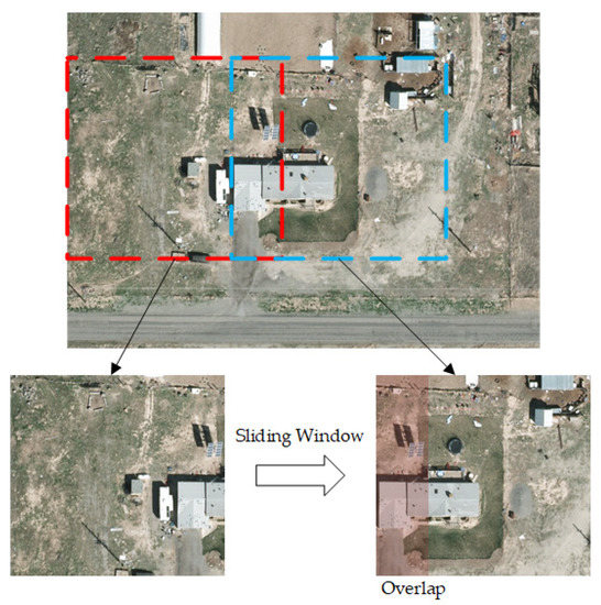
Figure 3.
Training sample clipping by sliding window in remote sensing images.
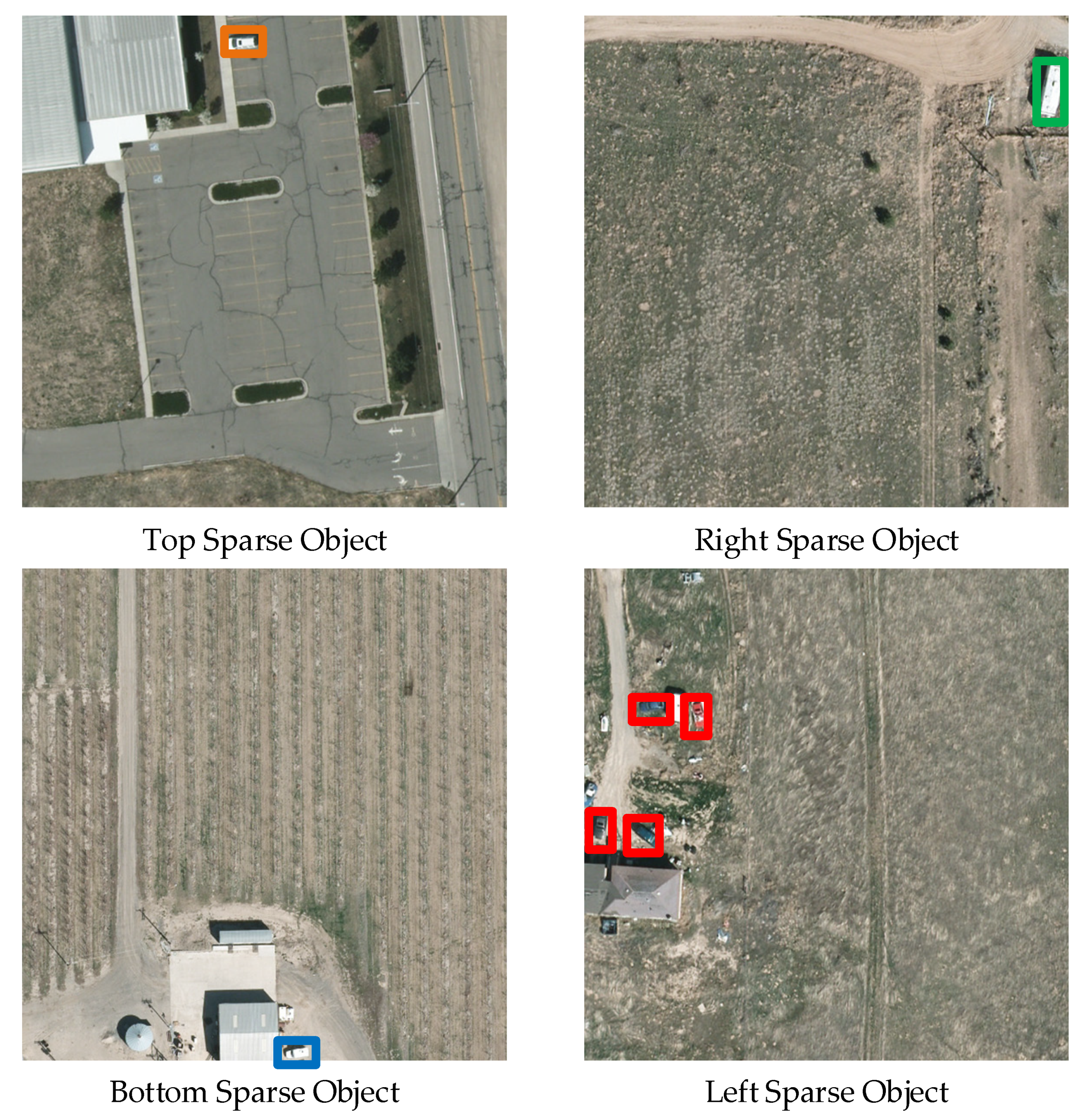
Remote sensing images often contain sparsely distributed objects that appear at low frequencies, particularly objects in deserted areas. Multiple sample fusion methods, such as Mosaic augmentation, may generate blank training samples (Figure 2). In the current paper, we reviewed an extensive number of satellite images to define the sparse object distribution as the objects cluster on the four corners or the four lines for the sliding images (Figure 4).
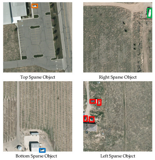
Figure 4.
Sparse object distribution.
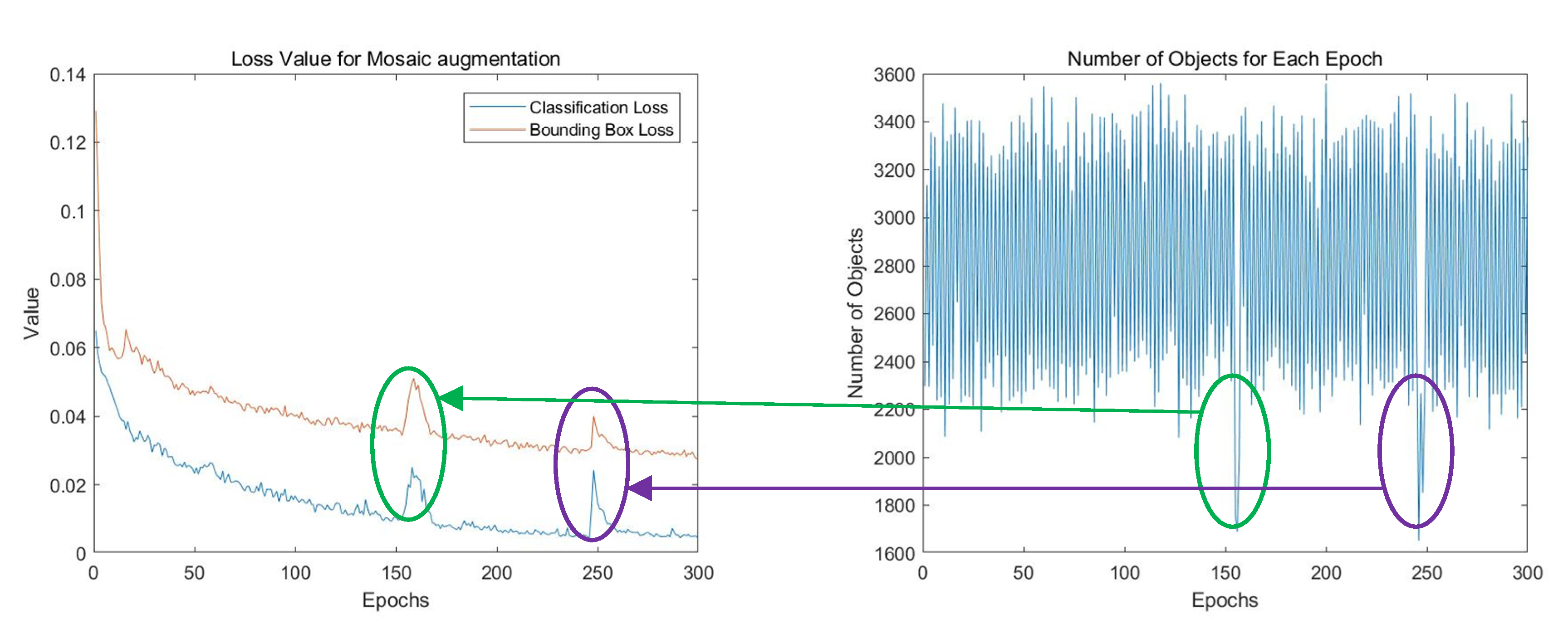
With more blank training samples generated, the instability of the number of objects in the training sample seriously disturbs the training process, resulting in an unsatisfactory performance. Figure 5 presents a training procedure and the number of objects in each training sample of the VEDAI dataset, a real remote sensing dataset with sparse object distributions. The number of objects vary greatly between training samples, leading to drastic classification, location losses, a slow convergence, and, ultimately, a poor performance.
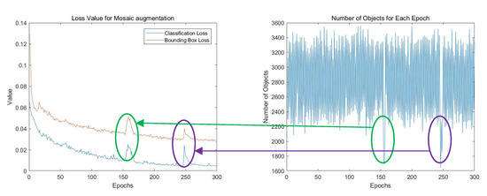
Figure 5.
Sparse object dataset leads to unstable training procedure.
3.2. Aggregated-Mosaic
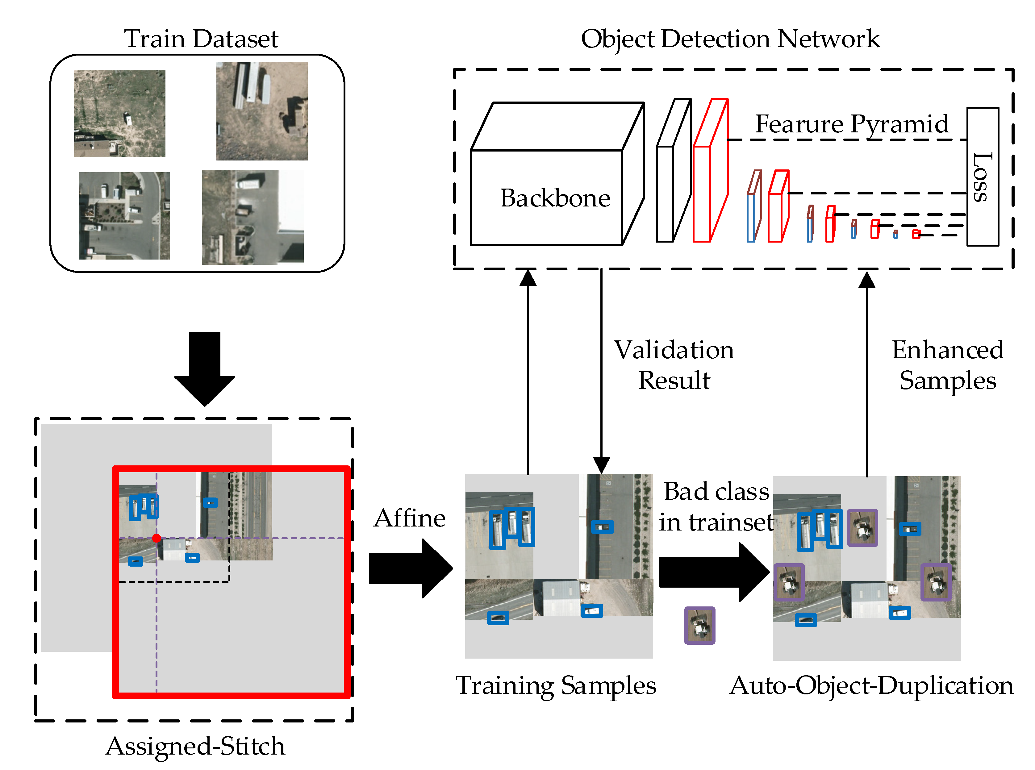
The proposed Aggregated-Mosaic is centered on the data augmentation procedure and contains two modules, Assigned-Stitch and Auto-Target-Duplication. Figure 6 depicts the implementation of the proposed algorithm. The first augmentation step, Assigned-Stitch, focuses on sparse objects. The Assigned-Stitch module requires that each training sample contain at least one object for a smooth training procedure. Auto-Target-Duplication focuses on classes that have generated poor results. Various copies of such classes are pasted on the training sample generated from the Assigned-Stitch module. This duplication procedure is not only a copy-paste strategy, but also a feedback strategy that can solve the sample imbalance and overfitting problems.

Figure 6.
Aggregated-Mosaic architecture.
3.3. Assigned-Stitch
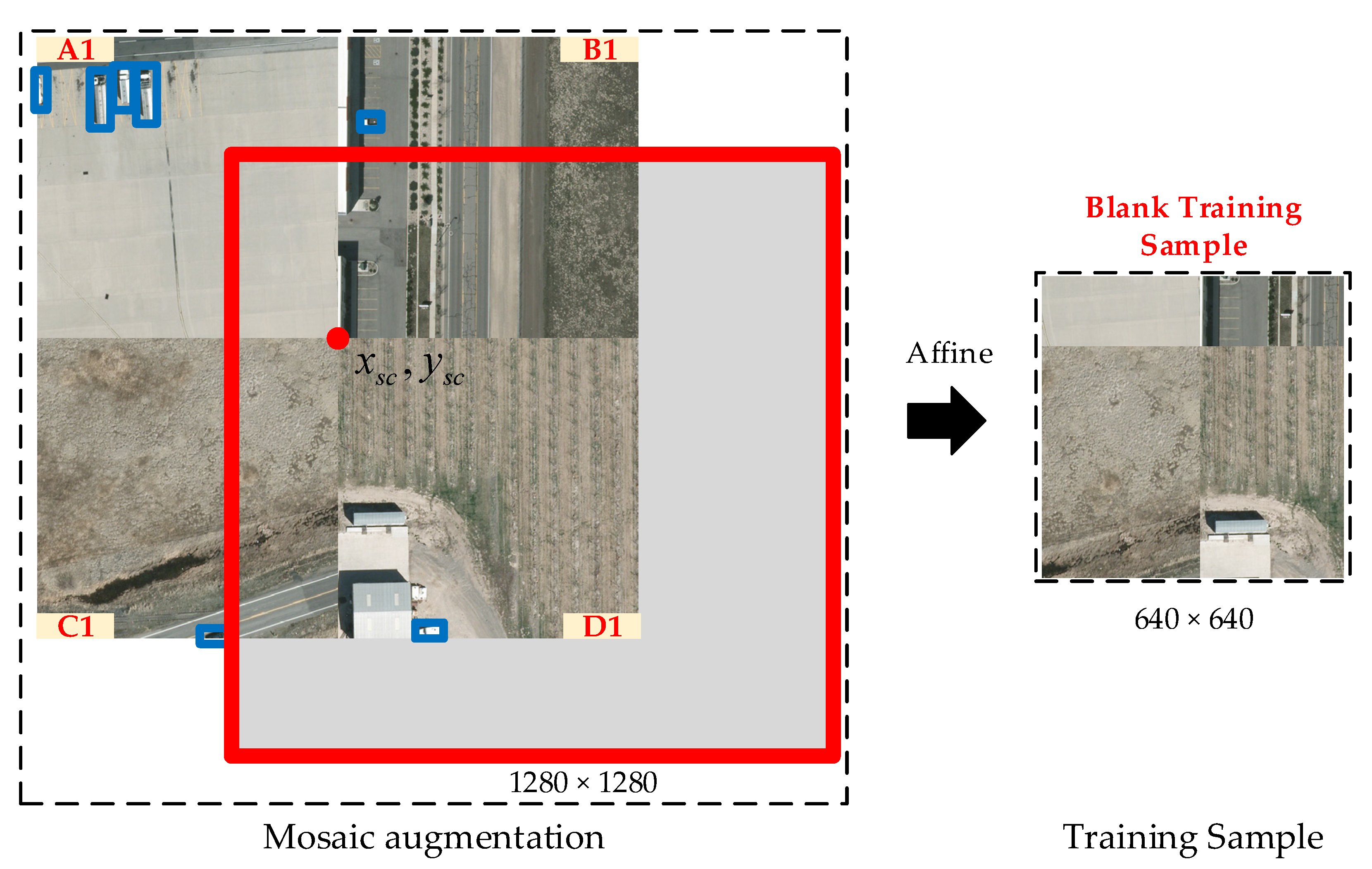
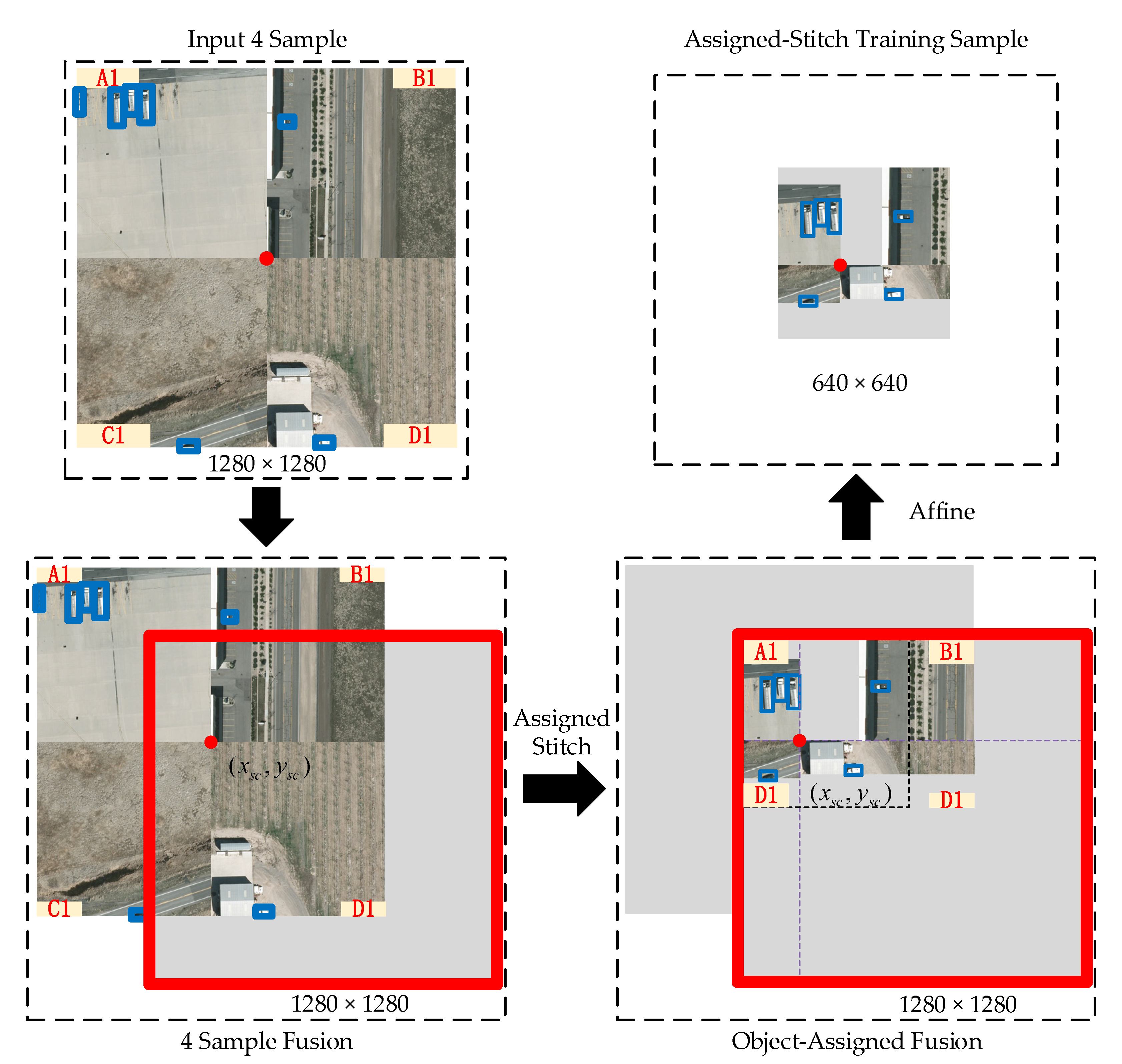
Considering that the objects in remote sensing images are often sparsely distributed, the traditional training sample generation methods will randomly generate blank samples, which only consist of backgrounds and make the training procedure is unstable. The Assigned-Stitch module constrains the objects in the sample by calculating the object locations and centers of the training sample slice. Figure 7 presents the Assigned-Stitch process flow. First, the dataloader module randomly selects four 640 × 640 samples (A1, B1, C1, and D1) for augmentation. These four samples are merged as a 1280 × 1280 image. Following the application of Mosaic, a 1280 × 1280 grey image is initialized, and the merged sample (with center (xsc, ysc)) is randomly placed on this grey image. Third, the Assigned-Stitch guarantees the distribution of the objects on the top-left of the fusion image, denoted as the Assigned-Object sample. Last, the affine transformation is applied on the Assigned-Object sample, and the top-left 640 × 640 section is sliced as the Assigned-Stitch training sample.
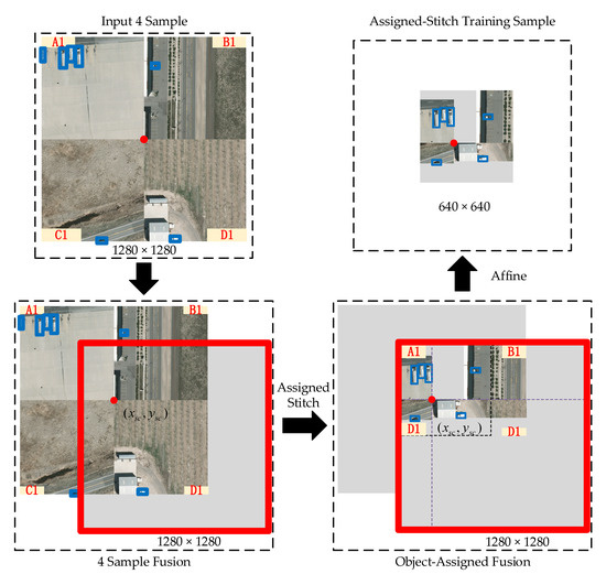
Figure 7.
Assigned-Stitch process flow.
In order to explain the Assigned-Stitch in detail, we select image A1 as an example. Figure 8 depicts the detailed Assigned-Stitch for A1.
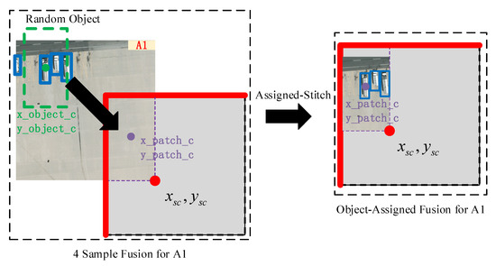
Figure 8.
Assigned-Stitch for A1 image.
In Figure 8, the purple rectangle denotes the location of the A1 sample, with center (x_patch_c, y_patch_c). Following this, an object in A1 is randomly selected (green rectangle) with center (x_object_c, y_object_c). Note that the green rectangle has the same area as the purple rectangle. The initial step of the Assigned-Stitch involves moving the green rectangle to the purple rectangle, ensuring that the fusion sample contains objects. Second, affine transformations (e.g., translation, rotation, and scaling) are applied on the object-assigned fusion samples. Based on the affine matrix, the ground truth is subjected to the same affine transformation, and the top-left 640 × 640 image must contain the affine ground truth. Algorithm 1 details the Assigned-Stitch procedure.
| Algorithm 1. Assigned-Stitch |
| Input: randomly select four images (A1, B1, C1, and D1) with w × h resolution; random object ground truth (g1’, g2’, g3’, g4’). Output: Assigned-Stitch training sample Ifu. 1 Initialize grey image Igrey, which value is 127 and Randomly select the slice center (xsc, ysc). 2 Purple rectangles for Igrey: Top-left: [xpmin1, ypmin1, xpmax1, ypmax1] = [max(xsc − w, 0), max(ysc − h, 0), xsc, ysc] Top-right: [xpmin2, ypmin2, xpmax2, ypmax2] = [ xsc, max(ysc − h, 0), max(xsc + w, w × 2), ysc] Bottom-left: [xpmin3, ypmin3, xpmax3, ypmax3] = [ max(xsc − w, 0), ysc, xsc, min(ysc + h, h × 2)] Bottom-right: [xpmin4, ypmin4, xpmax4, ypmax4] = [ xsc, ysc, min(xsc + w, w × 2), min(ysc + h, h × 2)] 3 Four input images slices (green rectangles) for each purple rectangle i: [xgmini, ygmini, xgmaxi, ygmaxi] = toRect([gxci’, gyci’, (xpmaxi − xpmini), (ypmaxi − ypmini)]) 4 Verify each image slices: if xgmini < 0, [xgmini, xgmaxi] = [0, (xpmaxi − xpmini)] if ygmini < 0, [ygmini, ygmaxi] = [0, (ypmaxi − ypmini)] if xgmaxi > w, [xgmini, xgmaxi] = [w − (xpmaxi - xpmini), w] if ygmaxi > h, [ygmini, ygmaxi] = [h − (ypmaxi − ypmini), h] 5 Place the image slices on Igrey: Igrey(xpmini:ypmini, xpmaxi:ypmaxi) = (xgmini:ygmini:xgmaxi:ygmaxi), i ∈ (1, 2, 3, 4) 6 Perform affine transformation: Repeat gi = affine(gi’, AffineMatrix) until the top-left w × h image contains objects. 7 Assigned-Stitch training sample: Ifu = affine(Igrey, AffineMatrix)(0:w, 0:h) |
In Algorithm 1, (xpmini, ypmini, xpmaxi, ypmaxi) denote the bounding box of the four corners i ∈ (1, 2, 3, 4) in grey image Igrey. (xgci, ygci, wgi, hgi), and (xgmini, ygmini, xgmaxi, ygmaxi) are the center and rectangle forms of the image slices. The toRect transform the center form to rectangle form and the function is as below:
where the (xc, yc, wc, hc) and (xmin, ymin, xmax, ymax) are center and rectangle forms, respectively. Thus, we ensure that the training samples of remote sensing images with sparse object distributions will contain objects.
xmin = xc − 0.5 × wc xmax = xc + 0.5 × wc
ymin = yc − 0.5 × hc ymax = yc + 0.5 × hc
ymin = yc − 0.5 × hc ymax = yc + 0.5 × hc
3.4. Auto-Target-Duplication
The sparse object distribution generally results in a class imbalance and hence complicates the detection results within the same level. The Auto-Target-Duplication module copies the objects of unsatisfactory class and thus forces the network pay more attention on this class. Figure 9 presents the Auto-Target-Duplication pipeline of the proposed Aggregated-Mosaic method.
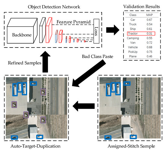
Figure 9.
Auto-Target-Duplication module.
Following “Copy-Paste” [53], a certain class with unsatisfactory results will be chosen to duplicate. In order to make the detection network pay more attention to the class with poor results, the validation dataset is evaluated after the training of each epoch, and the class with a 0.2 mean Average Precision (mAP) lower than the best class with highest mAP is selected as the unsatisfactory class. Objects of this class are randomly selected from the training set and pasted onto the Assigned-Stitch samples. This flow is a feedback procedure and forces the object detection network to pay more attention to the unsatisfactory class. Algorithm 2 details the Auto-Target-Duplication procedure.
| Algorithm 2. Auto-Target-Duplication |
| Input: detection network net(), training samples and ground truth for this epoch (img, label), results of validation dataset from last training model result. Output: Auto-Target-Duplication samples for this epoch (imgA, labelA). Repeat epochs: 1 Generate the Assigned-Stitch samples: (imgA, labelA) = AS(img, label) 2 Sort results and identify class with lowest result: classl = min(result) 3 Randomly select multiple objects for classl from training dataset: (obji, labeli), i = 1, 2, 3… 4 Duplicate (obji, labeli) to each Assigned-Stitch samples: (imgA, labelA) = Duplicate(imgA, labelA, obji, labeli), i = 1, 2, 3… 5 Use Assigned-Stitch samples to train the detection network in each iteration: net = train(net(), imgA, labelA) |
Testing the validation dataset from the last training model determines the class with lowest result and the (obji, labeli) of this class is duplicated on the Assigned-Stitch samples. The detection network is trained on the Auto-Target-Duplication samples. In contrast to traditional copy-paste methods, the Auto-Target-Duplication is a feedback procedure and could make the detection network pay more attention to the class with the lowest result.
4. Experiment
In this section, we choose VEADI and NWPU VHR-10 datasets, which are two real remote sensing datasets and contain the objects with sparse distribution, to evaluate the proposed method. Then, the training settings and discussions are explained in detail.
4.1. Datasets
4.1.1. VEDAI
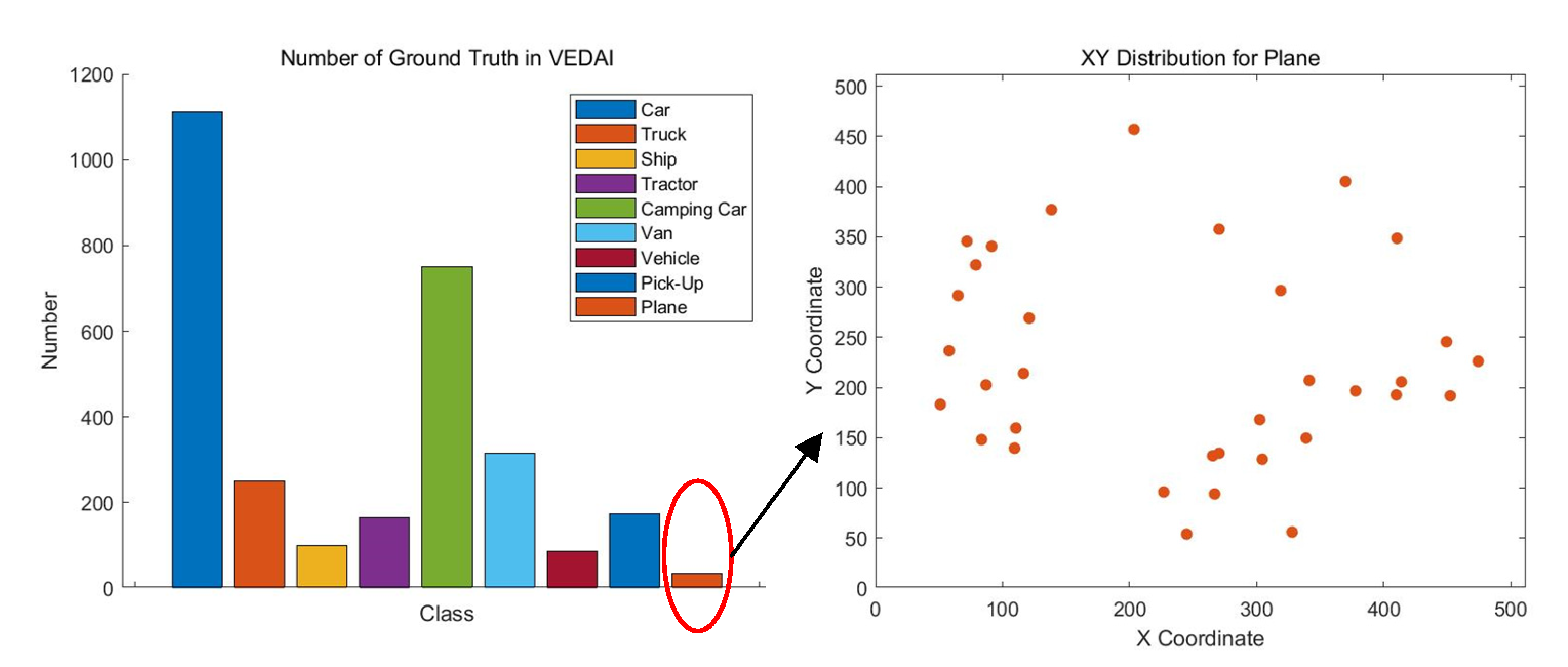
VEDAI [54] contains two subsets: (i) VEDAI_512 includes 1268 RGB tiles (512 × 512) and the associated infrared (IR) images at a 0.25 m spatial resolution; and (ii) VEDAI_1024 compromises 1268 RGB tiles (1024 × 1024) and the associated infrared (IR) images at a 0.125 m spatial resolution. For each tile, annotations with nine classes (Car, Truck, Ship, Tractor, Camping Car, Van, Vehicle, Pick-Up, and Plane) are provided with bounding boxes in the image. We choose this dataset for its sparse object distribution. The images of VEDAI_1024 dataset are sliced to a size of 640 × 640 with 256 strides and images with no objects are deleted. Figure 10 depicts the number of objects in VEDAI and the XY distribution for the Plane class and its sparse distribution.

Figure 10.
XY distribution for the Plane class in the VEDAI dataset.
4.1.2. NWPU VHR-10
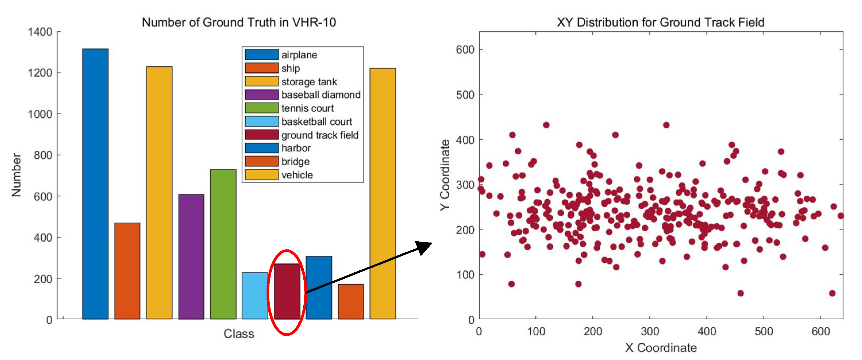
The NWPU VHR-10 [55] dataset contains 10 geospatial object classes including airplane (PL), baseball diamond (BD), basketball court (BC), bridge, harbor (BH), ground track field (GT), ship (SH), storage tank (ST), tennis court (TC), and vehicle (VH). It consists of 715 RGB images and 85 pan-sharpened color infrared images. The 715 RGB images are collected from Google Earth and their spatial resolutions vary from 0.5 m to 2 m. The 85 pan-sharpened infrared images, with a spatial resolution of 0.08 m, are obtained from Vaihingen data. This dataset contains a total of 3775 object instances that are manually annotated with horizontal bounding boxes. The training and testing sets are randomly selected, and contain 520 and 130 images, respectively. As with VEDAI_1024, the images are sliced to a size of 640 × 640 with 256 strides and images with no objects are deleted. Figure 11 presents the number of objects in VHR-10 and the XY distribution for the Ground Track Field class of the dataset and the distribution of it is sparse obviously. Based on the explanation in Section 3.1, multiple sample fusion methods, such as Mosaic augmentation, may generate blank training samples, and the instability of the number of objects in the training sample seriously disturbs the training process, resulting in an unsatisfactory performance.

Figure 11.
XY distribution for the Ground Track Field class of the NWPU VHR-10 dataset.
4.2. Training Settings
We employ Mosaic (YOLOv5) as the baseline method, and the majority of settings are equal to those of Yolov5.
4.2.1. Anchor Generation
The anchor size for each dataset is generated via K-means clustering, which is adopted to restrain the anchors in Yolov5. The following is the function of K-means, which minimizes the clustering centers and each ground truths.
where E is the objective function. Ci is the clustering settings, which contain ground truths x. The x is composed of (w, h) for each ground truths. k is the number of clustering centers; in this experiment, k is 9. Finally, μi is the clustering centers, which is also anchor shapes.
The anchor shapes are generated by clustering the shapes of the ground truths and employing genetic evolution with the actual training loss criteria used during training. Table 1 reports the anchor shapes for each dataset. The detection procedure is applied on the P3, P4, and P5 feature maps and the detection area is subsequently increased. For the VEDAI_512 dataset, the anchors shapes (w, h) are (27,11) (13,27) (27,18) for P3, (22,25) (17,43) (46,17) for P4, and (35,32) (33,78) (82,70) for P5. For the VEDAI_1024 dataset, the anchors shapes are (35,34) (25,54) (47,52) for P3, (64,40) (70,63) (55,92) for P4, and (87,83) (152,110) (210,248) for P5. All anchor shapes are detailed in Table 1.

Table 1.
Anchor shapes for each feature map.
4.2.2. Learning Policy
For each dataset, the network is warmed up by a learning rate of 10−4 for 10 epochs. The initial learning rate is 0.01 and we used the cosine annealing of 0.012 to reduce the learning rate step by step. The optimization trick has a momentum of 0.9 and a weight decay of 0.0005. We employed the CIoU and GIoU [30,31] loss functions for the bounding box regression and classification, respectively.
4.3. Experiment Results
In this section, we evaluate Aggregated-Mosaic for its capability to improve the object detection performance compared to other current methods. All experiments were implemented and evaluated on the Pytorch framework. We compared the proposed method with the Basic [21], CutOut [37], GridMask [56,57], MixUp [12], CutMix [11], and Mosaic [28] augmentation methods. The Mosaic augmentation method is the baseline of the proposed method. Following the SSD settings, Basic represents the basic data augmentation (e.g., horizontal flip, random sample, and color distortion). Hyper-parameter α is equal to 0.5 for MixUp and CutMix, while the hyper-parameter p of GridMask is 0.7. We adopted Soft-NMS to accurately fix the candidate bounding boxes.
4.3.1. VEDAI 512
Table 2 reports the mAP results on the VEDAI_512 validation dataset. Bold values denote the best performances. From the table, the baseline Mosaic achieves a mAP of 68.49%, while our proposed method achieves 71.21%, which is a 2.72% improvement compared to the baseline. Moreover, compared with the recent data augmentation methods (Basic, CutOut, GridMask, MixUp, and CutMix), the proposed Aggregated-Mosaic method achieves the best performance.
Table 2.
Results of VEDAI 512.
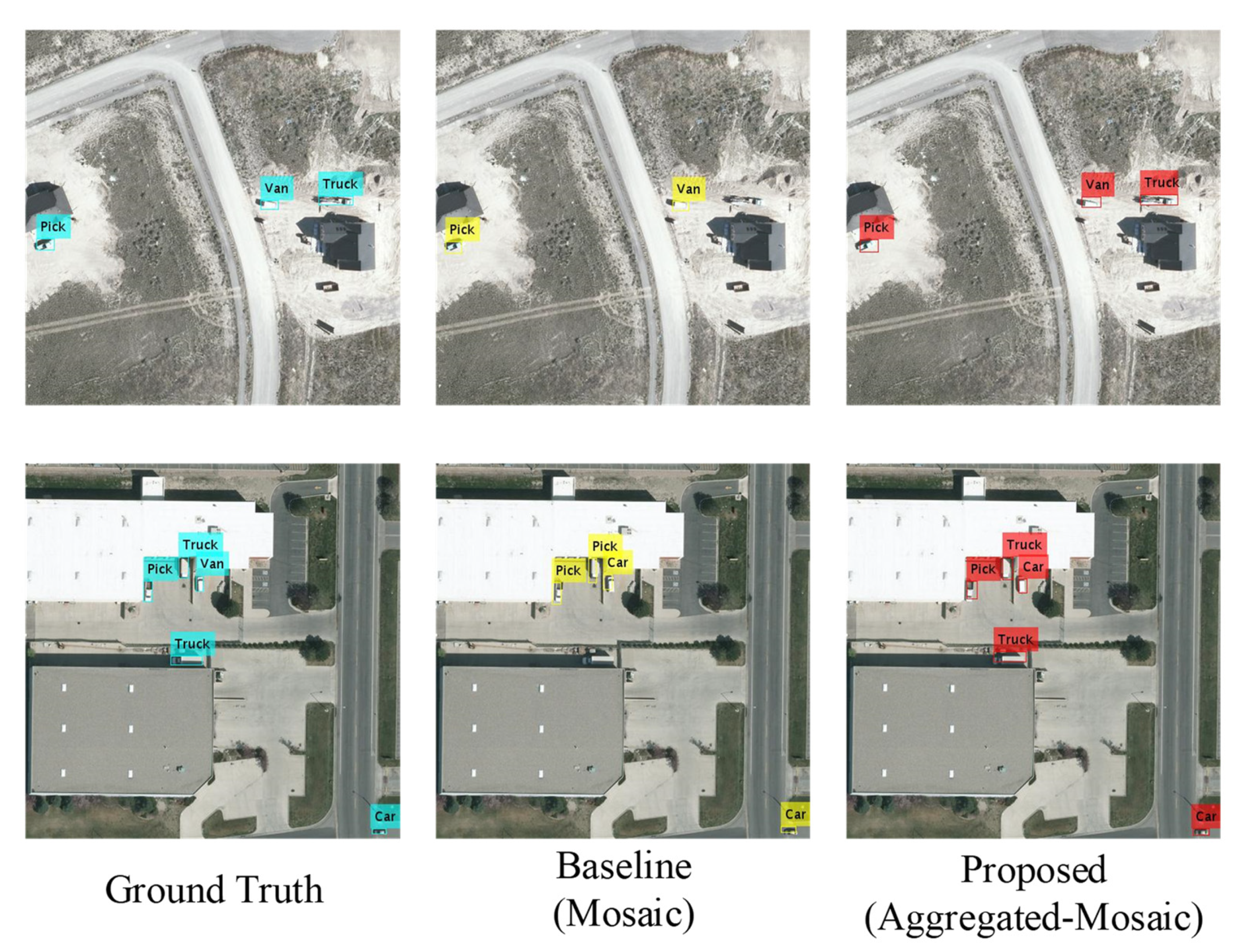
Figure 12 shows the detection results in VEDAI 512 dataset.
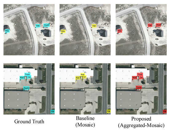
Figure 12.
Detection result: Ground Truth (right), Mosaic (middle), Aggregated-Mosaic (left).
4.3.2. VEDAI 1024
Table 3 reports the mAP results on the VEDAI_1024 validation dataset. Bold values denote the best performances. From the table, the baseline Mosaic achieves a mAP of 71.38%, while our proposed method achieves 76.82%, which is a 5.44% improvement compared to the baseline. Moreover, compared with the recent data augmentation methods (Basic, CutOut, GridMask, MixUp, and CutMix), the proposed Aggregated-Mosaic method achieves the best performance.
Table 3.
Results of VEDAI 1024.
Figure 13 shows the detection results in VEDAI 1024 dataset.
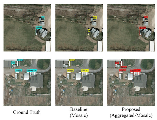
Figure 13.
Detection result: Ground Truth (right), Mosaic (middle), Aggregated-Mosaic (left).
4.3.3. NWPU-VHR 10
Table 4 reports the mAP results on the NWPU-VHR 10 validation dataset. Bold values denote the best performances. From the table, the baseline Mosaic achieves a mAP of 90.64%, while our proposed method achieves 96.12%, which is a 5.48% improvement compared to the baseline. Moreover, compared with the recent data augmentation methods (Basic, CutOut, GridMask, MixUp, and CutMix), the proposed Aggregated-Mosaic method achieves the best performance.
Table 4.
Results of NWPU-VHR 10.
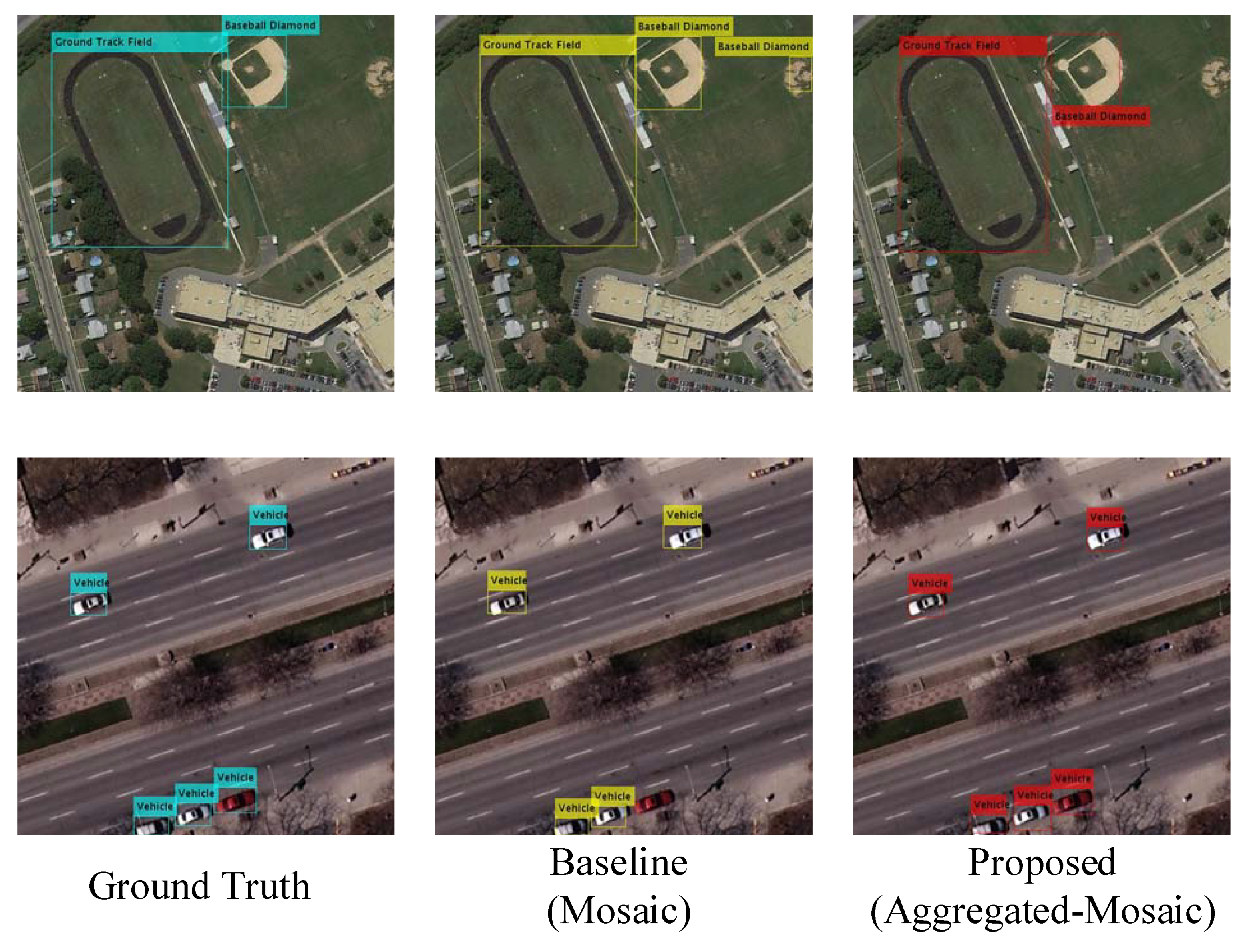
Figure 14 shows the detection results in NWPU-VHR 10 dataset.
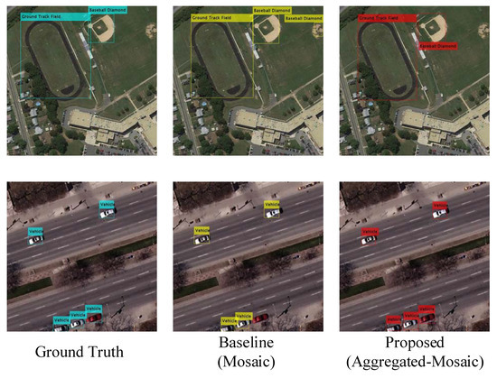
Figure 14.
Detection result: Ground Truth (right), Mosaic (middle), Aggregated-Mosaic (left).
4.4. Disscussion
From the experiment results, the proposed method fails to achieve the best results in some types of objects. The main reason is that if the objects are not distributed sparsely, the proposed method has a similar effect compared with the basic or sample fusion methods. Then, due to the Auto-Target-Duplication module, the training procedure will distract from those types of objects, and could not get the best result. Considering the influence of the hyper-parameter, we conducted an ablation study for Aggregated-Mosaic. The Assigned-Stitch component of the proposed method does not include any hyper-parameters in the augmentation procedure, while the Auto-Target-Duplication contains a hyper-parameter equal to the object duplication times. Thus, we perform an additional experiment that evaluates the effects of duplication times and gaussian blur on the three datasets based on the following.
X1: In Algorithm 2, randomly select one object for classl from the training data and duplicate this to the Assigned-Stitch sample.
X5: In Algorithm 2, randomly select five objects for classl from the training data and duplicate them to the Assigned-Stitch sample.
X10: In Algorithm 2, randomly select ten objects for classl from the training data and duplicate them to the Assigned-Stitch sample.
Gaussian blur: When the object is duplicated to the Assigned-Stitch sample, the edge of the object patch is smoothed by Gaussian blurring (0 and 1 mean and variance, respectively) to the Assigned-Stitch sample.
Table 5 reveals that the Gaussian edge blur does not improve the detection performance, and thus the sharp edges of the object patch are better than the smoothed edges. In addition, the performance is optimized for the duplication times of 5 or 10.
Table 5.
Ablation study for the duplication times and Gaussian blur.
5. Conclusions
In this paper, for training the object detection network in remote sensing imagery with sparse object distributions, we propose the Aggregated-Mosaic object detection method, which includes the Assigned-Stitch and Auto-Target-Duplication modules. The main improvements consist of two parts: (1) Based on the ground truth and Mosaic image sizes, the Assigned-Stitch augmentation enhances each training sample by accounting for objects, thus ensuring an efficient training procedure. (2) Objects are then carefully selected for duplication, and the Auto-Target-Duplication solves the sample imbalance, particularly for classes with poor results. The proposed method is evaluated with three remote sensing datasets, outperforming Mosaic (YOLOv5) by 2.72% and 5.44% at the 512 × 512 and 1024 × 1024 resolutions of the VEDAI dataset, respectively. Furthermore, on the VHR-10 dataset, the proposed method outperforms Mosaic (YOLOv5) by 5.48%. In future work, for the problem of lacking training samples, the proposed method will be combined with Generative Adversarial Networks to improve the detection performance for remote sensing imagery.
Author Contributions
B.Z. (Boya Zhao) and Y.W. created and designed the framework. B.Z. (Boya Zhao) and X.G. performed the algorithm on Pytorch. B.Z. (Boya Zhao), Y.W., L.G. and B.Z. (Bing Zhang) wrote the paper. All authors have read and agreed to the published version of the manuscript.
Funding
This research was funded by National Natural Science Foundation of China, grant number 62001455 and 41871245.
Institutional Review Board Statement
Not applicable.
Informed Consent Statement
Not applicable.
Data Availability Statement
Not applicable.
Conflicts of Interest
The authors declare no conflict of interest.
References
- Hong, D.; Yokoya, N.; Xia, G.-S.; Chanussot, J.; Zhu, X.X. X-ModalNet: A semi-supervised deep cross-modal network for classification of remote sensing data. ISPRS J. Photogramm. Remote Sens. 2020, 167, 12–23. [Google Scholar] [CrossRef]
- Hou, J.-B.; Zhu, X.; Yin, X.-C. Self-Adaptive Aspect Ratio Anchor for Oriented Object Detection in Remote Sensing Images. Remote Sens. 2021, 13, 1318. [Google Scholar] [CrossRef]
- Wu, X.; Hong, D.; Chanussot, J.; Xu, Y.; Tao, R.; Wang, Y. Fourier-based rotation-invariant feature boosting: An efficient framework for geospatial object detection. IEEE Geosci. Remote Sens. Lett. 2019, 17, 302–306. [Google Scholar] [CrossRef] [Green Version]
- Awad, M.M.; Lauteri, M. Self-Organizing Deep Learning (SO-UNet)—A Novel Framework to Classify Urban and Peri-Urban Forests. Sustainability 2021, 13, 5548. [Google Scholar] [CrossRef]
- Shorten, C.; Khoshgoftaar, T.M. A survey on image data augmentation for deep learning. J. Big Data 2019, 6, 1–48. [Google Scholar] [CrossRef]
- Nusrat, I.; Jang, S.-B. A comparison of regularization techniques in deep neural networks. Symmetry 2018, 10, 648. [Google Scholar] [CrossRef] [Green Version]
- Dalal, N.; Triggs, B. Histograms of oriented gradients for human detection. In Proceedings of the IEEE Conference on Computer Vision and Pattern Recognition (CVPR), San Diego, CA, USA, 20–25 June 2005; pp. 886–893. [Google Scholar]
- Yan, J.; Lei, Z.; Wen, L.; Li, S.Z. The fastest deformable part model for object detection. In Proceedings of the IEEE Conference on Computer Vision and Pattern Recognition (CVPR), Columbus, OH, USA, 24–27 June 2014; pp. 2497–2504. [Google Scholar]
- Cao, J.; Cholakkal, H.; Anwer, R.M.; Khan, F.S.; Pang, Y.; Shao, L. D2det: Towards high quality object detection and instance segmentation. In Proceedings of the IEEE Conference on Computer Vision and Pattern Recognition (CVPR), Seattle, WA, USA, 14–19 June 2020; pp. 11485–11494. [Google Scholar]
- He, K.; Gkioxari, G.; Dollár, P.; Girshick, R. Mask R-CNN. In Proceedings of the IEEE Conference on Computer Vision and Pattern Recognition (CVPR), Honolulu, HI, USA, 16–21 July 2017; pp. 2961–2969. [Google Scholar]
- Yun, S.; Han, D.; Oh, S.J.; Chun, S.; Choe, J.; Yoo, Y. Cutmix: Regularization strategy to train strong classifiers with localizable features. In Proceedings of the IEEE International Conference on Computer Vision (ICCV), Seoul, Korea, 27 October–2 November 2019; pp. 6023–6032. [Google Scholar]
- Zhang, H.; Cisse, M.; Dauphin, Y.N.; Lopez-Paz, D. Mixup: Beyond empirical risk minimization. In Proceedings of the 6th International Conference on Learning Representations (ICLR), Vancouver, BC, Canada, 30 April–3 May 2018. [Google Scholar]
- Ultralytics. YOLOv5. Available online: https://github.com/ultralytics/yolov5 (accessed on 8 May 2021).
- Lowe, D.G. Distinctive image features from scale-invariant keypoints. Int. J. Comput. Vis. 2004, 60, 91–110. [Google Scholar] [CrossRef]
- Rätsch, G.; Onoda, T.; Müller, K.-R. Soft margins for AdaBoost. Mach. Learn. 2001, 42, 287–320. [Google Scholar] [CrossRef]
- Suykens, J.A.; Vandewalle, J. Least squares support vector machine classifiers. Neural Process. Lett. 1999, 9, 293–300. [Google Scholar] [CrossRef]
- Felzenszwalb, P.; McAllester, D.; Ramanan, D. A discriminatively trained, multiscale, deformable part model. In Proceedings of the IEEE Conference on Computer Vision and Pattern Recognition (CVPR), Anchorage, AK, USA, 24–26 June 2008; pp. 1–8. [Google Scholar]
- Russakovsky, O.; Deng, J.; Su, H.; Krause, J.; Satheesh, S.; Ma, S.; Huang, Z.; Karpathy, A.; Khosla, A.; Bernstein, M. Imagenet large scale visual recognition challenge. Int. J. Comput. Vis. 2015, 115, 211–252. [Google Scholar] [CrossRef] [Green Version]
- Krizhevsky, A.; Sutskever, I.; Hinton, G.E. Imagenet classification with deep convolutional neural networks. In Proceedings of the Advances in Neural Information Processing Systems (NIPS), Lake Tahoe, NV, USA, 3–6 December 2012; pp. 1097–1105. [Google Scholar]
- Redmon, J.; Divvala, S.; Girshick, R.; Farhadi, A. You only look once: Unified, real-time object detection. In Proceedings of the IEEE Conference on Computer Vision and Pattern Recognition (CVPR), Las Vegas, NV, USA, 27–30 June 2016; pp. 779–788. [Google Scholar]
- Liu, W.; Anguelov, D.; Erhan, D.; Szegedy, C.; Reed, S.; Fu, C.-Y.; Berg, A.C. Ssd: Single shot multibox detector. In Proceedings of the European Conference on Computer Vision (ECCV), Amsterdam, The Netherlands, 11–14 October 2016; pp. 21–37. [Google Scholar]
- Girshick, R.; Donahue, J.; Darrell, T.; Malik, J. Rich feature hierarchies for accurate object detection and semantic segmentation. In Proceedings of the IEEE Conference on Computer Vision and Pattern Recognition (CVPR), Columbus, OH, USA, 24–27 June 2014; pp. 580–587. [Google Scholar]
- Redmon, J.; Farhadi, A. YOLO9000: Better, faster, stronger. In Proceedings of the IEEE conference on Computer Vision and Pattern Recognition (CVPR), Honolulu, HI, USA, 16–21 July 2017; pp. 7263–7271. [Google Scholar]
- Redmon, J.; Farhadi, A. Yolov3: An incremental improvement. arXiv 2018, arXiv:1804.02767. [Google Scholar]
- Choi, J.; Chun, D.; Kim, H.; Lee, H.-J. Gaussian yolov3: An accurate and fast object detector using localization uncertainty for autonomous driving. In Proceedings of the IEEE International Conference on Computer Vision (ICCV), Seoul, Korea, 27 October–2 November 2019; pp. 502–511. [Google Scholar]
- Lin, T.-Y.; Dollár, P.; Girshick, R.; He, K.; Hariharan, B.; Belongie, S. Feature pyramid networks for object detection. In Proceedings of the IEEE Conference on Computer Vision and Pattern Recognition (CVPR), Honolulu, HI, USA, 16–21 July 2017; pp. 2117–2125. [Google Scholar]
- Girshick, R. Fast R-CNN. In Proceedings of the IEEE International Conference on Computer Vision (ICCV), Santiago, Chile, 7–13 December 2015; pp. 1440–1448. [Google Scholar]
- Bochkovskiy, A.; Wang, C.-Y.; Liao, H.-Y.M. Yolov4: Optimal speed and accuracy of object detection. arXiv 2020, arXiv:2004.10934. [Google Scholar]
- Wang, C.-Y.; Bochkovskiy, A.; Liao, H.-Y.M. Scaled-yolov4: Scaling cross stage partial network. In Proceedings of the IEEE Conference on Computer Vision and Pattern Recognition (CVPR), Virtual, 19–25 June 2021; pp. 13029–13038. [Google Scholar]
- Zheng, Z.; Wang, P.; Ren, D.; Liu, W.; Ye, R.; Hu, Q.; Zuo, W. Enhancing geometric factors in model learning and inference for object detection and instance segmentation. arXiv 2020, arXiv:2005.03572. [Google Scholar]
- Zheng, Z.; Wang, P.; Liu, W.; Li, J.; Ye, R.; Ren, D. Distance-IoU loss: Faster and better learning for bounding box regression. In Proceedings of the AAAI Conference on Artificial Intelligence, New York, NY, USA, 7–12 February 2020; pp. 12993–13000. [Google Scholar]
- Ren, S.; He, K.; Girshick, R.; Sun, J. Faster R-CNN: Towards real-time object detection with region proposal networks. IEEE Trans. Pattern Anal. Mach. Intell. 2016, 39, 1137–1149. [Google Scholar] [CrossRef] [PubMed] [Green Version]
- Duan, K.; Bai, S.; Xie, L.; Qi, H.; Huang, Q.; Tian, Q. Centernet: Keypoint triplets for object detection. In Proceedings of the IEEE International Conference on Computer Vision (ICCV), Seoul, Korea, 27 October–2 November 2019; pp. 6569–6578. [Google Scholar]
- Ghiasi, G.; Lin, T.-Y.; Le, Q.V. Dropblock: A regularization method for convolutional networks. In Proceedings of the Advances in Neural Information Processing Systems (NIPS), Montréal, QC, Canada, 3–8 December 2018; pp. 10750–10760. [Google Scholar]
- Srivastava, N.; Hinton, G.; Krizhevsky, A.; Sutskever, I.; Salakhutdinov, R. Dropout: A simple way to prevent neural networks from overfitting. J. Mach. Learn. Res. 2014, 15, 1929–1958. [Google Scholar]
- Zhong, Z.; Zheng, L.; Kang, G.; Li, S.; Yang, Y. Random erasing data augmentation. In Proceedings of the AAAI Conference on Artificial Intelligence, New York, NY, USA, 7–12 February 2020; pp. 13001–13008. [Google Scholar]
- DeVries, T.; Taylor, G.W. Improved regularization of convolutional neural networks with cutout. arXiv 2017, arXiv:1708.04552. [Google Scholar]
- Real, E.; Aggarwal, A.; Huang, Y.; Le, Q.V. Regularized evolution for image classifier architecture search. In Proceedings of the AAAI Conference on Artificial Intelligence, Honolulu, HI, USA, 27 January–1 February 2019; pp. 4780–4789. [Google Scholar]
- Dwibedi, D.; Misra, I.; Hebert, M. Cut, paste and learn: Surprisingly easy synthesis for instance detection. In Proceedings of the IEEE International Conference on Computer Vision (ICCV), Venice, Italy, 22–29 October 2017; pp. 1301–1310. [Google Scholar]
- Dvornik, N.; Mairal, J.; Schmid, C. Modeling visual context is key to augmenting object detection datasets. In Proceedings of the European Conference on Computer Vision (ECCV), Munich, Germany, 8–14 September 2018; pp. 364–380. [Google Scholar]
- Geirhos, R.; Rubisch, P.; Michaelis, C.; Bethge, M.; Wichmann, F.A.; Brendel, W. ImageNet-trained CNNs are biased towards texture; increasing shape bias improves accuracy and robustness. In Proceedings of the 7th International Conference on Learning Representations (ICLR), New Orleans, LA, USA, 6–9 May 2019. [Google Scholar]
- Tokozume, Y.; Ushiku, Y.; Harada, T. Between-class learning for image classification. In Proceedings of the IEEE Conference on Computer Vision and Pattern Recognition (CVPR), 18–22 June 2018; pp. 5486–5494. [Google Scholar]
- Takahashi, R.; Matsubara, T.; Uehara, K. Data augmentation using random image cropping and patching for deep cnns. IEEE Trans. Circuits Syst. Video Technol. 2019, 30, 2917–2931. [Google Scholar] [CrossRef] [Green Version]
- Ioffe, S.; Szegedy, C. Batch normalization: Accelerating deep network training by reducing internal covariate shift. In Proceedings of the International Conference on Machine Learning (ICML), Lille, France, 6–11 July 2015; pp. 448–456. [Google Scholar]
- Kingma, D.P.; Ba, J. Adam: A method for stochastic optimization. In Proceedings of the 3rd International Conference on Learning Representations (ICLR), San Diego, CA, USA, 7–9 May 2015. [Google Scholar]
- Loshchilov, I.; Hutter, F. Decoupled weight decay regularization. In Proceedings of the 7th International Conference on Learning Representations (ICLR), New Orleans, LA, USA, 6–9 May 2019. [Google Scholar]
- Shafahi, A.; Najibi, M.; Xu, Z.; Dickerson, J.; Davis, L.S.; Goldstein, T. Universal adversarial training. In Proceedings of the AAAI Conference on Artificial Intelligence, New York, NY, USA, 7–12 February 2020; pp. 5636–5643. [Google Scholar]
- Wang, J.; Yang, Y.; Chen, Y.; Han, Y. LighterGAN: An Illumination Enhancement Method for Urban UAV Imagery. Remote Sens. 2021, 13, 1371. [Google Scholar] [CrossRef]
- Awad, M.M.; De Jong, K. Optimization of spectral signatures selection using multi-objective genetic algorithms. In Proceedings of the IEEE Congress of Evolutionary Computation (CEC), New Orleans, LA, USA, 5–8 June 2011; pp. 1620–1627. [Google Scholar]
- Ding, Y.; Zhou, Y.; Zhu, Y.; Ye, Q.; Jiao, J. Selective sparse sampling for fine-grained image recognition. In Proceedings of the IEEE International Conference on Computer Vision (ICCV), Seoul, Korea, 27 October–2 November 2019; pp. 6599–6608. [Google Scholar]
- Zheng, S.; Zhang, Y.; Liu, W.; Zou, Y. Improved image representation and sparse representation for image classification. Appl. Intell. 2020, 1–12. [Google Scholar] [CrossRef]
- Van Etten, A. You only look twice: Rapid multi-scale object detection in satellite imagery. arXiv 2018, arXiv:1805.09512. [Google Scholar]
- Ghiasi, G.; Cui, Y.; Srinivas, A.; Qian, R.; Lin, T.-Y.; Cubuk, E.D.; Le, Q.V.; Zoph, B. Simple copy-paste is a strong data augmentation method for instance segmentation. In Proceedings of the IEEE Conference on Computer Vision and Pattern Recognition (CVPR), Virtual, 19–25 June 2021; pp. 2918–2928. [Google Scholar]
- Razakarivony, S.; Jurie, F. Vehicle detection in aerial imagery: A small target detection benchmark. J. Vis. Commun. Image Represent. 2016, 34, 187–203. [Google Scholar] [CrossRef] [Green Version]
- Cheng, G.; Han, J. A survey on object detection in optical remote sensing images. ISPRS J. Photogramm. Remote Sens. 2016, 117, 11–28. [Google Scholar] [CrossRef] [Green Version]
- Chen, P.; Liu, S.; Zhao, H.; Jia, J. Gridmask data augmentation. arXiv 2020, arXiv:2001.04086. [Google Scholar]
- Wang, J.; Jin, S.; Liu, W.; Liu, W.; Qian, C.; Luo, P. When human pose estimation meets robustness: Adversarial algorithms and benchmarks. In Proceedings of the IEEE Conference on Computer Vision and Pattern Recognition (CVPR), Virtual, 19–25 June 2021; pp. 11855–11864. [Google Scholar]


Publisher’s Note: MDPI stays neutral with regard to jurisdictional claims in published maps and institutional affiliations. |
© 2021 by the authors. Licensee MDPI, Basel, Switzerland. This article is an open access article distributed under the terms and conditions of the Creative Commons Attribution (CC BY) license (https://creativecommons.org/licenses/by/4.0/).