
Development and Application of Earth Observation Based Machine Learning Methods for Characterizing Forest and Land Cover Change in Dilijan National Park of Armenia between 1991 and 2019

 ,
,
Abstract
:1. Introduction
1.1. Context
1.2. Aim and Objectives
2. Data
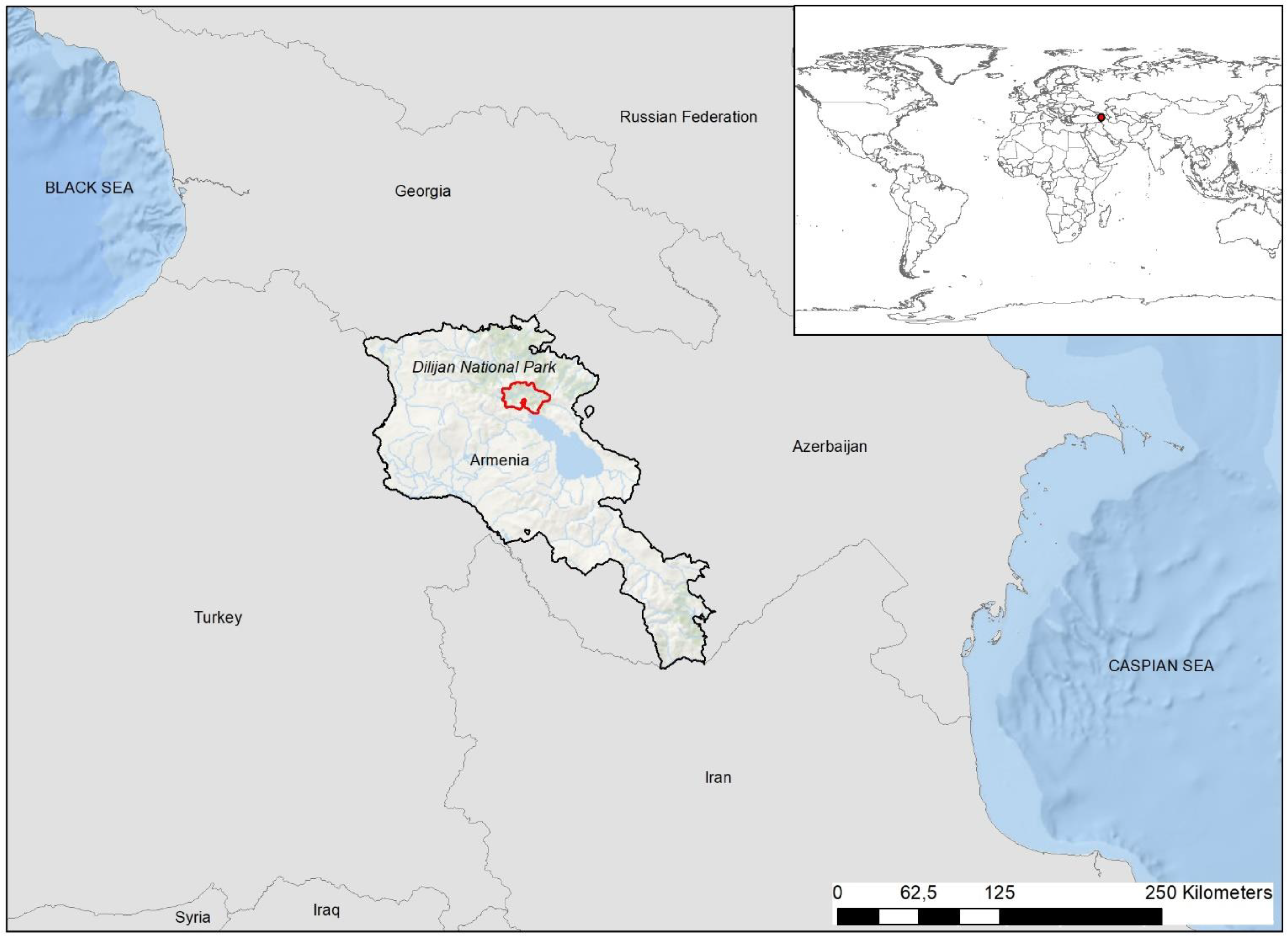
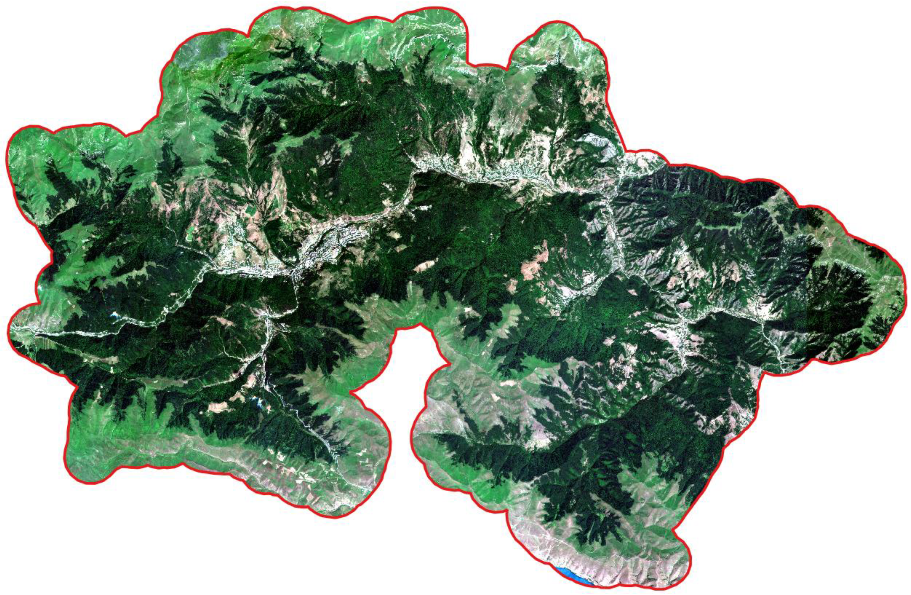
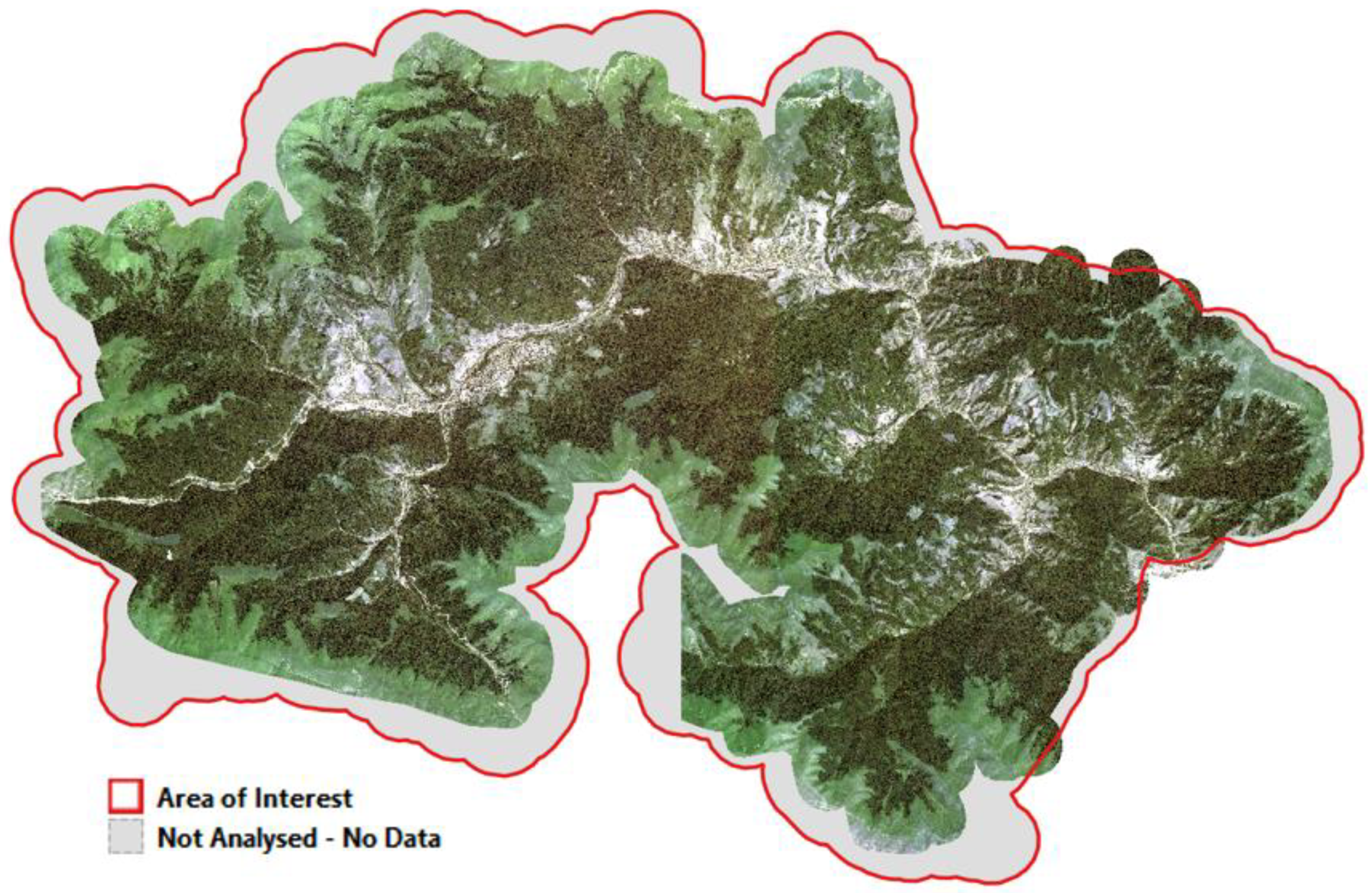
2.1. Study Area
2.2. In Situ Data
2.3. EO Data
- Ikonos at 4 m spatial resolution for the year 2007, used for epoch 2005
- Pléiades of 17 July 2014 and 24 July 2014 at 0.5 m resolution (Panchromatic) and 2 m (Multispectral) used for epoch 2015 (see Figure 3)
- Pléiades of 28 June 2018 at 0.5 m resolution (Panchromatic) and 2 m (Multispectral), used for epoch 2019.
Data Pre-Processing
3. Methods
3.1. Characterization of Forest Ecosystems
3.1.1. Specifications
3.1.2. Forest Mask
- (i)
- Pre-processing
- (ii)
- Classification of the Forest Mask
- (iii)
- Post-processing
- (iv)
- Computing of raw Forest Change Mask
- (v)
- Manual Enhancement of polygons of change
- (vi)
- Quality Check of the consistency of the Forest Masks and Forest Change Masks for all epochs
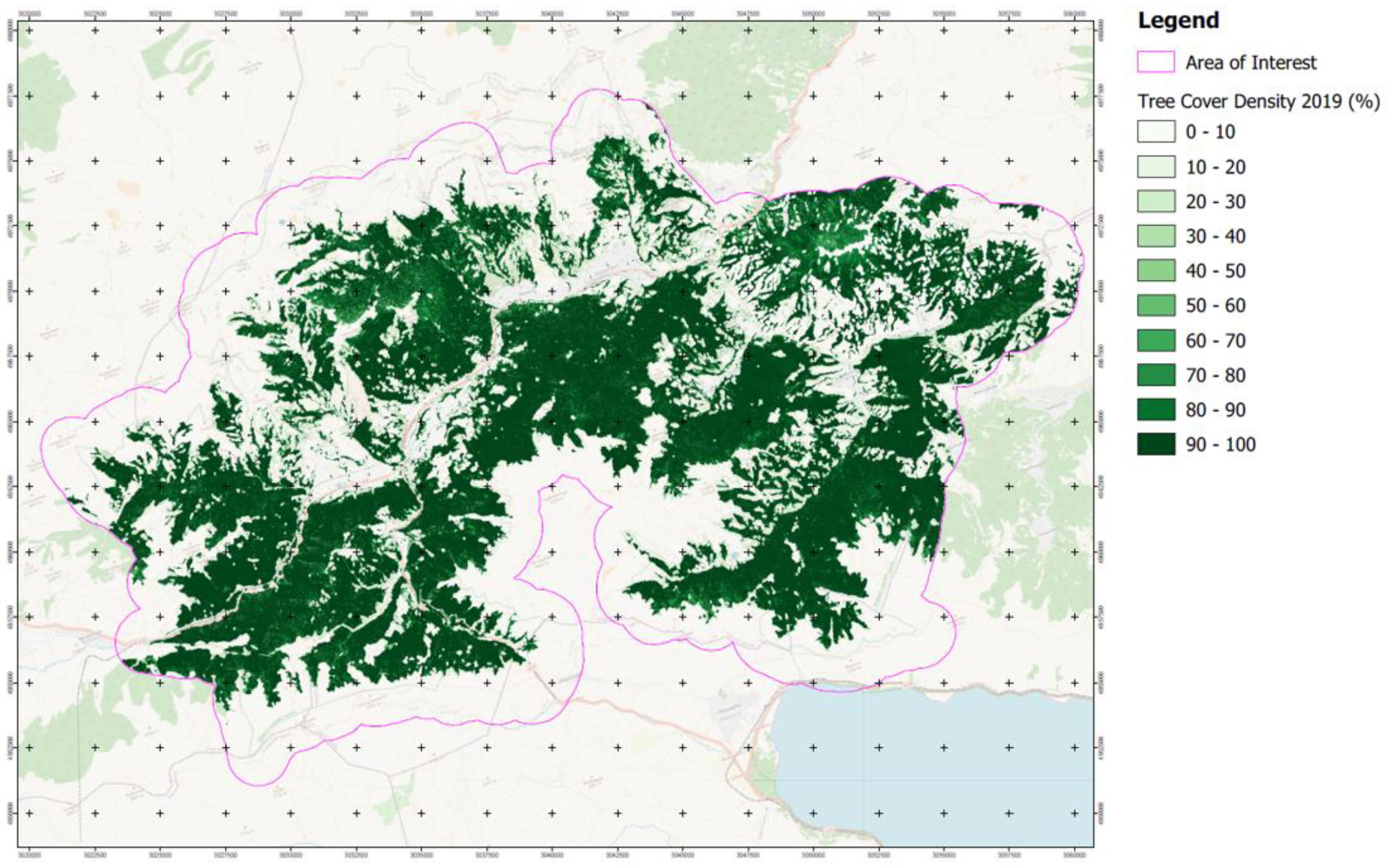
3.1.3. Forest Density Mapping
- (i)
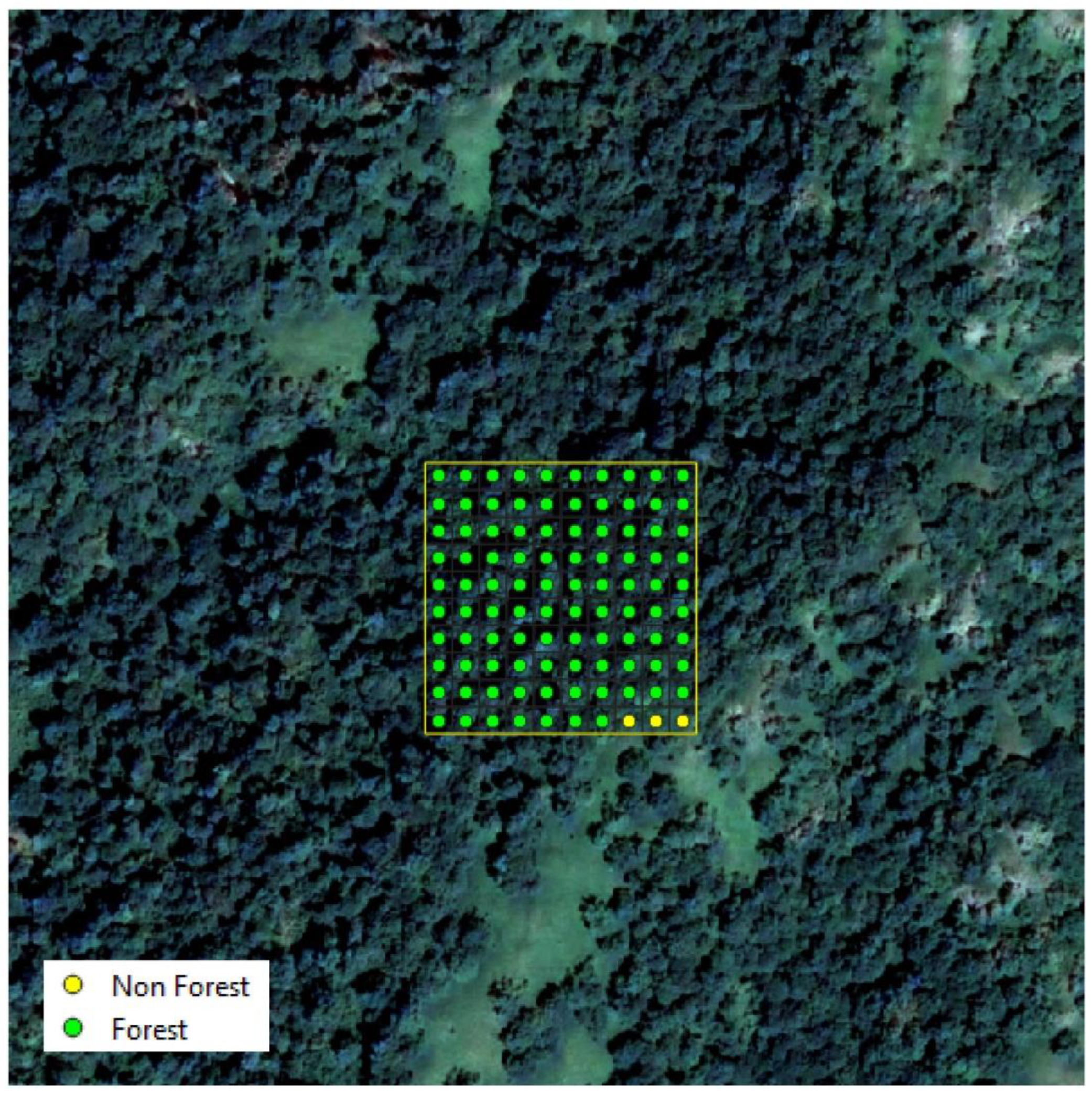
- Sample drawing and interpretation
- (ii)
- Computing vegetation indices
- (iii)
- Multiple linear regression analysis
- (iv)
- Quality Check of the consistency of the Forest Density between all epochs
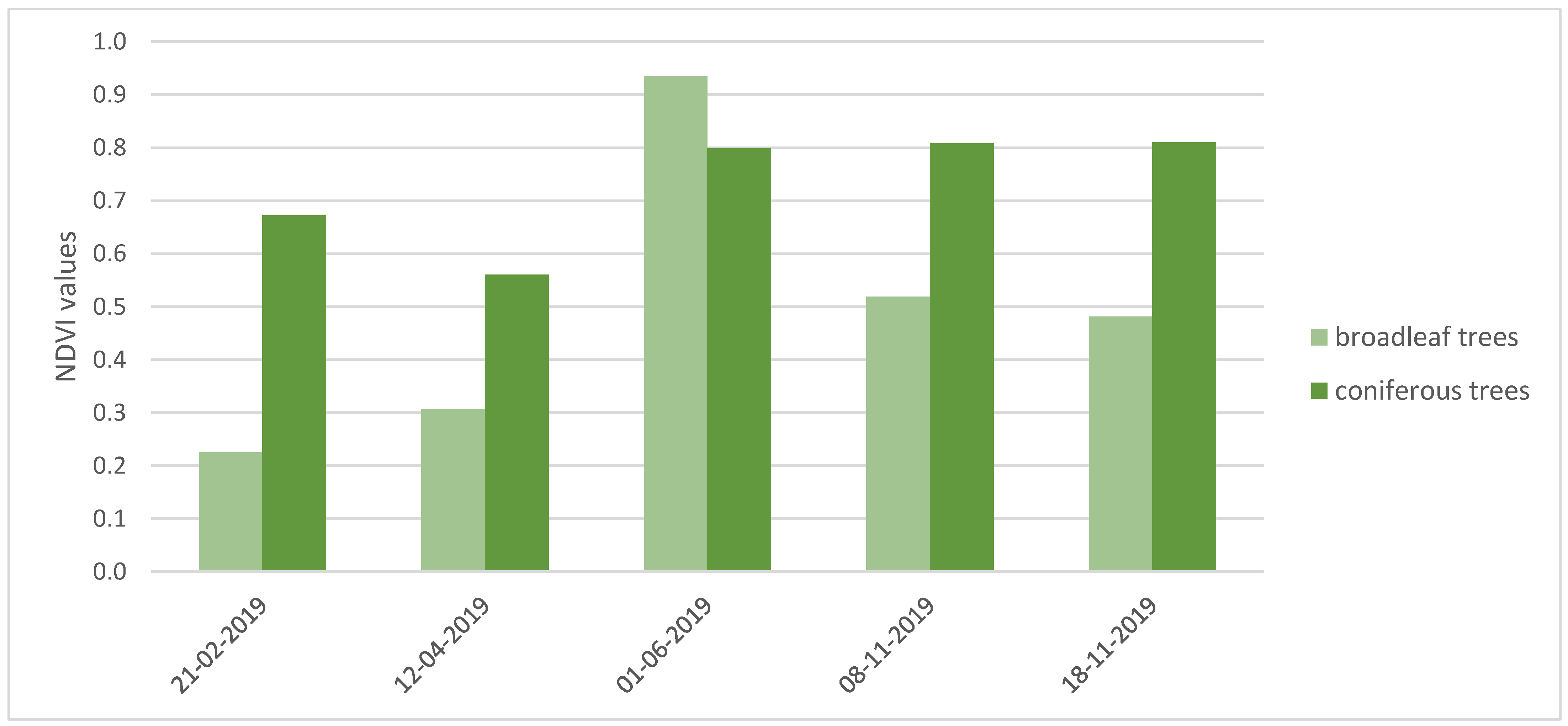
3.1.4. Forest Types
- (i)
- Identification of coniferous reference samples and analysis of their spectral signature over the EO data times-series
- (ii)
- Classification over the whole area
- (iii)
- Crossing with Forest Density to derive Broadleaved and Coniferous Density
- Needle leaved trees
- -
- Pure needle leaved (75%)
- -
- Dominantly needle leaved (50–75%)
- Broadleaved trees
- -
- Pure broadleaved (>75%)
- -
- Dominantly broadleaved (50–75%)
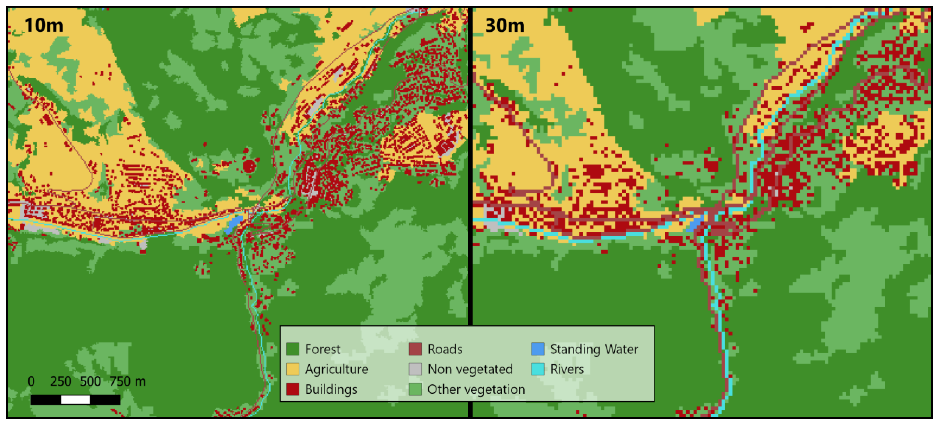
3.2. Land Use and Land Cover Classification and Associated Changes
3.2.1. Specifications
- Forest
- Agriculture (arable land and pastureland)
- Settlements
- Primary roads
- Bare soil
- Other vegetated areas
- Water bodies
- Rivers
3.2.2. Land Use and Land Cover Classification Method
- (i)
- Pre-processing
- (ii)
- Feature Extraction
- (iii)
- Training
- (iv)
- Classification
- (v)
- Post-Processing
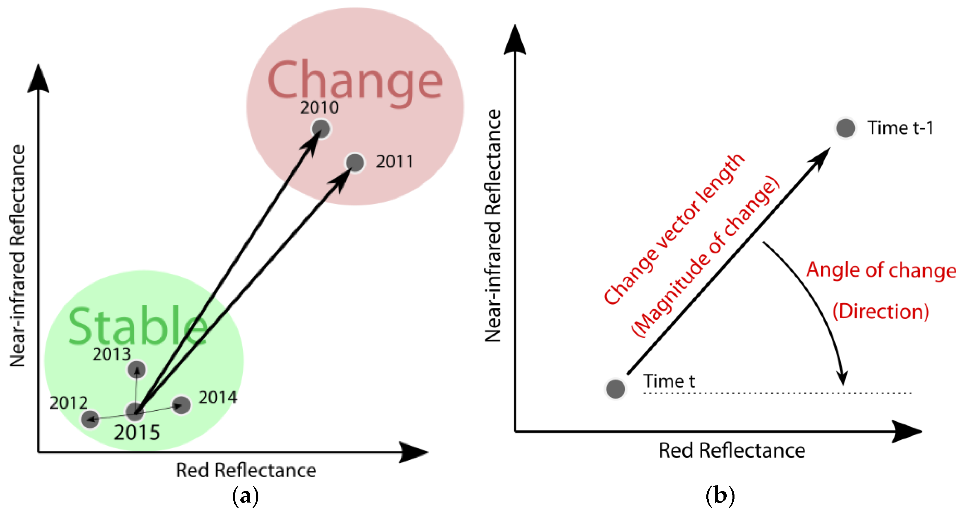
3.2.3. Change Detection
3.2.4. Product Validation
4. Results and Discussion
4.1. Forest Ecosystems Characterization
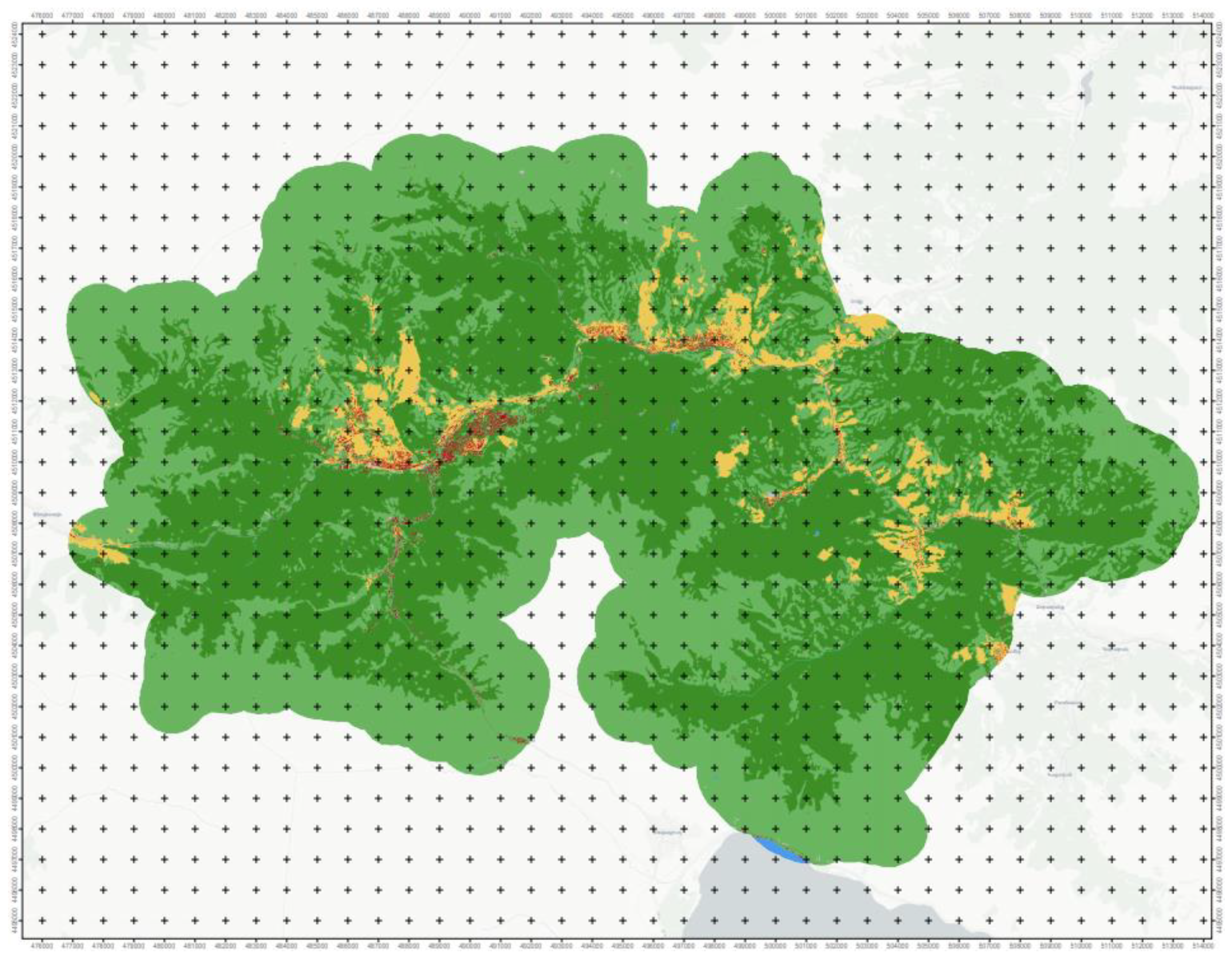
4.1.1. Distribution of Forest Densities and Their Evolution from 1991 to 2019
4.1.2. Characterization of Forest Types
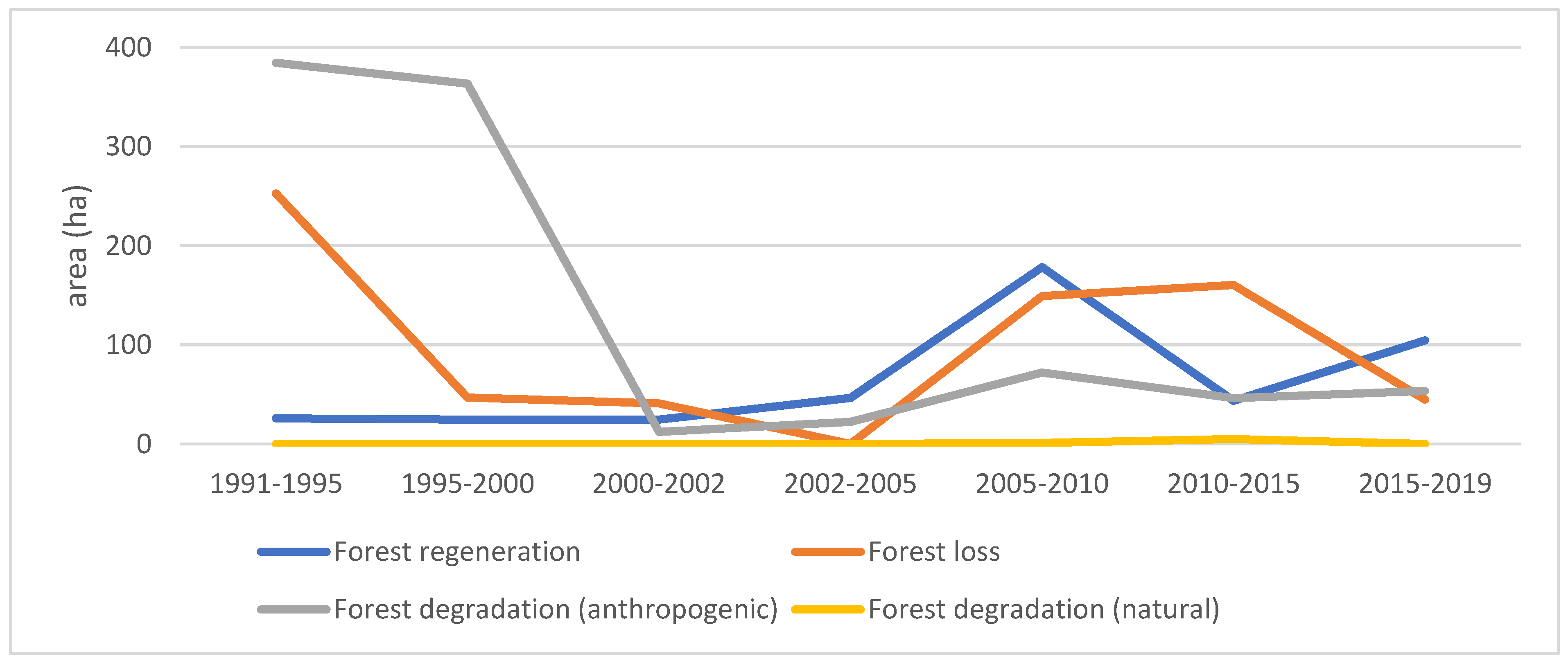
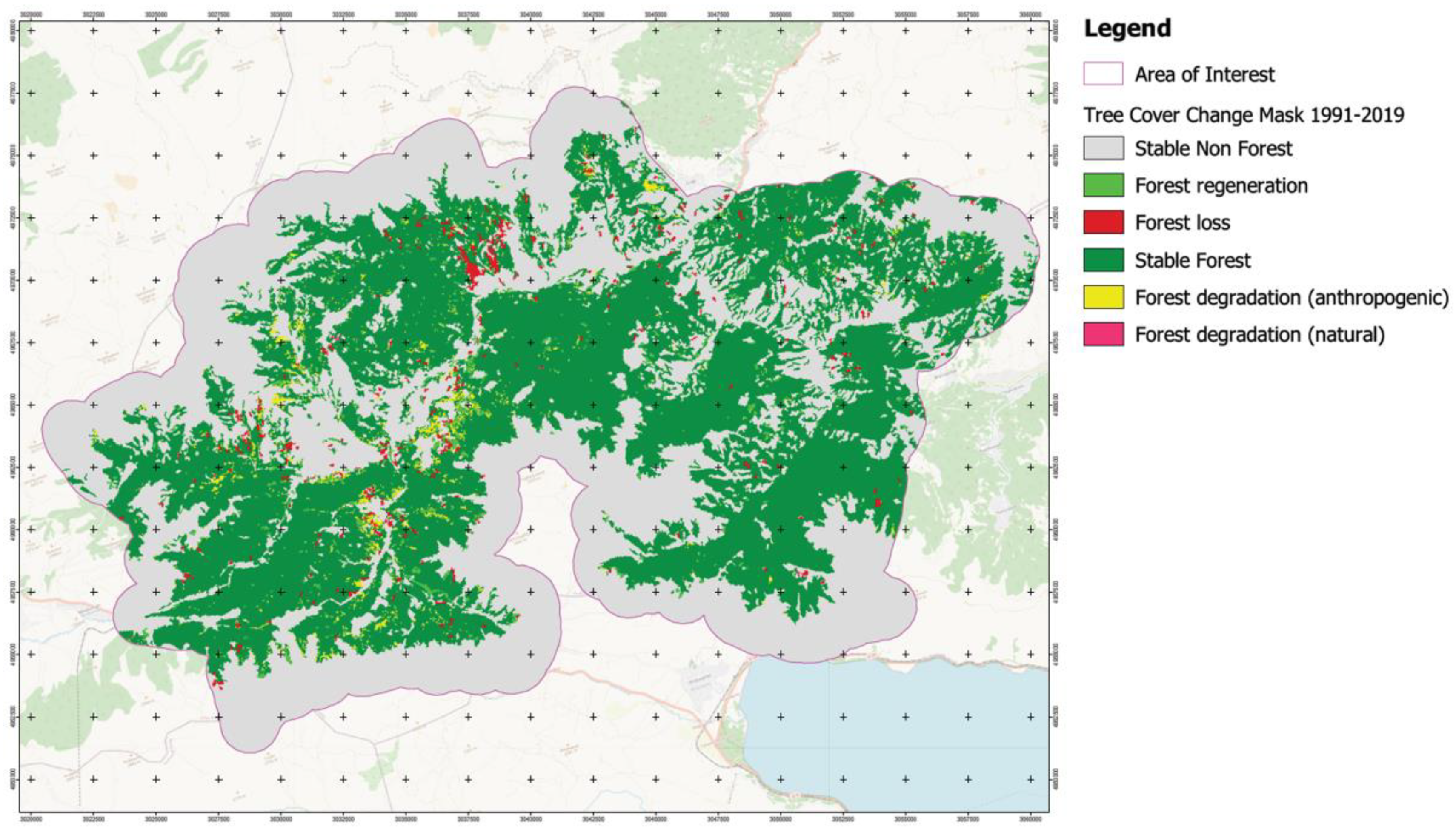
4.1.3. Characterization of Deforestation and Forest Degradation between 1991 and 2019
4.2. Land Use and Land Cover Change
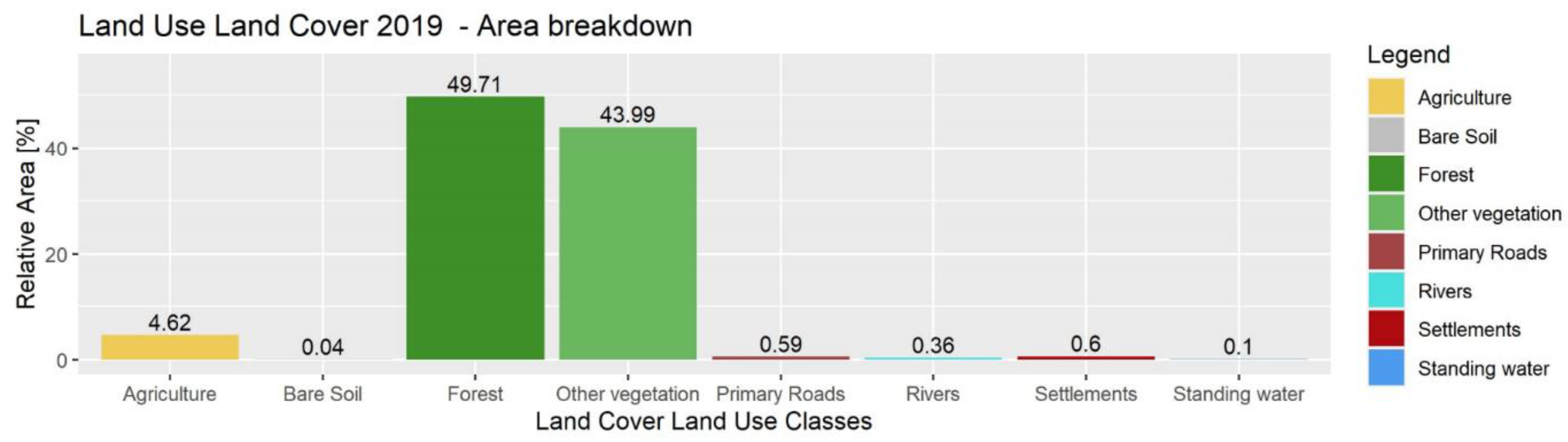
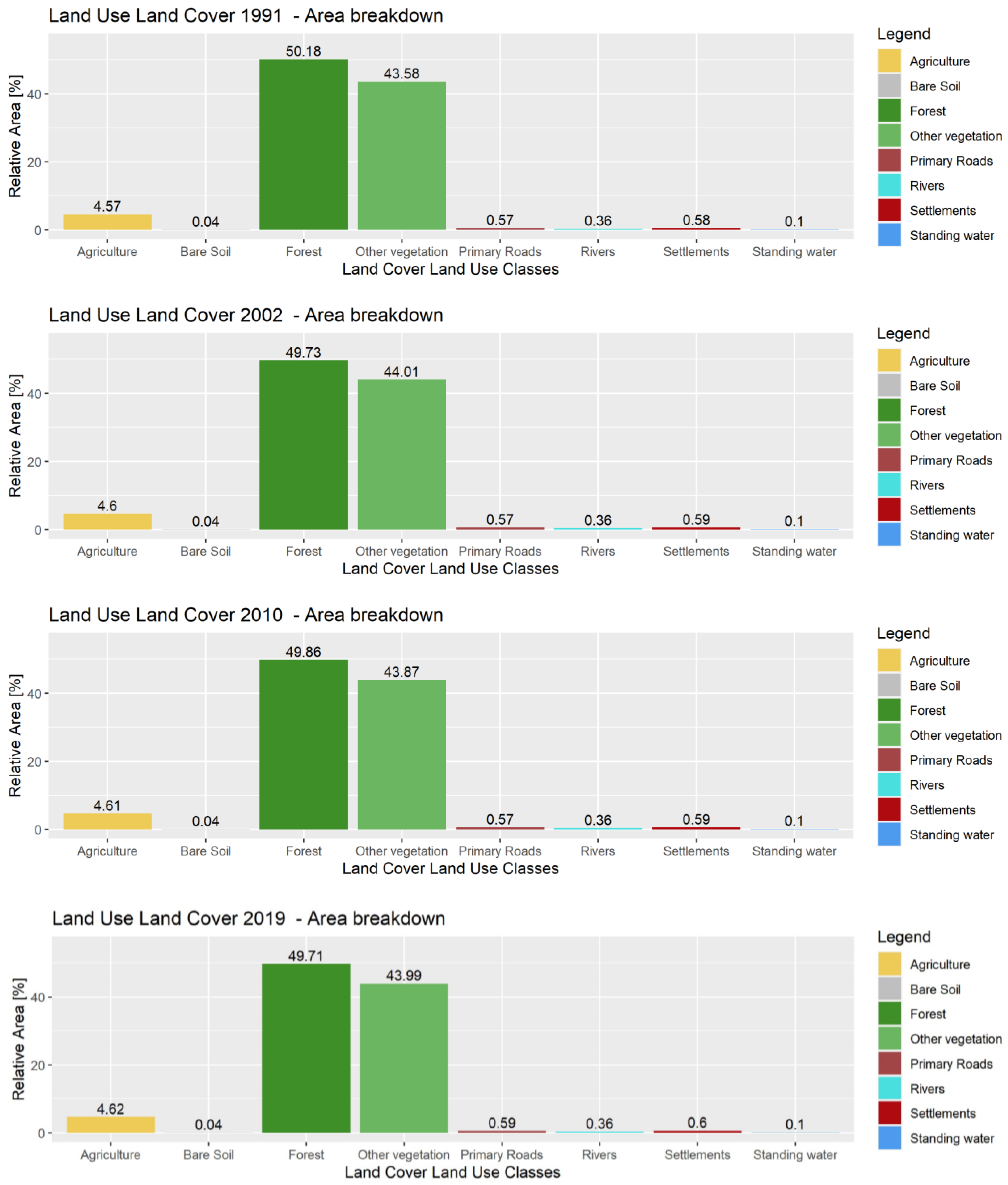
4.2.1. Main Land Use and Land Cover Types
4.2.2. Mapping of Changes from 1991 to 2019
5. Conclusions and Recommendations for Future Work
- Forest densities for each reference years
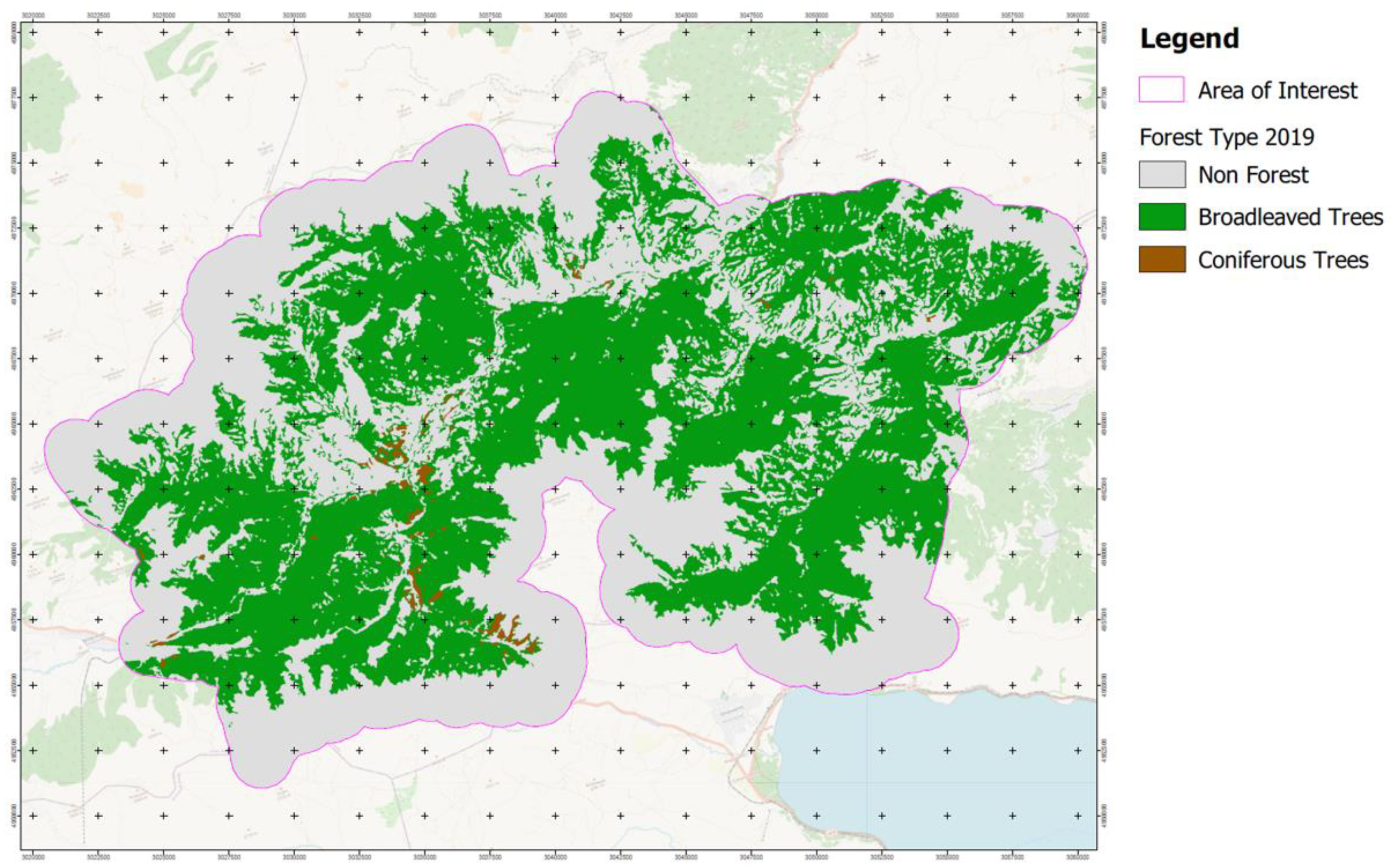
- Forest types for the most recent year (2019)
- Land cover types for each reference year
- In addition, consistent change maps were generated to identify:
- Forest cover changes including the identification of degraded versus deforested areas
- Land cover types of changes
Author Contributions
Funding
Institutional Review Board Statement
Informed Consent Statement
Data Availability Statement
Acknowledgments
Conflicts of Interest
References
- Nationally Designated Protected Areas of the Republic of Armenia. 2019. Available online: https://eni-seis.eionet.europa.eu/east/indicators/d1-nationally-designated-protected-areas-of-the-republic-of-armenia (accessed on 23 July 2021).
- Burns, S.L.; Krott, M.; Sayadyan, H.; Giessen, L. The World Bank Improving Environmental and Natural Resource Policies: Power, Deregulation, and Privatization in (Post-Soviet) Armenia. World Dev. J. 2017, 92, 215–224. [Google Scholar] [CrossRef]
- Nazik, K. Specially Protected Areas of Armenia. Yerevan Tigran Mets. 2004. 54p. Available online: http://www.nature-ic.am/Content/announcements/7337/SPAN_eng.pdf (accessed on 23 July 2021).
- First National Report to the Convention on Biological Diversity, incorporating a Country Study on the Biodiversity of Armenia, Ministry of Nature Protection. 1999. Available online: https://www.cbd.int/doc/world/am/am-nr-01-en.pdf (accessed on 23 July 2021).
- Sixth National Report of the Republic of Armenia, Convention on Biological Diversity. 2019. Available online: https://ace.aua.am/files/2019/05/2019-6th-National-Report-CBD_eng.pdf (accessed on 23 July 2021).
- Ministry of Environment of RA. Available online: http://mnp.am/en/ (accessed on 23 July 2021).
- Hansen, M.C.; Loveland, T.R. A review of large area monitoring of land cover change using Landsat data. Remote Sens. Environ. 2012, 122, 66–74. [Google Scholar] [CrossRef]
- Zhu, Z.; Woodcock, C.E.; Olofsson, P. Continuous monitoring of forest disturbance using all available Landsat imagery. Remote Sens. Environ. 2012, 122, 75–91. [Google Scholar] [CrossRef]
- Inglada, J.; Vincent, A.; Arias, M.; Tardy, B.; Morin, D.; Rodes, I. Operational High Resolution Land Cover Map Production at the Country Scale Using Satellite Image Time Series. Remote Sens. 2017, 9, 35. [Google Scholar] [CrossRef] [Green Version]
- Pelletier, C.; Valero, S.; Inglada, J.; Champion, N.; Dedieu, G. Assessing the robustness of random forests to map land cover with high resolution satellite image time series over large areas. Remote Sens. Environ. 2016, 187, 156–168. [Google Scholar] [CrossRef]
- Sannier, C.; McRoberts, R.E.; Fichet, L.V.; Makaga, E.M.K. Using the regression estimator with Landsat data to estimate proportion forest cover and net proportion deforestation in Gabon. Remote Sens. Environ. 2014, 151, 138–148. [Google Scholar] [CrossRef]
- UNDP in Armenia. Available online: https://www.am.undp.org/content/armenia/en/home/projects/mainstreaming-sustainable-land-and-forest-management-in-mountain.html (accessed on 23 July 2021).
- Merciol, F.; Faucqueur, L.; Damodaran, B.B.; Rémy, P.Y.; Desclée, B.; Dazin, F.; Sannier, C. Geobia at the terapixel scale: Toward efficient mapping of small woody features from heterogeneous vhr scenes. ISPRS Int. J. Geo-Inf. 2019, 8, 46. [Google Scholar] [CrossRef] [Green Version]
- Faucqueur, L.; Morin, N.; Masse, A.; Rémy, P.Y.; Hugé, J.; Kemener, C.; Dazin, F.; Desclée, B.; Sannier, C. A new Copernicus high resolution layer at pan-European scale: The small woody features. Remote Sens. Agric. Ecosyst. Hydrol. 2019, 21. [Google Scholar] [CrossRef]
- Buce Saleh, M.; Nengah Surati, J.; Nitya, A.S.; Dewayany, S.; Ita, C.; Zhang, Y.; Wang, X.; Liu, Q. Algorithm for detecting deforestation and forest degradation using vegetation indices. Telkomnika 2019, 17, 2235–2345. [Google Scholar]
- Pittman, K.; Hansen, M.C.; Becker-Reshef, I.; Potapov, P.V.; Justice, C.O. Estimating Global Cropland Extent with Multi-year MODIS Data. Remote Sens. 2010, 2, 1844–1863. [Google Scholar] [CrossRef] [Green Version]
- Gislason, P.O.; Jon, A.B.; Sveinsson, J.R. Random forests for land cover classification. Pattern Recognit. Lett. 2006, 27, 294–300. [Google Scholar] [CrossRef]
- Olofsson, P. Good practices for estimating area and assessing accuracy of land change. Remote Sens. Environ. 2014, 148, 42–57. [Google Scholar] [CrossRef]
- Congalton, R.G. A review of assessing the accuracy of classifications of remotely sensed data. Remote Sens. Environ. 1991, 37, 35–46. [Google Scholar] [CrossRef]
- Nilsson, S.; Sallnas, O.; Hugosson, M.; Shvidenko, A. The Forest Resources of the Former European USSR; The Parthenon Publishing Group Limited: Carnforth, UK, 1992; 407p. [Google Scholar]
- Sayadyan, H.; Moreno-Sanchez, R. Forest policies, management and conservation in Soviet (1920–1991) and post-Soviet (1991–2005) Armenia. Environ. Conserv. 2006, 33, 1–13. [Google Scholar] [CrossRef]
- Nils, J.; Emily, F. Understanding the Forestry Sector of Armenia: Current Conditions and Choices. Forest Law Enforcement and Governance Program. 2011.


| General | |
| Resolution and Data Input | Forest Density 2019—2 products available:
2010—30 m Landsat 5/7 2005—30 m Landsat 5/7 2002—30 m Landsat 7 2000—30 m Landsat 7 1995—30 m Landsat 5 1991—30 m Landsat 5 Forest Type & Dominant Leaf Type 2019—30 m Landsat 8—Sentinel 2 Forest Degradation/Deforestation Available for each subsequent epoch 1991–1995, 1995–2000, 2000–2002, 2002–2005, 2005–2010, 2010–2015, 2015–2019 as well as for the entire period (1991–2019) at 30 m |
| Geographic Projection | UTM Zone 38N |
| Format | GeoTIFF |
| Data Type | Byte |
| Thematic information | |
| Classes and Coding | Forest Density
|
| Accuracies | |
| Geometric positional accuracy: | 1 pixel |
| Thematic accuracy: | 85% |
| Minimum Mapping Unit (MMU) | |
| Sentinel-2 (10 m) | 0.25 ha (25 px) for forested area (No MMU for other classes and for changes) |
| Landsat 5–8 (30 m) | 1 ha (11 px) for forested area (No MMU for other classes and for changes) |
| Epoch | Satellite Data | Resolution | Comment |
|---|---|---|---|
| 2019 | Sentinel-2 | 10 m | Most recent situation |
| 2015 | Landsat 8 | 30 m | |
| 2010 | Landsat 5 | 30 m | Use of Landsat 5 (due to Landsat 7 SLC error) |
| 2005 | Landsat 5 | 30 m | Use of Landsat 5 (due to Landsat 7 SLC error) |
| 2002 | Landsat 7 | 30 m | Status change from state reserve to national park |
| 2000 | Landsat 7 | 30 m | |
| 1995 | Landsat 5 | 30 m | |
| 1991 | Landsat 5 | 30 m | Armenian Independence |
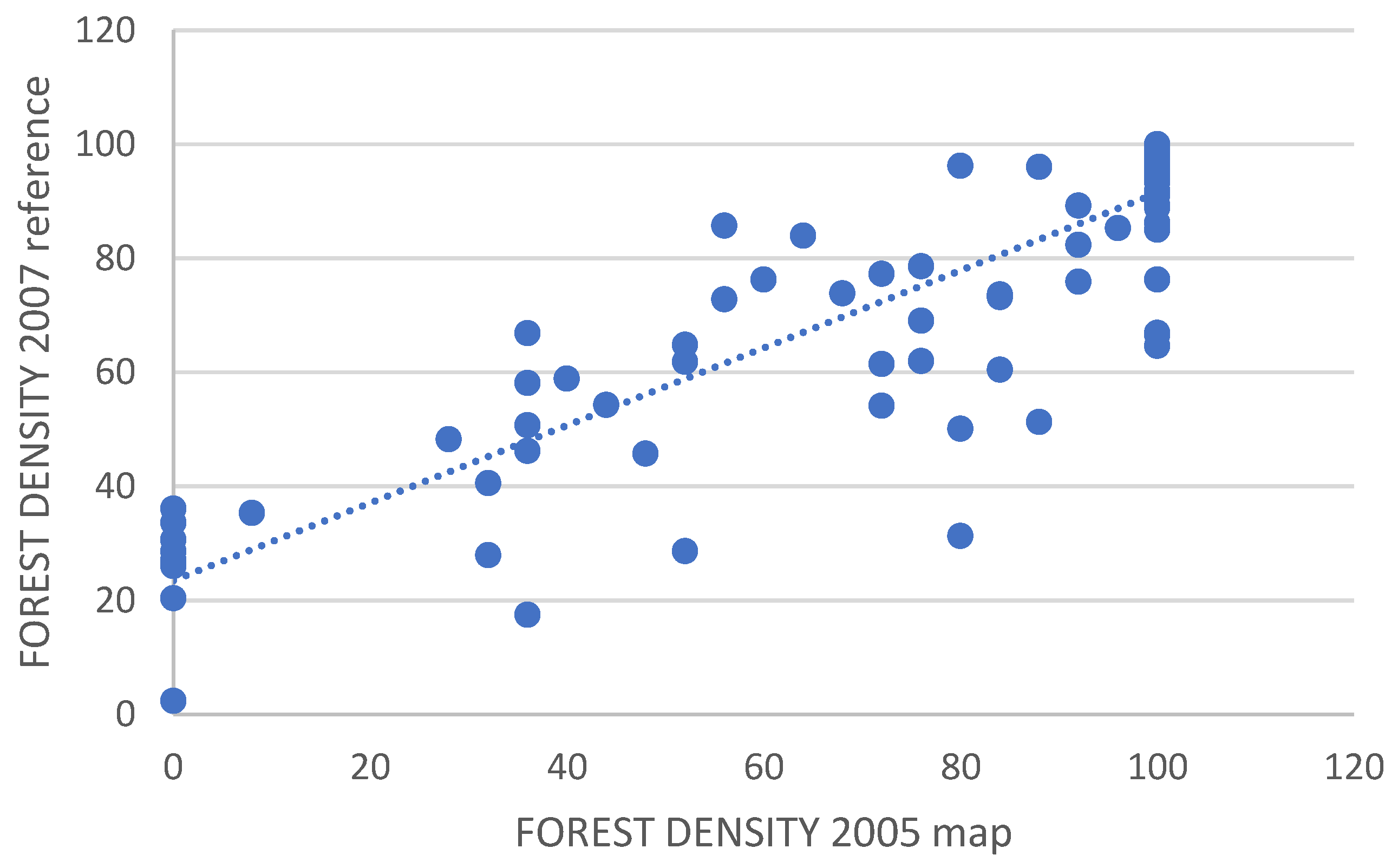
| Epoch | Coeff. Correlation R2 between Reference and Product |
|---|---|
| 1991 | 0.7559 |
| 1995 | 0.6988 |
| 2000 | 0.6991 |
| 2002 | 0.7864 |
| 2005 | 0.7903 |
| 2010 | 0.7988 |
| 2015 | 0.8336 |
| 2019 | 0.8901 |
| 1991–1995 | 1995–2000 | 2000–2002 | 2002–2005 | 2005–2010 | 2010–2015 | 2015–2019 | |
|---|---|---|---|---|---|---|---|
| Forest regeneration (ha) | 26 | 25 | 24 | 47 | 178 | 44 | 104 |
| Forest loss (ha) | 253 | 47 | 41 | 0 | 149 | 160 | 45 |
| Forest degradation (anthropogenic) (ha) | 384 | 363 | 12 | 22 | 72 | 46 | 53 |
| Forest degradation (natural) (ha) | 0 | 0 | 0 | 0 | 1 | 5 | 0 |
| Ground Truth | |||||||||||
|---|---|---|---|---|---|---|---|---|---|---|---|
| Forest | Agriculture | Settlement | Primary Roads | Bare Soil | Other Vegetation | Standing Water | Rivers | # Samples | User Accuracy | ||
| Classification | Forest | 26 | 0 | 0 | 0 | 0 | 4 | 0 | 0 | 30 | 86.67% |
| Agriculture | 1 | 22 | 0 | 0 | 0 | 7 | 0 | 0 | 30 | 73.33% | |
| Settlement | 0 | 1 | 23 | 1 | 2 | 3 | 0 | 0 | 30 | 76.67% | |
| Primary roads | 2 | 0 | 0 | 28 | 0 | 0 | 0 | 0 | 30 | 93.33% | |
| Bare soil | 0 | 0 | 0 | 2 | 23 | 5 | 0 | 0 | 30 | 76.67% | |
| Other vegetation | 1 | 1 | 0 | 0 | 0 | 28 | 0 | 0 | 30 | 93.33% | |
| Standing water | 1 | 0 | 0 | 0 | 0 | 0 | 29 | 0 | 30 | 96.67% | |
| Rivers | 1 | 0 | 0 | 0 | 1 | 1 | 0 | 27 | 30 | 90.00% | |
| Totals | 32 | 24 | 23 | 31 | 26 | 48 | 29 | 27 | 240 | ||
| Producer accuracy | 81.25% | 91.67% | 100.00% | 90.32% | 88.46% | 58.33% | 100.00% | 100.00% | |||
| Overall accuracy | 85.83% | ||||||||||
| Ground Truth | ||||||||||||
|---|---|---|---|---|---|---|---|---|---|---|---|---|
| Forest | Agriculture | Settlement | Primary Roads | Bare Soil | Other Vegetation | Standing Water | Rivers | # Samples | User Accuracy | |||
| Classification | Forest | 26 | 0 | 0 | 0 | 0 | 4 | 0 | 0 | 30 | 86.67% | |
| Agriculture | 0 | 24 | 0 | 0 | 0 | 6 | 0 | 0 | 30 | 80.00% | ||
| Settlement | 0 | 0 | 28 | 1 | 0 | 1 | 0 | 0 | 30 | 93.33% | ||
| Primary roads | 2 | 0 | 0 | 26 | 0 | 0 | 0 | 0 | 28 | 92.86% | ||
| Bare soil | 0 | 0 | 0 | 5 | 22 | 3 | 0 | 0 | 30 | 73.33% | ||
| Other vegetation | 3 | 1 | 0 | 0 | 0 | 26 | 0 | 0 | 30 | 86.97% | ||
| Standing water | 1 | 0 | 0 | 0 | 0 | 0 | 28 | 1 | 30 | 93.33% | ||
| Rivers | 1 | 0 | 0 | 0 | 0 | 1 | 0 | 28 | 30 | 93.33% | ||
| Totals | 33 | 25 | 28 | 32 | 22 | 41 | 28 | 29 | 238 | |||
| Producer accuracy | 78.79% | 96.00% | 100.00% | 81.25% | 100.00% | 63.41% | 100.00% | 96.55% | ||||
| Overall accuracy | 87.39% | |||||||||||
| Ground Truth | ||||||||||||
|---|---|---|---|---|---|---|---|---|---|---|---|---|
| Forest | Agriculture | Settlement | Primary Roads | Bare Soil | Other Vegetation | Standing Water | Rivers | # Samples | User Accuracy | |||
| Classification | Forest | 29 | 0 | 0 | 0 | 0 | 1 | 0 | 0 | 30 | 96.67% | |
| Agriculture | 1 | 22 | 0 | 0 | 0 | 7 | 0 | 0 | 30 | 73.33% | ||
| Settlement | 1 | 0 | 26 | 1 | 1 | 1 | 0 | 0 | 30 | 86.67% | ||
| Primary roads | 1 | 0 | 0 | 29 | 0 | 0 | 0 | 0 | 30 | 96.67% | ||
| Bare soil | 1 | 0 | 0 | 2 | 23 | 4 | 0 | 0 | 30 | 76.67% | ||
| Other vegetation | 1 | 0 | 0 | 0 | 0 | 29 | 0 | 0 | 30 | 96.67% | ||
| Standing water | 0 | 0 | 0 | 0 | 0 | 2 | 28 | 0 | 30 | 93.33% | ||
| Rivers | 0 | 0 | 0 | 0 | 0 | 2 | 0 | 28 | 30 | 93.33% | ||
| Totals | 34 | 22 | 26 | 32 | 24 | 46 | 28 | 28 | 240 | |||
| Producer accuracy | 85.29% | 100.00% | 100.00% | 90.63% | 95.83% | 63.04% | 100.00% | 100.00% | ||||
| Overall accuracy | 89.17% | |||||||||||
Publisher’s Note: MDPI stays neutral with regard to jurisdictional claims in published maps and institutional affiliations. |
© 2021 by the authors. Licensee MDPI, Basel, Switzerland. This article is an open access article distributed under the terms and conditions of the Creative Commons Attribution (CC BY) license (https://creativecommons.org/licenses/by/4.0/).
Share and Cite
Morin, N.; Masse, A.; Sannier, C.; Siklar, M.; Kiesslich, N.; Sayadyan, H.; Faucqueur, L.; Seewald, M. Development and Application of Earth Observation Based Machine Learning Methods for Characterizing Forest and Land Cover Change in Dilijan National Park of Armenia between 1991 and 2019. Remote Sens. 2021, 13, 2942. https://doi.org/10.3390/rs13152942
Morin N, Masse A, Sannier C, Siklar M, Kiesslich N, Sayadyan H, Faucqueur L, Seewald M. Development and Application of Earth Observation Based Machine Learning Methods for Characterizing Forest and Land Cover Change in Dilijan National Park of Armenia between 1991 and 2019. Remote Sensing. 2021; 13(15):2942. https://doi.org/10.3390/rs13152942
Chicago/Turabian StyleMorin, Nathalie, Antoine Masse, Christophe Sannier, Martin Siklar, Norman Kiesslich, Hovik Sayadyan, Loïc Faucqueur, and Michaela Seewald. 2021. "Development and Application of Earth Observation Based Machine Learning Methods for Characterizing Forest and Land Cover Change in Dilijan National Park of Armenia between 1991 and 2019" Remote Sensing 13, no. 15: 2942. https://doi.org/10.3390/rs13152942
APA StyleMorin, N., Masse, A., Sannier, C., Siklar, M., Kiesslich, N., Sayadyan, H., Faucqueur, L., & Seewald, M. (2021). Development and Application of Earth Observation Based Machine Learning Methods for Characterizing Forest and Land Cover Change in Dilijan National Park of Armenia between 1991 and 2019. Remote Sensing, 13(15), 2942. https://doi.org/10.3390/rs13152942