1. Introduction
The implementation of hydrological models has become common practice in the prediction of river discharge flow and volume at basin scale. These models can be employed in analyses of land use and climate change scenarios [
1], flood prediction [
2], and rainfall-runoff processes [
3]. For these types of analysis, one of the most important variables is precipitation. Based on precipitation data availability, it is important to select a proper hydrological model to take advantage of precipitation accuracy.
Distributed and semi-distributed hydrological models are the most popular model types. These models require aerial precipitation datasets, meaning that the spatial variability within the basin is important. In this regard, an alternative option is the use of rain gauges as precipitation input data [
4]. Prior to the usage of rain gauge data, data pre-processing (i.e., gridding) is required to change its spatial distribution from isolated points to a distributed grid. Many previous studies have attempted to determine the optimal interpolation method to use with point rain gauges [
5,
6,
7]; unfortunately, the rain gauges can be affected by atmospheric effects [
8] and the possibility of instrument failure, among other issues. When applying interpolation methods, the number and location of rain gauges in some basins are often insufficient and, in some instances, may be extremely poor. According to the World Meteorological Organization (WMO), the installation density of rain gauges is determined by the type of surface topography [
9]. For example, the density in Mexico is 804 km
2 per station, which is an acceptable value according to the WMO. In the case of Bolivia, however, the density is much sparser at about 2922 km
2 per station. For this reason, an alternative approach employed in hydrological models is the use of satellite-based products to obtain precipitation data.
Satellite-based precipitation (SBP) data is obtained by using different sensors onboard satellites. These sensors can scan or retrieve water molecules in different phases, such as vapor. Algorithms are then used on the retrieved signals to generate gridded precipitation information at different spatial and temporal resolutions. Popular SBP products include Global Satellite Mapping of Precipitation (GSMaP) [
10,
11,
12] and Climate Hazards Group Infrared Precipitations with Stations (CHIRPS) [
13,
14].
Previous studies comparing the accuracy of these products to rain gauges and radar have shown acceptable results in favor of SBP [
15]. Despite the advantages of using these measurements, SBP products have difficulty in generating precipitation data due to the geographic and geomorphological conditions in some regions of the planet [
16]. For example, the Integrated Multi-satellite Retrievals for GPM (IMERG) product presents acceptable results in arid regions, however, this product requires calibration to improve rainfall data [
17]. Due to the need to improve precipitation data, new generations of satellite-based products with better accuracy are required. These new versions have been evaluated to verify the improvement in data quality in relation to previous versions. For example, a study of the Global Precipitation Measurement (GPM) mission’s new generation was presented in Malaysia [
18], an analysis of two versions of the Tropical Rainfall Measuring Mission (TRMM) v7 was conducted in China [
19], and the evolution of TRMM to IMERG [
20].
An alternative to employing distributed precipitation data is the generation of new products that combine rain gauges and SBP. For example, using several satellite-based products with inverse distance weighting (IDW) interpolation generated a new gridded product for Java Island, Indonesia [
21]. However, a robust approach is needed to validate these new improved products.
The objective of this study was to evaluate satellite-based precipitation products and generate combined products for different hydrological applications. The SBP products selected were GSMaP and CHIRPS. To generate combined products, an iterative method was proposed at the sub-basin scale using local rain gauges. The obtained products were then evaluated, randomly reducing 10% of available gauges. Finally, an estimation of river discharge flow at three major basins in Bolivia was carried out.
2. Materials and Methods
2.1. Study Area
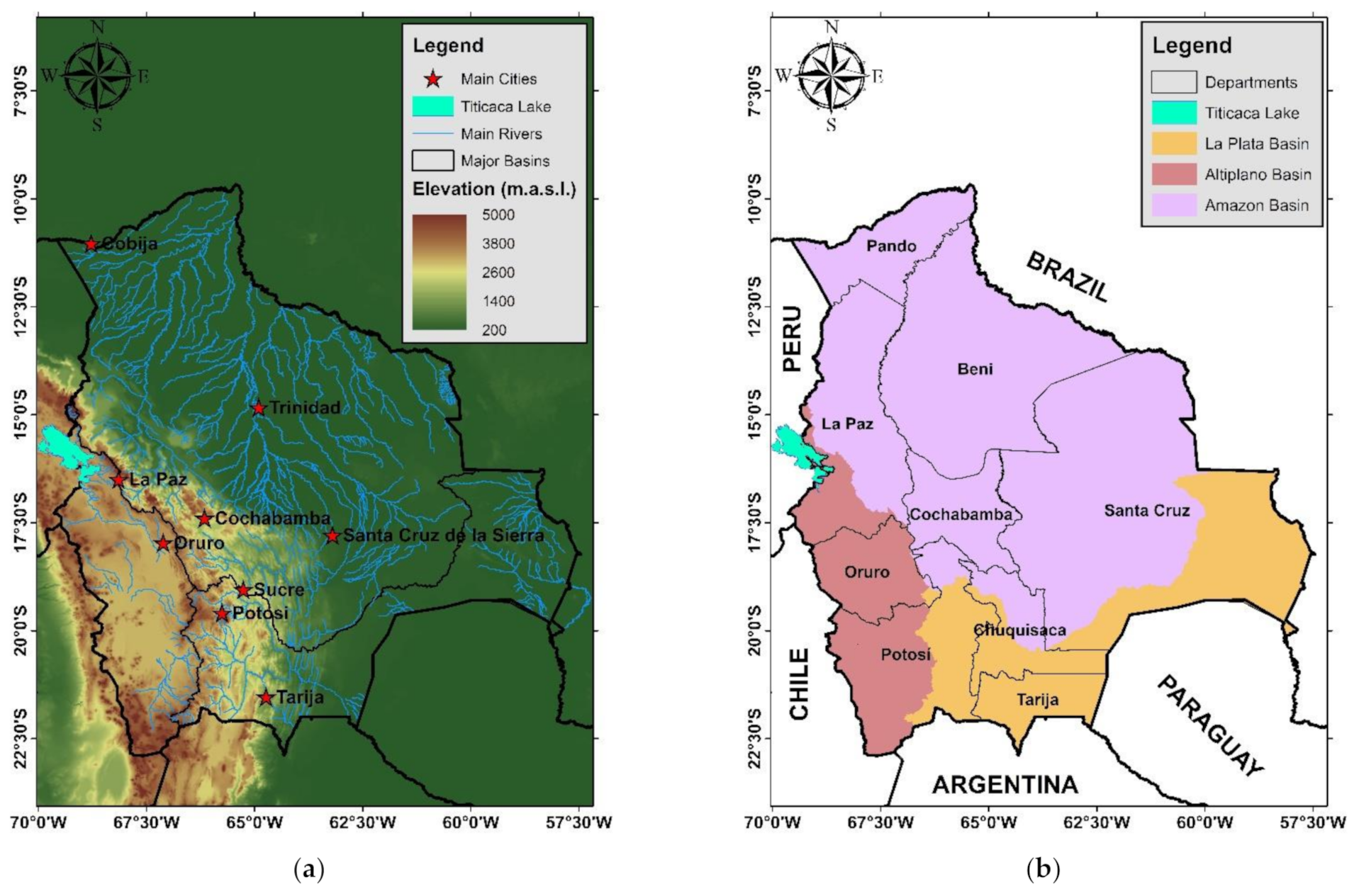
The country of Bolivia has an onshore area of 1,098,006 km
2, with elevation values principally in the range of 200 to 5000 m above sea level (m.a.s.l.). This can be divided into three ecological regions: highlands (west and southwest of the country), valleys (middle region of the country), and lowlands (north and east of the country); these can be seen in
Figure 1a.
Hydrographically, the country is formed by three major basins: the Altiplano, Amazon, and La Plata (
Figure 1b). The Altiplano basin covers the southwest of La Paz and Oruro, and the eastern part of the Potosi department. The Amazon basin comprises Pando, Beni, Cochabamba, the northeast of La Paz, north of Potosi and Chuquisaca, and the northwestern part of the Santa Cruz department. The La Plata basin comprises Tarija, the eastern part of Potosi, the south of Chuquisaca, and the southeast of the Santa Cruz departments.
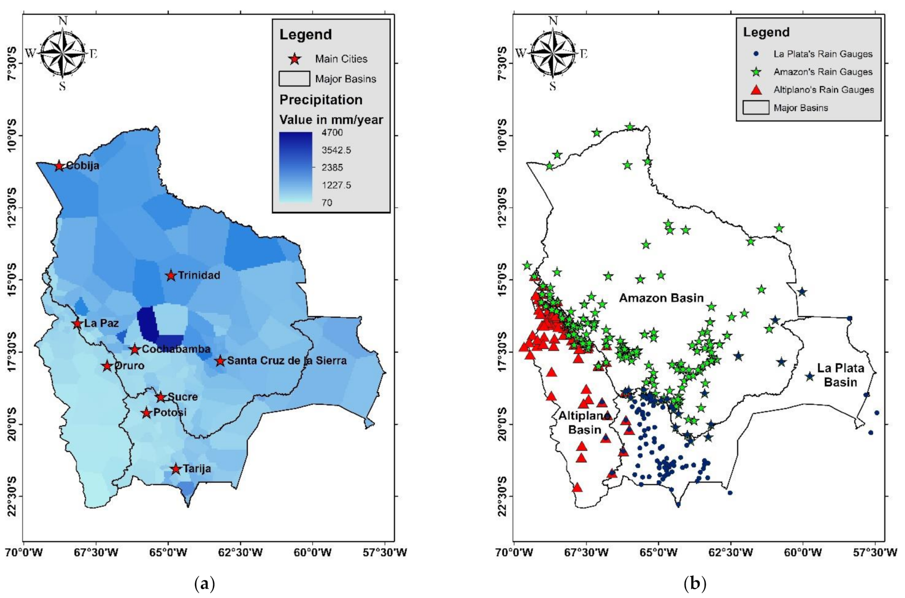
The Altiplano basin covers an area of 151,722 km
2, making it the smallest major basin in the country. This basin is endorheic and contains an ecological region of highlands in almost all areas. The basin has precipitation of around 70 to 750 mm per year (
Figure 2a) with an average runoff of 79% [
22]. In this study, 84 rain gauges from the Altiplano basin were used (
Figure 2b).
The Amazon basin covers 720,792 km
2, the largest basin out of the three mentioned in this study. The basin presents three ecological regions: highlands in the southeast of the basin, valleys in the middle region of Cochabamba and Chuquisaca departments, and lowlands in the northeast of the basin. The Amazon basin discharges into the Atlantic Ocean, and the precipitation in this basin represents the highest values in the country. The mean precipitation in much of the basin is around 500 to 3000 mm/year and the region with the highest precipitation has around 3000 to 4700 mm/year (
Figure 2a) with an average runoff of 65% [
22]. In this study, 179 nine rain gauges were used in this area (
Figure 2b).
The La Plata basin covers 225,492 km
2. Like the Amazon basin, the La Plata basin discharges into the Atlantic Ocean and has three ecological regions: highlands in the west zone, valleys in the middle of the Chuquisaca and Tarija departments, and lowlands in the east zone of the basin. The mean precipitation is around 400 to 2500 mm/year (
Figure 2a) with an average runoff around 73% to 78% [
22]. In this study, 112 rain gauges were used from the La Plata Basin (
Figure 2b).
2.2. Data Set
CHIRPS is an SBP product that was developed at the Climate Hazards Center at the University of California, Santa Barbara, to support a global early warning system for drought [
14]. This product has a spatial resolution of 0.05° (approximately 5 km) and three different temporal resolutions (daily, fortnightly, and monthly). CHIRPS implements three phases to generate the dataset: namely the Climate Hazards Group Precipitation Climatology (CHPclim), CHIRP and CHIRPS. In the case of the first, an algorithm uses the satellite means, normal stations, and geographic conditions (i.e., elevation, latitude, and longitude) to generate CHPclim. This data is a necessary aspect for calculating the precipitation percentage; this percentage is obtained by dividing the cold cloud duration (CCD) precipitation estimates and the mean CCD precipitation estimates (the CCD employs an infrared sensor). By combining the CHPclim and precipitation percentage data, the CHIRP dataset is obtained. To integrate data from the gauge stations to generate CHIRPS, data from many public and private institutions are used. With this information, the Climate Hazards Group generates an IDW interpolation map and calculates the percentage bias compared to CHIRP. Subsequently, using another algorithm, the generation of CHIRPS is complete [
13]. CHIRPS employs around 40 rain gauges in Bolivia to perform ground validation.
The Global Satellite Mapping of Precipitation (GSMaP) is an SBP product that was developed by the Japan Aerospace Exploration Agency (JAXA). The current version of this precipitation product has a spatial resolution of 0.1° (approximately 10 km) and a temporal resolution of an hour. The calculation method of this product includes precipitation data from the TRMM Microwave Imager, data from the Advanced Microwave Scanning Radiometer for the Earth Observation System (AMSR-E) of NASA, data from the AMSR of JAXA, and information from three special sensor microwave/imagers (SSM/I) [
10,
11]. By integrating constraints from moving vector by Kalman-filter (MVK) data, GSMaP map products were generated with the aforementioned spatial and temporal resolutions [
12] and distributed as GSMaP_MVK version 6.
On evaluation, GSMaP MVK presented difficulties in measuring the level of real precipitation that arrived on the surface. For this reason, adjustments to this product were needed to include more surface information and gauge stations. With an adjustment method using the NOAA Climate Prediction Center (CPC) global rain gauge data set [
23], the GSMaP_Gauge version 6 has been available since 2014. This version of GSMAP uses about 32 rain gauges in Bolivia to perform ground validation.
The rain gauge-adjustment algorithm of the GSMaP_Gauge product was modified in 2019, and after this modification, the alternative GSMaP_GREV precipitation product became available. Both the GSMaP_Gauge and the GSMaP_GREV datasets are available with three days of data latency [
11].
2.3. Development Method
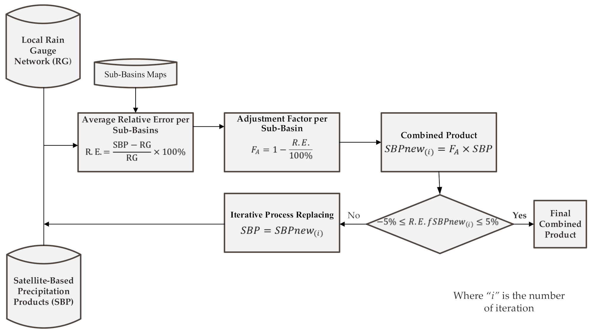
The method of generation is based on the approach that was previously used in the Katari, Pilcomayo, and Rio Grande basins [
24]. It was therefore necessary to pre-process the rain gauge precipitation data and SBP products to be able to combine the data sets.
In the case of the rain gauges, it was necessary to use ordinary kriging interpolation to produce gridded data. Using the rain gauges employed in the “Balance Hídrico Superficial de Bolivia” (BHSB) [
22], the precipitation maps for Bolivia were generated.
The SBP products require that the spatial and temporal resolution values should be the same between different datasets. The SBP products used in this study had a maximum spatial resolution of 0.05°; some datasets had coarser resolution. For this study, a resolution of 0.05° was selected for the data processing. In terms of temporal resolution, the generation approach requires this to be monthly.
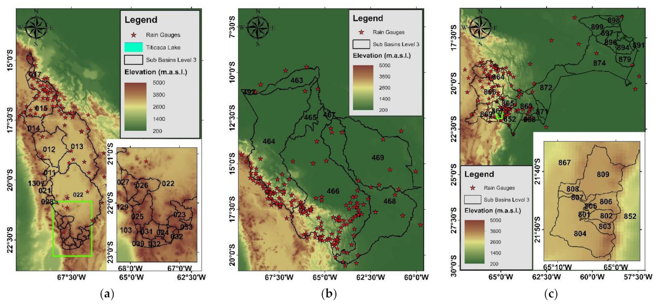
This method performs iteration at a sub-basin scale. For this reason, the official subdivision of basins in Bolivia was used, which is based on the Pfafstetter coding system, as shown in
Figure 3. In this study, we use the third level of this classification scheme.
After preparation of the rain gauge and SBP datasets at monthly temporal resolution, the relative error was calculated, and the mean relative error was obtained for the sub-basins of the three main study basins. With this, the adjustment factor was calculated using the following equation:
where
FA is the adjustment factor and
R.E. is the relative error.
With the adjustment factor calculated per sub-basin and the pre-processed SBP data, the combined products were generated. The combined products then needed to be validated with a new average relative error per sub-basin. For this study, a relative error of ±5% was considered acceptable in all sub-basins. Where this condition was not met, the process continued with further iteration steps. In the case of the three basins in this study, the final combined product was the fifth iteration.
Figure 4 shows a flow chart with a resume of this process.
2.4. Validation Approach
This method combines satellite-based precipitation products with the national rain gauge network through a series of iterations. To analyze the generation method, 10 scenarios were randomly selected that use 90% of the rain gauges in the country. With these 10 new rain gauge data sets, 10 new kriging precipitation maps were generated. In total, 20 combined products were generated: 10 products combined 90% of rain gauges and CHIRPS products, and 10 products combined 90% of rain gauges with GSMaP products.
Afterward, these 20 new combined products were analyzed.
Figure 5 shows a selection of rain gauges used to generate the kriging precipitation map.
In this study, the sub-basins were considered to be the units of analysis; these were chosen because the priority was to generate a product that could be employed in hydrological models. The statistical indicators selected for data evaluation purposes were the determination coefficient (R
2), the correlation coefficient (R), the average ratio (%), the average bias (mm), the mean absolute error (MAE), the root mean square error (RMSE), and the Nash and Sutcliffe efficiency (NSE). These indicators were selected because this proves the validity of the approach; moreover, they have been previously calculated in other studies of sub-basins in Bolivia [
25].
2.5. Applicability of Combined Products in Distributed Hydrological Modeling
Combined precipitation products can be used for different types of application. For example, the combined precipitation dataset can be useful for calculating water budgets using hydrological models based on sub-basin or hydrological units’ analysis.
In this study, an exercise was carried out to show the usage of combined precipitation products. Initially, it is possible to estimate the river discharge flow (
Q) for each sub-basin using the reported runoff coefficients (
c), the extent of precipitation (
P), and the basin surface area (
A). In this case, the selected equation was:
As a result, the generated discharge flow for the three study basins was obtained and compared with values from the BHSB datasets of 2012 [
26] and 2018 [
22]. The BHSB monthly mean precipitation was used for comparison with the SBP products and the combined products.
Equation (2) is a simple way to obtain river discharge. In the case of the BHSB datasets, the Temez model was used for calculation of the 2012 version [
26] and the WEAP model for the 2018 version [
22]. The objective of the comparison between datasets is to show the potential of the combined products generated in this study.
3. Results
3.1. Global Satellite Mapping of Precipitation (GSMaP) Product Analysis
For this study, JAXA provided access to their database of precipitation products. The version with the most precipitation information (i.e., 6th version) was selected; this version of GSMaP presents three products with different characteristics for the period 2000–2016.
GSMaP_MVK (
Figure 6a) shows significant value overestimates in the southern part of the Amazon basin and the northeastern part of La Plata Basin. With precipitation in excess of 3500 mm/year, this product presents more zones with high precipitation. GSMaP_Gauge (
Figure 6b) also shows an overestimate in the northern part of the Amazon Basin; another characteristic of this product is a regular distribution of precipitation in the study basins. By contrast, GSMaP_GREV (
Figure 6c) shows only a small area with high precipitation values in the eastern part of the Amazon basin. This product does not present the high precipitation values seen in areas of the other GSMaP products.
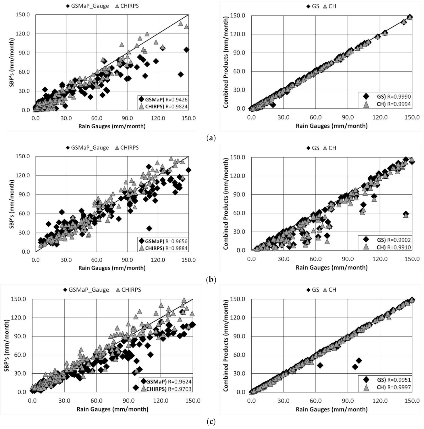
To understand the differences between the GSMaP products, we used statistical indicators in combination with scatter plots in relation to rain gauge data.
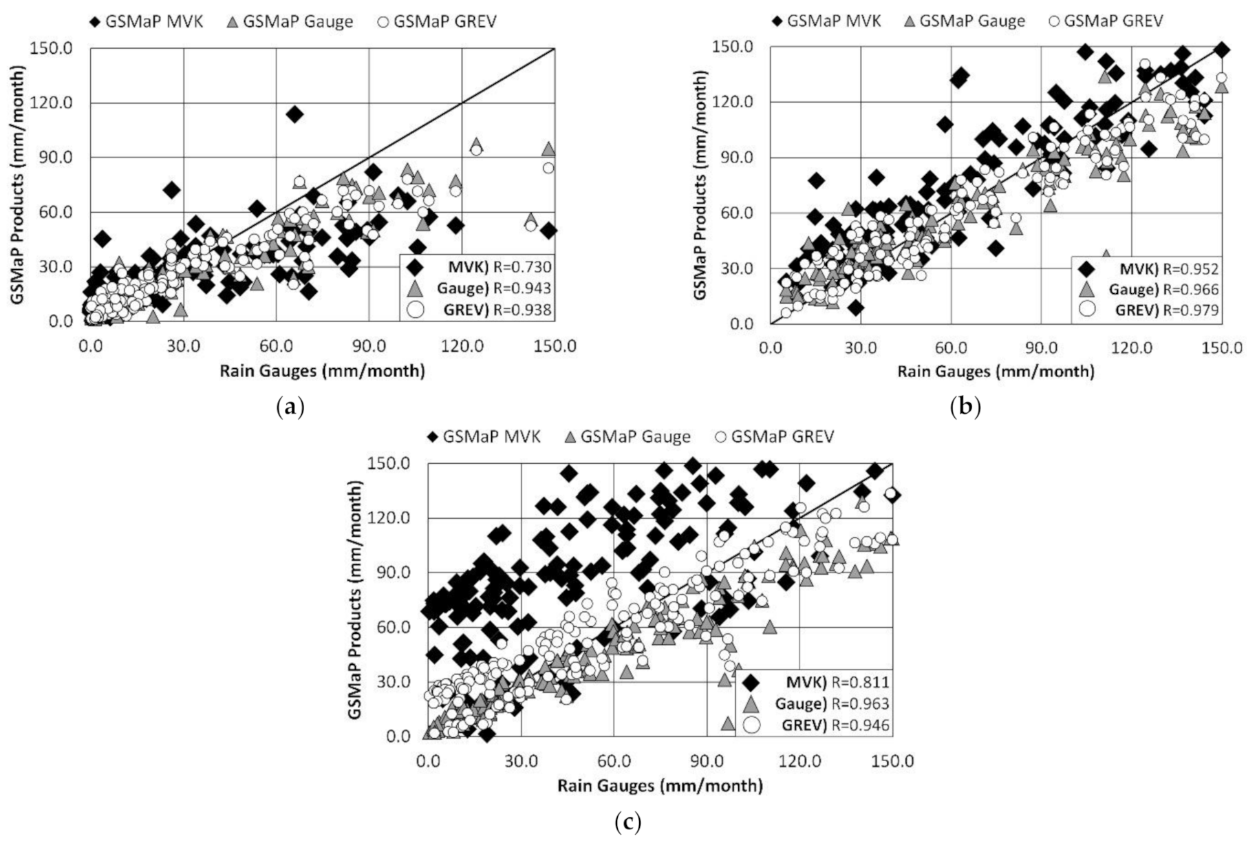
In
Figure 7, GSMaP_MVK presents the poorest results in the study basins. This product shows a slight overestimation of values less than 40 mm/month. Furthermore, this product presents an underestimation of values higher than 41 mm/month in the Altiplano basin. In the Amazon and La Plata basins, GSMaP_MVK shows overestimates with varying intensities. In
Figure 7b, the product presents a slight overestimation in comparison to rain gauges; however, in
Figure 7c, the overestimation is much higher. These results may be explained by the presence of rain gauges as the Amazon basin has a lower rain gauge density than the La Plata basin.
In the case of GSMaP_Gauge, the product shows better results in two of the three basins: Altiplano (
Figure 7a) and La Plata (
Figure 7c). In the Altiplano basin, the product exhibits deviations in values less than 40 mm/month and tends to underestimate higher values, similar to GSMaP_MVK. In the Amazon and La Plata basins, the variations show similar characteristics to those of GSMaP_MVK; these variations are higher in the La Plata basin than in the Amazon basin.
By comparison, the GSMaP_GREV product shows varied accuracy. In terms of its low values, the product presents slight variability in the three basins. Precipitation estimates for the Altiplano basin (
Figure 7a) show a greater underestimation compared to the value of the rain gauges, a characteristic similar to the other products. In the case of the Amazon basin (
Figure 7b), the variation of this product is similar to GSMaP_Gauge, however, the underestimation values of GSMaP_MVK are slightly less than the previous product. The Amazon basin is the only one in which this product shows better results. In the La Plata basin (
Figure 7c), the GSMaP_GREV represents a greater underestimation than the other products.
To choose the best GSMaP product group, monthly statistical indicators were selected, as shown in
Table 1. The R
2 and R values of the Altiplano and La Plata basins show better results with the GSMaP_Gauge, however, in the case of the Amazon basin the superior product is GSMaP_GREV. In terms of average ratios and accumulated bias, the Altiplano and Amazon basins favor the same GSMaP products as the previous metrics. In the La Plata basin, however, the GSMaP products show different values of ratio and bias. In the case of ratio values, the GSMaP_Gauge has an average underestimation of 16.8%, but GSMaP_GREV has the lowest accumulated bias of 137.3 mm. Finally, the indicators relating to data variations show the same superior products in the case of the Altiplano and Amazon basins (GSMaP_Gauge and GSMaP_GREV respectively).
Overall, the GSMaP_Gauge product shows better results in 11 out of 21 indicators, compared to GSMaP_GREV with 10 out of 21.
With the above analysis, we proceeded to analyze methods of generation in the GSMaP_Gauge and CHIRPS products. These products include some kind of rain-gauge adjustment.
3.2. Results of the Validation of Combination Methodology
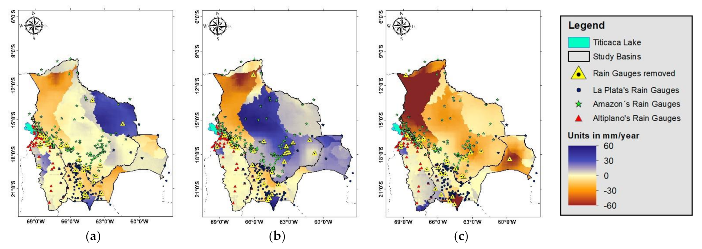
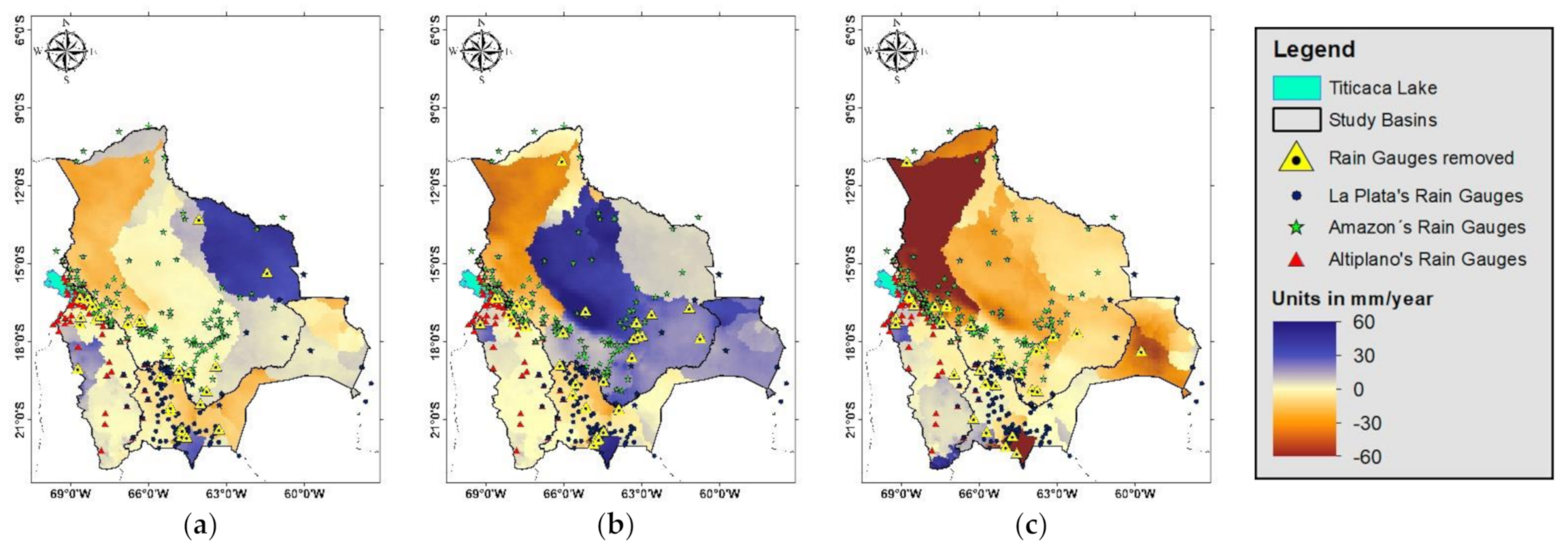
An analysis of the combined methodology was carried out to determine the possibility of generating products with the fewest rain gauges. This study attempted to generate new precipitation products with 90% of rain gauges. The remaining 10% were selected randomly and removed; ten cases were generated with this characteristic using sub-basins as a unit of analysis.
Figure 8 and
Figure 9 introduce three examples of GS and CH bias maps using 90% of rain gauges in relation to a rainfall map. In
Figure 8a and
Figure 9a, the basins show an overestimation of up to 30 mm/year, in particular in the east of the Amazon basin and the south of La Plata basin. The western area of the Amazon basin exhibits a slight underestimation of 15 mm/year.
Figure 8b and
Figure 9b show an overestimation in the central region of the Amazon basin, with values around 30 to 45 mm/year, and underestimation values in the western region of the Amazon basin increased.
Figure 8c and
Figure 9c display a large underestimation in the western zone of the Amazon basin, with values of around 60 mm/year, with an overall underestimation trend across the Amazon basin. The difference between the GS and CH products is mainly in terms of precipitation patterns.
Table 2 shows a summary of the statistical indicators for the GS product and an average of the generated products using 90% of the rain gauges. In this example, the GS products present better results compared to the average products. The determination and correlation coefficients are similar in the Altiplano and Amazon basins. The accumulated bias, MAE, and RMSE in Amazon basin show the highest values compared to the other basins. However, the NSE value in Amazon basin presents the lowest value for this group.
Table 3 shows similar values compared to the previous table. The differences between the values of these products are slight; the three basins present similar determination and correlation coefficients between GS and the average products. The average products’ accumulated bias, MAE, RMSE, and NSE also have similar values to the GS statistical indicators.
Our results validate that the generation methodology can be successfully used with 90% of the rain gauges in the country. Furthermore, these results suggest that the Amazon basin shows some peculiarities concerning precipitation data.
3.3. Generated Products
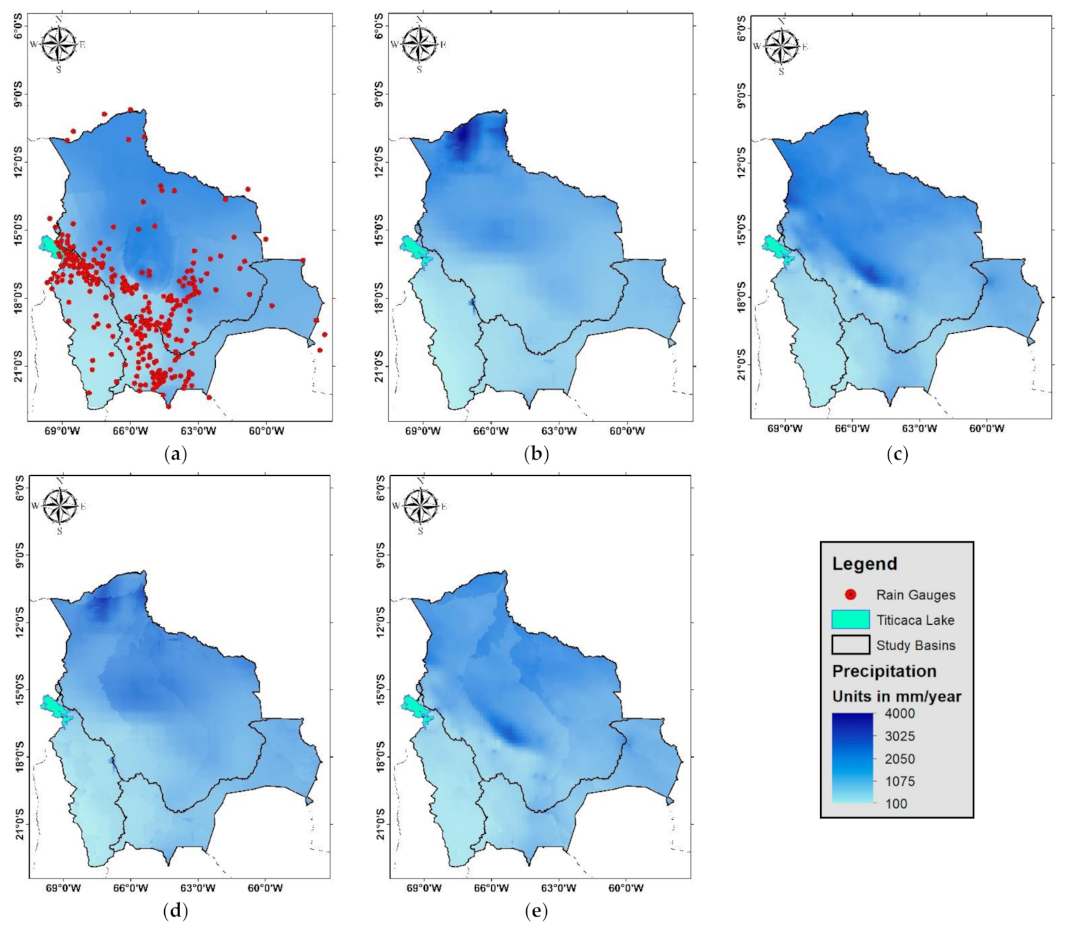
Following a comparison of the GSMaP data and combination method, we then considered the analysis of SBP products and combined products.
Figure 10 shows the precipitation map of initial precipitation products and the combined products in Bolivia. The GSMaP product (
Figure 10b) shows an overestimation in the northern zone of the Amazon basin in relation to the rain gauges and CHIRPS precipitation maps, with an overestimated precipitation value of around 3500 to 4000 mm/year. CHIRPS also presents a slight overestimation in the central part of the same basin (
Figure 10c), with a value of around 2800 to 3025 mm/year. GS and CH were the products generated in this study, based on GSMaP_Gauge and CHIRPS respectively. The GS and the CH products (
Figure 10d,e) show a similar spatial distribution to the map of rain gauges (
Figure 10a), but these products retain the characteristics of the initial SBPs.
The combined products appear to show a similar spatial resolution compared to the rain gauges’ map; however, this aspect of the data needs to be analyzed statistically. The scatter plots in
Figure 11 show an improvement in the SBP data after combining the products. In all cases, the satellite products present variations; however, the combined products present a closer approximation to the rain gauge data. The values of the combined products are higher, at 0.99, with a slight difference between GS and CH. However, the Amazon basin shows varied value underestimates in the case of the combined products. In the three study basins, CHIRPS presents better results than GSMaP, which may account for the slight difference between the GS and CH products.
In the case of the Altiplano basin, the CH product shows coefficient values closer to 1, meaning that the precipitation data of this product is closest to the values of the rain gauges (see
Table 4 below). However, the average ratio shows CH as an underestimating product with a value of 14.2%. For this indicator, CHIRPS presents a better result with a 0.6% underestimation value. In terms of their accumulated bias, GS and CH both present similar values. Based on the variation indicators (MAE, RMSE, and NSE), the generated products from this study show better results than the original SBPs.
The Amazon basin coefficients show similar characteristics to the Altiplano basin. In the examples of ratio and bias, CHIRPS is shown as the better product with an overestimation of 1.1% of average ratio and a difference of 43.5 mm accumulated bias over the selected period, and it can be seen in
Table 4. GS presents an accumulated bias of 77.4 mm while CH presents an accumulated bias of 98.4 mm. In the case of NSE, the CHIRPS dataset presents a better result.
In the La Plata basin, the determination and correlation coefficients show better results in the CH product. The bias of CH is the least in this basin with a 15.8 mm accumulation value, whereas CHIRPS has a better ratio with a 3.2% overestimation value. In terms of the variation indicators, CH is the better product.
In general, it can be seen that the generated products show better results than the SBPs used in their generation.
Table 5 shows the percentage of these improvements; the generated product based on GSMaP presents better results overall.
The basin with the highest improvement percentage is Altiplano with a 7.17% average. The basin with the smallest improvement percentage is the Amazon with 2.72%; however, this result may be affected by the rain gauge density in this basin.
3.4. Applicability of Combined Products in Distributed Hydrological Modeling
Based on the above metrics, the combined products (GS and CH) show a close similarity to the rain gauges’ data. However, to further validate these outputs, it is necessary to check integration with hydrological models. In this study, we used a simple equation to define the hydrological flow, see Equation 2 from the methodology section.
For comparison, we used BHSB data from 2012 and 2018. Both BHSB datasets are based on different precipitation data; in the case of the 2012 version, the study employed rain gauges and TRMM precipitation data [
26], whereas, in the 2018 version, Gridded Meteorological Ensemble Tool data were used [
22].
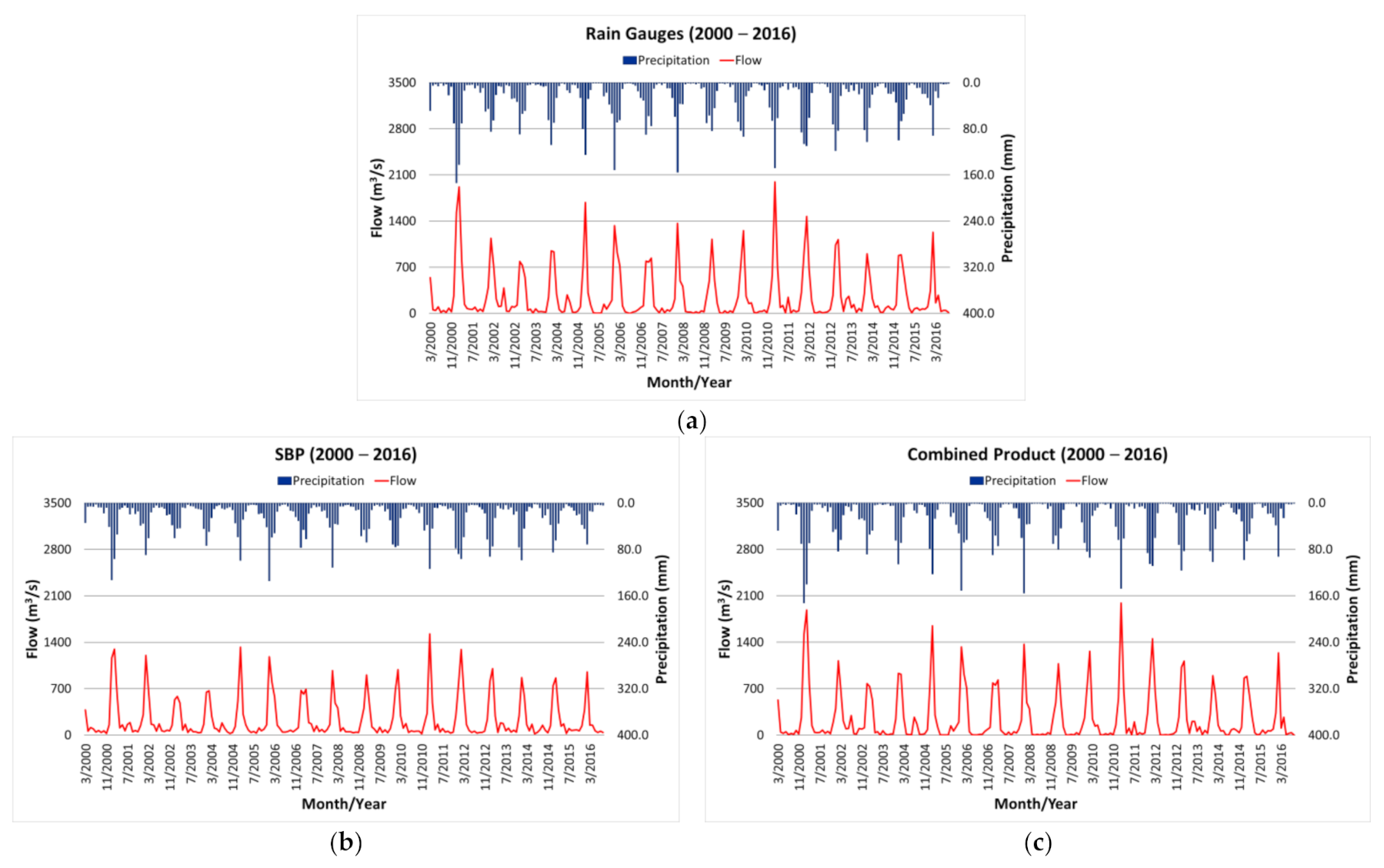
Figure 12 shows the calculated precipitation flow in the Altiplano basin for rain gauges, satellite-based products, and combined products. For SBPs (
Figure 12b), the precipitation and the flow values are underestimates compared to rain gauges. In contrast, the combined products (
Figure 12c) show similar precipitation and flow values in general. The precipitation data from the combined products show an underestimation during the months of June to October.
Table 6 shows some hydrological constants relating to precipitation and flow. The precipitation products under analysis use data from different time periods; BHSB 2012 has 32 years of data, BHSB 2018 has 36 years, whereas the tools used in this study cover a period of 16 years.
For the generation of constants, the runoff data from BHSB 2018 were used. The basins in this study show annual runoff coefficient values of 0.16 (Altiplano basin), 0.41 (Amazon basin), and 0.30 (La Plata basin). For BHBS 2012 and 2018, the hydrological constant was obtained directly based on the value listed in their documentation.
In the case of the Altiplano basin, BHSB 2012 and 2018 show relatively similar hydrological constant values, however, the selected precipitation products in this study present lower values. The value for the Amazon basin is somewhat different compared to the Altiplano basin, which may result from differences in precipitation, runoff, and surface area. For the La Plata basin, the hydrological constants of the products in this study yield an overestimate compared to BHSB 2018 data. This result occurred because the approach used in terms of implementation and generation of rain gauge maps was different from that of BHSB; another potential factor was the hydrological model used.
4. Discussion
Bolivia has three major basins: Altiplano (151,722 km2), Amazon (720,792 km2), and La Plata (225,492 km2). These basins show elevation values between 200 and 5000 m.a.s.l. In these basins, three main ecological systems are present: highlands, valleys, and lowlands. For the study, three goals were set: evaluation of GSMaP products, analysis of the combination approach, and evaluation of generated products using this method.
The GSMaP products selected for analysis were: GSMaP_MVK (the first version of the product), GSMaP_Gauge (standard version), and GSMaP_GREV (a revised version of the previous product). GSMaP_MVK gave significant precipitation overestimates in the southern part of the Amazon basin and the northeastern part of La Plata basin compared to GSMaP_Gauge and GSMaP_GREV. In general, the GSMaP products show consistently close correlation coefficient values between 0.907 and 0.979. The GSMaP products have an RMSE value of around 15.9 to 35.1. GSMaP_Gauge performed best in the Altiplano basin, whereas GSMaP_GREV was best in the Amazon Basin. In the La Plata basin, the GSMaP_Gauge was best in terms of R2, R, and the average ratio, whereas the GSMaP_GREV performed best for the accumulated bias and RMSE values. As a result, the GSMaP_Gauge and CHIRPS data were selected subsequently to generate the combined products.
For the scheme proposed here, it was necessary to employ both rain gauge data and SBP data. Consequently, the analysis considered two aspects: the generation of GSMaP and CHIRPS’ combined products, and the importance of rain gauge locations. To test the latter of these metrics, the combined products were tested with 90% of the available rain gauges. The unused 10% of rain gauges were randomly selected, and this operation was carried out 10 times. The results of these analyses showed a consistent spatial distribution, with only slight differences between them. In terms of analyzing their statistical indicators, the correlation coefficient values were highly consistent, with values between 0.9883 to 0.9990 for GSMaP products and 0.9893 to 0.9994 for CHIRPS products. The combined products, therefore, showed similar results despite the different locations of rain gauges.
The combined approach used in this study yielded acceptable results, however, the Amazon basin showed the poorest results of the three basins. This is possibly due to the density of rain gauges; in the La Plata and Altiplano Basins, the density is around 1806 to 2013 km2 per station, whereas the Amazon basin has a much sparser density of 4027 km2 per station. The presence of rain gauges used in the combination method can be a factor in obtaining better results. Using 90% of the rain gauges, it was possible to generate acceptable results with the combined precipitation products. Having validated the approach in this way, it would be possible in future to continue removing rain gauges to test the limit at which this methodology can no longer generate acceptable combined products.
The combined products also show improvements over the SBP. In terms of their spatial resolution, the combined products of GSMaP (GS) and CHIRPS (CH) show similar values compared to the rain gauge map. However, these combined products retain some characteristics of the SBP product used in their generation. In the scatter plots and time series, the Amazon basin presents the worst results in relation to the other study basins; in this area, the correlation coefficient is around 0.9902 to 0.9910, compared to 0.9951 to 0.9997 in the other basins. Although the combined products in the Amazon basin exhibit a considerable underestimate of precipitation, the improvement percentage values nonetheless indicate that the combined products perform better than the original SBP products. GS shows better improvement percentages, with values of 10.96%, 4.91%, and 6.36% for Altiplano, Amazon, and La Plata basins respectively. However, CH yields values of 3.37%, 0.52%, and 5.80% in the same basins. Therefore, it can be concluded that although the combination methodology presents an acceptable improvement for both datasets, using the GSMaP_Gauge product generates a better overall result. Our study also indicates that the generated products can be employed in semi-distributed hydrological models.
The results of this study present an alternative method for generating distributed precipitation products in situations where SBP products do not show acceptable values in comparison with rain gauges. Compared to the initial SBPs employed in this study, the combined products showed similar precipitation and flow values in comparison to rain gauge data. In comparison to BHSB, the hydrological constants of the study products show considerable variations. This can be accounted for by differences in the generation of precipitation maps, the hydrological model employed, and the period of data used.
5. Conclusions
Among the GSMaP products studied, GSMaP_Gauge showed better results in comparison to other versions. This product and CHIRPS were the SBPs selected to generate a combined product with the rain gauge data of a local network. The methodology employed was based on a series of iterations.
The combined products GS (based on GSMaP) and CH (based on CHIRPS) demonstrate better results than the original SBPs, with an average improvement of around 5%.
The proposed validation method showed that the greater the number of local rain gauges, the better the performance of the combined method. Ten percent of the available rain gauges in the country were randomly removed and high-quality results were still obtained.
A water budget exercise demonstrated that hydrographs can be readily obtained, as well as estimates of water availability in the country. Using the GS product from this study, the yearly water availability for Bolivia reached 445,858 hm3.
In conclusion, the database generated in this study can be used by the scientific community and the public for different hydrological applications such as precipitation time-series analysis, distributed hydrological modeling, and water assessment at a sub-basin scale within Bolivia.
Finally, the proposed methodology here can be applied in other countries to enhance spatial and temporal resolution of precipitation datasets.
Author Contributions
Conceptualization, J.U. and O.S.; methodology, J.U. and O.S.; software, J.U.; validation, J.U., O.S. and T.K.; formal analysis, J.U. and O.S.; investigation, J.U. and O.S.; resources, J.U. and O.S.; data curation, T.K.; writing—original draft preparation, J.U.; writing—review and editing, J.U. and O.S.; visualization, J.U.; supervision, O.S. and T.K.; project administration, O.S. All authors have read and agreed to the published version of the manuscript.
Funding
This research received no external funding.
Data Availability Statement
Acknowledgments
This research has been supported by the 2nd Research Announcement on the Earth Observations of the Japan Aerospace Exploration Agency (JAXA) for data sharing of GSMaP_ MVK, GSMaP_Gauge and GSMaP_GREV in them version 6. We would like to appreciate Tomoko Tashima of JAXA/EORC for her support in the revision of GSMAP datasets. We also appreciate the effort and support of the editor and anonymous reviewers who enabled the improvement of this paper.
Conflicts of Interest
The authors declare that there are no conflicts of interest regarding the publication of this paper.
References
- Olaoye, I.A.; Confesor, R.B., Jr.; Ortiz, J.D. Effect of projected land use and climate change on water quality of old woman creek watershed, Ohio. Hydrology 2021, 8, 62. [Google Scholar] [CrossRef]
- Lee, J.; Kim, B. Scenario-Based real-time flood prediction with logistic regression. Water 2021, 13, 1191. [Google Scholar] [CrossRef]
- Hamdan, A.N.A.; Almuktar, S.; Scholz, M. Rainfall-Runoff modeling using the HEC-HMS model for the Al-Adhaim river catchment, northern Iraq. Hydrology 2021, 8, 58. [Google Scholar] [CrossRef]
- Fraga, I.; Cea, L.; Puertas, J. Effect of rainfall uncertainty on the performance of physically based rainfall–runoff models. Hydrol. Process. 2019, 33, 160. [Google Scholar] [CrossRef] [Green Version]
- Chen, T.; Ren, L.; Yuan, F.; Yang, X.; Jiang, S.; Tang, T.; Liu, Y.; Zhao, C.; Zhang, L. Comparison of spatial interpolation schemes for rainfall data and application in hydrological modeling. Water 2017, 9, 342. [Google Scholar] [CrossRef] [Green Version]
- Liu, S.; Li, Y.; Pauwels, V.; Walker, J. Impact of rain gauge quality control and interpolation on streamflow simulation: An application to the warwick catchment, Australia. Front. Earth Sci. 2018, 5, 114. [Google Scholar] [CrossRef] [Green Version]
- Ryu, S.; Song, J.; Kim, Y.; Sung-Hwa, J.; Younghae, D.; GyuWon, L. Spatial interpolation of gauge measured rainfall using compressed sensing. Asia Pac. J. Atmos. Sci. 2021, 57, 331. [Google Scholar] [CrossRef] [Green Version]
- Blacutt, L.A.; Herdies, D.L.; de Goncalves, L.G.; Vila, D.A.; Andrade, M. Precipitation comparison for the CFSR, MERRA, TRMM3B42 and combined scheme datasets in Bolivia. Atmos. Res. 2015, 163, 117. [Google Scholar] [CrossRef] [Green Version]
- World Meteorological Organization. Review of Requirements for Area-Averaged Precipitation Data, Surface-Based and Space-Based Estimation Techniques, Space and Time Sampling, Accuracy and Error; Data Exchange: Boulder, CO, USA, 1985; Available online: https://library.wmo.int/doc_num.php?explnum_id=9228 (accessed on 20 May 2021).
- Kubota, T.; Shige, S.; Hashizume, H.; Aonashi, K.; Takahashi, N.; Seto, S.; Hirose, M.; Takayabu, Y.N.; Ushio, T.; Nakagawa, K.; et al. Global precipitation map using satellite-borne microwave radiometers by the gsmap project: Production and validation. IEEE Trans. Geosci. Remote Sens. 2007, 45, 2259. [Google Scholar] [CrossRef]
- Kubota, T.; Aonashi, K.; Ushio, T.; Shige, S.; Takayabu, Y.N.; Kachi, M.; Arai, Y.; Tashima, T.; Masaki, T.; Kawamoto, N.; et al. Global satellite mapping of precipitation (GSMaP) products in the GPM era. Satell. Precip. Meas. 2020, 67, 355. [Google Scholar] [CrossRef]
- Ushio, T.; Sasashige, K.; Kubota, T.; Shige, S.; Okamoto, K.; Aonashi, K.; Inoue, T.; Takahashi, N.; Iguchi, T.; Kachi, M.; et al. A kalman filter approach to the global satellite mapping of precipitation (GSMaP) from combined passive microwave and infrared radiometric data. J. Meteor. Soc. 2009, 87, 137. [Google Scholar] [CrossRef] [Green Version]
- Funk, C.; Peterson, P.; Landsfeld, M.; Pedreros, D.; Verdin, J.; Shukla, S.; Husak, G.; Rowland, J.; Harrison, L.; Hoell, A.; et al. The climate hazards infrared precipitation with stations—A new environmental record for monitoring extremes. Sci. Data 2015, 2. [Google Scholar] [CrossRef] [PubMed] [Green Version]
- Funk, C.; Peterson, P.; Landsfeld, M.; Davenport, F.; Becker, A.; Schneider, U.; Pedreros, D.; McNally, A.; Arsenault, K.; Harrison, L.; et al. Algorithm and data improvements for version 2.1 of the Climate hazards center’s infrared precipitation with stations data set. Satell. Precip. Meas. Adv. Glob. Chang. Res. 2020, 67, 409. [Google Scholar] [CrossRef]
- Takido, K.; Saavedra, O.; Ryo, M.; Tanuma, K.; Ushio, T.; Kubota, T. Spatiotemporal evaluation of the gauge-ajusted satellite mapping of precipitation at the basin scale. J. Meteorol. Soc. 2016, 94, 185. [Google Scholar] [CrossRef] [Green Version]
- Tian, Y.; Peters-Lidard, C.D. A global map of uncertainties in satellite-based precipitation measurements. Geophys. Res. Lett. 2010, 37. [Google Scholar] [CrossRef]
- Mahmoud, M.T.; Mohammed, S.A.; Hamouda, M.A.; Mohamed, M.M. Impact of topography and rainfall intensity on the accuracy of imerg precipitation estimates in an arid region. Remote Sens. 2021, 13, 13. [Google Scholar] [CrossRef]
- Mahmund, M.R.; Hashim, M.; Reba, M. How effective is the new generation of gpm satellite precipitation in characterizing the rainfall variability over malaysia? Asia Pac. J. Atmos Sci. 2017, 53, 375. [Google Scholar] [CrossRef]
- Zhao, Y.; Xie, Q.; Lu, Y.; Hu, B. Hydrologic evaluation of trmm multisatellite precipitation analysis for nanliu river basin in humid southwestern China. Sci. Rep. 2017, 7, 2470. [Google Scholar] [CrossRef] [Green Version]
- Nwachukwu, P.N.; Satge, F.; Yacoubi, S.E.; Pinel, S.; Bonnet, M.-P. From TRMM to GPM: How reliable are satellite-based precipitation data across nigeria? Remote Sens. 2020, 12, 3964. [Google Scholar] [CrossRef]
- Yanto; Livneh, B.; Rajagopalan, B. Development of a gridded meteorological dataset over Java island, Indonesia 1985–2014. Sci. Data 2017, 4, 170072. [Google Scholar] [CrossRef] [PubMed] [Green Version]
- Ministerio de Medio Ambiente y Agua. Balance Hídrico Superficial de Bolivia (1980–2016); Stockholm Environment Institute; Servicio Nacional de Meteorologia e Hidrologia (SENAMHI); Instituto de Hidraulica e Hidrologia de la Universidad Mayor de San Andres (IHH/UMSA); Laboratorio de Hidraulica de la Universidad Mayor de San Simon (LH/UMSS): La Paz, Bolivia, 2018.
- Mega, T.; Ushio, T.; Matsuda, T.; Kubota, T.; Kachi, M.; Oki, R. Gauge-Adjusted global satellite mapping of precipitation. IEEE Trans. Geosci. Remote Sens. 2019, 57, 1928. [Google Scholar] [CrossRef]
- Ureña, J.; Saavedra, O. Evaluation of satellite based precipitation products at key basins in Bolivia. Asia Pac. J. Atmos. Sci. 2020, 56, 641. [Google Scholar] [CrossRef]
- Villazón, M.; Willems, P. Filling Gaps and Daily Disaccumulation of Precipitation Data for Rainfall-Runoff Model; BALWOIS: Ohrid, Macedonia, 2010; Available online: https://www.researchgate.net/publication/228804071_Filling_gaps_and_Daily_Disaccumulation_of_Precipitation_Data_for_Rainfall-runoff_model#fullTextFileContent (accessed on 20 May 2021).
- Ministerio de Medio Ambiente y Agua. Balance Hídrico Superficial de Bolivia (1980–2012); Programa de Desarrollo Agropecuario Sustentable (GIZ/PROAGRO): La Paz, Bolivia, 2012.
Figure 1.
(a) Hydrological and orographic map of Bolivia; (b) three major basins in Bolivia.
Figure 1.
(a) Hydrological and orographic map of Bolivia; (b) three major basins in Bolivia.
Figure 2.
(a) Mean multi-year precipitation map of Bolivia for 2001–2015 interpolation; (b) available rain gauges’ location in Bolivia during 1980–2016.
Figure 2.
(a) Mean multi-year precipitation map of Bolivia for 2001–2015 interpolation; (b) available rain gauges’ location in Bolivia during 1980–2016.
Figure 3.
Sub-basins using Pfafstetter coding system (level 3): (a) Altiplano, (b) Amazon and (c) La Plata basins.
Figure 3.
Sub-basins using Pfafstetter coding system (level 3): (a) Altiplano, (b) Amazon and (c) La Plata basins.
Figure 4.
Flow chart process to obtain the combined product using satellite-based precipitation (SBP) and the rain gauge network. Source: Adapted from Ureña and Saavedra [
2].
Figure 4.
Flow chart process to obtain the combined product using satellite-based precipitation (SBP) and the rain gauge network. Source: Adapted from Ureña and Saavedra [
2].
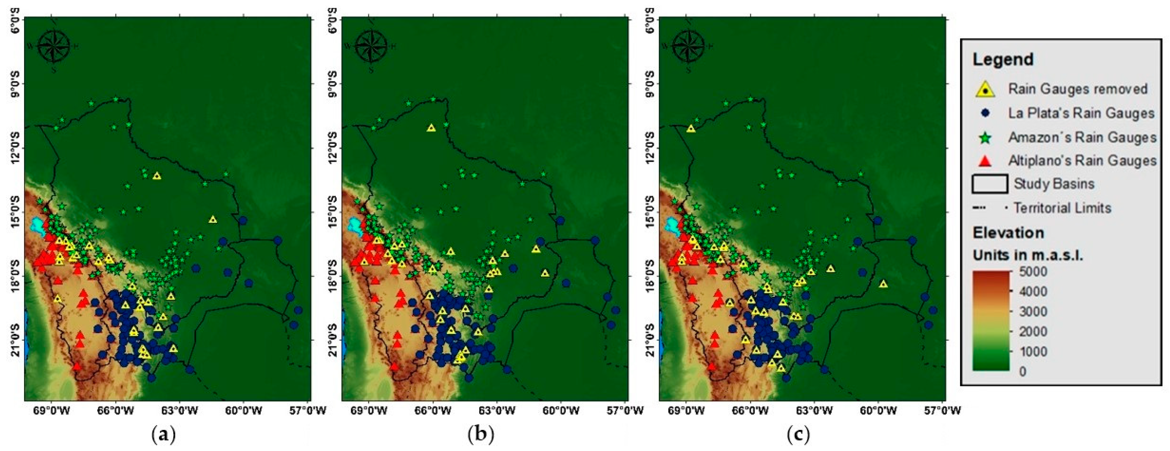
Figure 5.
Three scenarios where 10% of rain gauges were removed and used as a control for validation: (a) Case1, (b) Case 2 and (c) Case 3.
Figure 5.
Three scenarios where 10% of rain gauges were removed and used as a control for validation: (a) Case1, (b) Case 2 and (c) Case 3.
Figure 6.
Average annual precipitation maps for the period 2001–2015 of: (a) Global Satellite Mapping of Precipitation (GSMaP) moving vector by Kalman-filter (MVK), (b)GSMaP Gauge and (c) GSMaP GREV.
Figure 6.
Average annual precipitation maps for the period 2001–2015 of: (a) Global Satellite Mapping of Precipitation (GSMaP) moving vector by Kalman-filter (MVK), (b)GSMaP Gauge and (c) GSMaP GREV.
Figure 7.
Monthly scatter plots data for the period 2000–2015 for: (a) Altiplano basin, (b) Amazon basin and (c) La Plata basin.
Figure 7.
Monthly scatter plots data for the period 2000–2015 for: (a) Altiplano basin, (b) Amazon basin and (c) La Plata basin.
Figure 8.
Average annual bias maps of combined products employed 90% for three cases in the period 2001–2015 of GS products: (a) Case1, (b) Case 2 and (c) Case 3.
Figure 8.
Average annual bias maps of combined products employed 90% for three cases in the period 2001–2015 of GS products: (a) Case1, (b) Case 2 and (c) Case 3.
Figure 9.
Average annual bias maps of combined products employed 90% for three cases in the period 2001–2015 of CH products: (a) Case1, (b) Case 2 and (c) Case 3.
Figure 9.
Average annual bias maps of combined products employed 90% for three cases in the period 2001–2015 of CH products: (a) Case1, (b) Case 2 and (c) Case 3.
Figure 10.
Average annual precipitation maps for the period 2001–2015 of: (a) rain gauges, (b) GSMaP_Gauge, (c) CHIRPS, (d) GS and (e) CH.
Figure 10.
Average annual precipitation maps for the period 2001–2015 of: (a) rain gauges, (b) GSMaP_Gauge, (c) CHIRPS, (d) GS and (e) CH.
Figure 11.
Monthly scatter plots of the SBP products (left) and combined products (right) for: (a) Altiplano, (b) Amazon and (c) La Plata basins.
Figure 11.
Monthly scatter plots of the SBP products (left) and combined products (right) for: (a) Altiplano, (b) Amazon and (c) La Plata basins.
Figure 12.
Precipitation time series and river discharge of Altiplano basin for: (a) rain gauge, (b) average satellite-based product and (c) average combined product.
Figure 12.
Precipitation time series and river discharge of Altiplano basin for: (a) rain gauge, (b) average satellite-based product and (c) average combined product.
Table 1.
Statistics indicators for GSMaP product in the study basins.
Table 1.
Statistics indicators for GSMaP product in the study basins.
| | Altiplano Basin | Amazon Basin | La Plata Basin |
|---|
Statistics
Indicators | MVK | Gauge | GREV | MVK | Gauge | GREV | MVK | Gauge | GREV |
| Determination Coefficient (R2) | 0.533 | 0.888 | 0.879 | 0.906 | 0.932 | 0.959 | 0.657 | 0.927 | 0.895 |
Correlation
Coefficient (R) | 0.730 | 0.943 | 0.938 | 0.952 | 0.966 | 0.979 | 0.811 | 0.963 | 0.946 |
| Average Ratio (%) | 166.8 | 130.3 | 137.7 | 112.6 | 94.0 | 95.4 | 253.9 | 83.2 | 119.7 |
| Accumulate Bias (mm) | 157.8 | 97.2 | 191.7 | 185.8 | 229.0 | 183.2 | 461.7 | 177.4 | 137.3 |
| Mean Absolute Error (MAE) | 15.7 | 9.5 | 10.1 | 20.6 | 21.6 | 18.5 | 44.0 | 15.6 | 16.0 |
| Root Mean Square Error (RMSE) | 26.6 | 16.1 | 16.8 | 27.3 | 30.2 | 24.0 | 50.2 | 23.7 | 19.9 |
| Nash and Sutcliffe Efficiency (NSE) | 0.45 | 0.80 | 0.78 | 0.88 | 0.85 | 0.91 | 0.17 | 0.81 | 0.87 |
Table 2.
Statistics Indicators for products based in GSMaP_Gauge in the study.
Table 2.
Statistics Indicators for products based in GSMaP_Gauge in the study.
| | Altiplano Basin | Amazon Basin | La Plata Basin |
|---|
Statistics
Indicators | GS | Average 90% | GS | Average 90% | GS | Average 90% |
| Determination Coefficient (R2) | 0.9979 | 0.9958 | 0.9805 | 0.9802 | 0.9903 | 0.9862 |
Correlation
Coefficient (R) | 0.9990 | 0.9979 | 0.9902 | 0.9901 | 0.9951 | 0.9931 |
| Average Ratio (%) | 88.2 | 88.0 | 86.6 | 85.8 | 95.5 | 95.3 |
| Accumulate Bias (mm) | 12.4 | 11.9 | 77.4 | 90.7 | 21.3 | 24.2 |
| Mean Absolute Error (MAE) | 1.2 | 1.6 | 7.5 | 8.7 | 1.8 | 2.9 |
| Root Mean Square Error (RMSE) | 2.0 | 2.6 | 13.3 | 13.8 | 5.7 | 6.7 |
| Nash and Sutcliffe Efficiency (NSE) | 0.9970 | 0.9950 | 0.9709 | 0.9687 | 0.9892 | 0.9848 |
Table 3.
Statistics indicators for products based on Climate Hazards Group Infrared Precipitations with Stations (CHIRPS) in the study.
Table 3.
Statistics indicators for products based on Climate Hazards Group Infrared Precipitations with Stations (CHIRPS) in the study.
| | Altiplano Basin | Amazon Basin | La Plata Basin |
|---|
Statistics
Indicators | CH | Average 90% | CH | Average 90% | CH | Average 90% |
| Determination Coefficient (R2) | 0.9989 | 0.9962 | 0.9821 | 0.9812 | 0.9994 | 0.9926 |
Correlation
Coefficient (R) | 0.9994 | 0.9981 | 0.9910 | 0.9905 | 0.9997 | 0.9963 |
| Average Ratio (%) | 85.8 | 86.4 | 84.2 | 84.1 | 95.5 | 95.4 |
| Accumulate Bias (mm) | 13.4 | 12.2 | 98.4 | 106.6 | 15.8 | 20.1 |
| Mean Absolute Error (MAE) | 1.2 | 1.6 | 8.6 | 9.6 | 1.4 | 2.6 |
| Root Mean Square Error (RMSE) | 1.6 | 2.5 | 13.9 | 14.4 | 1.9 | 4.6 |
| Nash and Sutcliffe Efficiency (NSE) | 0.9979 | 0.9952 | 0.9680 | 0.9671 | 0.9988 | 0.9915 |
Table 4.
Statistics Indicators for SBP products and combined products.
Table 4.
Statistics Indicators for SBP products and combined products.
| | Altiplano Basin | Amazon Basin | La Plata Basin |
|---|
Statistics
Indicators | GSMaP | GS | CHIRPS | CH | GSMaP | GS | CHIRPS | CH | GSMaP | GS | CHIRPS | CH |
Determination
Coefficient (R2) | 0.8885 | 0.9979 | 0.9652 | 0.9989 | 0.9324 | 0.9805 | 0.9770 | 0.9821 | 0.9273 | 0.9903 | 0.9414 | 0.9994 |
Correlation
Coefficient (R) | 0.9426 | 0.9990 | 0.9824 | 0.9994 | 0.9656 | 0.9902 | 0.9884 | 0.9910 | 0.9629 | 0.9951 | 0.9703 | 0.9997 |
| Average Ratio (%) | 130.3 | 88.2 | 99.4 | 85.8 | 94.0 | 86.6 | 101.1 | 84.2 | 83.2 | 95.5 | 103.2 | 95.5 |
| Accumulated Bias (mm) | 97.2 | 12.4 | 36.9 | 13.4 | 229.0 | 77.4 | 43.5 | 98.4 | 177.4 | 21.3 | 56.6 | 15.8 |
| Mean Absolute Error (MAE) | 9.5 | 1.2 | 5.1 | 1.2 | 21.6 | 7.5 | 9.3 | 8.6 | 15.6 | 1.8 | 8.9 | 1.4 |
| Root Mean Square Error (RMSE) | 16.1 | 2.0 | 7.3 | 1.6 | 30.2 | 13.3 | 12.2 | 13.9 | 23.7 | 5.7 | 13.7 | 1.9 |
| Nash and Sutcliffe Efficiency (NSE) | 0.8002 | 0.9970 | 0.9589 | 0.9979 | 0.8503 | 0.9709 | 0.9755 | 0.9680 | 0.8148 | 0.9892 | 0.9377 | 0.9988 |
Table 5.
Improvement percentage of precipitation products.
Table 5.
Improvement percentage of precipitation products.
| Relation | Altiplano Basin | Amazon Basin | La Plata Basin | Average |
|---|
| GSMaP to GS | 10.96 | 4.91 | 6.36 | 7.41 |
| CHIRPS to CH | 3.37 | 0.52 | 5.80 | 3.23 |
| SBP to Combined | 7.17 | 2.72 | 6.08 | 5.32 |
Table 6.
Annual hydrological constant for precipitation products.
Table 6.
Annual hydrological constant for precipitation products.
| | Altiplano Basin | Amazon Basin | La Plata Basin |
|---|
| | Pr (mm) | Q (m3/s) | QSp
(L/s-km2) | Volume (hm3) | Pr (mm) | Q (m3/s) | QSp
(L/s-km2) | Volume (hm3) | Pr (mm) | Q (m3/s) | QSp
(L/s-km2) | Volume (hm3) |
|---|
| BHSB 2012 | 351.9 | 345.6 | 2.3 | 10,899.1 | 1351.1 | 13813.3 | 19.4 | 435,615.3 | 696.2 | 1079.8 | 4.8 | 34,053.8 |
| BHSB 2018 | 496.5 | 370.3 | 2.4 | 11,677.9 | 1629.0 | 15367.8 | 21.3 | 484,646.1 | 713.8 | 1546.3 | 6.9 | 48,761.4 |
| Rain Gauges | 343.9 | 256.5 | 1.7 | 8089.4 | 1368.5 | 12910.3 | 17.9 | 407,137.6 | 810.9 | 1756.6 | 7.8 | 55,395.5 |
| GSMaP | 293.0 | 218.5 | 1.4 | 6891.4 | 1172.7 | 11063.1 | 15.3 | 348,892.4 | 634.2 | 1373.8 | 6.1 | 43,325.3 |
| CHIRPS | 322.3 | 240.4 | 1.6 | 7581.3 | 1399.3 | 13200.9 | 18.3 | 416,292.3 | 794.0 | 1720.0 | 7.6 | 54,245.0 |
| GS | 331.5 | 247.3 | 1.6 | 7796.3 | 1291.1 | 12180.1 | 16.9 | 384,119.3 | 789.6 | 1710.5 | 7.6 | 53,942.6 |
| CH | 330.5 | 246.5 | 1.6 | 7773.4 | 1270.2 | 11983.0 | 16.6 | 377,892.4 | 795.1 | 1722.4 | 7.6 | 54,319.4 |
| Publisher’s Note: MDPI stays neutral with regard to jurisdictional claims in published maps and institutional affiliations. |
© 2021 by the authors. Licensee MDPI, Basel, Switzerland. This article is an open access article distributed under the terms and conditions of the Creative Commons Attribution (CC BY) license (https://creativecommons.org/licenses/by/4.0/).


