Abstract
River system is critical for the future sustainability of our planet but is always under the pressure of food, water and energy demands. Recent advances in machine learning bring a great potential for automatic river mapping using satellite imagery. Surface river mapping can provide accurate and timely water extent information that is highly valuable for solid policy and management decisions. However, accurate large-scale river mapping remains challenging given limited labels, spatial heterogeneity and noise in satellite imagery (e.g., clouds and aerosols). In this paper, we propose a new multi-source data-driven method for large-scale river mapping by combining multi-spectral imagery and synthetic aperture radar data. In particular, we build a multi-source data segmentation model, which uses contrastive learning to extract the common information between multiple data sources while also preserving distinct knowledge from each data source. Moreover, we create the first large-scale multi-source river imagery dataset based on Sentinel-1 and Sentinel-2 satellite data, along with 1013 handmade accurate river segmentation mask (which will be released to the public). In this dataset, our method has been shown to produce superior performance (F1-score is 91.53%) over multiple state-of-the-art segmentation algorithms. We also demonstrate the effectiveness of the proposed contrastive learning model in mapping river extent when we have limited and noisy data.
1. Introduction
River system plays a crucial role in global carbon circulation, as it delivers the carbonaceous matter within the global ecosystem and maintains the connection between ocean and land [1,2]. Rivers are also important in many countries due to the increasing demand to supply drinking water, irrigation and farming practices and power generation. Hence, the capacity to accurately map large-scale rivers is urgently needed for making policy and management decisions.
With the recent development of the space remote sensing technology, satellite images become available over large regions (often at global scale), which enables large-scale surface area monitoring [3,4]. Many existing methods utilize pre-defined water indices, such as Normalized Difference Water Index (NDWI) [5] and Modified Normalized Difference Water Index (MNDWI) [6], which are computed from a subset of spectral bands. These indices are designed to enhance the water representation in contrast to other land covers based on the reflectance characteristics.
Recently, there is a growing interest in land cover mapping using machine learning algorithms including Support Vector Machine (SVM) [7], Random Forest (RF) [8] and deep learning-based image segmentation algorithms such as UNET [9] and Pspnet [10]. Compared with the water indices, these machine learning methods can better extract informative non-linear combinations of reflectance values from all the spectral bands that can reflect water extent [11,12]. Additionally, deep learning-based image segmentation methods often outperform pre-defined water indices and traditional pixel-wise machine learning algorithms due to their capacity to capture image-level information. In particular, these deep learning models use receptive fields to capture spatial dependencies across pixels and thus have a better chance at capturing informative patterns related to river shapes, compactness and surrounding land covers [13,14].
However, large-scale river mapping still remains a challenge due to several reasons [15,16,17,18]. Firstly, we often have limited labeled training samples due to the high cost associated with manual annotation through visual inspection. This become especially serious for training advanced deep learning models. Second, rivers located in different regions can have different water properties, catchment characteristics and surrounding land covers and thus show different reflectance spectral value in the satellite imagery [19]. Traditional machine learning methods that are trained from limited labeled samples collected from specific regions may not be able to generalize to other regions [20,21]. Third, given the nature of remote sensing imagery, the river area in the multi-spectral satellite images may be blocked by unpredictable noise such as aerosol and clouds, leading to missing information during the river mapping process [22,23].
To address these challenges, we propose a new machine learning method that combines multi-spectral data and synthetic aperture radar (SAR) data to jointly map the extent of rivers over large regions, the main idea of the proposed method is shown in Figure 1.
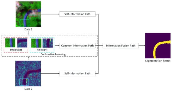
Figure 1.
The proposed contrastive learning based multi-source data segmentation structure. The segmentation result is generated using the self-information and common information, extracting from the multi-source data pair, including Data 1 and Data 2. For the common information extracting process, the contrastive learning idea is to minimize the relevant image information embedding between the same location multi-source data. Here, the relevant image information are extracted from multi-source data pair of same location and the irrelevant image information are extracted from multi-source data pair of different location. Thus, the common information path can be more focused on the clear area of the image (without aerosol and cloud) and can guide the segmentation process, along with the self-information extracted from each multi-source data.
The multi-spectral data can capture optical reflectance characteristics of different land covers while SAR data is more sensitive to surface structures and also less impacted by clouds and aerosols. We build a novel machine learning algorithm that can leverage supplementary strengths of these two types of data to improve the mapping performance. Our major innovation and contributions can be summarized as follows:
- We present a contrastive learning based multi-source satellite data segmentation structure for large-scale river mapping, as shown in Figure 1. To better extract representative patterns from limited and noisy data, we include the contrastive learning strategies, where the common information and self-information are extracted from the multi-source data and fused for the river segmentation.
- We create a large-scale multi-source river imagery dataset, which, to the best of our knowledge, is the first multi-source large-scale satellite dataset (with aligned multi-spectral data and SAR data) towards river mapping. The dataset contains multi-spectral data and SAR data for 1013 river sites that are distributed over the entire globe and handmade ground truth masks for these river sites.
- On our dataset, we have demonstrated the superiority of the proposed multi-source segmentation method over multiple widely used methods including water indices-based method, traditional machine learning approaches and deep learning approaches.
2. Materials and Methods
2.1. Study Area and Data
Aiming at the large-scale river mapping task, we first create a large-scale multi-source river imagery dataset, which to the best of our knowledge, is the first multi-source large-scale satellite dataset toward river mapping. This dataset contains 1013 image pairs of rivers based on Sentinel-1 and Sentinel-2 satellite and 1013 manually annotated river ground truth masks. The annotation is conducted through visual inspection by referring to both Seninel-1 and Sentinel-2 Satellite imagery. Table 1 shows the details of these available satellite data sources.

Table 1.
Key parameters of the multi-source satellite data within the dataset.
We show the details of the created multi-source river imagery dataset in Table 2. The dataset contains the rich river imagery samples from different continents of the world, covering the time period from January 2016 to December 2016.
Table 2.
Key parameters of the proposed large-scale multi-source river imagery dataset.
During the labeling process, the annotators carefully inspect both Sentinel-1 and Sentinle-2 images on close dates. Here, the Sentinel-1 is Synthetic Aperture Radar style imagery, which contains less noise information such as cloud and aerosol, but in low resolution. In the meantime, Sentinel-2 is Multi-Spectral style imagery, which is high resolution, but contains more cloud and aerosol. Thus, we may have a better chance at obtaining accurate labels by leveraging the advantages of both types of the satellite imagery.
Figure 2 shows an example of the multi-resource satellite imagery in our dataset. Here, we select the VV bands of the Sentinel-1 data to generate the gray image and the Band #9 (Band name: Water vapour), #7 (Band name: Vegetation Red Edge) and #3 (Band name: Green) of the Sentinel-2 data to generate the false color composite image for sample visualization (the sample visualization shown in the rest paper follows same fashion). We manually create the river segmentation mask according to the Sentinel-1 and Sentinel-2 imagery.
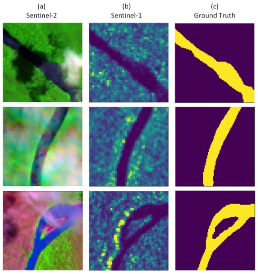
Figure 2.
Example of sample visualization and manual ground truth in the large-scale multi-source river imagery dataset: (a) false color composite image of Sentinel-2 satellite data; (b) false color composite image of Sentinel-1 satellite data; (c) manually-created ground truth (yellow color indicates water extent).
2.2. Proposed Method
We propose a contrastive learning process to extract representative hidden features from multi-spectral data and SAR data. These hidden features are extracted by the proposed deep learning models and contain the common information between the multi-source data and the self-information of each type of the data. Here, we first describe the idea of contrastive learning used in our proposed method.
Let , and represent three samples within a dataset. Here, serves as an anchor sample and we consider the relationship between and to be relevant, and to be irrelevant. For example, can be a multi-spectral image patch from a specific region and can be a SAR image patch from the same region while is a SAR image patch from a different region. The goal of contrastive learning is to learn an embedding that achieves higher score for the relevant pair and lower score for the irrelevant pair [24], which is shown as follows:
where the function can be any similarity measure between two feature embeddings. Here, we hypothesize that data in different modalities (e.g., SAR and multi-spectral images) both contain key patterns that describe our detection target (i.e., water extent). The idea behind contrastive learning is to better extract such relevant information that is shared between multi-source input samples.
In our problem, we further extend such standard contrastive learning approach to improve the detection to extract both the relevant information shared across different data sources and the self-information that is unique to each data source. The intuition is that we not only make use of common knowledge from multi-spectral and SAR data, but also leverage their supplementary strengths (e.g., land cover spectral characteristics by multi-spectral data and surface textures and elevations by SAR) to improve the river mapping. In particular, we use and to represent two different types of data as input for the river segmentation task. We use the relevant pair to represent multi-source data samples (i.e., image patches) of two different data types taken from the same geographical region. In the meantime, the irrelevant pair represents multi-source data samples of two different data types taken from different geographical regions. The proposed algorithm in this paper contains three steps: (1) multi-source data common information extraction, (2) multi-source data self-information extraction and (3) information fusion-based segmentation.
2.2.1. Common Information Extraction
We develop a neural network structure to extract common information from multi-source data input, as shown in Figure 3.
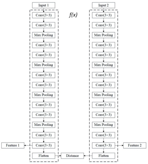
Figure 3.
The proposed common information extraction structure. Two dotted boxes represent the information extraction path f(x), as mentioned in Equation (1). During the training process, the goal of the model is to minimize the output of the ‘Distance’ layer with the same scene multi-source inputs. The ‘Feature1’ and ‘Feature2’ layers are blocked during the model training process and is used for further parameter transformation.
Here, we utilize the UNET staked convolutional and pooling layers in implementing the neural network structure of . The parameters in these neural network layers (used to compute ) can be trained based on the contrastive learning and will be further used for model testing.
During the training and testing process, we first train the proposed structure based on pseudo-code in Algorithm 1 and Algorithm 2. Algorithm 1 shows the pseudo-code for the model training. Here, we set up the training set with two different types of the sample pairs which are marked with a flag variable. Here, the flag variables are manually obtained during the multi-source sample pairs creation for common information extraction model training. the training sample pair with flag = 1 represents the relevant pair (ai,bi) and the training sample pair with represents the irrelevant pair (ai,bj). Given two input samples (e.g., ) and (e.g., or ), the loss function for extracting common information is defined as follows:
When flag = 0, the loss is computed as follows:
| Algorithm 1. Training process of the common information extraction structure |
| Input: Multi-source training sample pairs (SAR and multi-spectral data), flag (represents a multi-source training sample pair belongs to relevant or irrelevant type) |
| Output: Distance |
| 1: Block the ‘Feature1’ and ‘Feature2’ layers during the training process. |
| 2: Enable the ‘Distance’ layer during the training process. |
| 3: Set the ‘Input 1’ as the SAR sample input, the ‘Input 2’ as the multi-spectral sample input. |
| 4: for each multi-source training sample pairs do |
| 5: Fine-tuning the network parameters using loss function Loss (Input1, Input2, flag) defined in Equation (2). |
| 6: end for |
The m parameter is a constant, where . The m is the expected minimum distance between and . Here, Distance represents the distance between embeddings of and Imput2 and its value can be calculated using the Euclidean distance, as follows:
It can be observed that and Distance are negatively correlated, as shown in Equation (3). Thus, the goal of is to maximize the Distance between irrelevant pairs. Here, m denotes a threshold for distance penalty, i.e., we do not penalize an irrelevant pair (, bj) if the distance of between them is greater or equal to .
When flag = 1, the loss is calculated as follows:
It can be observed that and Distance are positively correlated, as shown in Equation (5). Thus, the goal of is to minimize the Distance between relevant pair . Thus, during the model training process, the model loss can be simplified into or based on the vector flag of current input training sample and could implement by the tensorflow platform.
Furthermore, Algorithm 2 shows the pseudo-code for the model testing. During the testing process, the multi-sources testing samples are set as the input of the structure and the common information matrices of the multi-sources testing samples are extracted from the ‘Feature 1′ and ‘Feature’ layers and will be further used in the information fusion process as described in Section 2.2.3.
| Algorithm 2. Testing process of the common information extraction structure |
| Input: Multi-source testing sample pairs (SAR and multi-spectral data) |
| Output: Common information at ‘Feature 1’ and ‘Feature 2’ layers |
| 1: Enable the ‘Feature1’ and ‘Feature2’ layers during the testing process. |
| 2: Block the ‘Distance’ layer during the testing process. |
| 3: Set the ‘Input 1’ as the SAR sample input, the ‘Input 2’ as the multi-spectral sample input. |
| 4: for each multi-source testing sample pairs do |
| 5: Achieve the common information matrices for multi-source testing sample pair from the ‘Feature1’ and ‘Feature2’ layers, separately. |
| 6: end for |
2.2.2. Self-Information Extraction
We also build a self-information extraction structure for each type of input data (i.e., multi-spectral data or SAR data). Our model architecture is inspired by the multi-scale feature extraction structure in UNET. As shown in Figure 4, the model is trained in a supervised way using data from each single source as input to predict the segmentation ground truth. We maintain two self-information extraction structures and have them trained separately using two types of input data. In this way, the hidden representation obtained from this extraction structure (e.g., the hidden layer before the final convolutional layers) can encode discriminative information about water extent using each single-source data.
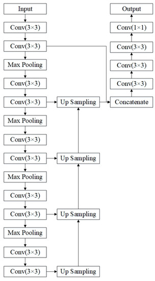
Figure 4.
The proposed self-information extraction structure. The self-information of the input data is captured by a multi-stage feature extraction structure and further generates the output using fused multi-stage feature and convolutional layers.
2.2.3. Information Fusion
In order to combine the extracted common information and self-information from the multi-source data inputs and perform the river segmentation task, we build an information fusion structure. We show the overall structure in Figure 5, which contains three paths. Firstly, the common information path extracts the common information from the multi-source data input. Secondly, the self-information path extracts the self-information from each type of the data within the multi-source data. Thirdly, the information fusion path concatenates the common information and self-information, then generates the final segmentation result.
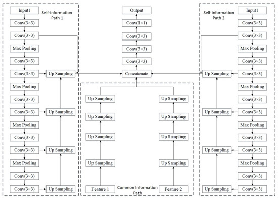
Figure 5.
The proposed information fusion based multi-source data segmentation structure. The proposed structure contains two self-information extraction path and a common information extraction path. The weights of these paths are copied from well-trained the common information extraction structure and self-information extraction structure, as mentioned in Figure 3 and Figure 4.
During the training process, the common information path and the self-information path are trained separately. Then, the parameters of the common information path and the self-information path are copied from the well-trained common information extraction model and self-information extraction model to initialize respective components in the overall model structure. Finally, the entire model will be trained using two types of inputs and training labels in a supervised fashion. The Binary Cross Entropy Loss is used for supervised training. Assuming we have training samples and we use and y to represent predicted labels and manually annotated labels, respectively, the loss function is defined as follows:
3. Results and Discussion
3.1. Experiment Setup
The experiment is conducted with Window 10, Python 2.7 and GTX2080 hardware environment. We also compare with several baseline segmentation methods including a popular water index-based approach, traditional machine learning approaches and state-of-the-art deep learning approaches.
Here, we setup several baselines in both single-source input style model and multi-source input style model. In order to achieve the multi-source input style model, we combine the SAR data (the sample size is 96 × 96 × 1) and multi-spectral data (the sample size is 96 × 96 × 9), which finally becomes a multi-source style input (the sample size is 96 × 96 × 10). These baselines include:
- NDWI: Normalized Difference Water Index is widely used to map water extent. We compute NDWI from multi-spectral imagery and threshold the obtained values of different pixels to obtain the river map.
- SVM and RF: Support Vector Machine and Random Forest are popular machine learning methods that have been widely used in remote sensing. Here, SVM-S2 and RF-S2 train the SVM and RF model using only Sentinel-2 data (SAR data) as input, separately. SVM-M and RF-M utilize the multi-source input as the model input during the model training and model testing.
- UNET: UNet is a popular deep learning model for pixel-wise classification (or segmentation) and was originally designed for medical image segmentation. Here, we setup three baseline methods, including UNET-S1, UNET-S2, UNET-M. UNET-S1 train the UNET model using only Sentinel-1 data (SAR data) as input. UNET-S2 train the UNET model using only Sentinel-2 data (SAR data) as input. UNET-M utilize the multi-source input as the model input during the model training and model testing.
- Non-contrastive: In order to verify the contribution of the common information during the segmentation process, we design the non-contrastive baseline as a variant of the proposed method by removing the common information path in the proposed structure. Here, the non-contrastive method utilized the multi-scale idea of the UNET and further setup a convolutional path starting with the concatenate layer, which could fusion the information from two self-information extraction path.
- We implement two versions of the proposed algorithm:
- Proposed Method A: The self-information extraction path and common information extraction path both utilize same amount of training samples (for which we have training labels) during the training process.
- Proposed Method B: The self-information extraction path is trained using labeled training samples. The common information extraction path utilizes all the samples (both labeled and unlabeled) since it can be trained in an unsupervised fashion. Finally, the information fusion part is trained using only the labeled data.
- The key hyper-parameters for the baselines and proposed method are shown in Table 3. The Contrastive Loss in Table 3 are described in Section 2.2.1.
Table 3. Parameters for the baselines and proposed method.
3.2. Large-Scale River Mapping
We divide the entire dataset (1013 samples) by randomly selecting 60% samples as the training set and the remaining 40% samples as the testing set. Then, we train the proposed method and baselines using the training set and validate these methods on the testing set. Here, the VV bands of the Sentinel-1 and the nine 10/20-m spatial resolution bands of the Sentinel-2 data are used for training and testing process.
Figure 6 and Figure 7 show the training curve for the proposed method. Firstly, we describe the ordinate and abscissa including model accuracy, model loss and epoch. The epoch represents the number of times that the model goes through the entire training dataset. The model accuracy is calculated based on the consistency between the model prediction and ground truth within a single epoch. The model loss represents the current loss value within a single epoch. As shown in Figure 6 and Figure 7, the accuracy and the loss reach the plateau after 30–40 epochs, which demonstrates that the model can be efficiently trained to achieve the convergence.
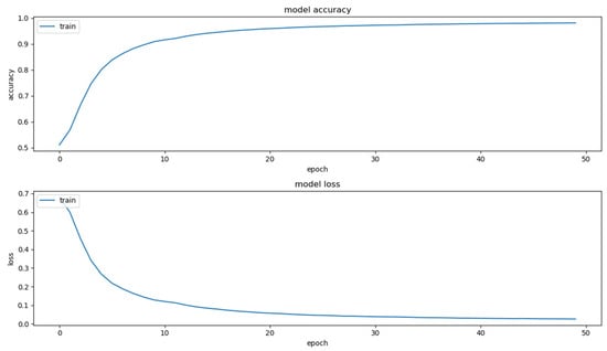
Figure 6.
The training curve of the proposed self-information extraction model.
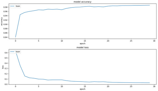
Figure 7.
The training curve of the proposed information fusion based multi-source data segmentation model.
Then, we evaluate the performance by measuring the F1-score, precision and recall among different methods, by using the 10m spatial resolution ground truth mask. Here, we briefly introduce the definition of these measures. Let TP represents the number of pixels that have been correctly predicted among river pixels. FP represents the number of pixels that have not been correctly predicted among river pixels. TN represents the number of pixels that have been correctly predicted among land pixels. represents the number of pixels that have not been correctly predicted among land pixels.
The precision is calculated by Equation (7):
The recall is calculated by Equation (8):
After gathering the precision and recall values, the F1-score is calculated by Equation (9). The F1-score is one of the widely used measuring methods and could convey the balance between the precision and the recall.
The comparison between the proposed method and baseline methods segmentation performance on the testing dataset is shown in Table 4. It can be observed that threshold-based NDWI method produces low F1-score for the large-scale river mapping task, due to the uncertainty in the reflectance spectral characteristics among different surface regions. Hence, we may need to use different thresholds for rivers in different places. The pixel-based machine learning method SVM and RF shows better performance on F1-score, compared with NDWI method. UNET-S1 method can better segment the river based on the concept of the receptive field idea, compared with SVM, RF and NDWI. Due to the improved spatial resolution of Sentinel-2 data, UNET-S2 method shows better segmentation result, compared with UNET-S1. Furthermore, the non-contrastive method outperforms other baselines on the F1-score. Overall, the proposed method shows best segmentation performance than other baselines. By comparing the proposed method A and the Non-contrastive method, we confirm the effectiveness of incorporating the common information extracted through contrastive learning in the final segmentation process. Furthermore, the Proposed Method B slightly outperforms the Proposed Method A, which demonstrates that the unsupervised common information model training process using more unlabeled data could better help the river segmentation process.
Table 4.
Comparison between the proposed method and baseline methods segmentation performance on the testing dataset.
We further visualize the segmentation results among the proposed method and baselines, using noise samples and limit samples. Figure 8 shows examples of river mapping results made by the proposed method and other state-of-the-art methods on large-scale river segmentation using noise samples. Each sample is first visualized by the Sentinel-1. Sentinel-2 and manually annotated ground truth, based on the proposed large-scale multi-source river imagery dataset, as mentioned in Section 2.1. As shown in Figure 8, the aerosol and cloud affect the river segmentation result among the threshold based NDWI method and the pixel-based machine learning methods. Here, we compare the single-source input style machine learning method RF-S2, SVM-S2 with multi-source input style machine learning model RF-M, SVM-M.
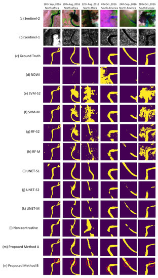
Figure 8.
The performance of the proposed method and other state-of-the-art methods on large-scale river segmentation, using noise image with cloud and aerosol. (a) test sample’s false color composite image based on Sentinel-2 satellite data; (b) test sample’s false color composite image based on Sentinel-1 satellite data; (c) test sample’s ground truth; (d) normalized difference water index(NDWI); (e) single-source input style support vector machine based on Sentinel-2 (SVM-S2); (f) multi-source input style support vector machine based on Senitnel-1 and Sentinel-2 (SVM-M); (g) single-source input style random forest based on Sentinel-2 (RF-S2); (h) multi-source input style random forest based on Senitnel-1 and Sentinel-2 (RF-M); (i) single-source input style UNET based on Sentinel-1 (UNET-S1); (j) single-source input style UNET based on Sentinel-2 (UNET-S2); (k) multi-source input style UNET based on Senitnel-1 and Sentinel-2 (UNET-M); (l) non-contrastive method is designed to show the performance of the proposed method without the common information path, by blocking the common information path in the proposed structure; (m) proposed method A; (n) proposed method B. Each column represents a random selected testing sample from the testing dataset. The red circle in each subfigure of the last row, represents the significate segmentation result improvement of the proposed method, while comparing with other state-of-the-art methods.
It can be seen that simply combine the multi-source data as the input could not help too much in the segmentation performance. UNET-S1 shows that the SAR data is able to better handle the fog and cloud and thus could obtain good river shape. However, due to the low resolution of the SAR data, the boundary of the segmentation result still need to be improved. In addition, the SAR data only has one channel, which makes it challenging for distinguishing the river content with many other different land covers. In addition, the proposed method B shows better river segmentation performance, especially within the noise part of the satellite image, compared with the baseline deep learning method UNET-S1, UNET-S2 and UNET-M. Additionally, Proposed Method A and Proposed Method B outperform the Non-contrastive method, which confirms the contribution of the common information extracted by the contrastive learning concept. The red circle within column (n) represents the significate improvement of the proposed method B, compared with other baseline methods. The result demonstrates the proposed method B is able to achieve better segmentation for large-scale surface area river mapping by using both labeled and unlabeled information.
3.3. River Mapping with Limited Labels
In practice, we may not have sufficient training samples if we want to map rivers in a specific year. Hence, we further evaluate the performance of our method and other existing methods on large-scale river segmentation using 20/100/200/400 training samples from the entire training set and present the F1-score performance among different methods in Table 5.
Table 5.
F1-Score Comparison between the proposed method and baseline methods segmentation performance on the testing dataset using different amount of training samples.
It can be seen that Multi-source input model Non-contrastive better segments the river under limited training sample condition, compared with single source input model UNET-S1 and UNET-S2. Furthermore, since the labeled data is often limited among many real world cases, the Proposed Method B is able to utilized the unlabeled data through offline training. Thus, the Proposed Method B performs better than the Proposed Method A due to the additional information from the unlabeled training samples, especially under limited labeled training sample conditions.
In addition, we show an example of detected river extent in Figure 9. It can be observed that the proposed method B shows better segmentation result among rest comparison methods.
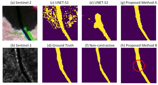
Figure 9.
The performance of the proposed method and other state-of-the-art methods on large-scale river segmentation with 400 training samples. (a) test sample’s false color composite image based on Sentinel-2 satellite data; (b) test sample’s false color composite image based on Sentinel-1 satellite data; (c) UNET for Sentinel-1; (d) test sample’s ground truth; (e) UNET for Sentinel-2; (f) non-contrastive method is designed to show the performance of the proposed method without the common information path, by blocking the common information path in the proposed structure; (g) proposed method A; (h) proposed method B. The red circle in (h) represents the significate segmentation result improvement of the proposed method B, while comparing with other state-of-the-art methods.
We further explore the method performance under different cloud coverage percentage condition. Figure 10 shows the segmentation accuracy curves using different cloud coverage samples. It can be observed that cloud coverage could highly influence the segmentation performance among all methods, due to the missing information in the foggy and cloudy satellite images. In addition, multi-source input model Non-contrastive outperforms several single-source input models, such as NDWI, SVM, RF and UNET-S1 and UNET-S2. Moreover, the Proposed Method B shows better segmentation F1-score than the Proposed Method A due to its ability to leverage unlabeled information during the unsupervised common information path training process.
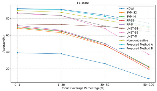
Figure 10.
The performance of the proposed method and other state-of-the-art methods on large-scale river segmentation under different cloud coverage percentage condition.
3.4. Long-Term River Monitoring
Finally, we can apply our proposed method for long-term river mapping, which can be very useful for monitoring and managing water resources. Figure 11 shows an example of the river monitoring over a two-year period. Figure 12 shows the river area estimation based on the water pixels from the river segmentation results. We can observe that the river regularly changes from season to season. In addition, it can be seen that the November’s river area from 2015 to 2017 shows an increasing trend.

Figure 11.
Long-term river monitoring Visualization based on river segmentation results. (a) Sentinel-2; (b) River Segmentation Result. Each column represents the river monitoring result among different time.
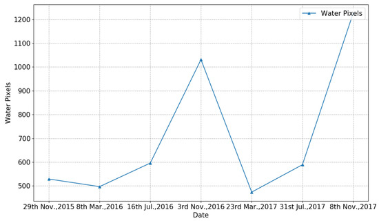
Figure 12.
Long-term river monitoring curve based on river segmentation results. The curve shows the amount of river pixels within the satellite imagery among different time.
4. Conclusions
In this paper we present a large-scale river mapping deep learning model based on contrastive learning and multi-source satellite data. We also create a large-scale multi-source river imagery dataset, along with handmade accurate river ground truth masks. The experiments show that the proposed method outperforms the several state-of-the-art segmentation methods and demonstrate that the proposed contrastive learning method is able to better segment the river over large spatial regions. Moreover, the proposed method shows better performance when multi-spectral satellite images are noisy (e.g., blocked by clouds).
In the future work, we plan to further validate our method using other types of high-resolution satellite data for longer term river monitoring and integrate these data sources in our dataset. Moreover, since there could be existed pixel error within current version of the proposed dataset when both optical and SAR images contain artifacts, we plan to refine the labels by utilizing an independent satellite data source (such as DigitalGlobe or WorldView). We will also study and extract temporal changes of water area in rivers, in order to automatically detect river expansion or shrinkage.
Author Contributions
Research conceptualization and methodology, Z.W., X.J.; research resources and data curation, Z.W., K.J., P.L.; writing—original draft preparation, Z.W.; writing—review and editing, Z.W., K.J., X.J., P.L., Y.X., Z.J.; supervision, K.J. All authors have read and agreed to the published version of the manuscript.
Funding
This research was funded by the Beijing Natural Science Foundation, grant number 4172001 and KZ201610005007 and Basic Research Program of Qinghai Province, grant number 2020-ZJ-709 and 2021-ZJ-704.
Institutional Review Board Statement
Not applicable.
Informed Consent Statement
Not applicable.
Data Availability Statement
Data sharing not applicable.
Conflicts of Interest
The authors declare no conflict of interest.
References
- Pekel, J.F.; Cottam, A.; Gorelick, N.; Belward, A.S. High-resolution mapping of global surface water and its long-term changes. Nature 2016, 540, 418–422. [Google Scholar] [CrossRef] [PubMed]
- Tarpanelli, A.; Iodice, F.; Brocca, L.; Restano, M.; Benveniste, J. River flow monitoring by sentinel-3 OLCI and MODIS: Comparison and combination. Remote Sens. 2020, 12, 3867. [Google Scholar] [CrossRef]
- Ogilvie, A.; Poussin, J.C.; Bader, J.C.; Bayo, F.; Bodian, A.; Dacosta, H.; Dia, D.; Diop, L.; Martin, D.; Sambou, S. Combining Multi-Sensor Satellite Imagery to Improve Long-Term Monitoring of Temporary Surface Water Bodies in the Senegal River Floodplain. Remote Sens. 2020, 12, 3157. [Google Scholar] [CrossRef]
- Kutser, T.; Pierson, D.C.; Kallio, K.Y.; Reinart, A.; Sobek, S. Mapping lake CDOM by satellite remote sensing. Remote Sens. Environ. 2005, 94, 535–540. [Google Scholar] [CrossRef]
- McFeeters, S.K. The use of normalized difference water index (NDWI) in the delineation of open water features. Int. J. Remote Sens. 1996, 17, 1425–1432. [Google Scholar] [CrossRef]
- Xu, H.Q. A study on information extraction of water body with the modified normalized difference water index (MNDWI). J. Remote Sens. 2005, 9, 589–595. [Google Scholar]
- Liu, Q.; Huang, C.; Shi, Z.; Zhang, S. Probabilistic River Water Mapping from Landsat-8 Using the Support Vector Machine Method. Remote Sens. 2020, 12, 1374. [Google Scholar] [CrossRef]
- Pal, M. Random forest classifier for remote sensing classification. Int. J. Remote Sens. 2005, 26, 217–222. [Google Scholar] [CrossRef]
- Ronneberger, O.; Fischer, P.; Brox, T. U-net: Convolutional networks for biomedical image segmentation. In International Conference on Medical Image Computing and Computer-Assisted Intervention; Springer: Cham, Germany, 2015; pp. 234–241. [Google Scholar]
- Zhao, H.; Shi, J.; Qi, X.; Wang, X.; Jia, J. Pyramid scene parsing network. In Proceedings of the IEEE Conference on Computer Vision and Pattern Recognition, Honolulu, HI, USA, 21–26 July 2017; pp. 2881–2890. [Google Scholar]
- Maxwell, A.E.; Warner, T.A.; Fang, F. Implementation of machine-learning classification in remote sensing: An applied review. Int. J. Remote Sens. 2018, 39, 2784–2817. [Google Scholar] [CrossRef] [Green Version]
- Lary, D.J.; Alavi, A.H.; Gandomi, A.H.; Walker, A.L. Machine learning in geosciences and remote sensing. Geosci. Front 2016, 7, 3–10. [Google Scholar] [CrossRef] [Green Version]
- Mou, L.; Bruzzone, L.; Zhu, X.X. Learning spectral-spatial-temporal features via a recurrent convolutional neural network for change detection in multispectral imagery. IEEE Trans. Geosci. Remote Sens. 2018, 57, 924–935. [Google Scholar] [CrossRef] [Green Version]
- Zhang, X.; Zhang, Y.; Lu, X.; Bai, L.; Chen, L.; Tao, J.; Wang, Z.; Zhu, L. Estimation of Lower-Stratosphere-to-Troposphere Ozone Profile Using Long Short-Term Memory (LSTM). Remote Sens. 2021, 13, 1374. [Google Scholar] [CrossRef]
- Mueller, N.; Lewis, A.; Roberts, D.; Ring, S.; Melrose, R.; Sixsmith, J.; Lymburner, L.; Mclntyre, A.; Tan, P.; Curnow, S.; et al. Water observations from space: Mapping surface water from 25 years of Landsat imagery across Australia. Remote Sens. Environ. 2016, 174, 341–352. [Google Scholar] [CrossRef] [Green Version]
- Tanguy, M.; Chokmani, K.; Bernier, M.; Poulin, J.; Raymond, S. River flood mapping in urban areas combining Radarsat-2 data and flood return period data. Remote Sens. Environ. 2017, 198, 442–459. [Google Scholar] [CrossRef] [Green Version]
- Zhu, Z.; Wang, S.; Woodcock, C.E. Improvement and expansion of the Fmask algorithm: Cloud, cloud shadow, and snow detection for Landsats 4–7, 8, and Sentinel 2 images. Remote Sens. Environ. 2015, 159, 269–277. [Google Scholar] [CrossRef]
- Immerzeel, W.W.; Droogers, P.; De Jong, S.M.; Bierkens, M.F.P. Large-scale monitoring of snow cover and runoff simulation in Himalayan river basins using remote sensing. Remote Sens. Environ. 2009, 113, 40–49. [Google Scholar] [CrossRef]
- Wei, Z.; Jia, K.; Jia, X.; Khandelwal, A.; Kumar, V. Global River Monitoring Using Semantic Fusion Networks. Water 2020, 12, 2258. [Google Scholar] [CrossRef]
- Xie, Y.; Shekhar, S.; Li, Y. Statistically-Robust Clustering Techniques for Mapping Spatial Hotspots: A Survey. arXiv 2021, arXiv:2103.12019. [Google Scholar]
- Jia, X.; Khandelwal, A.; Mulla, D.J.; Pardey, P.G.; Kumar, V. Bringing automated, remote-sensed, machine learning methods to monitoring crop landscapes at scale. Agric. Econ. 2019, 50, 41–50. [Google Scholar] [CrossRef]
- Arking, A.; Childs, J.D. Retrieval of cloud cover parameters from multispectral satellite images. J. Appl. Meteorol. Clim. 1975, 24, 322–333. [Google Scholar] [CrossRef] [Green Version]
- Dai, P.; Ji, S.; Zhang, Y. Gated Convolutional Networks for Cloud Removal From Bi-Temporal Remote Sensing Images. Remote Sens. 2020, 12, 3427. [Google Scholar] [CrossRef]
- Chen, T.; Kornblith, S.; Norouzi, M.; Hinton, G. A simple framework for contrastive learning of visual representations. In International Conference on Machine Learning; PMLR: Cambridge, MA, USA, 2020; pp. 1597–1607. [Google Scholar]
Publisher’s Note: MDPI stays neutral with regard to jurisdictional claims in published maps and institutional affiliations. |
© 2021 by the authors. Licensee MDPI, Basel, Switzerland. This article is an open access article distributed under the terms and conditions of the Creative Commons Attribution (CC BY) license (https://creativecommons.org/licenses/by/4.0/).