Abstract
In permafrost regions, active layer thickness (ALT) observations measure the effects of climate change and predict hydrologic and elemental cycling. Often, ALT is measured through direct ground-based measurements. Recently, synthetic aperture radar (SAR) measurements from airborne platforms have emerged as a method for observing seasonal thaw subsidence, soil moisture, and ALT in permafrost regions. This study validates airborne SAR-derived ALT estimates in three regions of Alaska, USA using calibrated ground penetrating radar (GPR) geophysical data. The remotely sensed ALT estimates matched the field observations within uncertainty for 79% of locations. The average uncertainty for the GPR-derived ALT validation dataset was 0.14 m while the average uncertainty for the SAR-derived ALT in pixels coincident with GPR data was 0.19 m. In the region near Utqiaġvik, the remotely sensed ALT appeared slightly larger than field observations while in the Yukon-Kuskokwim Delta region, the remotely sensed ALT appeared slightly smaller than field observations. In the northern foothills of the Brooks Range, near Toolik Lake, there was minimal bias between the field data and remotely sensed estimates. These findings suggest that airborne SAR-derived ALT estimates compare well with in situ probing and GPR, making SAR an effective tool to monitor permafrost measurements.
1. Introduction
Warming of the Arctic is leading to intensification of hydrologic cycles, changes to vegetation, increased river discharge, and elevated permafrost temperatures [1]. The permafrost active layer—the near-surface portion of the soil column that thaws annually in the summer—is at the nexus of change in the terrestrial Arctic system because it is a key zone for lateral groundwater flow, hosts ecological communities, and serves as the upper boundary of the permafrost [2]. Multi-scale quantification of the maximum depth that suprapermafrost soil thaws annually—the active layer thickness (ALT), primarily controlled by the maximum temperature achieved at a given location during the summer—serves as a robust indicator of climate change impacts on the Arctic [3], at many scales across Arctic landscapes. Furthermore, the high spatial heterogeneity of ALT [4] is a motivation to map ALT at high spatial resolution. This has inspired the development of a variety of tools, based on remote sensing datasets or statistical relationships, to map ALT.
The Circumpolar Active Layer Monitoring (CALM) network has acquired ALT data since the 1990s at over 200 sites in both hemispheres on 1 km2 or 1 ha grids using direct manual push probe measurements [5]. However, the locations of CALM sites are biased towards accessible places, and there is a need to estimate ALT across the vast remote expanses of the Arctic. Other efforts have focused on making more spatially extensive maps of ALT. Statistically and physically driven models have been used to produce catchment and regional ALT maps [6,7]. Others have used statistical correlations in conjunction with regional scale measurements to map ALT [8]. Recent approaches based entirely on remote sensing measurements have shown that satellite Interferometric Synthetic Aperture Radar (InSAR) data can be used to generate maps of ALT based on the seasonal subsidence of the land surface due to freeze-thaw cycles in the active layer [9]. Alternative SAR-based methods have used backscatter signals to estimate ALT [10,11].
Recently, the possibility has arisen of using aircraft-mounted SAR systems to acquire datasets for ALT estimation similar to what had previously been observed using satellites [12]. Although airborne SAR deployments have the disadvantage that they are not placed into Earth orbit, whereas satellites in orbit for long durations can repeat temporal measurements up to every 12 days in the Arctic [13]. On the other hand, aircraft deployments have the positive characteristic that they can be tasked to meet specific time-over-target objectives, and aircraft-mounted sensors can often achieve finer ground resolution than spaceborne SAR platforms. Furthermore, aircraft missions are far less costly than satellite missions and indeed may be more cost efficient on a per-square-meter basis than field surveys for measuring ALT on the catchment- or regional-scales. In 2017, as a part of NASA’s Arctic-Boreal Vulnerability Experiment (ABoVE) project, an airborne SAR dataset was acquired using the L-band Uninhabited Aerial Vehicle Synthetic Aperture Radar (UAVSAR) over Alaska and Western Canada with measurements collected in spring (April to June) and fall (September to November). The objective of ABoVE was to reveal environmental changes over large scales in the Arctic and boreal regions of North America. The airborne campaign included collection of UAVSAR data and P-band Airborne Microwave Observatory of Subcanopy and Subsurface (AirMOSS) polarimetric synthetic aperture radar (PolSAR) on 66 total flight lines covering >4 million km2 [14].
Our purpose is to validate airborne SAR-derived ALT measurements using calibrated field geophysical data. We also present a limited comparison between remotely sensed soil volumetric water content (VWC) estimates and VWC measured in the field. Specifically, our objective is to show quantitative statistical validation of these remotely sensed products in three characteristically different permafrost regions of Alaska. This validation demonstrates the ability of the remotely sensed ALT measurements to match field-based observations within uncertainty, enabling end users to have confidence in the utility of the airborne SAR ALT product. We use probe-calibrated ground penetrating radar (GPR) data as a well-established ground truth measurement of thaw depth that can efficiently acquire data on km-scales needed to validate the remote sensing results. While the maximum seasonal thaw, i.e., ALT, is not achieved until September or October each year, there is only a slight additional downward advancement of the thaw front between late August and October [11,15], and therefore, we treat GPR- and probe-measured thaw depth as a proxy for ALT.
2. Materials and Methods
The Permafrost Dynamics Observatory (PDO) data product [16] estimates seasonal subsidence, ALT, soil moisture, and uncertainties at 30-m resolution for 66 airborne flight lines across the ABoVE domain [17] in Alaska and northwest Canada. Throughout the rest of the text, we refer to the SAR-derived ALT product as “the PDO product”. The PDO retrieval uses L-band Synthetic Aperture Radar (SAR) data acquired by UAVSAR and P-band SAR backscatter acquired by AirMOSS. As part of the ABoVE airborne campaign, NASA flew all 66 lines in June and again in August 2017 [14]. The PDO product estimates seasonal subsidence due to thawing of the active layer using InSAR of the two L-band images acquired in June and August 2017. The PDO product estimates the vertical profile of soil volumetric water content (VWC) from the seasonal subsidence and the P-band backscatter from the August flights.
We focus on three SAR swaths in Alaska across a latitudinal gradient for this validation: Utqiaġvik/Barrow (BRW), Toolik (TOO), and the Yukon–Kuskokwim Delta (YKD) (Figure 1). The abbreviations indicated in parentheses are consistent with naming schemes used in the SAR dataset (i.e., barrow, toolik, and ykdelt) [16]. The BRW swath includes a lowland coastal plain underlain by continuous permafrost and has a mean annual air temperature (MAAT) of −11 °C and <200 mm of precipitation. The TOO swath includes the rolling topography of the foothills of the Brooks Range underlain by continuous permafrost and a MAAT of −7 °C and <400 mm precipitation. The YKD swath includes delta plain lowlands underlain by discontinuous permafrost and a MAAT of −1 °C and <480 mm of precipitation. The surface environmental conditions at all swaths are similar, being dominated by moss, lichen, and forbs, and sporadic shrubs adjacent to surface water. The mechanical probing and GPR validation datasets described below for BRW and TOO are described by [18,19].
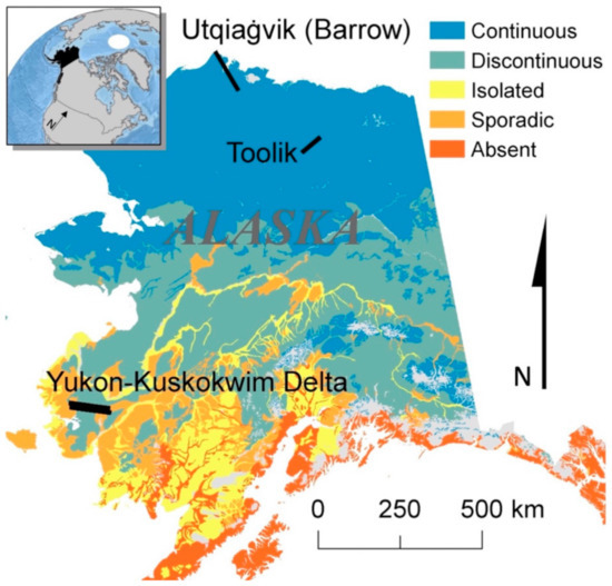
Figure 1.
Airborne SAR swaths (black patches) and the permafrost classification across Alaska, USA [20].
ALT was measured using GPR calibrated to mechanical thaw probe observations. Thaw probing was done using a 1.5 m long, graduated steel rod that was inserted vertically into the active layer until refusal at the ice-bonded permafrost table, following the CALM protocol. The operator judged if the contact was permafrost or rock based on the feeling and sound of the impact. Depending on the site, thaw probe measurements were made sporadically (e.g., >100 m between probe locations) along the GPR transect to capture the large-scale spatial variability in ALT and soil characteristics; however, in some cases, high-density transects of probing at 1 m intervals were also measured to capture small-scale variability. Repeatability—the measurement of mechanical probing uncertainty—was measured occasionally by measuring in triplicate within a 0.3 m diameter circle.
All GPR data used for validation were measured using the instrumentation, settings, and protocol described by [19] with a Malå ProEx (GuidelineGeo, Stockholm, Sweden). Data were processed using ReflexW (Sandmeier Geophysical Research, Karlsruhe, Germany). The GPR transmits a radio-frequency electromagnetic (EM) pulse at a 500 MHz center frequency that propagates downward into the ground. At the permafrost table, where there is a contrast in dielectric permittivity between frozen and unfrozen materials, the EM wave is reflected back towards the instrument, and the total travel time of the wave is recorded as a waveform or ‘trace’. The resulting radargram images composed of many adjacent traces are processed to remove low frequency noise and enhance late-time arrivals before being manually interpreted to extract—or ‘pick’—the GPS-tagged reflection arrivals. The GPR data was acquired in ‘tracks’ of semi-continuous measurements automatically triggered every 0.3 s at walking speed resulting in a total of 1.9 × 10⁵ data points across all swaths (Figure 2). The approximate spatial measurement footprint is 0.3 m2, based on the material properties and distance to the permafrost table. If the velocity is known, travel time can be converted to ALT. Probe measurements of ALT co-located with GPR observations of travel time allow for calculation of velocity. We calculated a velocity for each co-located probe and GPR measurement within a swath and then used the average velocity for that swath to perform the time-depth-conversion for all other points in that swath. Uncertainty on ALT observations derived from GPR was estimated using the standard deviation of GPR velocity (σv) for each swath, i.e., supposing σv = 0.006 m ns−1, that would correspond to ALT uncertainty of 0.065 m for a 0.5 m ALT. GPR data were measured 10–15 August 2013 for the BRW swath, 11–14 August 2014 for the TOO swath, and 13–16 August 2016 for the YKD swath. At locations where collocated GPR and thaw probe measurements were available, the calculated velocity was converted to depth-integrated VWC using an empirical equation calibrated for permafrost soils in AK [21]. We employed the depth-integrated VWC because the GPR is sensitive to the total water content throughout the active layer depth profile, in comparison to conventional soil moisture probes, e.g., time-domain reflectometry (TDR), that is limited to measurement over the length of the probe’s waveguides (10 to 20 cm).
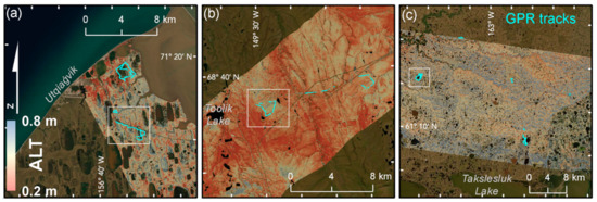
Figure 2.
Ground penetrating radar (GPR) tracks displayed over the PDO product for the (a) BRW, (b) TOO, and (c) YKD swaths. The locations of these swaths are indicated in Figure 1. White boxes indicate locations shown in Figure 9. Latitude and longitude tick marks are in 5’ intervals. Dark patches within the terrestrial landscape are water bodies.
Airborne SAR data were collected using UAVSAR and AirMOSS radars, with two flights acquired along each swath during 2017: one near the onset of thaw, and another towards the end of the thaw season. The subsidence estimated across each swath between the L-band UAVSAR acquisitions is used to estimate ALT based on the principle that the ground surface subsides when the water in the soil melts, resulting in a decrease in the pore water volume [9]. The P-band AirMOSS backscatter is sensitive to soil dielectric properties down to ~60 cm depth. The PDO product uses both L-band InSAR and P-band backscatter to estimate seasonal subsidence, ALT, and soil volumetric water content product at 30 m pixel resolution. By estimating the water content, and assuming a typical subsurface porosity profile, the required ALT to produce the measured subsidence is calculated in a joint inversion framework [12]. Given that the SAR acquisitions are not precisely at the beginning and end of the thaw period, an accumulated degree days of thaw (ADDT) correction is applied to extrapolate the total seasonal subsidence (and therefore ALT) from the measured subsidence, based on the ADDT experienced at each swath. Full details of the postprocessing and joint retrieval can be found in [12]. The ALT product is masked to eliminate pixels with heavy forest cover and InSAR coherence < 0.35 [12].
Given the approximate two orders of magnitude scale difference between the footprint of the GPR and SAR pixel size, we averaged the GPR data in each PDO pixel. We used the same 30 m grid that the SAR results are presented on [17] and calculated the mean, standard deviation, and count of the GPR data within each pixel. Uncertainty on the averaged pixels is estimated using Gaussian error propagation where the GPR measurement error described above is added in quadrature to the scaling error (standard deviation of GPR measurements in each pixel), and representation error accounting for the difference in time between the SAR acquisition and the fieldwork, estimated as 0.045 m based on the average observed interannual variability at all three swaths (https://www2.gwu.edu/~calm/, accessed on 25 June 2021). Given the tortuous path of the GPR track across the landscape, some pixels have hundreds of ALT measurements, while others may have fewer than ten (the median count was 74 GPR points per 30 m × 30 m pixel across all sites). To ensure a representative ALT value for each validation pixel, we rejected any pixels that had fewer than 30 ALT measurements, following the Central Limit Theorem. Once the GPR dataset is calibrated for local wave velocity, upscaled to a 30 m grid, and reduced to eliminate pixels with low data count, we refer to the final product as the ‘ALT validation dataset’. As detailed in [18], we use the χ2 statistic that accounts for observational uncertainty to compare the remotely sensed product to the validation dataset. χ2 at each pixel is calculated as:
where rn is the residual between the PDO product and ALT validation dataset at pixel n, and ε0,n is the uncertainty in the validation dataset at pixel n. Ideal matches occur if both estimated values are within the uncertainty of each other. This means the difference between the remotely sensed and GPR ALT is smaller than uncertainty, implying the two are statistically identical. Good matches occur if the estimated ground measured value is only within the uncertainty of the SAR measurement, a marginal match is when only the uncertainties overlap, and all others are classified as ‘no match’. The overall χ2 is calculated as:
where N is the total number of pixels where ALT is observed.
3. Results
3.1. Calibrated GPR Dataset
Here, we focus on the dataset measured within the YKD swath as a representative example. This dataset was referred to by [22]; however, the details are first reported here. The calibrated GPR datasets measured within the BRW and TOO swaths are detailed in [19,23], respectively, and therefore we direct the reader to those publications for comprehensive explanations of those datasets. The example processed radargram (Figure 3a) shows the undulating, semi-discontinuous reflection from the permafrost table. The GPR pulse reflects at any boundary with a dielectric contrast, such as the thawed-frozen boundary at the bottom of the active layer. This is a typical image where the reflection is clearly visible along most of the line, though there are intermittent segments where no obvious reflection is present (e.g., near trace 1450) perhaps due to poor coupling or variations in the dielectric permittivity contrast [19]. Above the permafrost table reflection, there are moderately continuous to discontinuous subparallel reflections. The earliest time reflections < 10 ns may be associated with an interface between peat and mineral soil. The more horizontal arrivals above the permafrost table may also be associated with instrument noise or antenna ringing. Figure 3b shows a comparison between the probe data and GPR data after calibration to the local average wave velocity, where probe uncertainties are calculated as the standard deviation of three replicate probe measurements at the same location. A perfect match between the probe and GPR data would fall exactly along a one-to-one line, and deviation of points from the one-to-one line is primarily a result of spatial variability in soil moisture that is not accounted for when using a site-wide velocity. The average site-wide velocities for all swaths are shown in Table 1.
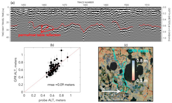
Figure 3.
GPR results from within the YKD swath. (a) Processed radargram with time-depth-conversion applied using site-calibrated wave velocity. The interpreted reflection from the permafrost table is indicated in red. (b) Comparison between GPR-measured ALT and thaw probe data with one-to-one line. (c) Location where the radargram in (a) was measured (white arrow), also showing the SAR ALT product overlain on aerial imagery. The GPR track is shown in the southeast corner of Figure 2c.

Table 1.
Average () and standard deviation (σ) for the SAR and validation (VAL) datasets and for the GPR wave velocity, v.
3.2. Comparison of Validation Dataset to Airborne SAR
A direct comparison of the validation dataset with the PDO product (Figure 4a) shows BRW to have the thinnest active layer, TOO intermediate, and YKD as thickest. The TOO result falls approximately around the one-to-one line, while the BRW results indicate that the SAR product slightly overestimates ALT on average, while at YKD the SAR result slightly underestimates ALT on average. Despite these small biases, the error bars on the average SAR results do overlap the one-to-one line. Visualizing the same data as a 2D histogram (Figure 4b) illustrates that the relationship is somewhat linear when considering the more frequent occurrence of points close to the one-to-one line. The overall root mean squared error (RMSE) between the PDO product and validation dataset is 0.176 m, which translates to 20–70% ALT uncertainty.
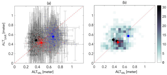
Figure 4.
(a) ALT validation data compared against the collocated SAR result. Grey bars are individual estimated uncertainties (vertical error bars indicate posterior uncertainty for the PDO product; horizontal error bars indicate validation uncertainty from error propagation of the GPR errors, scaling errors, and representation errors); large colored markers are the average and standard deviations for each swath. (b) A 2D histogram, where grayscale indicates count, displaying the same data as in panel (a). Black, BRW; red, TOO; blue, YKD.
3.3. Validation Results Based on Airborne SAR Coherence
Including only the highest quality pixels in the validation reduces the RMSE (Figure 5). In Figure 4, we used all SAR pixels above the coherence threshold of 0.35. The magnitude of the correlation is referred to as the “coherence” [24]. As coherence increases, the uncertainty in the estimated ALT decreases, making it more difficult to reach the ideal match criteria in the χ2 statistic. Nevertheless, the higher quality pixels with high coherence show reduced RMSE. Setting a higher coherence threshold reduces the number of pixels in the validation statistics. For example, if we set the coherence threshold to 0.65, the RMSE decreases to 0.09 m, 0.16 m, and 0.17 m for TOO, BRW, and YKD respectively, while reducing the number of usable pixels in the validation statistics to about 300. Depending on the application, a user of the PDO dataset could define their own coherence threshold to focus on the highest quality pixels with the lowest uncertainties, at the cost of fewer usable pixels per swath and less spatially continuous data coverage.
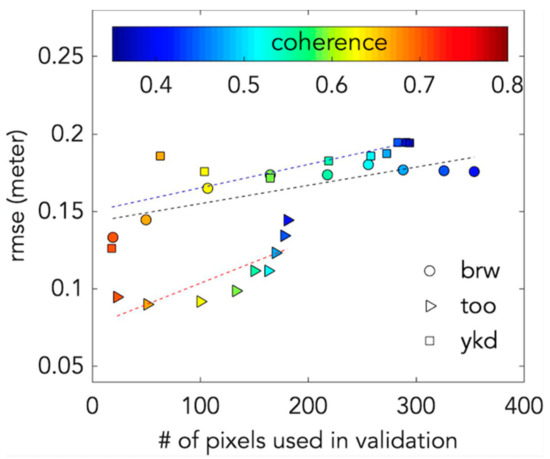
Figure 5.
The relationship between the number of pixels used for validation and the resulting RMSE, showing that when SAR pixels are culled by coherence, a smaller RMSE can be achieved at the expense of a smaller statistical population.
These results indicate that noise in the data influences the accuracy of the results, as opposed to a problem with the retrieval. Coherence loss is driven by noise in the interferogram, which in turn results from small differences in surface scattering between the two scenes. The pixels with the least amount of noise tend to converge towards the validation data, resulting in lower RMSE.
3.4. Uncertainty Assessment
Here we address the uncertainty of each measurement method. For probing measurements, the only site where we have estimates of measurement repeatability is YKD. Given that these distributions appear to be skewed (Figure 6), particularly the SAR, we report the median rather than the mean. The probe measurements have the lowest uncertainty, likely because the primary sources of error are simply the operators’ judgment of the ground surface and the ability to read the 0.01 m graduations marked on the probe. The scaled GPR data has around double the uncertainty of the probe data, due to both velocity uncertainty and scaling. SAR uncertainty is two to three times larger than GPR due to errors both in the measurement (as a result of having infrequent acquisitions from airborne platforms), as well as assumptions in the conversion from subsidence to ALT. Please refer to [12] for more details on SAR uncertainties.
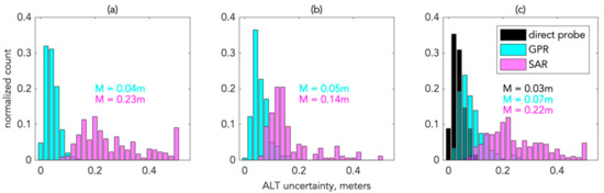
Figure 6.
Frequency distributions of ALT uncertainty for the (a) BRW, (b) TOO, and (c) YKD swaths. Median values (M) are reported for each frequency distribution.
3.5. Evaluation of ALT Observations across Measurement Methods
Next, we illustrate a comparison of the ALT frequency distributions of each measurement for each swath. Histograms indicate the SAR and GPR data are visually similar, though statistically different (Figure 7). Although we do not expect the populations to have equivalent distributions or even to exhibit Gaussian shape, we nonetheless tested this possibility statistically using the nonparametric Kruskal–Wallis test [25]. This non-parametric one-way analysis of variance (ANOVA) test on ranks compares whether all four populations originate from the same distribution. Resulting p-values > 0.05 would indicate that they are not significantly different, however we found that the p-values were <0.05 in all cases: pBRW = <10−6, pTOO = 0.0025, pYKD = <10−6. This mismatch is attributed to the contrasting sampling area of each measurement: ~0.01 m2 for probing, ~0.3 m2 for GPR and 900 m2 for SAR that each have the capacity to detect variability in ALT on different spatial scales. At BRW (Figure 7a) there are notable shifts in the peaks of the histograms between the total GPR dataset and the 30 m scaled validation GPR dataset. Although this may seem counterintuitive given that both were derived from the same population, this difference arises because many of the GPR points were not included in the scaled validation product due to either failing to meet the 30 point-per-pixel threshold or because the GPR measurement was in a location that was masked out of the SAR swath due to low SAR coherence. In contrast, the frequency distributions for each measurement population with the TOO and YKD swaths are approximately coincident.
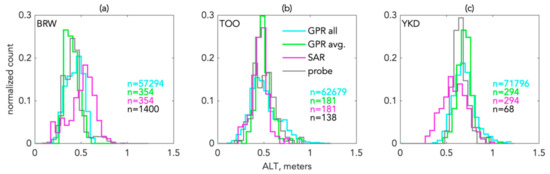
Figure 7.
Histograms of ALT for the (a) BRW, (b) TOO, and (c) YKD swaths.
3.6. Volumetric Water Content Comparison
While our primary focus is the validation of ALT estimates, here we provide a basic comparison of VWC estimates from the joint retrieval against field measurements. We are restricted to a limited comparison for VWC because our field measurements only observe depth-integrated VWC when there are collocated probe and GPR measurements, and this only occurs sporadically every few hundred meters along each GPR track. Therefore, a single depth-integrated VWC observation that may not be representative of the local average conditions would be compared to a 30 m SAR pixel. Furthermore, at BRW where there are more probe data available, they are distributed across only 11 pixels, which is too few to make a statistical argument. The histograms at BRW (Figure 8a) are different from the SAR-estimated values substantially underestimating field measurements. Comparison of the VWC histograms at TOO and YKD (Figure 8b,c) reveals that the populations are similar with median differences of 0.03 m3 m−3 and 0.08 m3 m−3 respectively, suggesting a close match between SAR-derived VWC and field conditions.
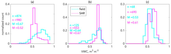
Figure 8.
Frequency distributions of VWC for the (a) BRW, (b) TOO, and (c) YKD swaths. Population counts, n, indicate the total number of individual depth-integrated VWC observations and the number of pixels for the field and SAR datasets respectively. M indicates median.
3.7. χ2 Classification Results
The χ2 classification quantifies how well SAR pixels match the field data within uncertainty. These results are summarized in Table 2 for all observations and grouped by swath. The positive bias at BRW indicates SAR overestimated ALT, while the negative biases at the other swaths indicate SAR underestimated ALT. In total, 79% of all pixels were either an ideal match or a good match with the validation dataset—ideal matches being statistically identical. TOO had the highest percentage of good match or better (82%), while YKD had the smallest percentage in those categories (77%).
Table 2.
Results of χ2 classification. RMSE indicated root mean squared error, nSAR is the number of SAR pixels available for validation.
To illustrate how the χ2 classified pixels are distributed across the landscape, we present pixels along representative GPR tracks from each swath in Figure 9a–c. The tracks do not appear spatially continuous for two reasons: (1) we rejected SAR pixels with less than 30 validation ALT measurements, and (2) SAR pixels with coherence less than 0.35 are not used in the validation. Residuals are plotted spatially in Figure 9d–f. There are no obvious spatial patterns in either the classifications or the residuals (i.e., spatial patterns χ2 are approximately random), except that the residuals appear to be more positive in BRW and more negative in YKD, corresponding to the overall observed bias (Table 2). The approximate randomness of χ2 spatial patterns suggests that cases of marginal match or no march likely result from random noise than a systematic bias or problems with the PDO retrieval.
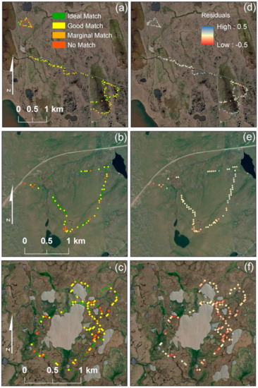
Figure 9.
χ2 classifications for (a) BRW, (b) TOO, and (c) YKD with corresponding residuals (d–f).
4. Discussion
4.1. Evaluation of Validation Data
ALT may vary substantially even over short distances on the scale of meters (e.g., Figure 3a). Using the minimum threshold of 30 GPR-measurements-per-pixel produces a statistically representative ALT observation for each pixel, corresponding to a data density of 3 measurements per 100 m2. The median point density across all of our sites is 8 measurements per 100 m2, and the maximum is 54 measurements per 100 m2. For comparison, the data density at a 1 km2 CALM grid is around 0.01 measurement per 100 m2.
We found the median uncertainty on the direct manual thaw probe measurements in the YKD swath to be 0.03 m (Figure 7c) based on triplicate measurements within a 0.3 m radius. This is equivalent to the 0.03 m uncertainty reported within the BRW swath [18], and similar to the 0.04 m uncertainty reported for sandy arctic soils [10]. Given this consistency in mechanical probe uncertainty, we judge this level of uncertainty to be appropriate to apply to probing data for all of our study areas.
The direct comparison of probe measurements to coincident calibrated GPR observations (Figure 3b) highlights the effectiveness of GPR for noninvasively measuring an interface between thawed and frozen soil. Similar comparisons have been made [18,19] illustrating the overall linearity of the relationship, but also some expected spread of the data away from the one-to-one line due to spatial variation in VWC. While the variation in VWC (i.e., proportional to permittivity or wave velocity) is clear from Figure 3b, across the datasets from all three sites, there is relatively low variation in the mean wave velocity (Table 1). This may be useful information for other studies that cannot perform detailed calibrations.
Obtaining coincident measurements in time remains a substantial challenge, particularly when coordinating aircraft and ground teams. The aircraft may acquire data across the whole state of Alaska in the time it takes the field team to acquire validation measurements at a single site. There are related restrictions when attempting to coordinate the measurement timing with natural processes such as the maximum depth of thaw corresponding with ALT. As described, it was impossible to acquire contemporaneous field validation datasets, and indeed our field measurements were in some cases years different from the aircraft flights. Based on available timeseries data, we accounted for this representation error to the best of our ability, however, we nonetheless acknowledge that ALT experiences interannual variability that cannot entirely be accounted for in our approach, which may have resulted in some false positives and false negatives in our χ2 classification.
While our field ALT measurements were made in August rather than the end of the thaw season in September or October, we assume these measurements approximate maximum thaw due to the deceleration of the thaw front late in the season. While we do not have detailed models or timeseries data exactly at our swaths, we consider previously presented modeling results [11,15] that modeled active layer thaw dynamics at 70°N latitude. The results of these studies indicated that between August 14 (approximately the time of measurement of our field data) and the onset of freezing, the permafrost table only advanced 0.01–0.03 m, which is within the uncertainty of both our probing and GPR data. Therefore, we judge the seasonal timing of our data collection to have a negligible effect on the validation results.
Although our VWC validation is limited due to the low data density of field measurements, we nonetheless highlight the importance of using depth-integrated VWC obtained from GPR observations. For typical soil moisture probes—e.g., TDR and similar dielectric approaches—the VWC is measured as an average along the length of the waveguides. While there is nothing physically incorrect about this, if a user is attempting to make minimally invasive observations (i.e., not digging a pit) by inserting the waveguides vertically into the ground surface this will only sample the top, partially saturated portion of the soil column. Such measurements are not representative of the soil water content throughout the active layer as demonstrated by the lack of correlation between depth-integrated VWC measurements and TDR probes [26]. In contrast, time-consuming soil pits disturb the tundra sufficiently to prevent future re-measurement, and soil pits likely influence the in situ soil moisture distribution. Furthermore, it is impractical to dig a large enough number of soil pits to achieve the spatial representativeness we seek herein.
4.2. Comparison of Large-Scale ALT Estimates
Two general approaches for making large scale maps of ALT are (1) remotely sensed observations of active layer properties and processes, or (2) discrete or indirect observations extended to large scales using spatial statistics. The first group is further divided into observations from either airborne or spaceborne sensor platforms. Given that satellites in orbit are continuously acquiring images at the same location on an approximately 12 day interval, ALT estimates from spaceborne SAR sensors have an advantage of long duration continuous deployment, meaning that ALT estimates may be derived from data measured multiple times per thaw season for several consecutive years [9]. In contrast, airborne platforms have the potential flexibility to target specific observation times and provide measurements at finer spatial resolution and possibly at multiple radar frequency bands.
Previously calculated satellite-based ALT estimates within the BRW swath were found to underestimate ALT by 0.02 m compared to field data [18], which is smaller than the 0.10 m overestimate in the PDO product we found using airborne measurements (Table 2) at similar pixel size. The difference in native spatial resolution (i.e., the intrinsic instrument resolution before spatial averaging) between airborne and spaceborne SAR could be responsible for this observed bias [12]. Furthermore, the spaceborne InSAR dataset was composed of many more SAR scenes than the airborne dataset [18]. The bias (0.10 m) observed in the airborne dataset is similar to the airborne-ALT uncertainty (+/−0.14 m), the validation dataset uncertainty (+/−0.07 m) (Table 1), and the spaceborne-ALT uncertainty (+/−0.19 m) [18]. The spaceborne-ALT results within the BRW swath were found to achieve a χ2 category of either ideal match or good match at 74% of validation pixels, similar to the 80% of pixels in the same category for the airborne-ALT measurement (Table 2). Within the YKD swath, previously calculated satellite-ALT observations revealed that 66% of pixels were either ideal or good matches [22], compared to 78% in the same categories for the airborne-ALT observations (Table 2).
An example of a large-scale ALT estimate made using spatial statistics is available in the Yukon Flats region [8]. This area is closest to the TOO swath, although the Yukon Flats region is on the border between continuous and discontinuous permafrost and has different geologic substrate and landscape history, so we do not intend to draw a direct comparison between these two sites. Nonetheless, we observe that statistically predicted ALT around Ft. Yukon had a bias of approximately −0.09 m for a 30 m × 30 m pixel size [8], similar to the bias of −0.04 m we observed at the TOO swath (Table 2). A different statistical ALT estimate approach of the 26,000 km2 Kuparuk River basin which partially includes the TOO swath found a bias of 0.02 m for estimates on a 300 m × 300 m pixel size, though the validation set was limited to 12 points scaled up from the 121-point CALM grids [6]. Even larger scale estimates of ALT have been attempted on the Russian Arctic drainage basin using climate inputs as drivers and assumptions about soil variables in a Stefan equation framework [7]; however, the extremely sparse direct observations make this scale of ALT product challenging to compare with our validation, though the modeled ALT is reported to be underestimated. SAR Backscatter-derived ALT estimates on the Yamal peninsula, Russia, achieved an RMSE of 0.2 m for ALT ranging from 0.8 to 1.4, or uncertainty of 14–25% [10].
4.3. Value and Limitations of Airborne SAR Estimates of ALT and VWC
There are several potential areas where airborne-SAR estimates of ALT may provide particular advantages compared to other large-scale ALT mapping methods. Perhaps most notable is the potential to retrieve subsurface VWC estimates concurrently with ALT due to the implications for developing a more complete understanding of hydrology and energy balance if both parameters are available [26]. Our present validation of VWC is limited, though it suggests promise for the accuracy of the VWC parameter (Figure 8). Currently, it is not possible to directly estimate VWC from spaceborne-ALT measurements for the whole active layer depth from spaceborne microwave instruments due to limited penetration depth, and existing spatial statistical models have not attempted to include this property directly. Another potential value of airborne-derived ALT estimates is the possibility of recovering finer-scale ALT variability. Although in this study we used 30 × 30 m pixels, this was a choice driven by the objective of using a standardized grid to enable different science datasets to be integrated and analyzed easily [17]. Using a different flight plan and a more frequent intra-seasonal measurement interval could allow for ALT and VWC retrieval at 10 m resolution.
One limitation of airborne-estimated ALT is that measurements can only be acquired when flights are tasked to do so. Therefore, SAR analysis may need to be conducted on fewer datasets than might be available from spaceborne platforms, resulting in the need to use spatial averaging and upscaling from the native resolution to achieve an acceptable signal-to-noise ratio in the SAR data. While 30 m pixel resolution may be acceptable when considering a swath that covers nearly 2500 km2, it is also important to recognize that ALT varies substantially on the meter-scale (Figure 3a).
Although our comparison is limited to three swaths, the data (Figure 4) may suggest that airborne SAR may overestimate ALT when the true value is thinner (northern latitude) and underestimate ALT when the true value is thicker (southern latitude). While the three swaths detailed herein do represent a wide range of latitude, a detailed examination of more swaths within the latitude gradient would help to reveal if this bias is limited to BRW, TOO, and YKD or if it is systematic and linked to some aspect of the data acquisition or processing [12]. Additionally, based on the field VWC measurements (Figure 8), soil moisture is greatest in BRW and least at YKD, raising the possibility that limitations in the ability to retrieve ALT VWC may be partially responsible for the bias in Figure 4. The surface characteristics of all sites are similar, with low typical tundra vegetation and no trees, and therefore we anticipate this is not a key factor in the bias shown in Figure 4.
4.4. Future Research on Validating Remotely Sensed Active Layer Products
GPR-derived ALT datasets [19,23] have been successfully demonstrated as a field survey technique for validating SAR-estimated ALT products [18,22] due to the capability of GPR to acquire tens of thousands of ALT data points in large scale transects at acceptable uncertainty levels. Here we have further bolstered confidence in this approach and added important details related to scaling such as a minimum validation point density threshold and propagation of scaling uncertainty to the validation product. Illuminating the linkages and correspondence between SAR, GPR, and probe-measured ALT and study sites features is a key future research task. There are additional refinements that could be made to improve future validations.
First, it would be valuable to have more spatially extensive VWC field data to validate the VWC component of the joint retrieval. This is particularly challenging because each point where VWC is estimated requires 1–2 min of measurement and recording time at a minimum to complete the direct probing. So-called ‘high-density’ transects of 100 m total length and 1 m spacing between VWC measurements have been explored [23] with the objective of capturing some of the fine-scale spatial variability in ALT and VWC. However, in the best case, one high-density transect only could be used to validate up to three 30 m SAR pixels. Although this approach would approximately meet our criteria of validating SAR pixels only if there are >30 field data points within the pixels, the high-density surveys are a large time investment for a limited amount of validation. It would be useful to explore the spatial correlation length scales for VWC that may help to justify tolerance of <30 field data points per pixel. Furthermore, soil pits would be useful for characterizing the porosity profile [11] to allow for saturation calculations, and improved site-specific dielectric-VWC transforms may enable higher precision VWC estimates. To that end, we also emphasize the importance of acquiring depth-integrated VWC measurements, either in addition to or instead of conventional soil moisture probe (waveguide) measurements because depth-integrated VWC has been demonstrated to have the strongest correlation with active layer physical processes [27].
Another area of work would be the extension of the continuous multi-offset GPR approach for measuring ALT [27]. This simultaneously retrieves velocity and travel time, thereby eliminating the need for probe measurements beyond quality assurance/quality control. This multi-offset approach would have the additional advantage of resolving the challenge of spatially sporadic VWC measurements described above. Past efforts at this approach have been limited to simple, flat surface microtopography due to complications that arise with GPR antenna positioning on rough surfaces, and distinct subsurface layering (e.g., peat over mineral soil). It is possible that coupling a multi-layer GPR inversion [28] with the multi-offset acquisition scheme and using a ridged antenna sled that slides across the tundra vegetation may help to overcome these limitations.
4.5. Implications for Monitoring Thaw, Mapping ALT and Model Parameterizations
Monitoring ALT is valuable for understanding how permafrost landscapes are changing in response to climate warming—currently, this is primarily achieved through the network of CALM sites [4]. While this network of sites is extremely valuable for permafrost monitoring, the 1 km2 manually-probed site scale cannot capture the dynamics of all landscape features. Therefore, the PDO product validated herein provides a useful baseline against which future observations may be compared. While it may not be possible to re-fly all swaths annually, a decadal resurvey of the measured swaths may reveal landscape-scale patchiness or other changes to ALT outside the resolution of the CALM grids.
Permafrost hydrology modeling relies on ALT because this is the primary zone for water dynamics—e.g., lateral flow—in continuous permafrost landscapes. Distributed hydrologic models use ALT as an input parameter that defines the depth to the impervious layer [29]. ALT is similarly important to permafrost carbon (C) modeling because this depth defines the boundary between bioavailable C and permafrost-sequestered C that may be released to the atmosphere under future warmer climate scenarios [30]. The validated PDO product is at an ideal scale for watershed hydrology or C cycling models—either as input parameters or to validate the results if ALT is calculated physically within the model [15,31].
5. Conclusions
We have demonstrated that 79% of the airborne-derived ALT values PDO product pixels are either an ideal match or good match χ2 classes in comparison with the field validation dataset. Overall, the RMSE between the PDO product and validation dataset is 0.176 m, which equates to a deviation in ALT between the two datasets of 20–70%. Considering the χ2 and RMSE results together, the airborne SAR-derived ALT products exhibit accuracies similar to previously-reported large-scale ALT estimation methods, and therefore we conclude that the airborne SAR-derived ALT products are successfully validated within uncertainty.
Author Contributions
Conceptualization, A.D.P. and K.S.; methodology, A.D.P., T.D.S., K.S., R.H.C., R.J.M.; formal analysis, A.D.P.; writing—original draft preparation, A.D.P.; writing—review and editing, K.S., R.H.C., R.J.M., T.D.S., L.K.C., L.H., Y.Z., E.W., M.M., H.Z.; project administration, K.S.; funding acquisition, K.S., M.M., H.Z., A.D.P. All authors have read and agreed to the published version of the manuscript.
Funding
This research was funded by NASA, grant numbers NNX13AM25G, NNX14A154G, NNX16AH36A, and NNX17AC59A.
Data Availability Statement
The data used in the manuscript are available at: https://doi.org/10.3334/ornldaac/1355, https://doi.org/10.3334/ORNLDAAC/1796, http://dx.doi.org/10.3334/ORNLDAAC/1265, and https://doi.org/10.3334/ORNLDAAC/1903 (all accessed on 25 June 2021).
Acknowledgments
We thank S. Schaefer, S. Ludwig, and S. Natali for assistance in the field acquiring data in the Yukon-Kuskokwim Delta. We thank the US Fish and Wildlife Service for permitting fieldwork in the Yukon-Kuskokwim Delta.
Conflicts of Interest
The authors declare no conflict of interest.
References
- Box, J.; Colgan, W.T.; Christensen, T.R.; Schmidt, N.M.; Lund, M.; Parmentier, F.-J.W.; Brown, R.; Bhatt, U.S.; Euskirchen, E.S.; Romanovsky, V.E.; et al. Key indicators of Arctic climate change: 1971–2017. Environ. Res. Lett. 2019, 14, 045010. [Google Scholar] [CrossRef]
- Hinzman, L.D.; Kane, D.L.; Gieck, R.E.; Everett, K.R. Hydrologic and thermal properties of the active layer in the Alas-kan Arctic. Cold Reg. Sci. Technol. 1991, 19, 95–110. [Google Scholar] [CrossRef]
- Van Everdinger, R. Multi-Language Glossary of Permafrost and Related Ground-Ice Terms (Revised 2005); National Snow and Ice Data Center/World Data Center for Glaciology: Boulder, CO, USA, 1998. [Google Scholar]
- Hinkel, K.M. Spatial and temporal patterns of active layer thickness at Circumpolar Active Layer Monitoring (CALM) sites in northern Alaska, 1995–2000. J. Geophys. Res. Space Phys. 2003, 108. [Google Scholar] [CrossRef]
- Abramov, A.; Davydov, S.; Ivashchenko, A.; Karelin, D.; Kholodov, A.; Kraev, G.; Lupachev, A.; Maslakov, A.; Ostroumov, V.; Rivkina, E.; et al. Two decades of active layer thickness monitoring in northeastern Asia. Polar Geogr. 2019, 1–17. [Google Scholar] [CrossRef]
- Nelson, F.E.; Shiklomanov, N.I.; Mueller, G.R.; Hinkel, K.M.; Walker, D.A.; Bockheim, J.G. Estimating Active-Layer Thickness over a Large Region: Kuparuk River Basin, Alaska, U.S.A. Arct. Alp. Res. 1997, 29, 367. [Google Scholar] [CrossRef]
- Zhang, T.; Frauenfeld, O.W.; Serreze, M.C.; Etringer, A.; Oelke, C.; McCreight, J.L.; Barry, R.; A Gilichinsky, D.; Yang, D.; Ye, H.; et al. Spatial and temporal variability in active layer thickness over the Russian Arctic drainage basin. J. Geophys. Res. Space Phys. 2005, 110, 1–14. [Google Scholar] [CrossRef]
- Pastick, N.J.; Jorgenson, M.T.; Wylie, B.K.; Minsley, B.J.; Ji, L.; Walvoord, M.A.; Smith, B.D.; Abraham, J.D.; Rose, J.R. Extending Airborne Electromagnetic Surveys for Regional Active Layer and Permafrost Mapping with Remote Sensing and Ancillary Data, Yukon Flats Ecoregion, Central Alaska. Permafr. Periglac. Process. 2013, 24, 184–199. [Google Scholar] [CrossRef] [Green Version]
- Liu, L.; Schaefer, K.; Zhang, T.; Wahr, J. Estimating 1992–2000 average active layer thickness on the Alaskan North Slope from remotely sensed surface subsidence. J. Geophys. Res. Space Phys. 2012, 117. [Google Scholar] [CrossRef]
- Widhalm, B.; Bartsch, A.; Leibman, M.; Khomutov, A. Active-layer thickness estimation from X-band SAR backscatter intensity. Cryosphere 2017, 11, 483–496. [Google Scholar] [CrossRef] [Green Version]
- Chen, R.H.; Tabatabaeenejad, A.; Moghaddam, M. Retrieval of Permafrost Active Layer Properties Using Time-Series P-Band Radar Observations. IEEE Trans. Geosci. Remote. Sens. 2019, 57, 6037–6054. [Google Scholar] [CrossRef]
- Michaelides, R.J.; Chen, R.H.; Zhao, Y.; Schaefer, K.; Parsekian, A.D.; Sullivan, T.; Moghaddam, M.; Zebker, H.A.; Liu, L.; Xu, X.; et al. Permafrost Dynamics Observatory (PDO)—Part I: Postprocessing and Calibration Methods of UAVSAR L-band InSAR Data for Seasonal Subsidence Estimation. Earth Space Sci. 2021. [Google Scholar] [CrossRef]
- Chen, J.; Günther, F.; Grosse, G.; Liu, L.; Lin, H. Sentinel-1 InSAR Measurements of Elevation Changes over Yedoma Uplands on Sobo-Sise Island, Lena Delta. Remote Sens. 2018, 10, 1152. [Google Scholar] [CrossRef] [Green Version]
- Miller, C.E.; Griffith, P.C.; Goetz, S.J.; Hoy, E.E.; Pinto, N.; McCubbin, I.B.; Thorpe, A.K.; Hofton, M.M.; Hodkinson, D.J.; Hansen, C.; et al. An overview of ABoVE airborne campaign data acquisitions and science opportunities. Environ. Res. Lett. 2019, 14, 080201. [Google Scholar] [CrossRef]
- Swenson, S.C.; Lawrence, D.; Lee, H. Improved simulation of the terrestrial hydrological cycle in permafrost regions by the Community Land Model. J. Adv. Model. Earth Syst. 2012, 4. [Google Scholar] [CrossRef]
- Schaefer, K.; Michaelides, R.J.; Chen, R.H.; Sullivan, T.D.; Parsekian, A.D.; Zhao, Y.; Bakian-Dogaheh, K.; Tabatabaeenejad, A.; Moghaddam, M.; Chen, J.; et al. ABoVE: Active Layer Thickness Derived from Airborne L-and P-band SAR, Alaska, 2017; ORNL DAAC: Oak Ridge, TN, USA, 2021. [Google Scholar] [CrossRef]
- Loboda, T.V.; Hoy, E.E.; Carroll, M.L. ABoVE: Study Domain and Standard Reference Grids, Version 2; ORNL DAAC: Oak Ridge, TN, USA, 2019. [Google Scholar] [CrossRef]
- Schaefer, K.; Liu, L.; Parsekian, A.; Jafarov, E.; Chen, A.; Zhang, T.; Gusmeroli, A.; Panda, S.; Zebker, H.A.; Schaefer, T. Remotely Sensed Active Layer Thickness (ReSALT) at Barrow, Alaska Using Interferometric Synthetic Aperture Radar. Remote Sens. 2015, 7, 3735–3759. [Google Scholar] [CrossRef] [Green Version]
- Chen, A.; Parsekian, A.D.; Schaefer, K.; Jafarov, E.; Panda, S.; Liu, L.; Zhang, T.; Zebker, H. Ground-penetrating ra-dar-derived measurements of active-layer thickness on the landscape scale with sparse calibration at Toolik and Happy Valley, Alaska. Geophysics 2016, 81, H9–H19. [Google Scholar] [CrossRef]
- Jorgenson, M.T.; Yoshikawa, K.; Kanevskiy, M.; Shur, Y.; Romanovsky, V.; Marchenko, S.; Grosse, G.; Brown, J.; Jones, B. Permafrost characteristics of Alaska. In Proceedings of the Ninth International Conference on Permafrost, University of Alaska, Fairbanks, AK, USA, 29 June–3 July 2008; Volume 3, pp. 121–122. [Google Scholar]
- Engstrom, R.; Hope, A.; Kwon, H.; Stow, D.; Zamolodchikov, D. Spatial distribution of near surface soil moisture and its relationship to microtopography in the Alaskan Arctic coastal plain. Hydrol. Res. 2005, 36, 219–234. [Google Scholar] [CrossRef]
- Michaelides, R.J.; Schaefer, K.; Zebker, H.A.; Parsekian, A.; Liu, L.; Chen, J.; Natali, S.M.; Ludwig, S.; Schaefer, S.R. Inference of the impact of wildfire on permafrost and active layer thickness in a discontinuous permafrost region using the remotely sensed active layer thickness (ReSALT) algorithm. Environ. Res. Lett. 2018, 14, 035007. [Google Scholar] [CrossRef]
- Jafarov, E.E.; Parsekian, A.D.; Schaefer, K.; Liu, L.; Chen, A.C.; Panda, S.K.; Zhang, T. Estimating active layer thickness and volumetric water content from ground penetrating radar measurements in Barrow, Alaska. Geosci. Data J. 2017, 4, 72–79. [Google Scholar] [CrossRef]
- Rosen, P.A.; Hensley, S.; Joughin, I.R.; Li, F.K.; Madsen, S.N.; Rodriguez, E.; Goldstein, R.M. Synthetic aperture radar interferometry. Proc. IEEE 2000, 88, 333–380. [Google Scholar] [CrossRef]
- Breslow, N. A generalized Kruskal-Wallis test for comparing K samples subject to unequal patterns of censorship. Biometrika 1970, 57, 579–594. [Google Scholar] [CrossRef]
- Clayton, L.K.; Schaefer, K.; Battaglia, M.J.; Bourgeau-Chavez, L.; Chen, J.; Chen, R.H.; Chen, A.; Bakian-Dogaheh, K.; Grelik, S.; Jafarov, E.; et al. Active layer thickness as a function of soil water content. Environ. Res. Lett. 2021, 16, 055028. [Google Scholar] [CrossRef]
- Gerhards, H.; Wollschläger, U.; Yu, Q.; Schiwek, P.; Pan, X.; Roth, K. Continuous and simultaneous measurement of reflector depth and average soil-water content with multichannel ground-penetrating radar. Geophysics 2008, 73, J15–J23. [Google Scholar] [CrossRef]
- Parsekian, A.D. Inverse Methods to Improve Accuracy of Water Content Estimates from Multi-offset GPR. J. Environ. Eng. Geophys. 2018, 23, 349–361. [Google Scholar] [CrossRef]
- Fabre, C.; Sauvage, S.; Tananaev, N.; Srinivasan, R.; Teisserenc, R.; Pérez, J.M.S. Using Modeling Tools to Better Understand Permafrost Hydrology. Water 2017, 9, 418. [Google Scholar] [CrossRef]
- Chaefer, K.; Zhang, T.; Bruhwiler, L.; Barrett, A.P. Amount and timing of permafrost carbon release in response to climate warming. Tellus B Chem. Phys. Meteorol. 2011, 63, 168–180. [Google Scholar] [CrossRef]
- Painter, S.L.; Coon, E.T.; Atchley, A.L.; Berndt, M.; Garimella, R.; Moulton, J.D.; Svyatskiy, D.; Wilson, C.J. Integrated surface/subsurface permafrost thermal hydrology: Model formulation and proof-of-concept simulations. Water Resour. Res. 2016, 52, 6062–6077. [Google Scholar] [CrossRef]
Publisher’s Note: MDPI stays neutral with regard to jurisdictional claims in published maps and institutional affiliations. |
© 2021 by the authors. Licensee MDPI, Basel, Switzerland. This article is an open access article distributed under the terms and conditions of the Creative Commons Attribution (CC BY) license (https://creativecommons.org/licenses/by/4.0/).