Article

Spatial, Phenological, and Inter-Annual Variations of Gross Primary Productivity in the Arctic from 2001 to 2019

1
College of Earth and Environmental Sciences, Lanzhou University, Lanzhou 730000, China
2
College of Geography and Environmental Sciences, Zhejiang Normal University, Jinhua 321004, China
3
Southern Marine Science and Engineering Guangdong Laboratory, Zhuhai 519000, China
4
University Corporation for Polar Research, Beijing 100875, China
*
Author to whom correspondence should be addressed.
Remote Sens. 2021, 13(15), 2875; https://doi.org/10.3390/rs13152875
Submission received: 26 May 2021 / Revised: 12 July 2021 / Accepted: 16 July 2021 / Published: 22 July 2021
(This article belongs to the Special Issue Remote Sensing of Land Surface Phenology)

Abstract

:
Quantifying the spatial, seasonal (phenological), and inter-annual variations of gross primary productivity (GPP) in the Arctic is critical for comprehending the terrestrial carbon cycle and its feedback to climate warming in this region. Here, we evaluated the accuracy of the MOD17A2H GPP product using the FLUXNET 2015 dataset in the Arctic, then explored the spatial patterns, seasonal variations, and interannual trends of GPP, and investigated the dependence of the spatiotemporal variations in GPP on land cover types, latitude, and elevation from 2001 to 2019. The results showed that MOD17A2H was consistent with in situ measurements (R = 0.8, RMSE = 1.26 g C m−2 d−1). The functional phenology was also captured by the MOD17A2H product (R = 0.62, RMSE = 9 days) in the Arctic. The spatial variation of the seasonal magnitude of GPP and its interannual trends is partly related to land cover types, peaking in forests and lowest in grasslands. The interannual trend of GPP decreased as the latitude and elevation increased, except for the latitude between 62°~66° N and elevation below 700 m. Our study not only revealed the variation of GPP in the Arctic but also helped to understand the carbon cycle over this region.

Graphical Abstract

1. Introduction

Climate change is causing permafrost melting [1], shrub cover expansion, growing season lengthening, and consequently, carbon flux changes in the Arctic [2]. Furthermore, the carbon cycle is also influenced by changes in vegetation phenology [3]. GPP, which is considered the biggest carbon flux of terrestrial ecosystems [4], not only plays a vital role in offsetting the concentration of greenhouse gases and mitigating global warming to a certain extent [5] but also builds a bridge between terrestrial and air carbon. In the context of the Arctic, the rate of climate warming is almost twice the global average, a phenomenon known as Arctic amplification [2,6,7,8,9,10]. Therefore, quantifying the spatial, seasonal (phenological), and inter-annual variations of Arctic GPP is critical for comprehending the carbon cycle and its feedback to climate warming.
Quantifying global or local GPP has received a great deal of attention in recent studies. Utilizing satellite-based near-infrared reflectance (NIRv) as the proxy of GPP and the revised light-use-efficiency model (i.e., EC-LUE model), Wang et al. [11] and Zheng et al. [12] explored the global spatial patterns of GPP with a spatial resolution of 0.05 degrees. However, the annual average estimates of GPP were not consistent during the same period. Wang et al. [11] reported a range of 128.3 ± 4.0 Pg C year−1 while Zheng et al. [12] reported a range of 106.2 ± 2.9 Pg C yr−1. Some studies have detected the GPP in the Arctic, but most paid attention to specific ecosystems (e.g., streams and moss communities) [13,14] and few efforts [12,15] have been devoted to investigating the specific situation of the Arctic GPP. Here, the MOD17A2H product was selected because it is one of the major official GPP products and has been most widely used in detecting the carbon cycle of terrestrial ecosystems [4,16]. Additionally, its finer resolution (500 m) can reveal detailed GPP variations in the Arctic.
Satellite products generally suffer from the uncertainty that results from complex data acquisition processes and limitations of retrieval algorithms. For this reason, different datasets lead to disparate results. MOD17 is based on the light-use-efficiency (LUE) concept, which is difficult to parameterize since it is influenced by land cover types, phenophases and different types of environmental stress. Furthermore, the maximal values of LUE are specified in the look-up tables for the same biota types, which might introduce uncertainties in GPP [17]. Although MOD17A2H, the v.6 product of MOD17, has overcome the limitation of the proposed year and filling method, the core issues caused by its algorithm still exist. In addition, MODIS (Moderate Resolution Imaging Spectroradiometer) products are inferred based on surface reflectance, which is only available when the relative accuracy of MODIS reflectance products can be determined [18]. Therefore, evaluating its performance is necessary before characterizing the spatiotemporal pattern of GPP. There have been many validation studies regarding the performance of MODIS GPP products at the global scale [19,20,21,22] and their accuracies over different biomes (e.g., grassland and forest) have been quantified [23]. However, the validation pixels belonging to specific biomes are often combined together and there are few specialized studies that quantify the accuracy of MOD17A2H in the Arctic. In fact, the performance of the MODIS GPP algorithm shows reasonable variations with climate regions and factors [18,19], species [24], and latitude [25]. Furthermore, the phenology (e.g., the peak timing of GPP) derived from satellite products is often mismatched in scale with in situ data [26]. Several studies have assessed the performance of phenological patterns of MOD17A2H in different regions or biomes [17,27]. However, it is unclear whether MOD17A2H is suitable for the Arctic. Therefore, there is a pressing need to investigate the accuracy of MOD17A2H in the Arctic.
The objective of this work was to utilize MOD17A2H to explore the spatial distribution and phenological characteristics of GPP in the Arctic. In particular, the goal was to (1) evaluate the performance of MOD17A2H in different conditions in the Arctic; (2) identify the spatial distribution and phenological characteristics of GPP, and detect the variation of GPP with land cover types, latitude, and elevation; and (3) detect the interannual trends of GPP in the Arctic and its relation with land cover types, latitude, and elevation. This article begins by describing the study area and the experimental data (Section 2). Section 3 explains the validation and trend detection methods. Section 4 provides the results and discussion of validation, spatial distribution, and phenological characteristics, as well as interannual trends of GPP. Finally, Section 5 presents a brief conclusion.

2. Study Area and Experimental Data
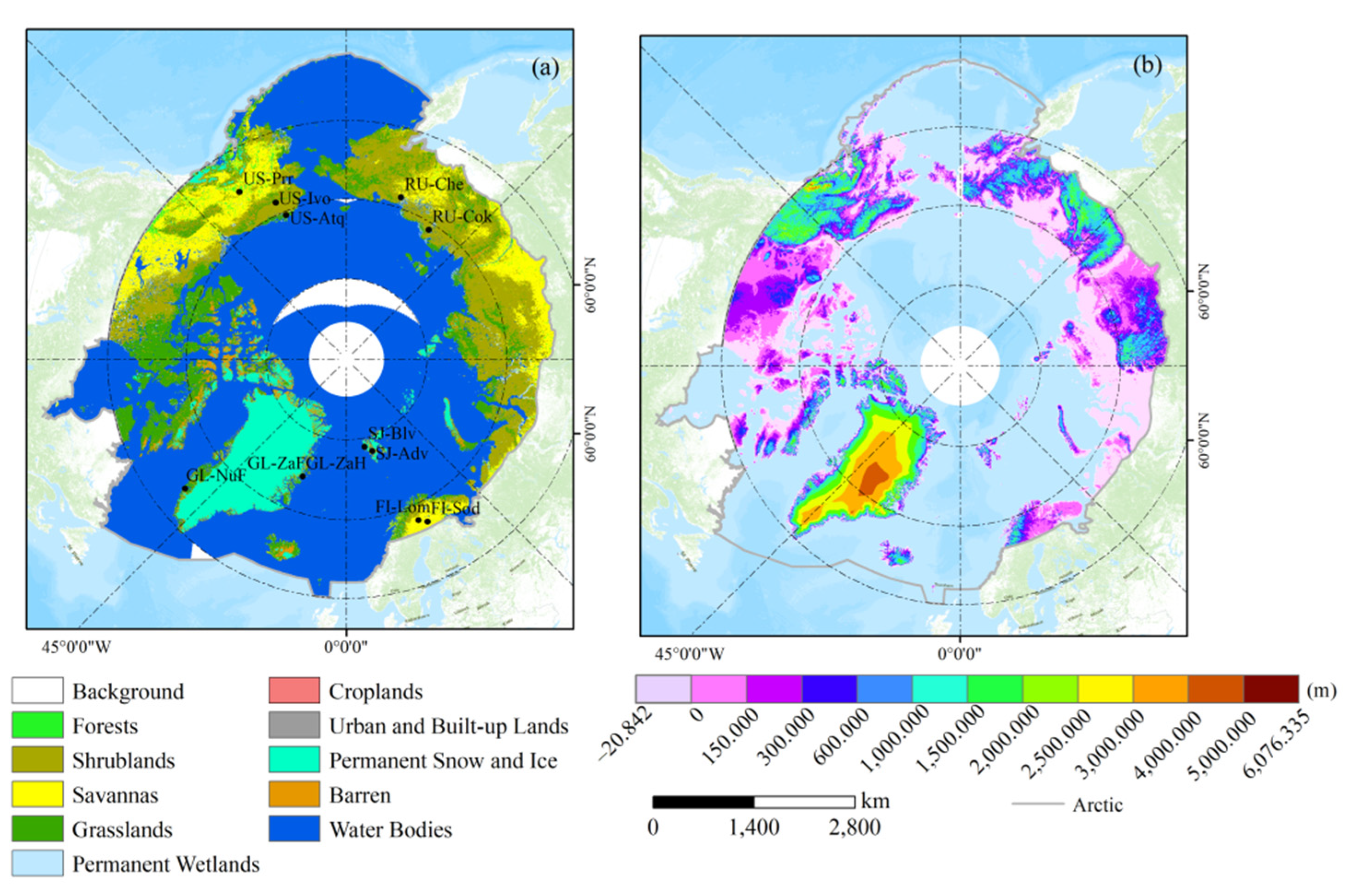
2.1. Study Area

The study region covers the area from 50° N to 90° N and is characterized by long cold winters and short summers. There is very little precipitation and the temperature is low. As a result of the harsh environments, there are few vegetation types in the Arctic. As shown in Figure 1a, water occupies more than half of the area in the Arctic, and the dominant vegetation type are shrubland (dominated by woody perennials), savannas (tree cover 10–60%), and grasslands (dominated by herbaceous annuals (<2 m)). Savannas are distributed in relatively low latitudes, while most of the shrublands are located at high latitudes. Grasslands are mainly scattered west of Greenland. The average altitude of the Arctic is below 1000 m. Areas with higher elevations are mainly distributed in the northwestern region of Canada, the northeastern region of Russia, as well as the Greenland Island and surrounding areas.

2.2. Data

2.2.1. FLUXNET Data

FLUXNET 2015 is the latest version of the FLUXNET dataset. Compared with previous datasets, FLUXNET v.2015 improves the protocols of data quality and the pipeline of data processing [28]. The Net Ecosystem Exchange (NEE) in the FLUXNET 2015 dataset was gap-filled with the marginal distribution sampling (MDS) method [29]. It was then partitioned into Ecosystem Respiration (RECO) and GPP using the daytime fluxes method (_DT) [30] and the nighttime fluxes method (_NT) [29]. The quality flags in FLUXNET 2015 are given values ranging from 0 to 1, indicating the percentage of high quality gap-filled and measured data [12]; 1 represents the highest quality and 0 represents the poorest quality [31].
As shown in Table 1, there are 12 sites in the FLUXNET datasets located in the study area, including 7 wetland sites, 2 forest sites, a grassland site, a shrublands site, and a permanent snow and ice site. This study used GPP (GPP_NT_VUT_REF) estimated from the night-time method with a daily temporal scale. The selection of GPP followed two criteria: (1) the quality flags were larger than 0.5; and (2) the difference between the GPP derived using the night-time method (GPP_NT_VUT_REF) and the day-time method (GPP_DT_VUT_REF) was lower than 50%. After filtering the data based on the two criteria, daily GPP were temporally aggregated to generate the 8-day averaged GPP, matching the temporal resolution of MOD17A2H.

2.2.2. Satellite Data

MOD17A2H (Collection 6) is a standard satellite product with a spatial resolution of 500 m and a temporal resolution of 8 days. It is calculated based on the light use efficiency (LUE) approach by Monteith [31]:
GPP   = ε   ×   fPAR   ×   PAR
where ε, fPAR, and PAR denote the radiation use efficiency coefficient (RUE), the fraction of incident PAR absorbed by the surface, and photosynthetically active radiation, respectively [32].
According to Running et al. [32], the GPP values of MOD17A2H refer to the sum of the GPP during an 8-day period. In this study, we averaged the total GPP to generate the 8-day averaged GPP.

2.2.3. Land Cover

The MCD12Q1 product provides global land cover type data at a spatial resolution of 500 m at an annual time step from 2001 to 2019. It is based on the supervised classification of MODIS reflectance data with six different classification schemes, including the IGBP (Annual International Geosphere-Biosphere Programmer), which was widely utilized due to its high accuracy and widespread acceptance [33]. Thus, the IGBP classification method was utilized in this study. The land cover data from 2001 to 2019 were chosen to produce a spatially continuous dataset via mosaic. The filling data of MCD12Q1 was removed to reduce their effect on the results. Evergreen needleleaf forests, evergreen broadleaf forests, deciduous needleleaf forests, deciduous broadleaf forests, and mixed forests were grouped into forests. Closed shrublands and open shrublands were grouped together as shrublands. Woody savannas and savannas were combined into savannas.

2.2.4. DEM (Digital Elevation Model)
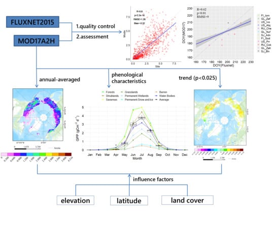
Multi-Error-Removed Improved-Terrain (MERIT) DEM is an improvement of SRTM3 (Shuttle Radar Topography Mission v.3) DEM, with a spatial resolution of 3 arc-second (~90 m). It removes multiple error components from the SRTM3 DEM, including stripe noise caused by the sensor error, speckle noise of surface reflectance, absolute bias derived from the limited control points of the ground, and tree height bias where the canopies were incorrectly classified as the land surface [34,35]. MERIT was chosen because its accuracy is higher than that of SRTM and NASADEM (NASA Digital Elevation Model) [36] and because of the data availability in the Arctic. In order to match the resolution of MOD17A2H, the DEM dataset was resampled to 500 m using the bilinear method.

3. Methods

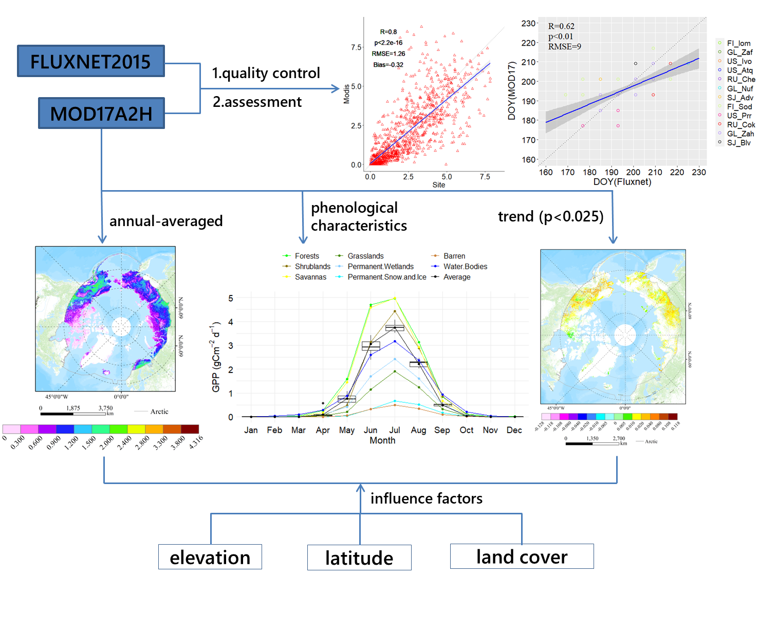
3.1. Accuracy Assessment

Although the validation based on in situ leaves issues of scale unresolved, which might introduce uncertainties to the verification, it is still an important method in regions lacking long-term validation data [37,38,39]. Here, the direct comparison method was utilized because it is simple and easy to implement. To avoid the influence of data noise, geometric mismatch, and spatial heterogeneity on the validation results, the average of the 3 × 3 pixels of MOD17A2H centered around tower coordinates in situ was used to match with in situ as suggested by Ueyama et al. [40].
Statistical indices, including the coefficient of correlation (R), root mean square error (RMSE), and Bias were used to indicate the accuracy of MOD17A2H [41]. R measures the consistency between MOD17A2H and in situ data, while RMSE measures the average absolute error of the MOD17A2H over a single in situ. Bias describes the average deviation between MOD17A2H and in situ measurements:
R = l = 1 h ( P l P ¯ ) ( O l O ¯ ) / l = 1 h ( P l P ¯ ) 2 l = 1 h ( O l O ¯ ) 2 ,
RMSE = l = 1 h ( P l O l ) 2 / h ,
Bias = l = 1 h ( P l O l ) / h
where P l and O l are the MOD17A2H and in situ-based GPP on the l th time period, respectively. P ¯ and O ¯ are the averaged value of the MOD17A2H and in situ-based GPP time series, respectively. h is the total number of time periods.
The assessment was twofold. First, the performances of the MOD17A2H product were assessed separately over each site. Second, by combining the data points of all sites within each specific land cover type, the accuracies of MOD17A2H over different land cover types were assessed and compared.

3.2. Comparison of Phenological Patterns between In Situ and MOD17A2H

The phenological patterns in ecosystem GPP are important in the terrestrial carbon cycle and have significant ecological implications. To understand if the MOD17A2H satellite GPP product can capture the functional phenology, which has been defined as the interaction and close association between plant functional traits and phenology [42], of in situ GPP, we first filled the data gap in the original 8-day GPP time series using a linear interpolation method. The gap-filled GPP time series was further smoothed using the Savitzky-Golay (SavGol) filter with a window size of 9 time steps and a second-order polynomial, which not only eliminated noise but also preserved the basic phenological attributes [43]. Finally, we extracted the timing of maximum GPP (day of year, DOY) during the photosynthetically active period for each site from both the in situ and MOD17A2H data. Agreement between the peak timings extracted from the in situ GPP and those extracted from the MOD17A2H was used as an indicator of the performance of the MOD17A2H GPP product in representing the functional phenology patterns of arctic ecosystems.

3.3. The Spatial Distribution Characteristics Identification and Trend Detection

The spatial distribution of GPP was explored. First, the pixel-wise multiyear averaged monthly GPP was calculated to check the GPP spatial distribution and the phenology patterns in different months. Second, the annual-maximum and annual-averaged GPP were identified to detect the distribution of GPP in the Arctic.
A pixel-based simple linear regression, in which time is the independent variable and GPP is the dependent variable, was applied to detect the trend of GPP. In addition, the significance of the interannual trend was evaluated utilizing the Mann–Kendall (MK) test [44], and the significant trends (p < 0.025) of the Arctic were retained.
In this study, both MOD17A2H data and the linear regression function were provided by Google Earth Engine (GEE), which is a cloud-based computing platform for planetary-scale data analysis, mapping, and modeling, providing free access to numerous global datasets and advanced computational capabilities [45]. GEE was employed for the following reasons: it provides easy access to the MOD17A2H datasets and other related datasets such as land cover types and elevation; it enables rapid exploration of long time series datasets without downloading them; and it provides a library of functions such as linear regression function, which are applied for data analysis and result display.

4. Results and Discussion

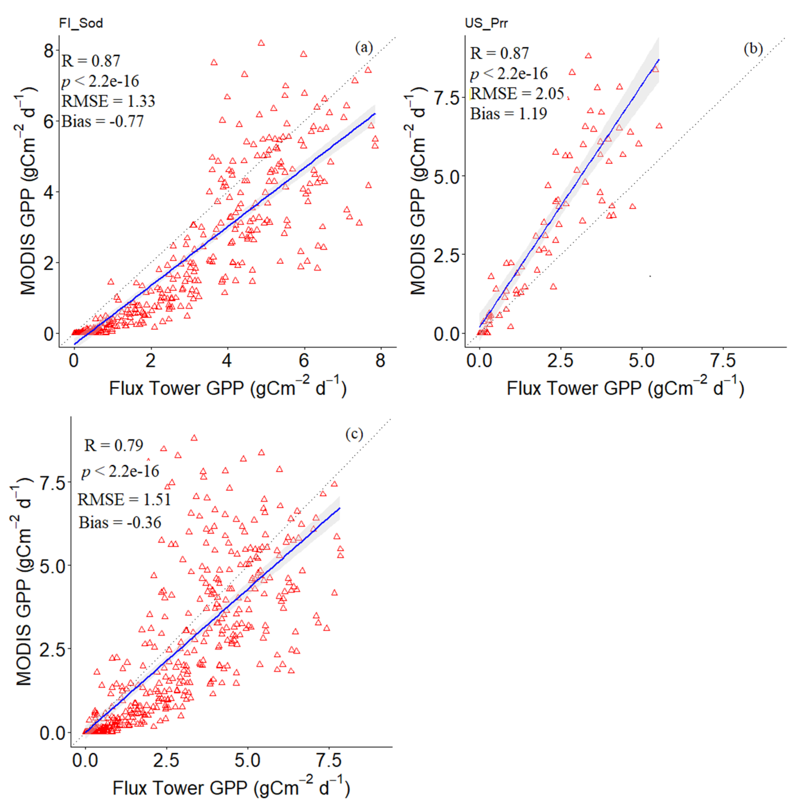
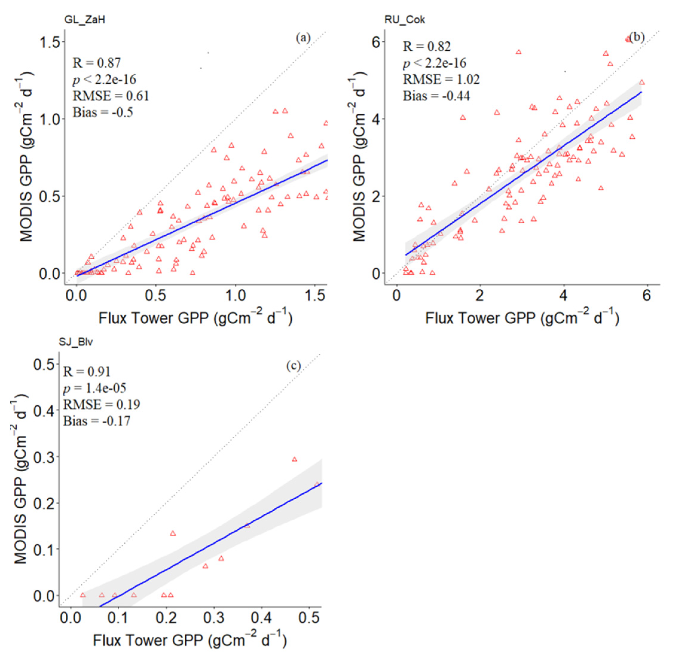
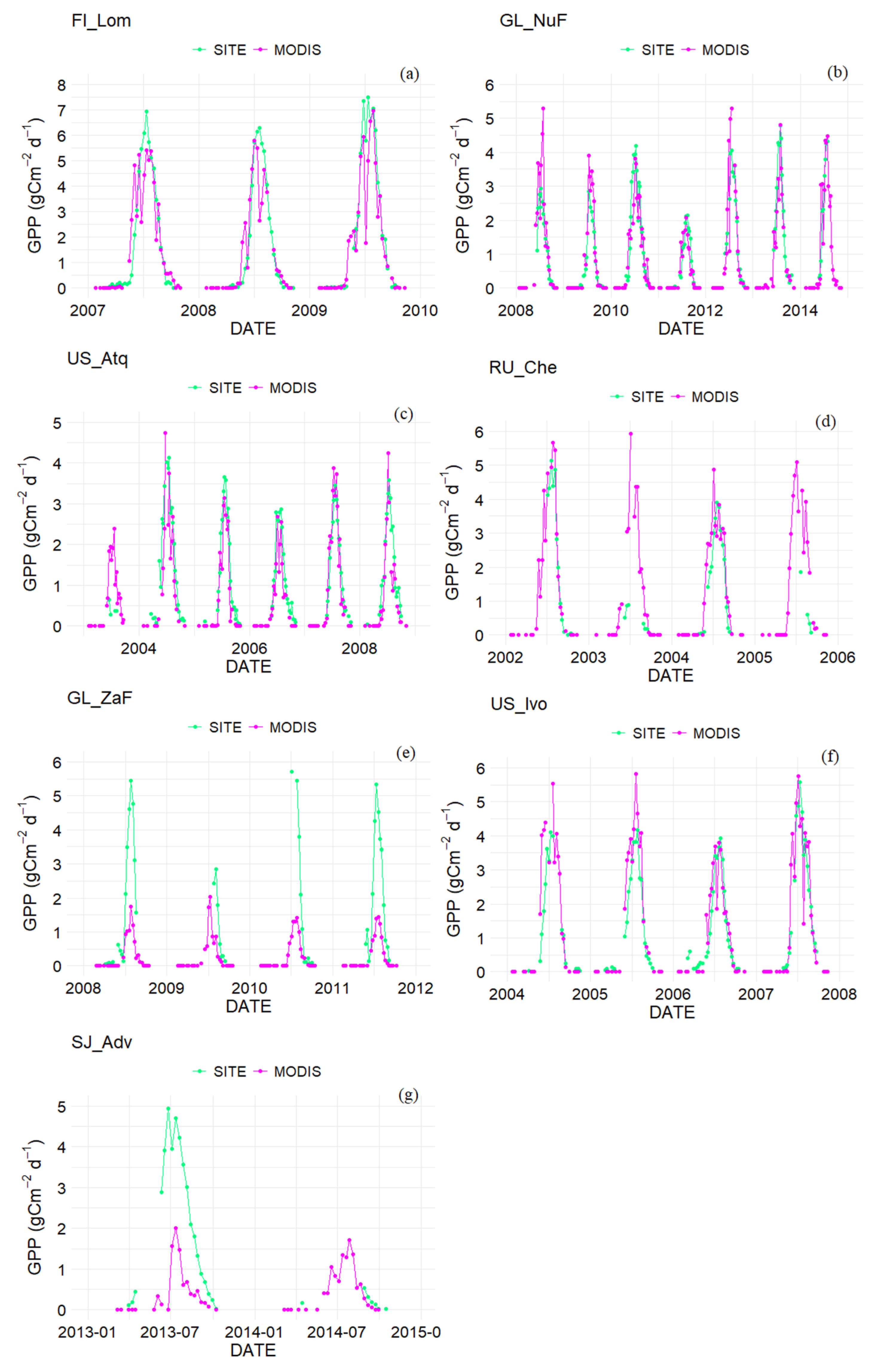
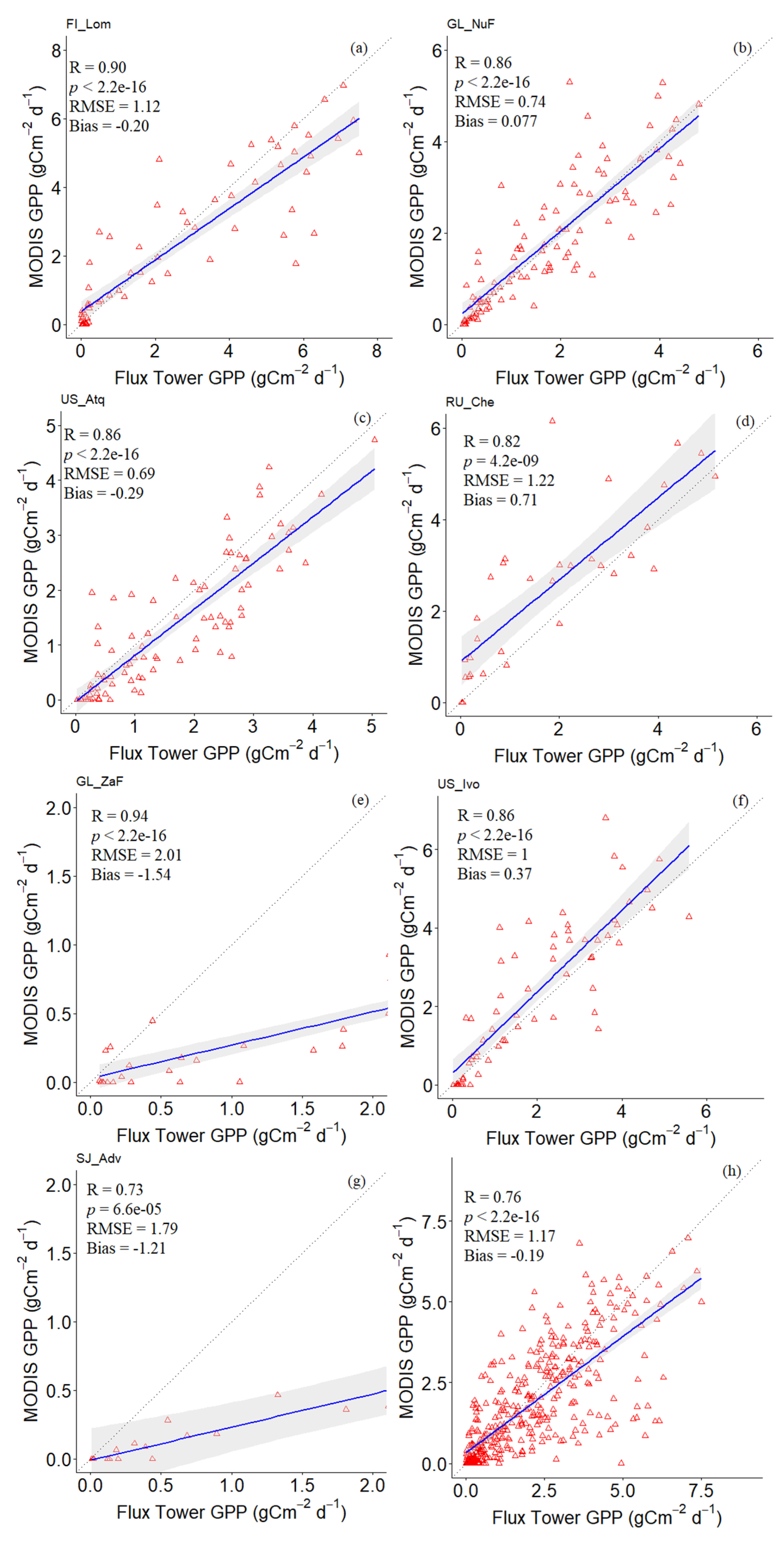
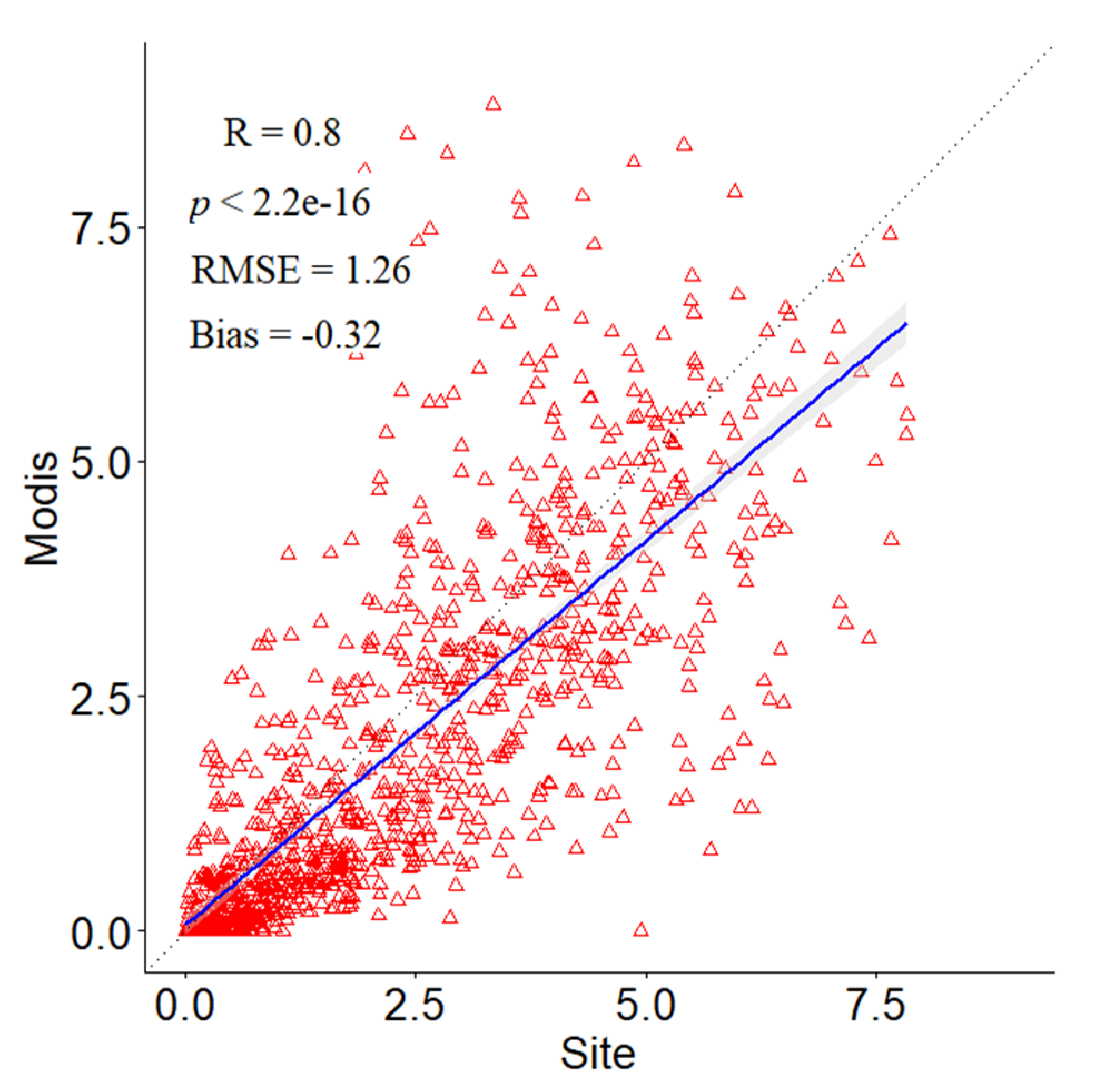
4.1. Validation MOD17A2H Based on In Situ

The results of in situ and MOD17A2H GPP were compared in different land cover types. Figure 2 shows the time series of MOD17A2H and the in situ-based GPP over wetlands; their scatter plots are presented in Figure 3. As shown in Figure 2, missing data occurs frequently in the time series, especially in winter and early spring. This is attributed to the weak photosynthetic activity of vegetation and the lower data coverage during this period. Both MOD17A2H and in situ-based GPP show reasonable seasonal and annual variability over wetlands (Figure 2). However, the agreement between them is significantly different from site to site.
The comparison results over wetlands can be divided into two groups according to the performance of MOD17A2H: (1) FI_Lom, US_Atq, GL_ZaF, and SJ_Adv; and (2) GL_NuF, RU_Che and US_Ivo. MOD17A2H was found to underestimate in group (1) and overestimate in group (2). Nevertheless, the degree of underestimation varies significantly from site to site and is low for FI_lom and US_Atq, both in magnitude and temporal variation trend (Figure 2a,c), with RMSEs of 1.12 and 0.69 g C m−2 d−1 and R of 0.9 and 0.86, respectively (Figure 3a,c). For GL_ZaF and SJ_Adv, the agreement is worse, as the RMSEs are 2.01 and 1.79 g C m−2 d−1, respectively (Figure 3e,g), and the bias is very large, with values of −1.54 and −1.21, respectively. The large discrepancy between MOD17A2H and in situ GPP may be caused by their spatial scale mismatch. Furthermore, it should be noted that the data points (less than 50) over these two sites are very limited. For the second group, MOD17A2H is generally consistent with in situ measurements, with the RMSEs of 0.74, 1.22, and 1.0 g C m−2 d−1, and R of 0.86, 0.82, and 0.86 over GL_NuF, RU_Che, and US_Ivo, respectively.
As indicated by Figure 3, the MOD17A2H performs well over wetlands when excluding the sites with limited data points (i.e., GL_ZaF and SJ_Adv). One interesting observation was that the latitudes of GL_ZaF and SJ_Adv are higher than 74° N while those of the other sites are lower than 74° N. In addition, the GL_NuF site where the best agreement between MOD17A2H and in situ occurs has the lowest latitude of all the wetland sites. Therefore, it can be inferred that the accuracy of MOD17A2H may be related to latitude, as it is higher over low latitudes but lower over high latitudes. When it comes to the overall performance of MOD17A2H over wetlands (Figure 3h), the overall RMSE and R are 1.17 g C m−2 d−1 and 0.76, respectively. MOD17A2H slightly underestimates GPP, with a bias of −0.19. Based on the results above, MOD17A2H can be considered capable of revealing the spatial distribution characteristics and the temporal trend of GPP over wetlands in the Arctic.
Figure 4 and Figure 5 show the evaluation results of MOD17A2H over forest sites (i.e., FI_Sod and US_Prr). MOD17A2H underestimates GPP at FI_Sod but overestimates GPP at US_Prr. The extent of misestimation differs between the two sites and is weak for FI_Sod but strong for US_Prr. Over FI_Sod, MOD17A2H agrees well with in situ measurements (Figure 4a), with the RMSE of 1.33 g C m−2 d−1 and bias of −0.77 (Figure 5a). However, for US_Prr, their agreement is worse (Figure 4b), with the RMSE of 2.05 g C m−2 d−1 and bias of 1.19 (Figure 5b). It is important to note that the extent of misestimating MOD17A2H varies from year to year. This is especially true over US_Prr, where the overestimation of MOD17A2H is more significant from 2012 to 2014 (Figure 4b). Although the two sites feature forests, their locations are different (Table 1), indicating that the accuracy of MOD17A2H is also influenced by other factors. As shown in Figure 5c, although MOD17A2H slightly underestimates GPP over forests (Bias = −0.36), overall, MOD17A2H was consistent with site measurements over forests, with RMSE and R of 1.51 g C m−2 d−1 and 0.79, respectively.
Figure 6 and Figure 7 present the comparison results over grasslands, shrublands, and permanent snow and ice. MOD17A2H generally underestimates GPP over these land cover types but the degree of underestimation varies with sites, as it is relatively weak for RU_Cok (RMSE = 1.02 g C m−2 d−1, Bias = −0.44) but strong for GL_ZaH and SJ_Blv (with the RMSEs of 0.61 and 0.19 g C m−2 d−1 and the Bias of −0.5 and −0.17, respectively). It is important to remember that the latitudes of GL_ZaH and SJ_Blv are higher than at RU_Cok, which further demonstrates that the accuracy of MOD17A2H is related to the latitude of the sites.
When combining the data points of all the sites (Figure 8), MOD17A2H slightly underestimates GPP, with the bias of −0.32. The overall accuracy of MOD17A2H is reasonable over the Arctic, with RMSE of 1.26 g C m−2 d−1 and R of 0.8, respectively. These indicators demonstrate that MOD17A2H is able to capture the spatiotemporal variation characteristics of GPP in the Arctic.
From the validation results based on in situ measurements, it is shown that the MOD17A2H generally underestimates GPP over these land cover types. Nevertheless, depending on the location of the sites, it may underestimate or overestimate GPP within each land cover type. This demonstrates that the accuracy of MOD17A2H is also influenced by other factors in addition to land cover types. For instance, the latitude seems to be associated with the accuracy of MOD17A2H given that the accuracy of MOD17A2H tends to be higher over low latitudes but lower over high latitudes (>74° N), which might be due to the actual maximum radiation conversion efficiency (εmax) of vegetations being quite different from the given εmax in high latitude. In fact, the misclassification of a pixel is also responsible for the inconsistency of the accuracies derived from different sites within the same land cover type. Because the classification scheme adopted by IGBP is too general, it cannot reveal the detailed categories carrying out photosynthesis. Moreover, MOD17A2H is calculated based on the concept of light use efficiency (LUE), which assumes a fixed maximum radiation conversion efficiency (εmax) of each land cover type [19]. This treatment also introduced errors when misclassification occurred. Another cause of the inconsistency is the different degrees of surface heterogeneities within the satellite pixel, which cause the sites to be more or less representative of the satellite pixel. Last but not least, since missing data of in situ may occur unequally during each 8-day period, the temporal representativeness varies across these sites. Despite these uncertainties, the validation results still suggest that the performance of MOD17A2H is better over shrublands and wetlands than it is over forests.

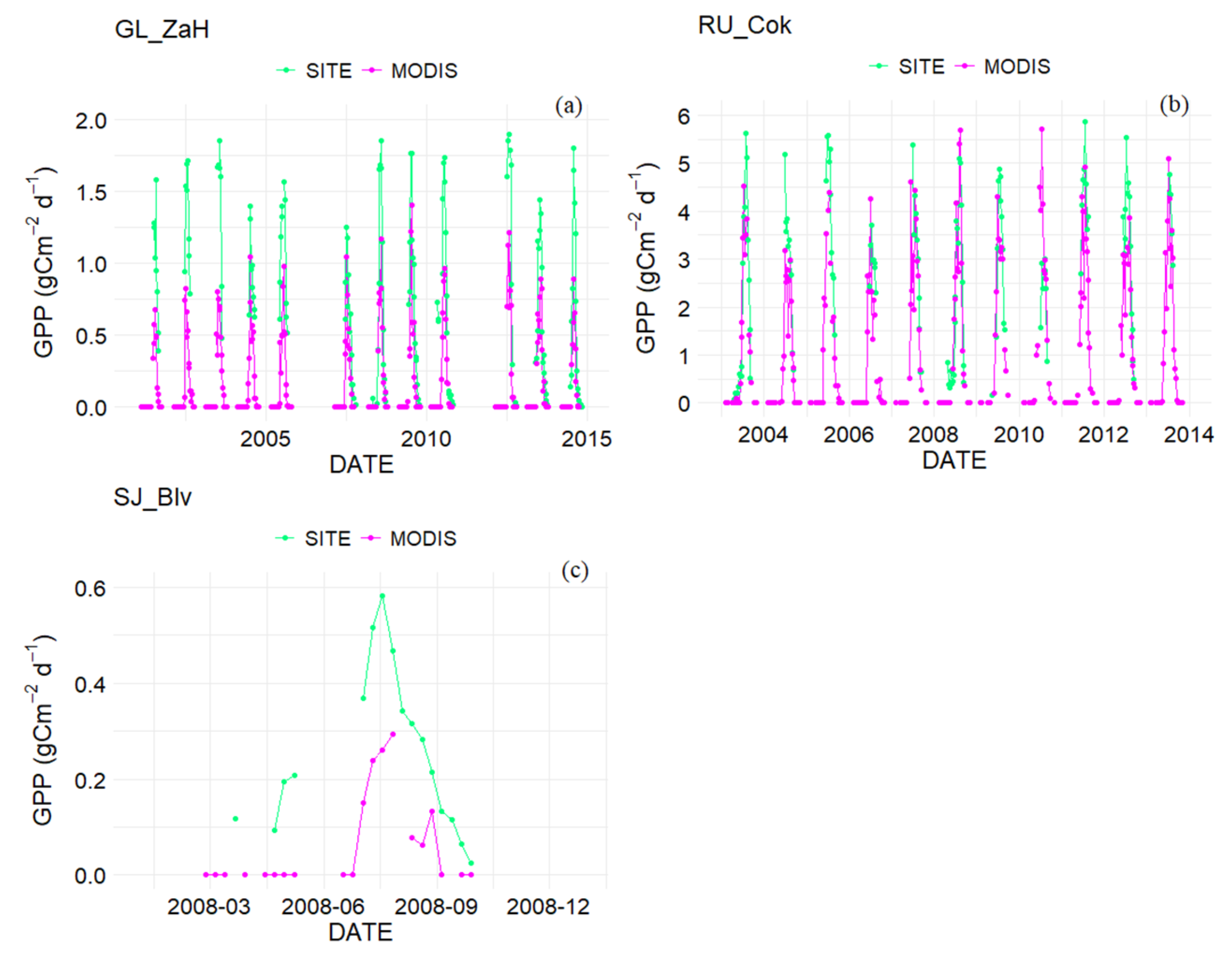
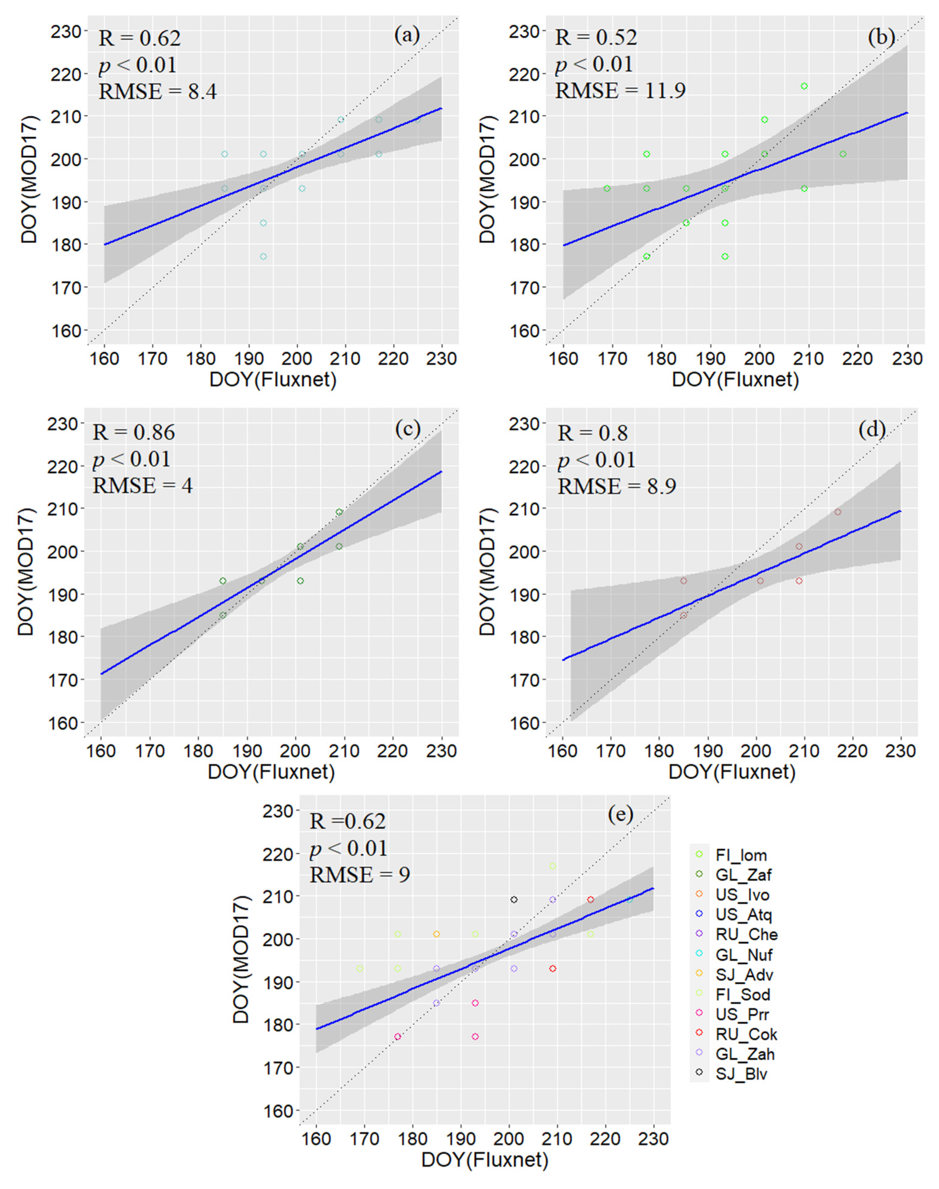
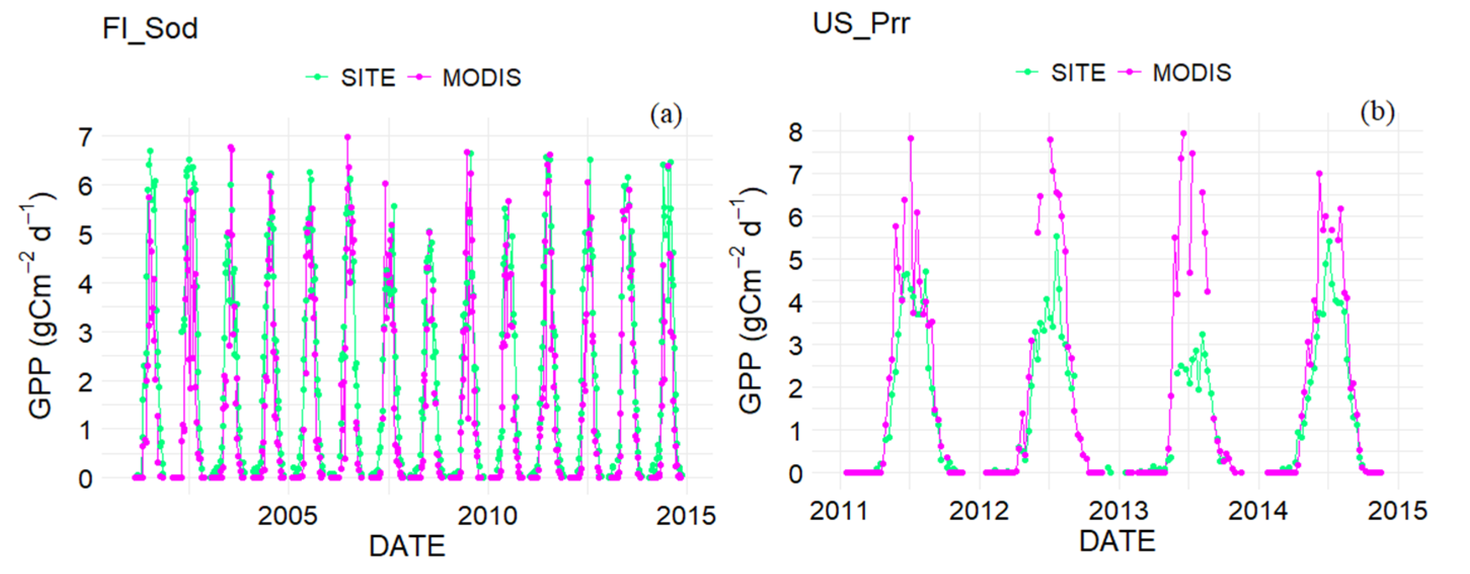
4.2. Evaluation of the Phenological Characteristics of MOD17A2H

According to Figure 9, MOD17A2H does express the phenological characteristics of GPP in the Arctic, with cross-sites R and RMSE of 0.62 and 8.9 days, respectively. In particular, as shown in Figure 9c, the peak GPP timing DOY of grasslands was the most consistent with that extracted from in situ data (R = 0.86, RMSE = 4 days). By contrast, the discrepancy between MOD17A2H and in situ peak GPP timing over forest sites was the highest (Figure 9b), with R and RMSE of 0.52 and 11.9 days, respectively, which demonstrates that the characteristics of the forests (mostly evergreen needleleaf) GPP, derived from MOD17A2H, are difficult to capture compared with the characteristics of other land cover types. This might be due to two reasons: (1) forests are composed of evergreen needleleaf forests, evergreen broadleaf forests, deciduous needleleaf forests, deciduous broadleaf forests, and mixed forests; therefore, the diversity of forests makes phenological characteristics difficult to capture by satellite observations; and (2) evergreen needleleaf forest is one of the major forest types in the Arctic, which is less sensitive to climate changes according to [46], thus the phenological characteristics of evergreen needleleaf forests are hard to capture.

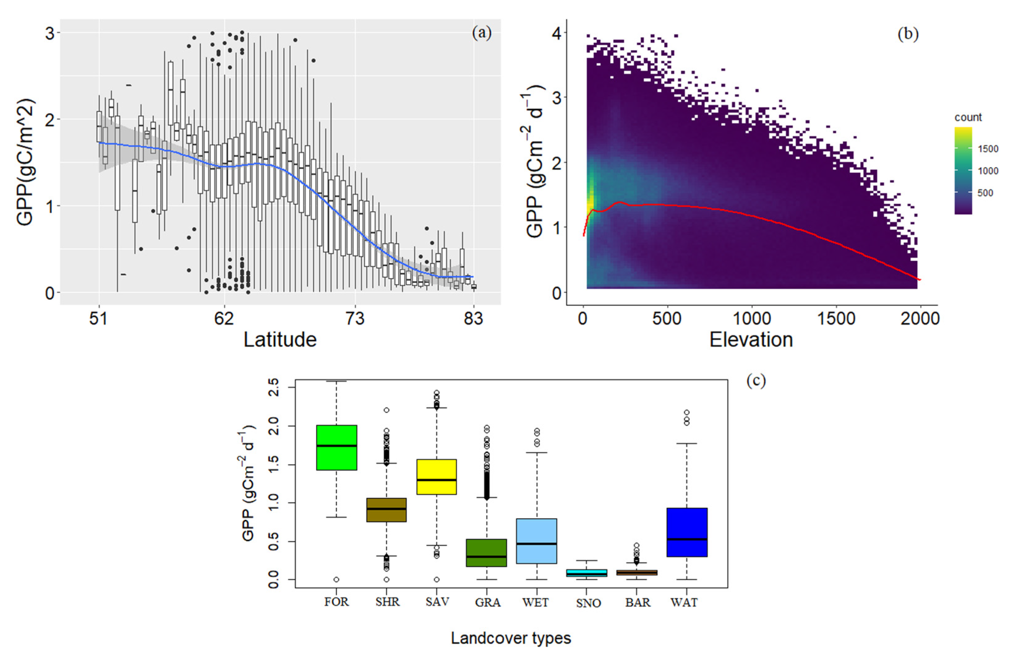
4.3. Spatial Distribution Characteristics

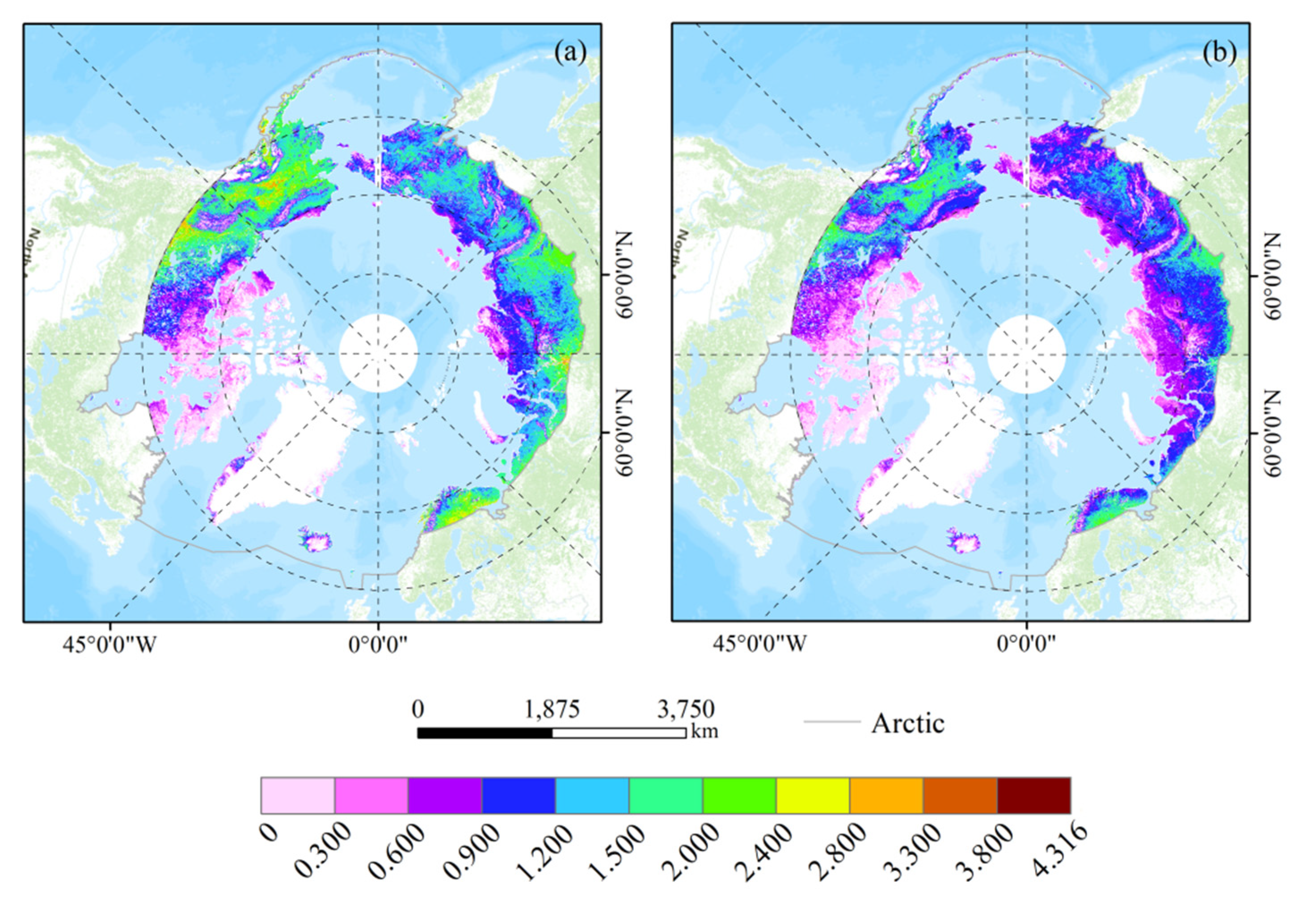
4.3.1. Spatial Distribution of Annual-Averaged GPP

Figure 10 shows the annual maximum (Figure 10a) and annual-averaged GPP (Figure 10b), derived from MOD17A2H, in the Arctic on a pixel basis. The two metrics generally present similar spatial distribution patterns. GPP is relatively low in the northeast of Canada and the regions surrounding Greenland, with an annual-maximum range of 0 to 1.200 g C m−2 d−1 and an annual-averaged range of 0 to 0.900 g C m−2 d−1. The low GPP over these areas can be explained by the fact that these areas are almost completely covered by grassland and barren land, which have lower GPP (Figure 11c). Therefore, it can be inferred that the spatial distribution of GPP is related to land cover types. Furthermore, the GPP shows a decreasing trend as the latitude increases. This is especially true over the eastern hemisphere of the Arctic, where the annual maximum of GPP drops from 3.300 to 0.300 g C m−2 d−1 and the annual-averaged of GPP decreases from 2.400 to 0.300 g C m−2 d−1.
Figure 11a,b display the distribution of GPP with latitude and elevation, respectively. It can be seen that GPP generally shows a decreasing trend with latitude, which is in line with the results of Gounand et al. [25]. Nevertheless, the sensitivity of GPP to latitude depends on the situation. The results define three groups of latitudes: (1) latitudes less than 62° N and more than 80° N; (2) latitudes higher than 62° N but lower than 66° N; and (3) latitudes between 66° N and 80° N. In the first group, the GPP distribution is sparse because the region located within this scope is quite limited. Thus, GPP shows irregular variation patterns with latitude. In the second group, GPP is relatively stable, indicating the insensitivity of GPP to latitude within this scope. Nevertheless, GPP presents a clear decreasing trend in the third group, demonstrating that GPP is most sensitive to latitude from 66° N to 80° N. Similar to latitude, GPP generally shows a decreasing trend with increasing elevation (Figure 11b). However, the decreasing rates are different depending on the elevation, which is smaller for elevations lower than 700 m, but larger for elevations higher than 700 m.
Figure 11c presents the annual-averaged GPP distribution over different land cover types for the entire study period. It can be seen that all land cover types show considerable interannual variation except for permanent snow and ice as well as barren land (as indicated by the wide distribution of boxplots).

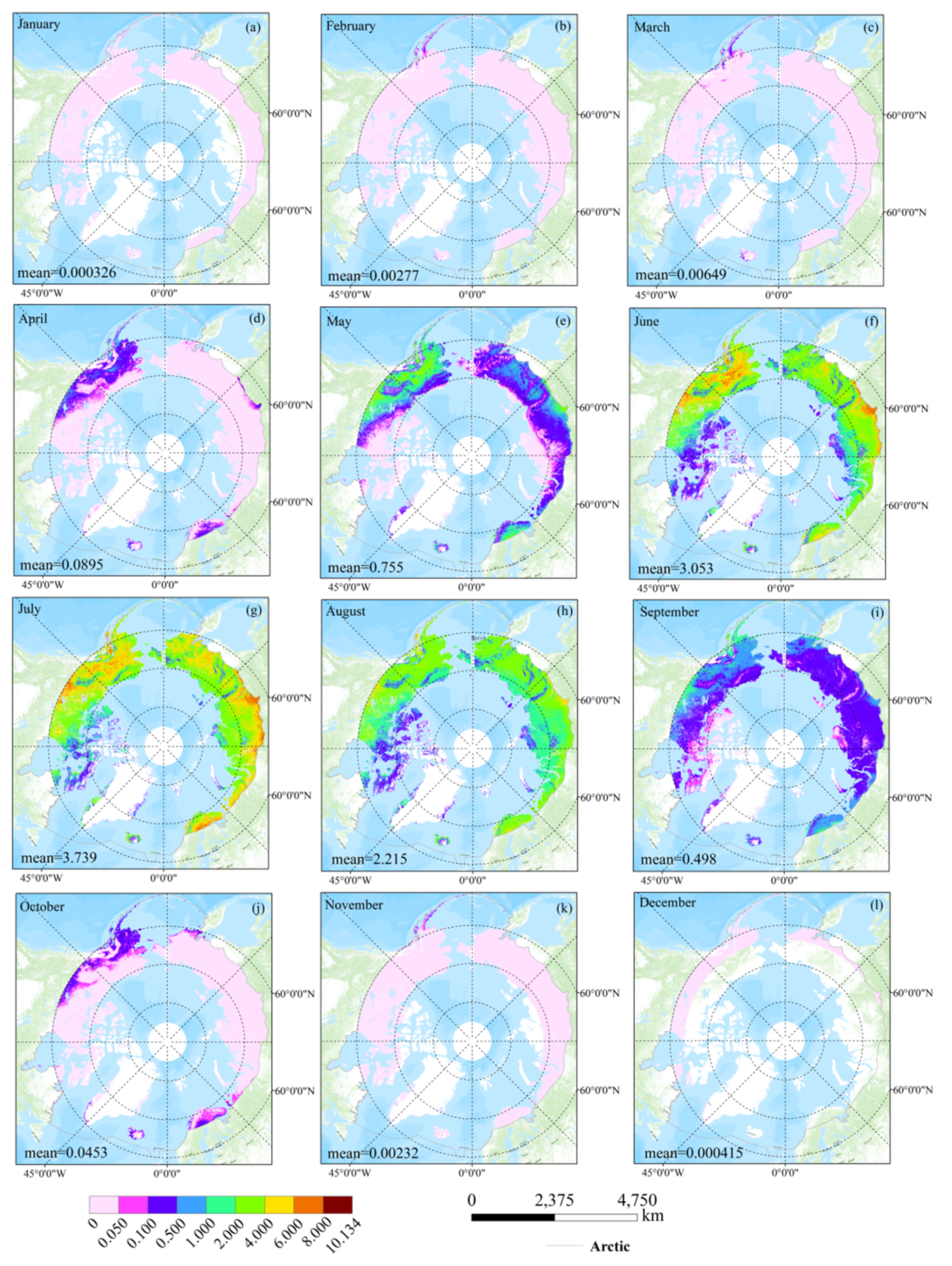
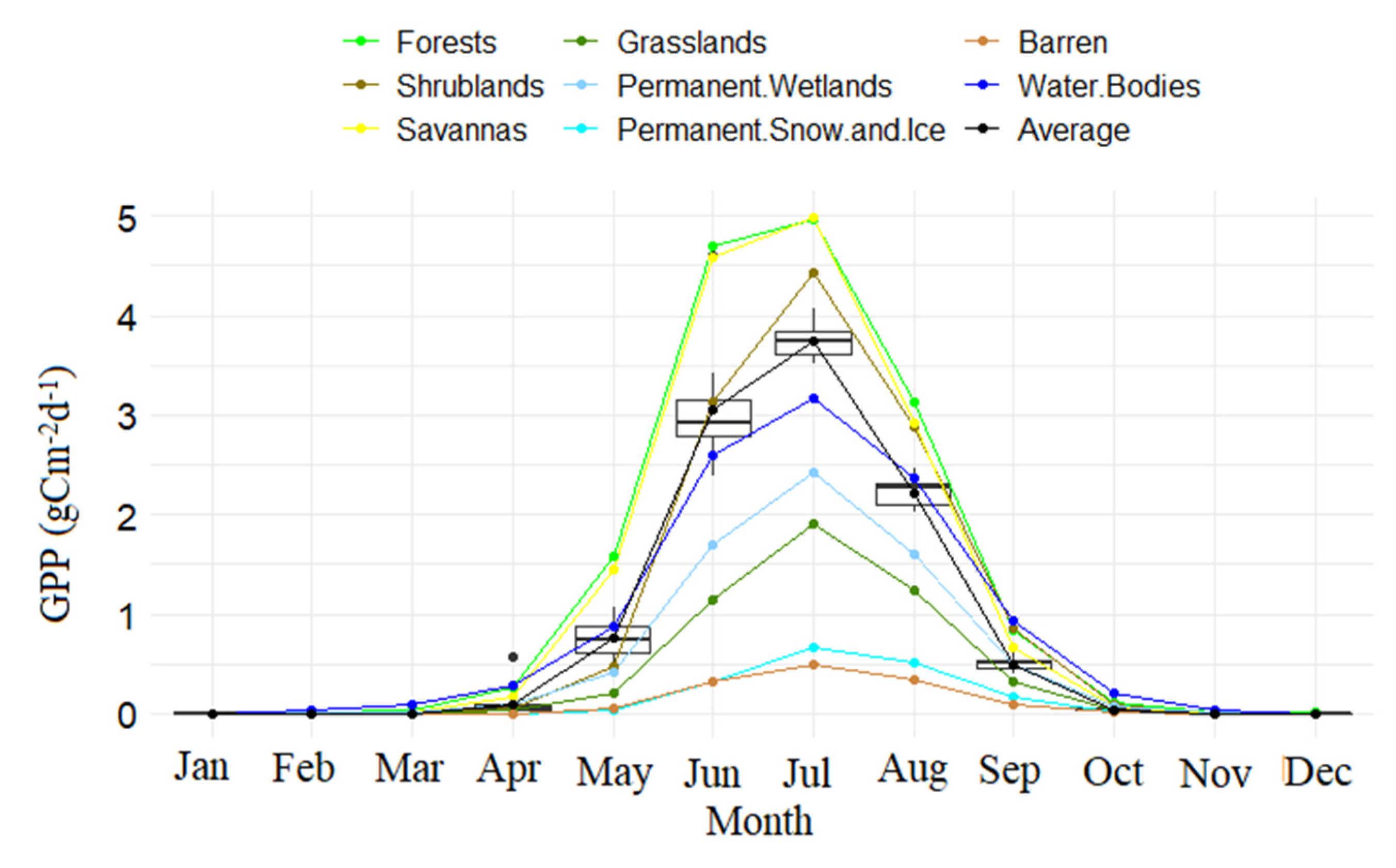
4.3.2. Variation of Monthly GPP

Figure 12 displays the spatial pattern of multiyear (2001–2019) averaged monthly GPP. The phenological cycle of vegetation is clearly shown in the figure. GPP is very low from November to March, with values close to 0. This is because the photosynthesis of vegetation was restricted due to the extremely harsh environment and limited lighting hours. From April to July, with rising temperatures, melting snow and sea ice, and increasing hours of light, the carbon fixation ability of vegetation is stronger, which contributes to the gradual expansion of GPP from the northwest of Canada and the low latitudes of Russia to the entire Arctic. In addition, the mean GPP over the whole Arctic shows a rapid increase during this period, with the values increasing from 0.0859 g C m−2 d−1 in April to 3.739 g C m−2 d−1 in July. However, the GPP gradually decreases from August to October as the mean values decrease from 2.215 to 0.0453 g C m−2 d−1. This may be attributed to the decrease in temperature, the shortening of day-length, and the senescence of vegetation during this period. The northwestern region of Canada, a small low latitude portion of Russia, and the regions surrounding Iceland have the longest growth period since they are the first to begin and the last to stop photosynthesis. Figure 12 demonstrates that spatial heterogeneity is small during the dormant months (from November to March) and the mid and late summer months (July and August) when GPP is consistently small or large, but large during the transition months (April, May, September, and October) and early summer (June). There are two main reasons for this: the first is the spatial difference in land cover types, the second is the temporal difference in climate conditions [47].
The GPP in the Arctic has a distinct seasonality with the greatest values in July (Figure 13). Throughout the year, most land cover types follow the general seasonality of GPP; they are lowest from January to March, begin to increase in April and reach a maximum in July, decrease from then on and fall back to the lowest values in November. Forest and savannas present the largest GPP from April to August, followed by shrublands, water bodies, permanent wetlands, and grasslands (Figure 13). Permanent snow and ice as well as barren land ranks last. Nevertheless, from September to October, water bodies show slightly larger GPP than other land cover types. These results demonstrate that forests and savannas have a rather high carbon storage capacity during the growing season (from April to August) but water bodies are the biggest contributors to carbon fixation from September to October.
The results of Figure 13 are certainly not anticipated because land cover types such as permanent snow and ice, barren land, and water bodies, which cannot carry out photosynthesis, show considerable GPP. This can be explained by the definition of land cover type of IGBP, which is determined by the dominant land cover of a pixel. Water bodies refer to those pixels that are at least 60% covered by permanent water bodies; barren denotes that at least 60% of the pixel is non-vegetated barren (sand, rock, and soil) areas with less than 10% vegetation; permanent Snow and ice means that at least 60% of the pixel is covered by snow and ice for at least 10 months of the year. Therefore, the misclassified part of a pixel is the source of GPP for these three land cover types. From the results above, it is inferred that only extracting the vegetated pixels, as classified by the land cover, will lead to errors in calculating carbon storage in the Arctic.
Figure 13 also shows that the monthly GPP has the widest distribution in June, indicating that the interannual variation of GPP is the most significant in June. This is understandable since vegetation grew at the fastest speed from May to June (indicated by the largest slope) and thus is more affected by climate change.

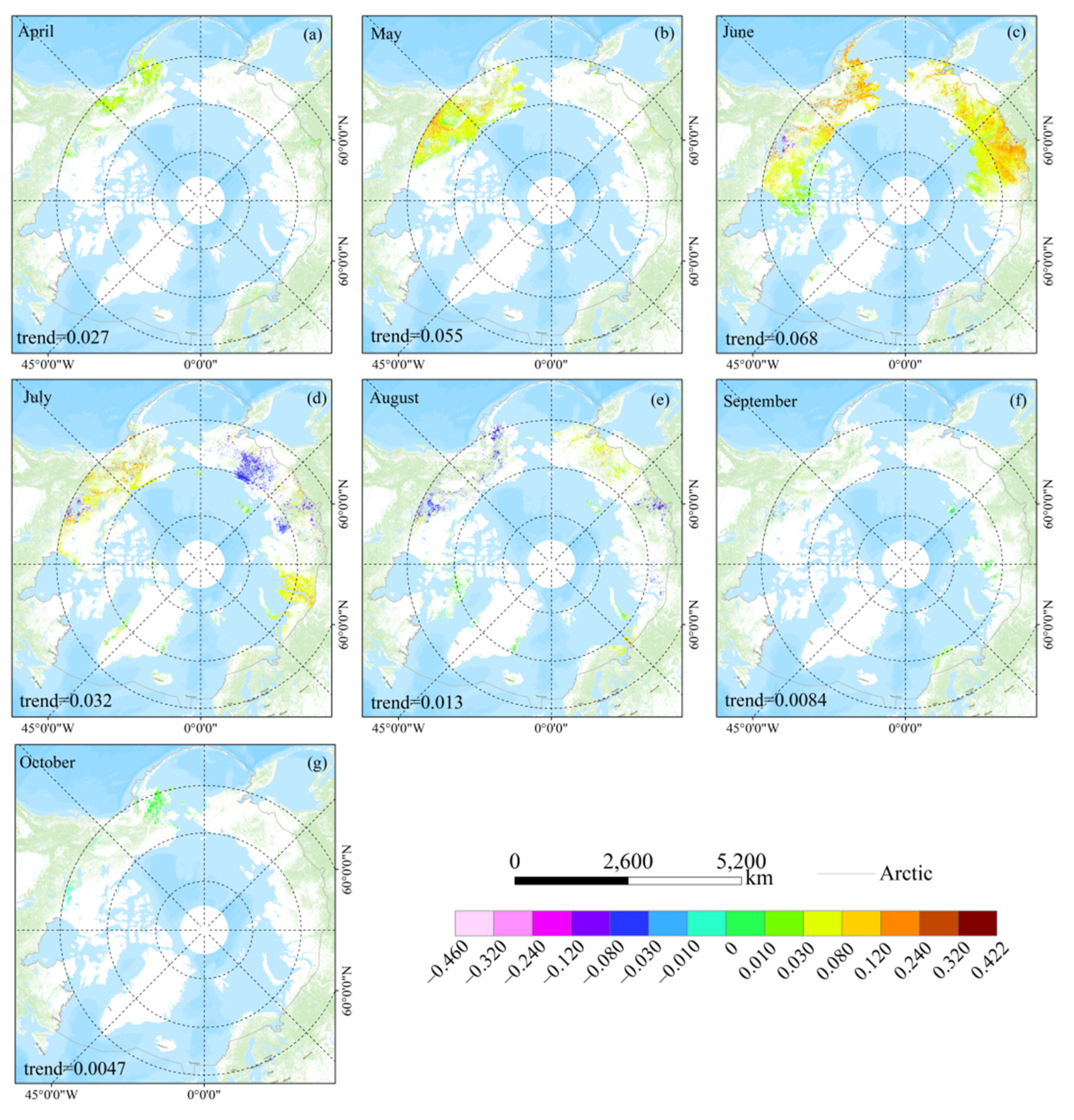
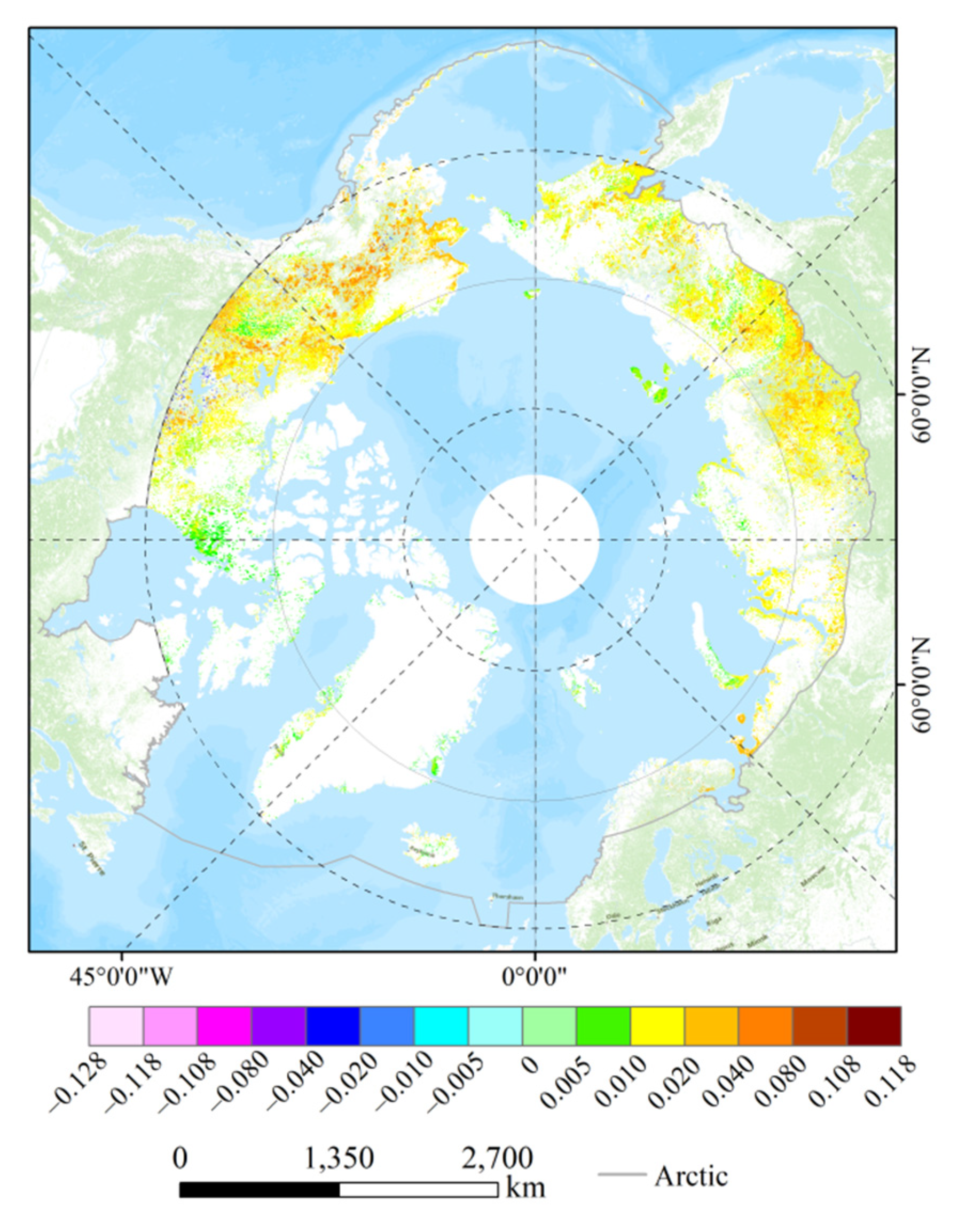
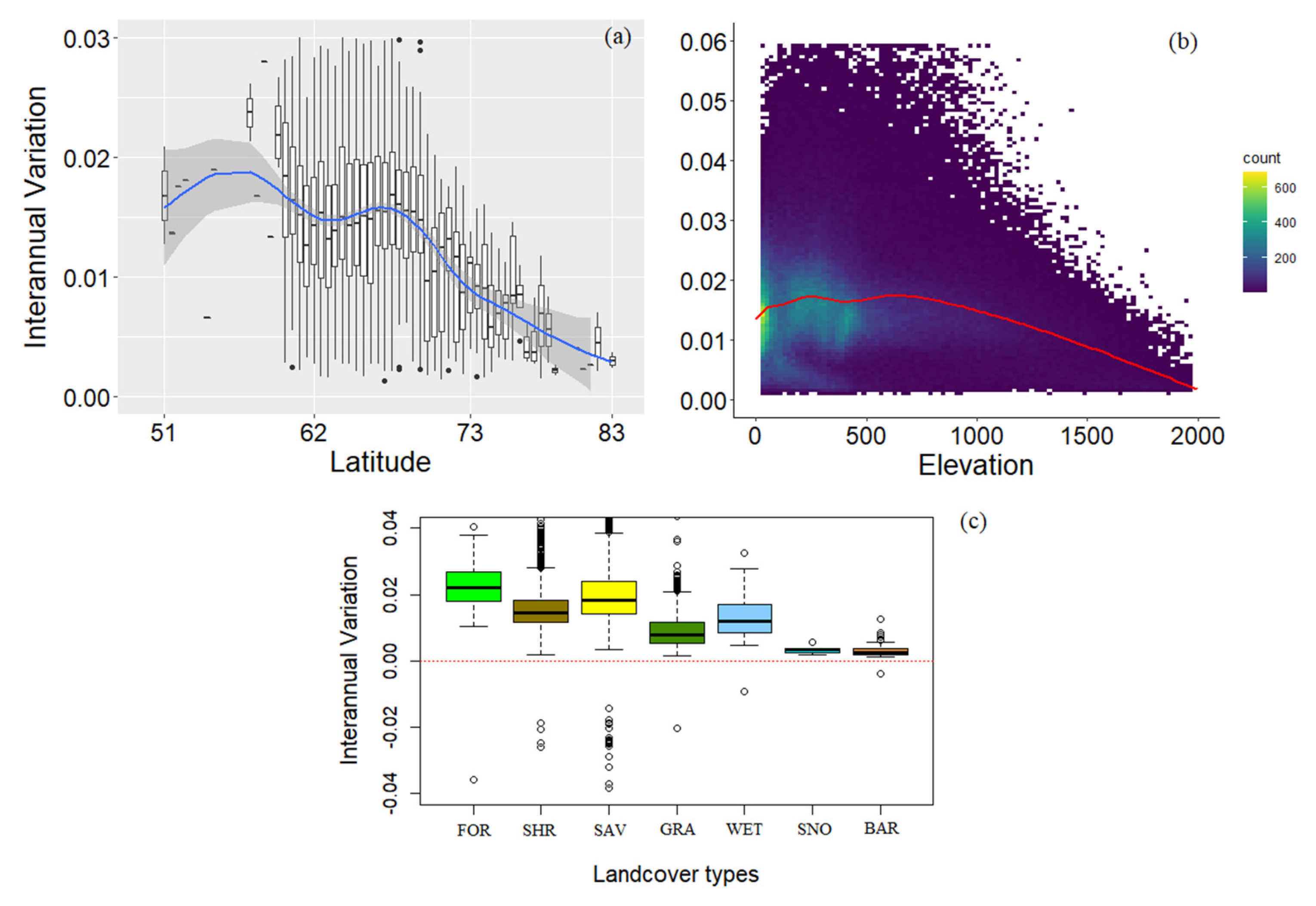
4.4. Trend Estimates of GPP

The interannual variation trend of GPP is shown on a pixel basis (Figure 14); almost half of the Arctic presents significant positive trends, but the magnitude of trends shows distinct spatial variation. In the northwest of Canada and the latitude lower than 70° N of Russia, the trend of GPP varies significantly, ranging from 0.005 to 0.08 g C m−2 year−1. By contrast, in the northeast of Canada and the regions surrounding Greenland, the GPP trend varies slightly, ranging from 0 to 0.01 g C m−2 year−1. The small range of the GPP trend is likely to be associated with grassland and barren land. The former has a relatively small spatial variation, as indicated by the centralized distribution of the interannual trends in GPP. The latter has a very small GPP, which is almost constant over time (Figure 11c).
As seen from Figure 12, there is almost no vegetation productivity in the Arctic from November to March. Thus, Figure 15 only presents the interannual trends from April to October. It is clear that the interannual trends show significant differences between different months. From April to June, the interannual trends in northwestern Canada gradually increase and reach a maximum in June, with an overall trend of 0.068 g C m−2 year−1 (Figure 15c). From then on, the interannual trend decreases gradually until October (Figure 15d–g). Furthermore, we also find that the interannual trends in July and August are more spatially heterogeneous than in other months. These results demonstrate that the response of vegetation to climate change is not consistent between different months and over different areas. It is interesting to find that the interannual trend is the most significant in June (Figure 15c) and shows a similar spatial pattern to the overall interannual trend (Figure 14). This demonstrates that the interannual variations of GPP in the Arctic may be dominated by the change of vegetation productivity in June.
The distributions of the interannual trends in GPP with latitude and elevation are shown in Figure 16a,b. The interannual trends first increase at the latitude of 51° N and reach a maximum of 0.018 g C m−2 year−1 at 57° N. From then on, the interannual trend decreases significantly until 62° N. However, the interannual trend seems to be independent of latitude from 62° N to 66° N. Then a clear decreasing trend can be observed from 66° N until 80° N. Therefore, we can conclude that the interannual trend of GPP is sensitive to the latitude, except in the regions located between 62° N and 66° N, which is similar to the distribution of annual-averaged GPP with the variation of latitude. This is mainly because the regions located between (62° N, 66° N) are in the same climatic zone, namely in the north temperate zone. Figure 16b demonstrates that the interannual trend of GPP generally shows a decreasing trend with increasing elevations. However, the sensitivity is relatively weak at low elevations (<700 m) and significant at larger elevations (>700 m). The low GPP and interannual trend in the regions with relatively higher altitude and latitude Figure 11a,b and Figure 16a,b mainly due to the low precipitation and temperature, which are not conducive to plant growth [48,49]. These results could help us understand the latitude or elevation range in which the change of GPP mainly occurred, providing a basis for understanding the changes of the Arctic GPP.
Figure 16c displays the boxplots of the interannual trends by combining the pixels for each land cover type. It can be seen that almost each land cover type presents positive trends. However, their magnitude, as well as their spatial variation, depend on the land cover types. Forests have the largest interannual trend, followed by savannas and shrublands. The interannual trend of grassland is not as large as we expected and is even slightly smaller than the trend of permanent wetlands. Savannas and forests show the largest spatial variations in interannual trends, as indicated by the most widespread distribution of boxplots. Permanent wetlands and grasslands present the smallest spatial variations when excluding permanent snow and ice as well as barren land. These results demonstrate that the interannual trends of savannas and forests are more influenced by other factors, while those of permanent wetlands and grasslands are less sensitive to other factors.

5. Conclusions

Arctic ecosystems have undergone great changes in the context of climate change. GPP is one of the most crucial indicators of the response of ecosystems to climate change. However, few efforts have been devoted to exploring the spatial variation and phenological characteristics of GPP in the Arctic. In response to this challenge, this study investigated the spatial distribution as well as the seasonal (phenological) and interannual variations of GPP in the Arctic using MOD17A2H. Furthermore, the GPP variation trends with land cover types, latitude, and elevation were also explored. In order to ensure that the results were reliable, the accuracy of MOD17A2H was first evaluated using in situ measurements from FLUXNET.
This study found that MOD17A2H generally underestimates GPP over the land cover types investigated in this study, and its accuracy tends to be higher over low latitude but lower over high latitude. However, the overall accuracy suggests that MOD17A2H is consistent with the FLUXNET 2015 dataset (RMSE = 1.26 g C m−2 d−1, R = 0.8, Bias = −0.32), and MOD17A2H can represent the phenological characteristics of GPP (RMSE = 8.9 days, R = 0.62). Based on MOD17A2H, it was demonstrated that the maximum GPP occurred in July. In addition, the spatial distribution of GPP is related to land cover types; for example, forests and savannas have relatively high carbon storage capacity from April to August. By comparing the GPP variation with latitude and elevation, it was shown that GPP generally decreases as the latitude and elevation increase. However, the phenomenon is not evident for latitudes in the range (62° N, 66° N) and elevation lower than 700 m. The overall trend of GPP in the Arctic is greater than zero and is dominated by the variation of vegetation productivity in June. Furthermore, the response to climate change is different across these land cover types; for example, forests are most sensitive to climate warming. The distribution of the interannual trend in GPP across latitudes and elevations is consistent with the changes in GPP as a function of latitude and elevation.
This study is helpful for understanding the spatiotemporal distribution characteristics of GPP over the Arctic as well as the response of ecosystems to climate change. Nevertheless, the results need to be validated with different satellite products. The number of sites used for validation is limited. Therefore, the presented conclusion about the accuracy of MOD17A2H may not be transferable to other regions. Another limitation is that only individual factors such as land cover type, latitude, and elevation were considered in this paper. Other factors, such as air temperature, precipitation, and snow, that are related to vegetation growth status need to be explored further. This will also be our focus in the future.

Author Contributions

Conceptualization, D.M. and J.W.; methodology, D.M. and X.W.; validation, X.L., C.M. and X.W.; formal analysis, D.M. and X.W; investigation, J.W.; resources, X.W.; data curation, D.M.; writing—original draft preparation, D.M. and X.W.; writing—review and editing, D.M., X.W. and X.M.; visualization, J.W.; supervision, C.M. All authors have read and agreed to the published version of the manuscript.

Funding

This work was jointly supported by the National Key Research and Development Program of China (2019YFA0607003), the National Natural Science Foundation of China (Grant No. 42071296 and 41801226), and the Fundamental Research Funds for the Central Universities (lzujbky-2020-72).

Data Availability Statement

Publicly available datasets were analyzed in this study. This data can be found in Google earth engine platform (https://earthengine.google.com/, accessed on 7 February 2021).

Acknowledgments

We gratefully acknowledge the anonymous reviewers and editor of the paper in providing critical and constructive comments, which has helped us to significantly improve the manuscript. We also appreciate the assistance of the all authors of this paper.

Conflicts of Interest

The authors declare no conflict of interest.

References

  1. Liu, G.M.; Wu, T.H.; Hu, G.J.; Wu, X.D.; Li, W.P. Permafrost existence is closely associated with soil organic matter preservation: Evidence from relationships among environmental factors and soil carbon in a permafrost boundary area. Catena 2021, 196, 104894. [Google Scholar] [CrossRef]
  2. Kug, J.S.; Jeong, J.H.; Jang, Y.S.; Kim, B.M.; Folland, C.K.; Min, S.K.; Son, S.W. Two distinct influences of arctic warming on cold winters over North America and East Asia. Nat. Geosci. 2015, 8, 759–762. [Google Scholar] [CrossRef]
  3. Berra, E.F.; Gaulton, R. Remote sensing of temperate and boreal forest phenology: A review of progress, challenges and opportunities in the intercomparison of in-situ and satellite phenological metrics. For. Ecol. Manag. 2021, 480, 118663. [Google Scholar] [CrossRef]
  4. Zhu, X.Y.; Pei, Y.Y.; Zheng, Z.P.; Dong, J.W.; Zhang, Y.; Wang, J.B.; Chen, L.J.; Doughty, R.B.; Zhang, G.L.; Xiao, X.M. Underestimates of grassland gross primary production in modis standard products. Remote Sens. 2018, 10, 1771. [Google Scholar] [CrossRef] [Green Version]
  5. Sun, Z.; Wang, X.; Yamamoto, H.; Tani, H.; Nie, T.; Oppenheimer, M.; Yohe, G. The effects of spatiotemporal patterns of atmospheric co2 concentration on terrestrial gross primary productivity estimation. Clim. Chang. 2020, 163, 913–930. [Google Scholar] [CrossRef]
  6. Francis, J.A.; Vavrus, S.J. Evidence linking arctic amplification to extreme weather in mid-latitudes. Geophys. Res. Lett. 2012, 39, 39. [Google Scholar] [CrossRef]
  7. Cohen, J.; Screen, J.A.; Furtado, J.C.; Barlow, M.; Whittleston, D.; Coumou, D.; Francis, J.; Dethloff, K.; Entekhabi, D.; Overland, J.; et al. Recent arctic amplification and extreme mid-latitude weather. Nat. Geosci. 2014, 7, 627–637. [Google Scholar] [CrossRef] [Green Version]
  8. Screen, J.A.; Simmonds, I. Amplified mid-latitude planetary waves favour particular regional weather extremes. Nat. Clim. Chang. 2014, 4, 704–709. [Google Scholar] [CrossRef] [Green Version]
  9. Wallace, J.M. Global warming and winter weather. Science 2014, 343, 969. [Google Scholar] [CrossRef]
  10. Kim, J.S.; Kug, J.S.; Jeong, S.J.; Huntzinger, D.N.; Michalak, A.M.; Schwalm, C.R.; Wei, Y.X.; Schaefer, K. Reduced north american terrestrial primary productivity linked to anomalous arctic warming. Nat. Geosci. 2017, 10, 572–576. [Google Scholar] [CrossRef]
  11. Wang, S.H.; Zhang, Y.G.; Ju, W.M.; Qiu, B.; Zhang, Z.Y. Tracking the seasonal and inter-annual variations of global gross primary production during last four decades using satellite near-infrared reflectance data. Sci. Total Environ. 2021, 755, 142569. [Google Scholar] [CrossRef]
  12. Zheng, Y.; Shen, R.Q.; Wang, Y.W.; Li, X.Q.; Liu, S.G.; Liang, S.L.; Chen, J.M.; Ju, W.M.; Zhang, L.; Yuan, W.P. Improved estimate of global gross primary production for reproducing its long-term variation, 1982–2017. Earth Syst. Sci. Data 2020, 12, 2725–2746. [Google Scholar] [CrossRef]
  13. Myrstener, M.; Gomez-Gener, L.; Rocher-Ros, G.; Giesler, R.; Sponseller, R.A. Nutrients influence seasonal metabolic patterns and total productivity of arctic streams. Limnol. Oceanogr. 2021, 66, S182–S196. [Google Scholar] [CrossRef]
  14. May, J.L.; Parker, T.; Unger, S.; Oberbauer, S.F. Short term changes in moisture content drive strong changes in normalized difference vegetation index and gross primary productivity in four arctic moss communities. Remote Sens. Environ. 2018, 212, 114–120. [Google Scholar] [CrossRef]
  15. Ryu, Y.; Baldocchi, D.D.; Kobayashi, H.; van Ingen, C.; Li, J.; Black, T.A.; Beringer, J.; van Gorsel, E.; Knohl, A.; Law, B.E.; et al. Integration of modis land and atmosphere products with a coupled-process model to estimate gross primary productivity and evapotranspiration from 1 km to global scales. Glob. Biogeochem. Cycles 2011, 25, 4. [Google Scholar] [CrossRef] [Green Version]
  16. Xia, J.Y.; Niu, S.L.; Ciais, P.; Janssens, I.A.; Chen, J.Q.; Ammann, C.; Arain, A.; Blanken, P.D.; Cescatti, A.; Bonal, D.; et al. Joint control of terrestrial gross primary productivity by plant phenology and physiology. Proc. Natl. Acad. Sci. USA 2015, 112, 2788–2793. [Google Scholar] [CrossRef] [PubMed] [Green Version]
  17. Ma, X.L.; Huete, A.; Yu, Q.; Restrepo-Coupe, N.; Beringer, J.; Hutley, L.B.; Kanniah, K.D.; Cleverly, J.; Eamus, D. Parameterization of an ecosystem light-use-efficiency model for predicting savanna gpp using modis evi. Remote Sens. Environ. 2014, 154, 253–271. [Google Scholar] [CrossRef]
  18. Heinsch, F.A.; Zhao, M.S.; Running, S.W.; Kimball, J.S.; Nemani, R.R.; Davis, K.J.; Bolstad, P.V.; Cook, B.D.; Desai, A.R.; Ricciuto, D.M.; et al. Evaluation of remote sensing based terrestrial productivity from modis using regional tower eddy flux network observations. IEEE Trans. Geosci. Remote Sens. 2006, 44, 1908–1925. [Google Scholar] [CrossRef] [Green Version]
  19. Sjostrom, M.; Zhao, M.; Archibald, S.; Arneth, A.; Cappelaere, B.; Falk, U.; de Grandcourt, A.; Hanan, N.; Kergoat, L.; Kutsch, W.; et al. Evaluation of modis gross primary productivity for africa using eddy covariance data. Remote Sens. Environ. 2013, 131, 275–286. [Google Scholar] [CrossRef]
  20. Kanniah, K.D.; Beringer, J.; Hutley, L.B.; Tapper, N.J.; Zhu, X. Evaluation of collections 4 and 5 of the modis gross primary productivity product and algorithm improvement at a tropical savanna site in northern australia. Remote Sens. Environ. 2009, 113, 1808–1822. [Google Scholar] [CrossRef]
  21. Wang, J.M.; Sun, R.; Zhang, H.L.; Xiao, Z.Q.; Zhu, A.R.; Wang, M.J.; Yu, T.; Xiang, K.L. New global musyq gpp/npp remote sensing products from 1981 to 2018. IEEE J. Sel. Top. Appl. Earth Obs. Remote Sens. 2021, 14, 5596–5612. [Google Scholar] [CrossRef]
  22. O’Sullivan, M.; Smith, W.K.; Sitch, S.; Friedlingstein, P.; Arora, V.K.; Haverd, V.; Jain, A.K.; Kato, E.; Kautz, M.; Lombardozzi, D.; et al. Climate-driven variability and trends in plant productivity over recent decades based on three global products. Glob. Biogeochem. Cycles 2020, 34, 34. [Google Scholar]
  23. Yu, T.; Sun, R.; Xiao, Z.Q.; Zhang, Q.; Liu, G.; Cui, T.X.; Wang, J.M. Estimation of global vegetation productivity from global land surface satellite data. Remote Sens. 2018, 10, 327. [Google Scholar] [CrossRef] [Green Version]
  24. Tang, X.G.; Li, H.P.; Huang, N.; Li, X.Y.; Xu, X.B.; Ding, Z.; Xie, J. A comprehensive assessment of modis-derived GPP for forest ecosystems using the site-level FLUXNET database. Environ. Earth Sci. 2015, 74, 5907–5918. [Google Scholar] [CrossRef]
  25. Gounand, I.; Little, C.J.; Harvey, E.; Altermatt, F. Global quantitative synthesis of ecosystem functioning across climatic zones and ecosystem types. Glob. Ecol. Biogeogr. 2020, 29, 1139–1176. [Google Scholar] [CrossRef]
  26. Fisher, J.I.; Mustard, J.F. Cross-scalar satellite phenology from ground, Landsat, and MODIS data. Remote Sens. Environ. 2007, 109, 261–273. [Google Scholar] [CrossRef]
  27. Xu, X.J.; Zhou, G.M.; Du, H.Q.; Mao, F.J.; Xu, L.; Li, X.J.; Liu, L.J. Combined modis land surface temperature and greenness data for modeling vegetation phenology, physiology, and gross primary production in terrestrial ecosystems. Sci. Total Environ. 2020, 726, 137948. [Google Scholar] [CrossRef] [PubMed]
  28. Yang, S.S.; Zhang, J.H.; Zhang, S.; Wang, J.W.; Bai, Y.; Yao, F.M.; Guo, H.D. The potential of remote sensing-based models on global water-use efficiency estimation: An evaluation and intercomparison of an ecosystem model (BESS) and algorithm (MODIS) using site level and upscaled eddy covariance data. Agr. Forest Meteorol. 2020, 287, 107959. [Google Scholar] [CrossRef]
  29. Reichstein, M.; Falge, E.; Baldocchi, D.; Papale, D.; Aubinet, M.; Berbigier, P.; Bernhofer, C.; Buchmann, N.; Gilmanov, T.; Granier, A.; et al. On the separation of net ecosystem exchange into assimilation and ecosystem respiration: Review and improved algorithm. Glob. Chang. Biol. 2005, 11, 1424–1439. [Google Scholar] [CrossRef]
  30. Lasslop, G.; Reichstein, M.; Papale, D.; Richardson, A.D.; Arneth, A.; Barr, A.; Stoy, P.; Wohlfahrt, G. Separation of net ecosystem exchange into assimilation and respiration using a light response curve approach: Critical issues and global evaluation. Glob. Chang. Biol. 2010, 16, 187–208. [Google Scholar] [CrossRef] [Green Version]
  31. Monteith, J.L. Solar radiation and productivity in tropical ecosystems. J. Appl. Ecol. 1972, 9, 747–766. [Google Scholar] [CrossRef] [Green Version]
  32. Running, S.W.; Zhao, M. User’s Guide Daily GPP and Annual NPP (MOD17A2H/A3H) and Year-end Gap-Filled (MOD17A2HGF/A3HGF) Products NASA Earth Observing System MODIS Land Algorithm (For Collection 6). 2019. Available online: https://landweb.modaps.eosdis.nasa.gov/QA_WWW/forPage/user_guide/MOD17UsersGuide2019.pdf (accessed on 15 July 2021).
  33. Liang, D.; Zuo, Y.; Huang, L.S.; Zhao, J.L.; Teng, L.; Yang, F. Evaluation of the consistency of modis land cover product (mcd12q1) based on chinese 30 m globeland30 datasets: A case study in Anhui Province, China. ISPRS Int. J. Geo-Inf. 2015, 4, 2519–2541. [Google Scholar] [CrossRef] [Green Version]
  34. Yamazaki, D.; Ikeshima, D.; Tawatari, R.; Yamaguchi, T.; O’Loughlin, F.; Neal, J.C.; Sampson, C.C.; Kanae, S.; Bates, P.D. A high-accuracy map of global terrain elevations. Geophys. Res. Lett. 2017, 44, 5844–5853. [Google Scholar] [CrossRef] [Green Version]
  35. McClean, F.; Dawson, R.; Kilsby, C. Implications of using global digital elevation models for flood risk analysis in cities. Water Resour. Res. 2020, 56, 56. [Google Scholar] [CrossRef]
  36. Uuemaa, E.; Ahi, S.; Montibeller, B.; Muru, M.; Kmoch, A. Vertical accuracy of freely available global digital elevation models (ASTER, AW3D30, MERIT, TanDEM-X, SRTM, and NASADEM). Remote Sens. 2020, 12, 3482. [Google Scholar] [CrossRef]
  37. Hao, S.R.; Jiang, L.M.; Shi, J.C.; Wang, G.X.; Liu, X.J. Assessment of modis-based fractional snow cover products over the Tibetan plateau. IEEE J. Sel. Top. Appl. Earth Obs. Remote Sens. 2019, 12, 533–548. [Google Scholar] [CrossRef]
  38. Yang, J.T.; Jiang, L.M.; Menard, C.B.; Luojus, K.; Lemmetyinen, J.; Pulliainen, J. Evaluation of snow products over the Tibetan plateau. Hydrol. Process. 2015, 29, 3247–3260. [Google Scholar] [CrossRef]
  39. Mir, R.A.; Jain, S.K.; Saraf, A.K.; Goswami, A. Accuracy assessment and trend analysis of modis-derived data on snow-covered areas in the Sutlej basin, Western Himalayas. Int. J. Remote Sens. 2015, 36, 3837–3858. [Google Scholar] [CrossRef]
  40. Ueyama, M.; Iwata, H.; Harazono, Y.; Euskirchen, E.S.; Oechel, W.C.; Zona, D. Growing season and spatial variations of carbon fluxes of Arctic and Boreal ecosystems in Alaska (USA). Ecol. Appl. 2013, 23, 1798–1816. [Google Scholar] [CrossRef]
  41. Wu, X.D.; Wen, J.G.; Xiao, Q.; You, D.Q.; Dou, B.; Lin, X.; Hueni, A. Accuracy assessment on modis (v006), glass and Musyq land-surface albedo products: A case study in the heihe river basin, china. Remote Sens. 2018, 10, 2045. [Google Scholar] [CrossRef] [Green Version]
  42. Li, P.X.; Zhu, W.Q.; Xie, Z.Y. Diverse and divergent influences of phenology on herbaceous aboveground biomass across the tibetan plateau alpine grasslands. Ecol. Indic. 2021, 121, 107036. [Google Scholar] [CrossRef]
  43. De Castro, H.C.; de Carvalho, O.A.; de Carvalho, O.L.F.; de Bem, P.P.; de Moura, R.D.; de Albuquerque, A.O.; Silva, C.R.; Ferreira, P.H.G.; Guimaraes, R.F.; Gomes, R.A.T. Rice crop detection using lstm, bi-lstm, and machine learning models from sentinel-1 time series. Remote Sens. 2020, 12, 2655. [Google Scholar]
  44. Yue, S.; Wang, C.Y. The mann-kendall test modified by effective sample size to detect trend in serially correlated hydrological series. Water Resour. Manag. 2004, 18, 201–218. [Google Scholar] [CrossRef]
  45. Gorelick, N.; Hancher, M.; Dixon, M.; Ilyushchenko, S.; Thau, D.; Moore, R. Google Earth engine: Planetary-scale geospatial analysis for everyone. Remote Sens. Environ. 2017, 202, 18–27. [Google Scholar] [CrossRef]
  46. Lu, L.; Guo, H.; Kuenzer, C.; Klein, I.; Zhang, L.; Li, X. Analyzing phenological changes with remote sensing data in Central Asia. IOP Conf. Ser. Earth Environ. Sci. 2014, 17, 012005. [Google Scholar] [CrossRef]
  47. Korner, C. The use of ‘altitude’ in ecological research. Trends Ecol. Evol. 2007, 22, 569–574. [Google Scholar] [CrossRef]
  48. Kato, T.; Tang, Y.H. Spatial variability and major controlling factors of co2 sink strength in asian terrestrial ecosystems: Evidence from eddy covariance data. Glob. Chang. Biol. 2008, 14, 2333–2348. [Google Scholar] [CrossRef]
  49. Yu, G.R.; Zhu, X.J.; Fu, Y.L.; He, H.L.; Wang, Q.F.; Wen, X.F.; Li, X.R.; Zhang, L.M.; Zhang, L.; Su, W.; et al. Spatial patterns and climate drivers of carbon fluxes in terrestrial ecosystems of China. Glob. Chang. Biol. 2013, 19, 798–810. [Google Scholar] [CrossRef]
Figure 1. (a) Location of the FLUXNET sites used in this study. The description of these sites is provided in Table 1. The base map is the land cover types of the Arctic. (b) The elevation distribution of the Arctic.
Remotesensing 13 02875 g001
Figure 2. Time series comparison between site-based GPP and MOD17A2H over wetland sites, (ag) refers to FI_Lom, GL_NuF, US_Atq, RU_Che, GL_ZaF, US_Ivo and SJ_Adv, respectively.
Remotesensing 13 02875 g002
Figure 3. Scatter plots of site-based GPP against MOD17A2H over different wetland sites (ag) and the overall scatter plots by combining all wetland sites (h). Flux tower GPP means in situ GPP. The gray belt refers to the confidence interval of 95%.
Remotesensing 13 02875 g003
Figure 4. Time series comparison between site-based GPP and MOD17A2H over forest sites, (a) and (b) refers to FI_Sod and US_Prr.
Remotesensing 13 02875 g004
Figure 5. Scatter plots of site-based GPP against MOD17A2H over different forest sites (a,b), and the overall scatter plots by combining all forest sites (c). Flux tower GPP means in situ GPP. Gray belt refers to the confidence interval of 95%.
Remotesensing 13 02875 g005
Figure 6. Time series comparison between site-based GPP and MOD17A2H over grasslands (a), shrublands (b), and permanent snow and ice (c) sites.
Remotesensing 13 02875 g006
Figure 7. Scatter plots of site-based GPP against MOD17A2H over grasslands (a), shrublands (b), permanent snow and ice (c) sites. Flux tower GPP means in situ GPP. Gray belt refers to the confidence interval of 95%.
Remotesensing 13 02875 g007
Figure 8. The overall scatterplots of in situ based GPP against MOD17A2H. Flux tower GPP means in situ GPP. Gray belt refers to the confidence interval of 95%.
Remotesensing 13 02875 g008
Figure 9. The DOY comparison of the timing of the maximum GPP between the sites and MOD17A2H. (ae) Represent permanent wetlands, forests, grasslands, shrublands, and all sites combined, respectively. The gray belt refers to the confidence interval of 95%.
Remotesensing 13 02875 g009
Figure 10. The spatial distribution characteristics of annual-maximum (a) and annual-averaged GPP (b) over the Arctic. Units of GPP are g C m−2 d−1.
Remotesensing 13 02875 g010
Figure 11. The annual-averaged GPP distribution with latitude (a) and elevation (m) (b) for the whole Arctic. The gray belt refers to the confidence interval of 95%, the blue line refers to the fit line, and the boxplots denote the distribution of the annual-averaged GPP with the latitude. (c) The annual-averaged GPP distribution for the entire study period 2001–2019 over different land cover types. FOR, SHR, SAV, GRA, WET, SNO, BAR, and WAT denote the forests, shrublands, savannas, grasslands, permanent wetlands, permanent snow and ice, barren, and water bodies, respectively.
Remotesensing 13 02875 g011
Figure 12. Spatial distribution characteristics of the multiyear averaged monthly GPP over the Arctic, (al) refers to January to December. The mean values of the whole Arctic are also shown in the figure for each month. Units of GPP are g C m−2 d−1.
Remotesensing 13 02875 g012
Figure 13. Multiyear averaged monthly GPP distribution over the entire study period for different land cover types (denoted by colored lines) over the Arctic. The black boxplots denote the multiyear monthly GPP distribution of all land cover types.
Remotesensing 13 02875 g013
Figure 14. The spatial distribution of interannual trend of GPP (g C m−2 year−1) over the Arctic (at 97.5% confidence level based on MK test).
Remotesensing 13 02875 g014
Figure 15. Spatial distribution of the interannual variation trend (g C m−2 year−1) of monthly GPP over the Arctic, (ag) refers to April to October.
Remotesensing 13 02875 g015
Figure 16. Interannual variation trend of GPP (g C m−2 year−1) distribution with latitude (a), elevation (m) (b) over the Arctic. The gray belt refers to the confidence interval of 95%, the blue line refers to the fit line, and the boxplots denote the distribution of the annual-averaged GPP with the latitude. (c) Land cover-dependent interannual variation trend of GPP (g C m−2 year−1) over the Arctic. FOR, SHR, SAV, GRA, WET, SNO, and BAR denote the forests, shrublands, savannas, grasslands, permanent wetlands, permanent snow and ice, barren, and water bodies, respectively.
Remotesensing 13 02875 g016
Table 1. Basic information regarding the FLUXNET sites of the Arctic.
Site_IDSite_NameCountryLatitude (° N)Longitude (° E)Land CoverN
FI-LomLompolojankkaFinland67.997224.2092WET71
GL-NuFNuuk FenGreenland64.1308−251.3861WET105
GL-ZaFZackenberg FenGreenland74.4814−20.5545WET42
RU-CheCherskiRussia68.6130161.3414WET33
SJ-AdvAdventdalenSvalbard and Jan Mayen78.186015.9230WET23
US-AtqAtqasukUSA70.4696−157.4089WET88
US-IvoIvotukUSA68.4865−155.7503WET68
FI-SodSodankylaFinland67.362426.6386ENF371
US-PrrPoker Flat Research Range Black Spruce ForestUSA65.1237−147.4876ENF98
GL-ZaHZackenberg HeathGreenland74.4733−20.5503GRA137
RU-CokChokurdakhRussia70.8291147.4943OSH107
SJ-BlvBayelva, SpitsbergenSvalbard and Jan Mayen78.921711.8311SNO13
WET: wetlands; ENF: evergreen needleleaf forests; GRA: grasslands; OSH: open shrublands; SNO: permanent snow and ice. N means the numbers of the data points of the sites after quality control.
Publisher’s Note: MDPI stays neutral with regard to jurisdictional claims in published maps and institutional affiliations.

