Abstract
A band-to-band mis-registration (BBMR) error often occurs in remote sensing (RS) images acquired by multi-spectral push broom spectrometers such as the Sentinel-2 Multi-spectral Instrument (MSI), leading to adverse impacts on the reliability of further RS applications. Although the systematic band-to-band registration conducted during the image production process corrects most BBMR errors, there are still quite a few images being observed with discernible BBMR. Thus, a quick BBMR detection method is needed to assess the quality of online RS products. We here propose a hybrid framework for detecting BBMR between the visible bands in MSI images. This framework comprises three main steps: first, candidate chips are captured based on Google Earth Engine (GEE) spatial analysis functions to shrink the valid areas inside image scenes as potential target chips. The redundant data pertaining to the local operation process are thus narrowed down. Second, spectral abnormal areas are precisely extracted from inside every single chip, excluding the influences of clouds and water surfaces. Finally, the abnormal areas are matched pixel by pixel between bands, and the best-fit coordinates are then determined to compare with tolerance. Here, the proposed method was applied to 71,493 scenes of MSI Level-1C images covering China and its surrounding areas on the GEE platform. From these images, 4356 chips from 442 scenes were detected with inter-band offsets among the visible bands. Further manual visual inspection revealed that the proposed method had an accuracy of 98.07% at the chip scale and 88.46% at the scene scale.
1. Introduction
The band-to-band mis-registration (BBMR) of multi-spectral remote sensing (RS) images refers to the misalignment between bands caused by differences in the imaging time or angle between detection elements [1]. BBMR has an adverse impact on the reliability of RS applications [2,3], such as target recognition, land-cover classification, and change detection [4]. In particular, appreciably more false information is generated if BBMR occurs over areas with higher spectral complexity. For multi-spectral push broom spectrometers without a beam splitter, e.g., the Sentinel-2 Multi-spectral Instrument (MSI), different spectral band stripe filters are mounted on every single detector. This imposes a slight time offset between each spectral channel sensor during imaging [5], where long-track displacement is approximately 14 km for MSI images [6]. After systematic band-to-band registration (BBR), the inter-band geometric displacement of MSI images should be under 0.3 pixels at 99.7% confidence [7]. However, the pre-processing routine does not necessarily correct all of the displacements, as evidenced by the fact that images with visible inter-band displacement have been observed [8] and have been reported in the Sentinel-2 data quality reports [9]. MSI images have been widely used in a broad range of earth observation applications due to their high revisit frequency (five days at the equator with Sentinel-2A/B), spatial resolution (10 m for visible bands), and radiometric performance [10,11]. Therefore, a robust method is needed to identify MSI images with obvious BBMR errors.
The Sentinel-2 system is designed for high geometrical and spectral measuring performance with ongoing multi-spectral images: approximately 10,000 MSI images can be acquired daily with its twin-satellite capability, and as of July 2020, ~20 million products have been made available. With the support of Google Earth Engine (GEE)—a cloud platform that hosts petabyte-scale geospatial datasets—MSI images and their derivatives have played a crucial role in the global environment and security monitoring [12,13,14,15]. Some BBMR detection methods have been promoted targeting different types of platforms. Therefore, determining whether or not a single MSI image has obvious BBMR may not be especially difficult. However, determining the presence of BBMR in large numbers of MSI images from the Sentinel-2 archives still represents a great challenge because time efficiency and the elimination of redundant information both need to be considered due to the rapid expansion of the MSI dataset. With more than 800 embedded functions, the GEE platform offers an effective way to handle “big data.” Its extensive spatial analysis functions provide an opportunity that may fulfill the lack of effective methods designed specifically for quickly detecting BBMR in a series of MSI images. Thus, the main aim of this study was to use the convenience of GEE to improve BBMR detection efficiency.
This study proposes a GEE-based algorithm to efficiently detect MSI images with mis-registration between the visible bands. The paper is organized as follows: First, we describe the spectral features of BBMR in MSI images and detail the proposed procedure in Section 2; we then present the experimental results in Section 3; and finally, we discuss the limitations and potential applications of the proposed method in Section 4.
2. Materials and Methods
2.1. Characteristics of BBMR in MSI Images
The MSI onboard Sentinel-2A/B satellites are designed for high geometrical and spectral measuring performance in a large swath with 13 spectral bands in the visible/near-infrared (VNIR) and short-wave infrared (SWIR) spectral ranges [16]. To cover the 290 km swath width, 12 MSI detectors are arranged in a staggered position on the focal planes, each with 13 spectral channel sensors, introducing along-track parallax both between detectors and between bands. In addition to the internal distortion of sensor detection elements, the relative offsets between bands can also be caused by platform jitters or terrain [17]. While it is difficult to determine the exact source of error, it is practical to detect and correct inter-band offsets based on each image’s abnormal spectral features.
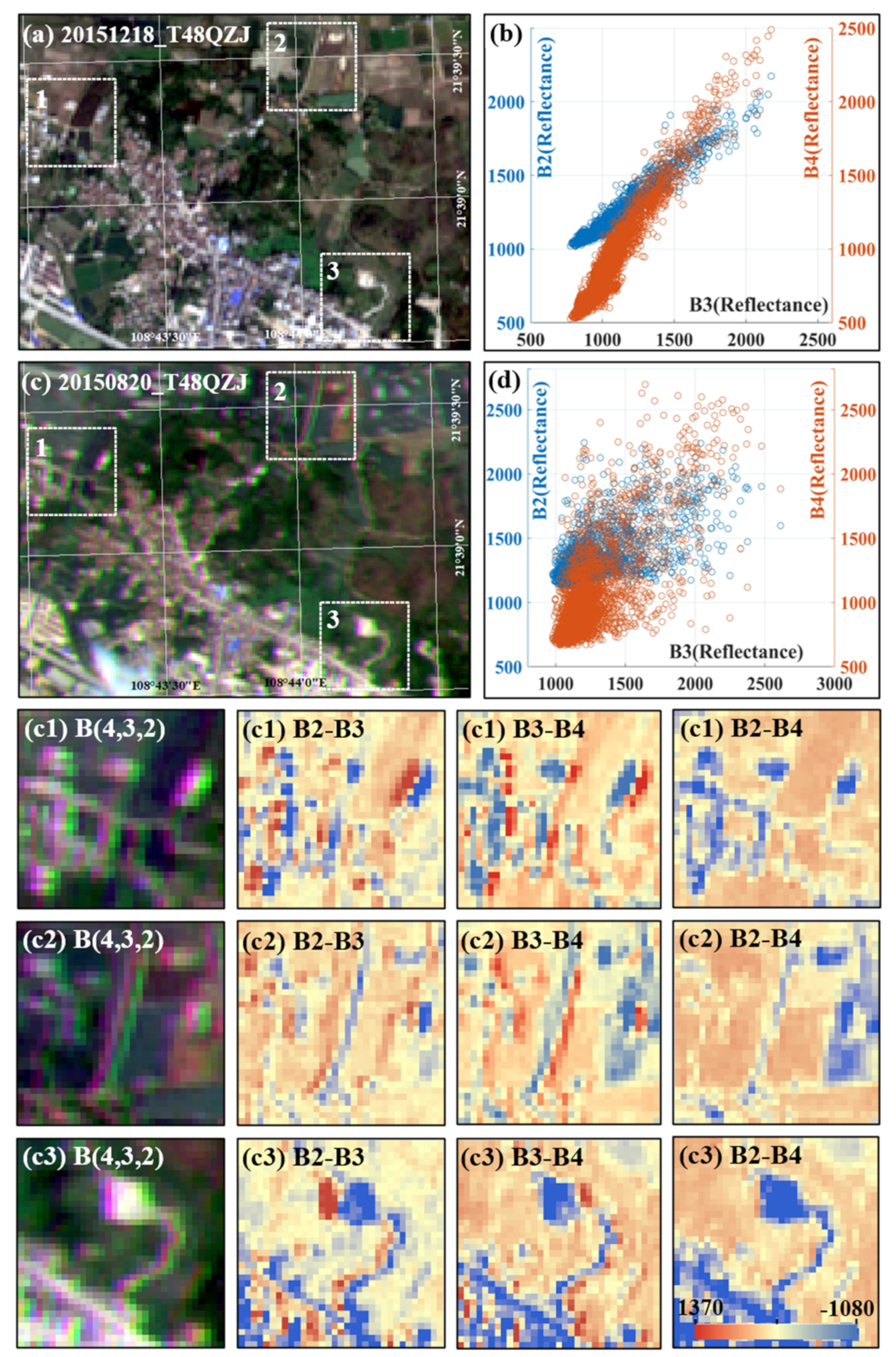
In MSI true-color images (TCI, R: Band 4; G: Band 3; B: Band 2, 10 m resolution), an inter-band displacement over one pixel can be discernable, creating a “rainbow” effect [18]. This usually comprises a bright-green stripe on one side of the geo-feature’s edge and a magenta stripe on the other side (Figure 1c). The parallax can be useful in some cases; for example, the “rainbow” effect of objects moving at high speed caused by inter-band parallax can be used to capture small targets such as vehicles, ships, and planes in high-spatial-resolution images. It can also track the motion of moving clouds and water [19,20]. Meanwhile, the blurring of object boundaries may lead to geometric deviations in target recognition or land-cover misclassifications, which affect the reliability of RS applications. As shown in Figure 1c1–c3, the green stripes show relatively high values in the differences between Bands 3 and 4, whereas the magenta stripes appear to show relatively low values. This indicates the existence of an offset between Bands 3 and 4. The offset between Bands 2 and 3 can also be observed in the same way. However, the difference between Bands 2 and 4 only displays the features of geo-objects, rather than the “rainbow” stripe, which implies there are no apparent offsets between them. According to the analysis, the displacement of Band 3 is, therefore, the leading cause of the “rainbow” effect.
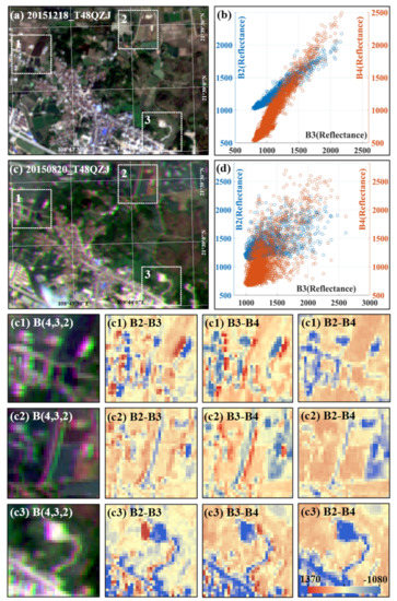
Figure 1.
MSI images with and without discernible BBMR in the visible bands (Bands 2–4). (a) A subset of an MSI true-color image (48QZJ) acquired on 18 December 2015, without BBMR; (c) a subset of an MSI true-color image acquired on 20 August 2015, with BBMR in the same area as (a); and (b–d) the correlation between the reflectance of Bands 2–3 and Bands 4–3 inside three square image chips in (a–c). (Note that the reflectance values in (b,d) were scaled by 10,000.) (c1–c3) The true-color image and difference value between the visible bands of the three chips.
Comparing MSI images with and without BBMR over the same area, we found that the relationships among the visible bands differed significantly (Figure 1a–d). Figure 1b clearly shows a higher correlation among the visible bands’ reflectance compared to that in the image without BBMR. This suggested that the inter-band offset could be captured by the bright-color feature (i.e., bright green: ρB3 − ρB2 > 0.05 and ρB3 − ρB4 > 0.05 in most images, ρ stands for the reflectance value) and could be determined by the high correlation between the visible bands. The following method was therefore proposed based on this core idea. Note that this study only focuses on the offset between the green band and the other two visible bands.
2.2. Inter-Band Mis-Registration Detection Method
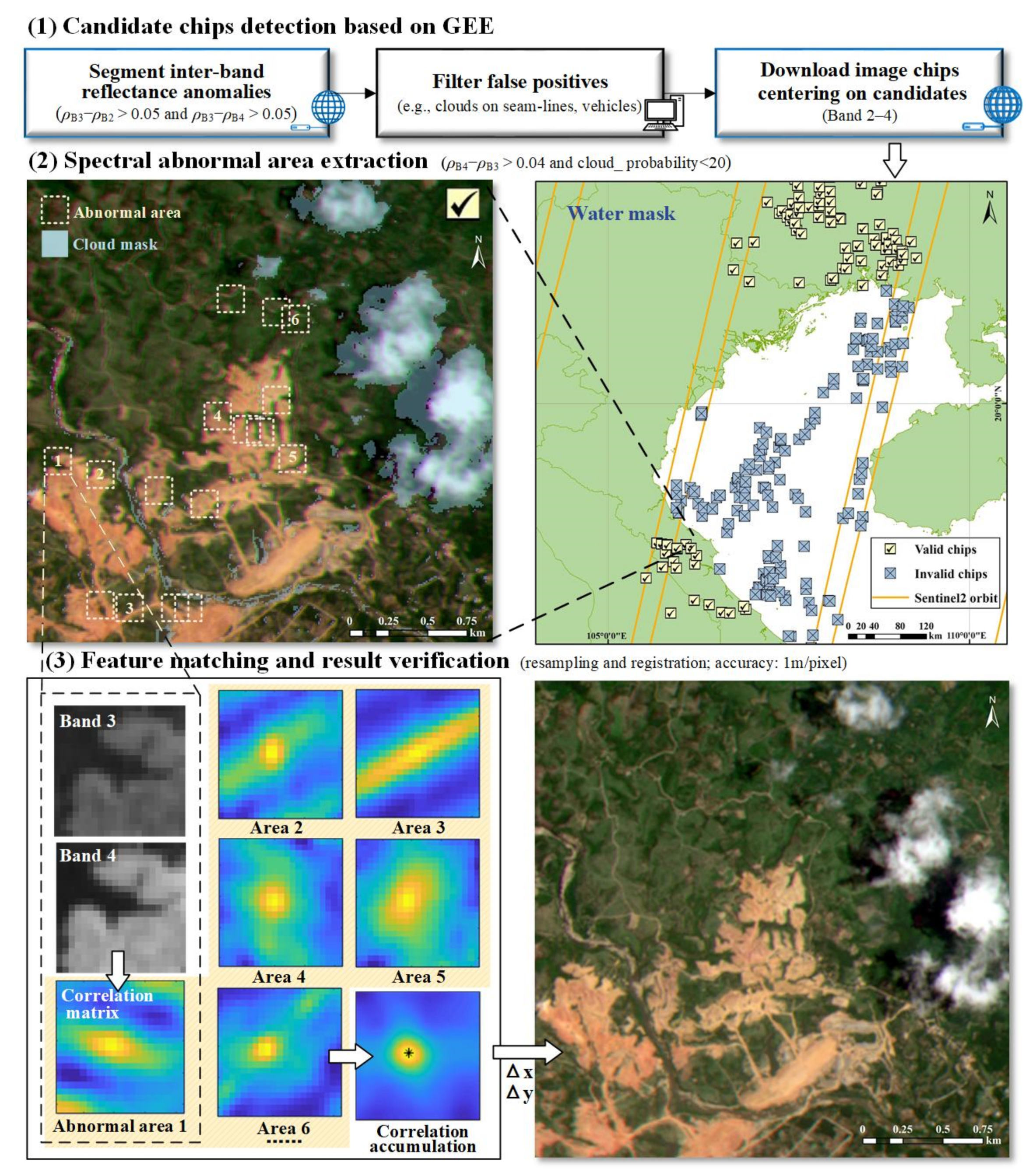
There are two types of most commonly used methods for BBMR detection: sensor based and feature based. The former focuses on building a mathematical model between the interference factors during imaging and the inter-band offset, such as reproducing the imaging process in a laboratory to calibrate the interior of the camera and relative orientation parameters [17]. The latter analyzes the spectral features of images, mostly based on the cross-correlations between bands [21,22] and processed with phase correlation or the quantile matching method [23]. The detailed procedure varies depending on the method used to locate feature points. For example, image processing methods such as quad-tree decomposition [24] and singular value decomposition [25] have been used to calculate the BBMR inside an image chip. Meanwhile, other methods have been used to select the region of interest based on entropy [26] or to construct triangulation methods [27]. For the optimal results of band-to-band registration, height difference displacement analysis [28], cloud masks, and low-rank analysis [29] have been used to provide different levels of strategies for registration. The methods mentioned above mostly targeted charge-coupled devices (CCDs) and some sensors carried on an unmanned aerial system (UAS). Note that there are few BBMR detection methods for MSI images, and a known one is processed with phase correlation calculation on a sliding window basis for a whole image [18]. However, to be applied to a series of spatiotemporal multi-spectral images, the BBMR detection method requires a more efficient determination strategy and a larger storage space. Moreover, the spectral characteristics of surface objects in RS images cannot be effectively expressed over a large spatial scale (~110 × 110 km2 for each scene). Therefore, filtering redundant data in the image and narrowing the size of the image participating in a single operation process are both priorities. We propose the following hybrid framework to detect the BBMR in MSI images, and it comprises three main steps (Figure 2): candidate chip detection based on GEE, spectral abnormal areas extraction, and feature matching. The first step shrinks the valid areas inside image scenes as potential targets to download, the second step precisely extracts pixels with spectral abnormal features inside every single chip, and the third step determines the best-fit coordinates in the accumulation cross-correlation matrix of all abnormal areas.

Figure 2.
The hybrid framework of BBMR detection in an MSI image chip. The valid candidate chips (301 × 301 pixels) were selected after spectral anomaly detection and water masks. With the filtration of clouds, the abnormal areas inside the chips were extracted to calculate the best-fit location in the correlation matrix between visible bands. (The sample chip used in this figure was subsetted from scene 20150810_T48QXE.).
2.2.1. Candidate Chip Detection Based on GEE
The computation priority on GEE is distributed by the geometrical range and complexity of the operation to guarantee efficiency in general, which means that it is not realistic to conduct the complete data calculation process online. Our strategy, which maximizes the advantages of the analysis functions of GEE, involves simplifying the online spectral abnormal area detection process and downloading all image chips containing valid spectral information from a whole scene as candidates for further determination in a local computation environment. This approach could narrow the size of an image to approximately one-thousandth that of the original scene and thus could significantly reduce local data storage requirements.
First, as described in Section 2.1, the abnormal spectral feature can be used to capture inter-band mis-registration candidates. In this experiment, our aim was to detect anomalies in Band 3 (i.e., ρB3 − ρB2 > 0.05 and ρB3 − ρB4 > 0.05) that presented bright-green features in true-color images. Then, a rough filtering of false reflectance anomalies in Band 3 needed to be conducted before downloading the image chips to minimize excessive network transferring. False anomalies along the seam-lines of two adjacent granules (caused by moving clouds) and those inside traffic networks (caused by moving vehicles) can be effectively excluded using a similar method to that used in a previous study [8]. The M-estimator sample and consensus method is used to find the linear-distributed candidates in every scene. Moving vehicles can be frequently observed along roads (especially along highways). Therefore, a frequency image is used to better exclude them in a time series of MSI images. Moreover, the sun-glint noise that appears on water surfaces with high reflectance or moving ships may also lead to false detections. Here, we use a global water map provided by the Environmental Systems Research Institute (ESRI) to filter chips that are fully covered by water surfaces as invalid data. After filtering the false positives, the detected abnormal spectral pixels are divided into different areas according to connectivity. The centroids of every area are calculated and saved as candidates in coordinate files. Finally, visible band chips (301 × 301 pixels) of MSI images centering on each candidate (pixel) with a 150-pixel extension in 4 neighborhoods could then be downloaded from the Sentinel-2 Collection on GEE.
2.2.2. Spectral Abnormal Area Extraction
The abnormal area detection methods used in image registration can be divided into two main types: area based and feature based. To obtain a more solid result while also reducing algorithm complexity, we chose the latter to locate the inter-band mis-registration points inside the chip, depending on the spectral difference between bands. The specific steps are as follows:
- (i)
- Spectral feature extraction. Inside each image chip, the threshold of the abnormal spectral point needs to be expanded to extract more features in areas with relatively low heterogeneity. The spectral reflectance peak around the green light band that vegetation has may lead to false positives if we simply narrow the threshold using the same criterion as that applied during the detection of candidate chips. Instead, we focus on bright-magenta features (ρB4 − ρB3 > 0.04) that appear in pairs with green ones in order to avoid vegetation interference. Only focusing on the BBR of the surface objects in the experiment, the “rainbow” effect appearing at the edge of moving clouds also needs to be excluded to obtain more convincing candidate points. Our primary choice of cloud mask is the cloud probability product (10 m resolution) processed by the s2cloudless open-source algorithm on GEE, because it ensures data coverage, avoids image resampling, and has significant high confidence compared to Band QA60. In this experiment, points with cloud probability of >20% were removed from the candidates. Note that the thresholds were the optimal choices determined by trial-and-error analysis and succeeded in extracting reflectance anomalies in Band 3 of MSI images covering different backgrounds. Although the performance was supported by the experiment result, the transfer to other datasets may still need more tests for adjustment.
- (ii)
- A random sampling of abnormal spectral points. If the number of candidate points inside a chip is less than three, it will be filtered as an accidental error or a flying airplane; if the number is more than 24, the chip will be divided into a 3 × 4 grid for random sampling inside each grid in order to obtain a roughly geometrical uniform distribution of 24 points inside the chip. As the chips are downloaded centering on every abnormal area, we considered that the potential mis-registration inside a chip is spatial continuous in most cases. Therefore, this shrinks the computation complexity, while maintaining the main spectral feature.
2.2.3. Feature Matching and Result Verification
The high relativity among visible bands makes it possible to assess inter-band mis-registration by cross-correlation. In this case, we only evaluate the correlation between Bands 3 and 4 because as the bright-green and red stripes appear symmetrically, the existing offset patterns between Bands 3–4 and Bands 3–2 in the experimental images are essentially the same. With each abnormal spectral point, a small window (21 × 21 pixels) is built to calculate the statistical best-fit position between Bands 3 and 4. The window is centered on the abnormal spectral pixel with a 10-pixel extension in 4 neighborhoods. The window size is designed to meet the demand of surface feature representation and reduce the number of pixels participating in every single operation at the same time. Taking the Band 3 window as the reference image and moving the Band 4 window as the sensed image in the range of 10 × 10 pixels, the image correlation is calculated at every position to establish a 21 × 21 cross-correlation matrix. This matrix is resampled into 105 × 105, and the maximum correlation value position is calculated as the best-fit position at the improved accuracy of 0.2 pixels. To enhance the abnormal spectral feature detected in different areas and reduce the error caused by object texture, we accumulate all of the cross-correlation matrices and obtain a general best-fit position of all of the candidate windows. Meanwhile, we use a k-means clustering result of all the best-fit positions to ensure reliability, because based on the assumption that the inter-band offsets are similar inside the chip, the offset at each point should also have a similar direction. If the accumulation position and the clustering position are both outside of the 0.37 × 0.37 window, with a distance within 0.75 pixels between each position, then this image chip will be considered with inter-band mis-registration. For the mis-registration result, all three bands are resampled to 0.1 pixels and Band 3 is moved back to the best-fit position for manual visual inspection to check the result. The improvement in the true-color image composition is used to verify the effect.
3. Results
3.1. Detection Results
The proposed method was applied to 71,493 scenes of MSI Level-1C top of atmosphere (TOA) reflectance images covering China and its surrounding areas (58°43′37″N–0°23′15″S, 142°29′40″E–67°8′44″E) acquired from 21 July 2015 to 28 February 2016, the first few months after the launch of Sentinel-2A. We use the candidate chip products provided by a former study into airplane detection [8], as the detection method for this experiment shares similarities in spectral features with the flying airplane detection method based on the parallax between MSI visible bands. After the reflectance anomaly detection and false-positive filter, a total of 130,784 MSI image chips from 19,842 scenes were downloaded from GEE. In the local environment, 4356 chips from 442 scenes were detected with BBMR. From this, 4272 chips from 391 scenes were confirmed with existing mis-registration by manual visual inspection with an accuracy up to 98.07% at the chip scale and 88.46% at the scene scale. The average number of downloaded chips per image was 6.59, and it only accounted for 0.49% of the total pixels in an image. The reduction of downloaded images significantly improved the computation performance. According to the test statistic of 15,388 chips from 25 July 2015 to 15 August 2015, the average operation time for a chip was 0.76 s. Therefore, the method could be considered efficient for application on a sizeable set of image data. However, the limitation of the dataset brings possibilities of more chips with BBMR that may have remained undetected, because some areas with clustered abnormal points were filtered before being downloaded. Thus, this result only presents the temporal and spatial distribution of images with BBMR to a certain extent.
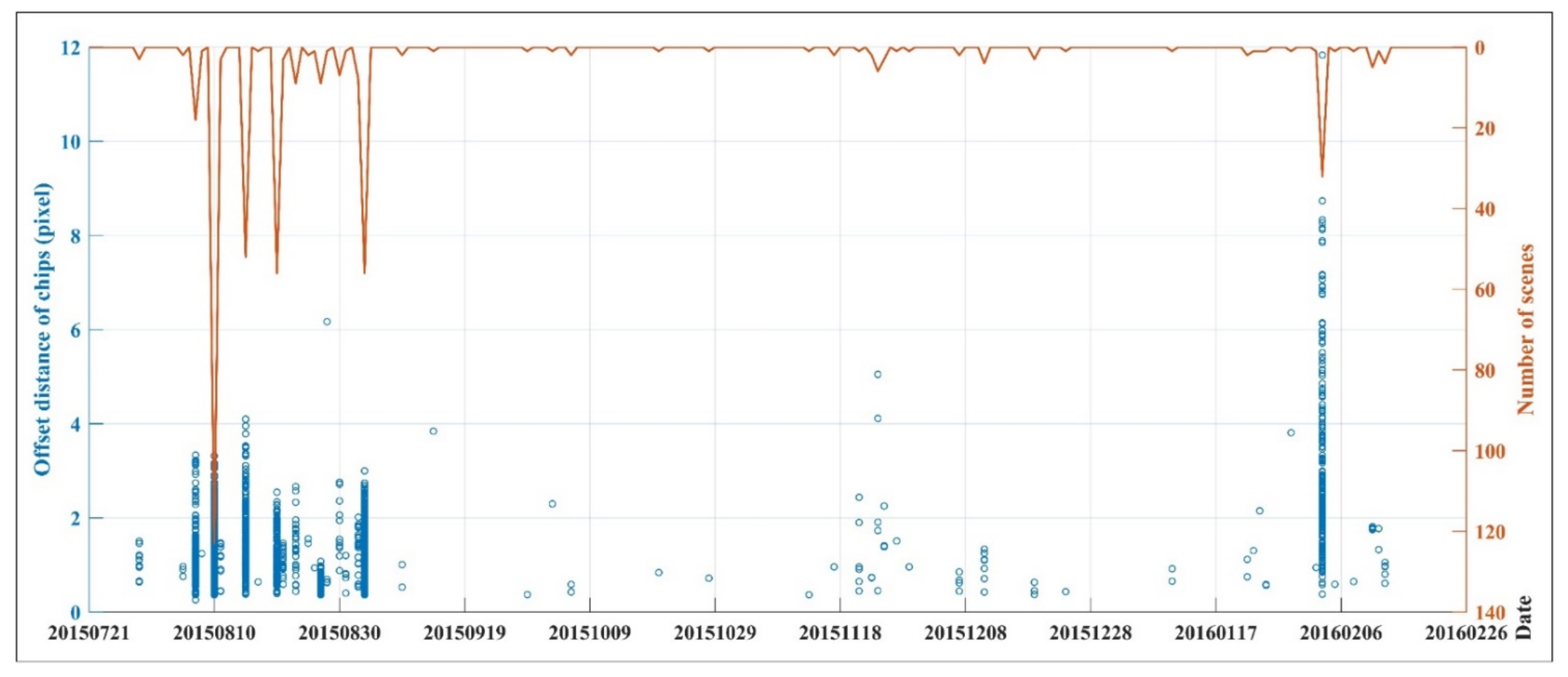
As shown in Figure 3, the chips with confirmed BBMR mainly appeared across 12 days from 29 July to 3 September 2015, during the early period following the launch of Sentinel-2A. Later in the study interval, BBMR only showed up occasionally on four days (24 November, 25 November, 11 December 2015, and 3 February 2016), and other detection results were mostly determined as false positives (53 chips from 41 scenes in 27 days). The confirmed mis-registrations not only showed up in multiple chips inside a single day but often in multiple scenes as well. The peak appeared on 10 August 2015, when there were 1431 chips with BBMR captured from 123 scenes, followed by 20 August and 3 September 2015 with 56 scenes and 15 August 2015 with 52 scenes. Although there was no apparent temporal pattern regarding the repetitive spatial appearances of BBMR, they did occur on some of the scenes over several days: scenes T50TML, T50TLL, and T50TLK were each detected to have BBMR four times, with 9 scenes detected three times and 40 scenes detected twice. Most offset distances were in the range of 0.37–3, with 77.40% of chips under 1.5 pixels, 90.67% of chips under 2.0 pixels, and 95.25% of chips under 2.5 pixels. The proportion of these images is not quite high due to the fine quality of the Sentinel-2 product; hence mis-registration could be an easily neglected problem. Therefore, we believe this method is essential and necessary for further remote sensing applications.
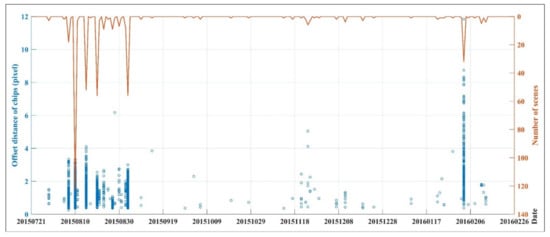
Figure 3.
Temporal distribution of chips and scenes with an inter-band offset. The chips are represented with blue circles by the offset distance (pixel); the orange line represents the trend of scenes.
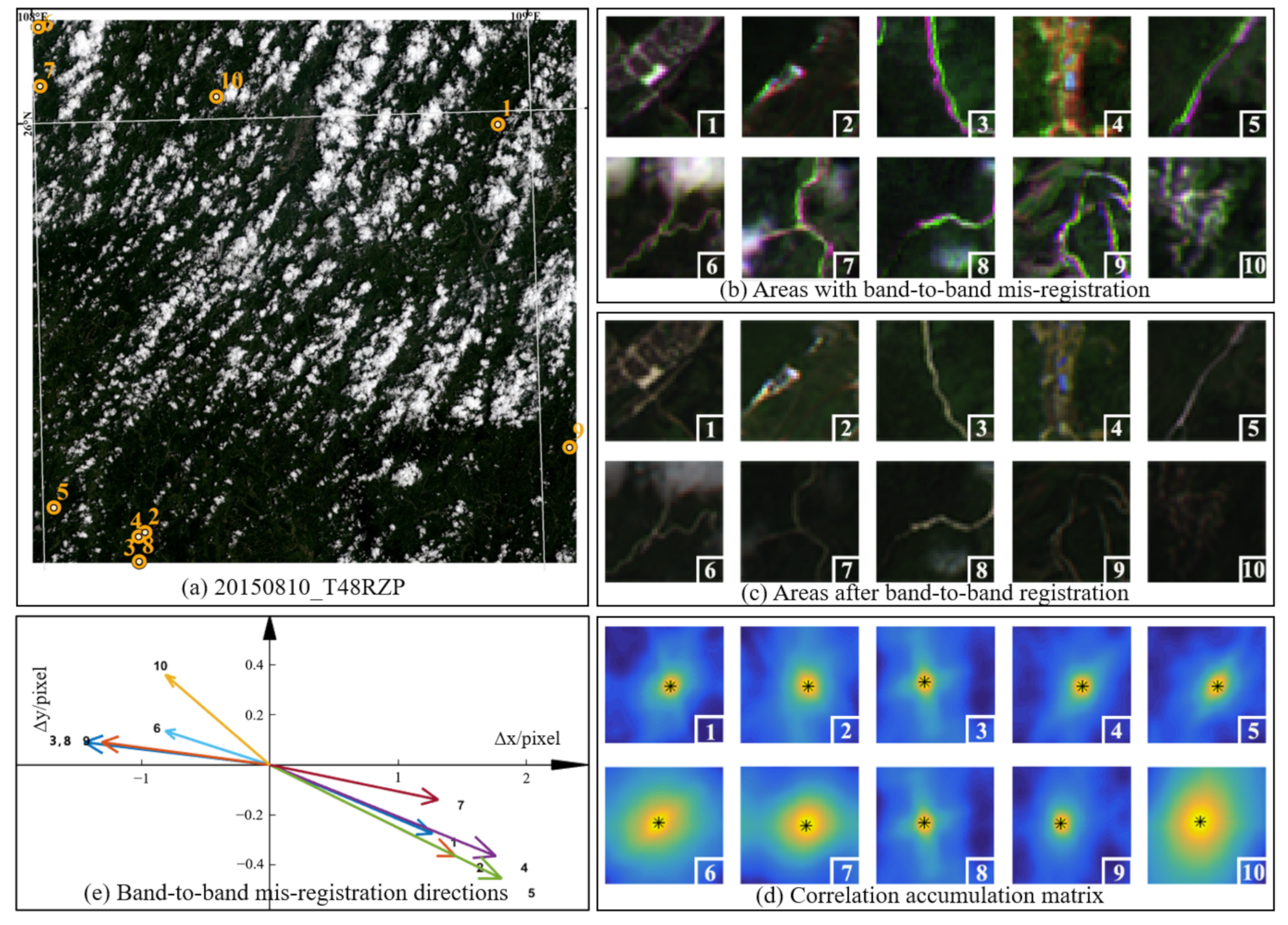
The BBMR distances and directions not only varied between different chips acquired on the same day (Figure 3) but also varied between different chips inside the same scene. For example, 10 chips detected to have confirmed BBMR (Figure 4b) in scene 20150810_T48RZP showed different offset distances and directions (Figure 4e) without representing a distinct spatial clustering pattern. This indicates that the offset was not homogeneous inside the range of the scene. Therefore, images need to be defined into smaller units for more precise BBMR detection and correction. In this research, we only focused on quick BBMR detection. The discontinuity between different chips will not affect the reliability of the result, because the detection will not accurately extract the boundary of the mis-registration area. However, based on the detection result, the requirement of fine registration for further application may need a continuous area border. The other method mentioned in Section 4.3 may provide a potential support to solve this problem with a flexible window.
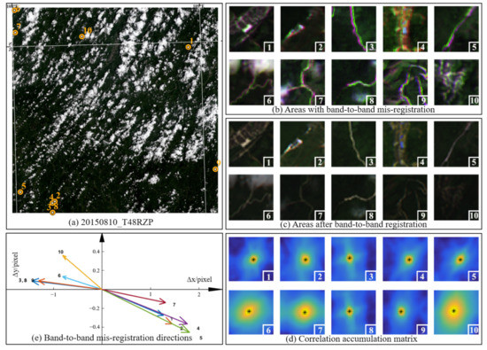
Figure 4.
Inter-band offset directions and distances of different chips inside one scene. (a) Positions of 10 chips in scene 20150810_T48RZP, (b) original true-color images of these chips, (c) BBR results of these chips, and (d,e) different offset directions and distances of these chips. Note that image chips in (b,c) were zoomed in (40 × 40 pixels) to better present the spectral feature.
To analyze the performance of this method, a test area from scene T48PYC (10,000 × 10,000 m2, centered on 15.5157°N, 107.8083°S) was tracked from 21 July 2015 to 28 February 2016 with manual visual inspection to check the detection result. From 45 scenes acquired from 18 days during this period (including all versions of images with different processing dates), the image acquired on 20 August 2015, processed on 26 April 2016, was detected and confirmed with BBMR. In the rest of the negative images, 24 were confirmed without BBMR and 20 were fully covered by clouds. This could support the reliability of the proposed method with a low probability of mis-detection.
3.2. Spatial Distribution of Detected MSI Chips with BBMR
To better analyze the spatial distribution of the detection results, all of the geographical positions were plotted on a map in Figure 5a. The images acquired on 10 August, 20 August, 23 August, 27 August, and 3 September 2015 appeared in two relative orbits across mid-eastern China, making up the main clustering area. The detections from other days showed up sporadically in other areas. Furthermore, the inter-band offset distance did not show a clear spatial pattern related to the trajectory of the satellite or to the geographical location of the image. To further analyze the inter-band offset direction pattern, a rectangular coordinate was established, as shown in Figure 5b. Based on the random sample consensus algorithm, we constructed a fitting straight line through the origin (y = −0.1784x) to represent the general trend of the clustering offsets in the second and fourth quadrants; 96.06% of offsets were inside the boundary of an ellipse centering on the origin with the same orientation angle as this fitting line (major axis: 8, minor axis: 2). The spatial distribution of the inter-band offset directions along the fitting line shows a possible connection between the offset direction and the orbital motion direction of the satellite, because the angle between the minor axis of the ellipse and x-axis (100.11°) is close to the orbit inclination of Sentinel-2A (98.62°).
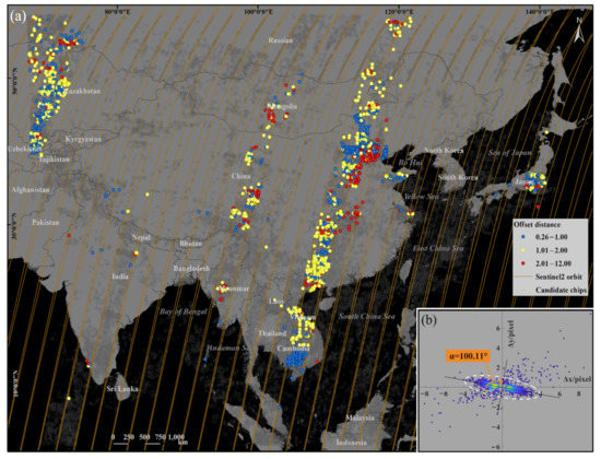
Figure 5.
Spatial distribution of image chips with detectable BBMR. (a) Distribution of chips around China and its neighboring areas. The chips detected with BBMR were graded by the offset distance with different colors, and other candidate chips were represented by gray circles. (b) Sets the offset position of 4356 detected chips to a rectangular coordinate with a fitting ellipse (covered 96.06% chips) centered on the origin.
4. Discussion
4.1. Limitations
4.1.1. Limitations of Introducing Additional Data
Noticeable spectral differences between visible bands can be widely observed near objects with high reflectivity features, such as water surfaces or clouds, leading to a large amount of false detection. Due to the limitation of spectral features provided by visible bands, it is challenging to filter this kind of error solely by analyzing the texture features of each chip. Therefore, we introduced additional data into the experiment to create both water masks and cloud masks to reduce these particular false detections. However, the practical data and method both still have some flaws.
- (i)
- Cloud masks. The machine-learning-based cloud detection product achieves much higher accuracy in cloud filtering than Band QA60 (Figure 6b,c). In some cases, however (Figure 6(b3)), it might show a false high probability in areas without clouds. This could lead to the omission of some significant abnormal spectral points, which in turn may affect the BBR accuracy. To guarantee the filtration of clouds in most chips, the threshold of the cloud probability cannot be set too low. Thus, we adjusted the threshold while eroding the edge of the logical operation matrix to lessen the mis-filtering of ground objects. For comparison, we used chips acquired on 15 August, 20 August (with multiple confirmed BBMRs), and 1 December 2015 (without BBMRs) as experimental data to test the effect of introducing the s2cloudless product (Table 1). While a few mis-detections appeared on 15 August and 20 August 2015, the number of false detections increased significantly, leading to a significant drop in accuracy from ~90% to ~40%. Meanwhile, all of the newly added detections were confirmed as false positives on 1 December 2015. This indicates that introducing a cloud mask leads to some mis-detections on days when images with known BBMR appear. However, in most cases (especially on days without confirmed BBMR images), the increment in detection accuracy was notable. Considering that BBMR is known to occur regularly (it tends to appear in multiple chips and scenes inside one day), missed detections will not greatly affect the general temporal tendency compared to the significant number of false positives that would be detected without the cloud mask. The crucial role that the mask plays in the filtration of moving clouds cannot currently be substituted. Thus, we regard this error as acceptable in the context of our experiment.
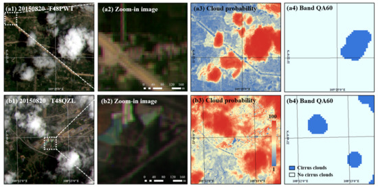 Figure 6. Influence of detection results with the introduction of cloud masks. (a1–b4) Compares the accuracy of the s2cloudless product and Band QA60 in two scenes with BBMR. The s2cloudless product identifies the range of the cloud more precisely than Band QA60 in most cases like (a3,a4), but sometimes also presents a false high value in areas like (b3), leading to the mis-detection of BBMR.
 Table 1. Influence of introducing a cloud mask on detection results.
- (ii)
- Water masks. Although the movements of seam-lines and the edges of lakes and rivers did not represent notable differences in kilometer-scale TOA images, the global water map still could not filter all of the chips that were capturing water surfaces, as there were some inevitable errors during the process of rasterization and the resampling of the water shapefile data; these errors may affect the accuracy of water masking. If using the Sentinel water surface classification product, additional errors may also be caused by interpretations such as the cloud mask, which may bring about new problems. According to the results, the proportion of false-positive detections caused by water was extremely low (5 of 4363 chips, 0.11%), and we consider that it is of no great significance to introduce the water surface classification product to optimize the result.
4.1.2. The Limitation of Application in Exceptional Cases
- (i)
- Homogeneous areas. The main limitation of the proposed method is that it is based on the assumption that there is sufficient variance inside each chip and that there will be a unique and clear maximum in every correlation matrix, corresponding to the offsets between bands. However, areas such as deserts and grasslands, which have repetitive or almost homogeneous textures may have a rather low variance in a small image chip. This homogeneity could lead to an inaccurate offset direction. In our experiment, there were few image chips in which we could not distinguish the difference before and after BBR visually, due to a lack of discernable features outstanding from the image background. This indicates that the accumulation correlation matrix can mitigate the influence of homogeneous areas in most cases, and the false-positive results that arise occasionally will only have a slight impact on the detection accuracy.
- (ii)
- Areas with complex inter-band offsets. Our method assumes that the feature of mis-registration between bands shows spatial consistency within the scale of one chip (301 × 301 pixels). However, the situation is much more complicated in practical terms. We found out that in some chips, both the range and the spatial features of the mis-registration could not fit the previously expected ideal state. These kinds of cases often show up in areas with obvious topographic relief in the experiment images. As shown in Figure 7a, although mis-registration was successfully detected and corrected in part of the chip (Figure 7(a2)), some areas (Figure 7(a1)) without visual errors showed new mis-registrations after registration. Segmenting chips into smaller regions or re-performing a spectral anomaly detection on the image after BBR may filter this kind of error.
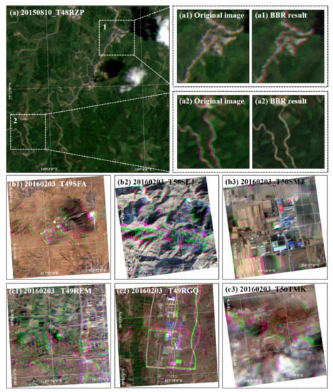 Figure 7. Examples of areas with complex inter-band offset. (a) The inter-band offset only appeared in part of the chip of 20150810_T48RZP, and the BBR of (a2) leads to a new error in (a1). (b1–c3) Some complex offset acquired on 3 February 2016; the offset in (b1–b3) can be detected, but the registration effect is limited; the offset in (c1–c3) cannot be detected.
In few cases, mis-registration can become dramatically complicated (Figure 7b,c): chips represent more than two types of inter-band offset errors, including translation, rotation, and mirror symmetry, and offsets can sometimes occur between three bands at the same time (Figure 7(b2),(c2)). Due to the spatial and spectral limitation of this method, although some chips can be captured (Figure 7(b1)–(b3)), a small number of chips still cannot be effectively detected (Figure 7c1–(c3)). These cases indicate that rigid registration methods, such as the simple translation provided, cannot fix complicated instances of BBMR within the scale of the chip. This demonstrates the need for better BBR strategies to apply to broader contexts. Nonetheless, this kind of rare abnormal situation only occurred on one day during our experiment. Therefore, considering the primary purpose of identifying mis-registrations, we consider it to be an accidental situation.
4.1.3. Limitations of the Image Dataset
The method for capturing candidate chips shares similarities in spectral features with a previously published airplane detection method based on the parallax between MSI visible bands [8]; the latter differs in that it focuses more on the separate single target. Actually, many BBMRs observed in the image chips during the parallax research inspired us to propose a method to trace the inter-band mis-registration over time. GEE keeps updating image data with more accurate registration results, meaning that much fewer inter-band offsets could be observed in the images that were re-downloaded in 2019 for the purposes of this study. Thus, considering the unity and integrity of the original features, we decided to use the existing data products downloaded from 21 May 2019 to 27 June 2019 for this experiment. The limitations of the experimental image dataset may therefore have caused some mis-detections due to filtering of the clustered spectral abnormal area. However, the detection result could still be valuable as a reference to reveal the general tendency of MSI BBR accuracy development during the early period following the launch of Sentinel-2A.
4.2. Transferability to Other MSI Bands
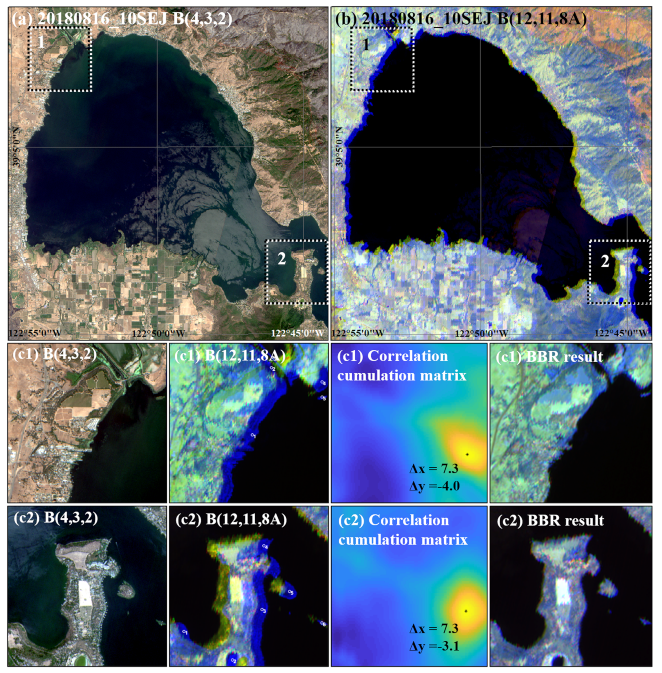
The MSI visible bands were used in this experiment, but the core of this method could be applied to other MSI bands or satellite data based on GEE. Taking Bands 8A (NIR), 11 (near-SWIR), and 12 (far-SWIR) of the MSI images as an example, in scene 20180816_T10SEJ, the true-color image did not represent an apparent inter-band offset among the visible bands (Figure 8a). However, in a false-color image (R: 12, G: 11, B: 8A) with 20 m spatial resolution, there was a nearly 11-pixel dislocation around the edge of the lake (Figure 8b). These bands could be used to build a spectral thermal anomaly index to detect high-temperature thermal anomalies. Therefore, the inter-band mis-registration may have led to many false positives during thermal anomaly detection and could have introduced unreliability in subsequent work. This dislocation was determined to appear between Band 8A and the other bands, following difference analysis among the three bands. By performing a procedure similar to that carried out during BBMR detection for visible bands, the anomaly pixels in this scene could also be captured by a particular feature (ρB8A > 0.21, ρB12 < 0.01, ρB11 < 0.01) and ameliorated to a certain extent, as shown in Figure 8(c1),(c2).

Figure 8.
Apparent BBMR exists among MSI Band 8A and SWIR bands (Bands 11 and 12), while there is hardly discernible BBMR among visible bands (Band 2–4) of the same acquisition. (a) A subset of true-color MSI image (10SEJ) acquired on 16 August 2018, (b) false-color image (Bands 8A, 11, and 12) of the same extent as (a), and (c1,c2) examples of a rough BBR process in two image chips (Bands 12, 11, 8A; size: 168 × 168 pixels) cut from scene 10SEJ.
Due to the complexities of the spectral features in these bands, the establishment of a generally applicable extraction method for anomalies requires further research. Similarly, the abnormal spectrum area can also be captured by the spectrum differences between other target bands, while discriminant conditions might be more complicated depending on their inter-band spectrum covariance. Thus, the method proposed here might exhibit a certain generality and superiority regarding the detection of long-term inter-band mis-registration.
4.3. Comparison with Existed BBMR Detection Method
In comparison to another existed BBMR detection method promoted by Skakun et al. (2017) [18] for MSI images, the main improvement in this paper is the change in calculation objects. Differentiating from a calculation traversing the whole image, the method promoted in this paper is target originated, which considerably reduces the number of pixels that participate in the operation.
The method promoted by Skakun et al. was based on the phase correlation calculation on a sliding window basis. With the adjustment of window size and step length, this method could be applied to detect moving targets such as planes or clouds. However, this paper is focused on the BBMR detection of static objects, which fail to meet the required threshold of multispectral band registration. Therefore, moving targets such as airplanes, ships, and clouds need to be eliminated from detecting objects. The potential application of Skakun et al.’s method does not quite match our needs. In this case, the sliding window is more suitable for further spatial analyzation of BBMR in a detected area to refine the result. For example, in some cases, the BBMR did not show spatial consistency within the scale of one chip (301 × 301 pixels), as we discussed in Section 4.1, and therefore, a fine boundary of BBMR area is needed to avoid the occurrence of new mis-registration in other areas after the correction. It could also be used in areas with complex BBMR to determine different directions of offsets between bands in the adjacent parts inside an image chip. Moreover, this method may also have potential application in the analysis for spatially continuously changing events such as cloud motion or hydrological events.
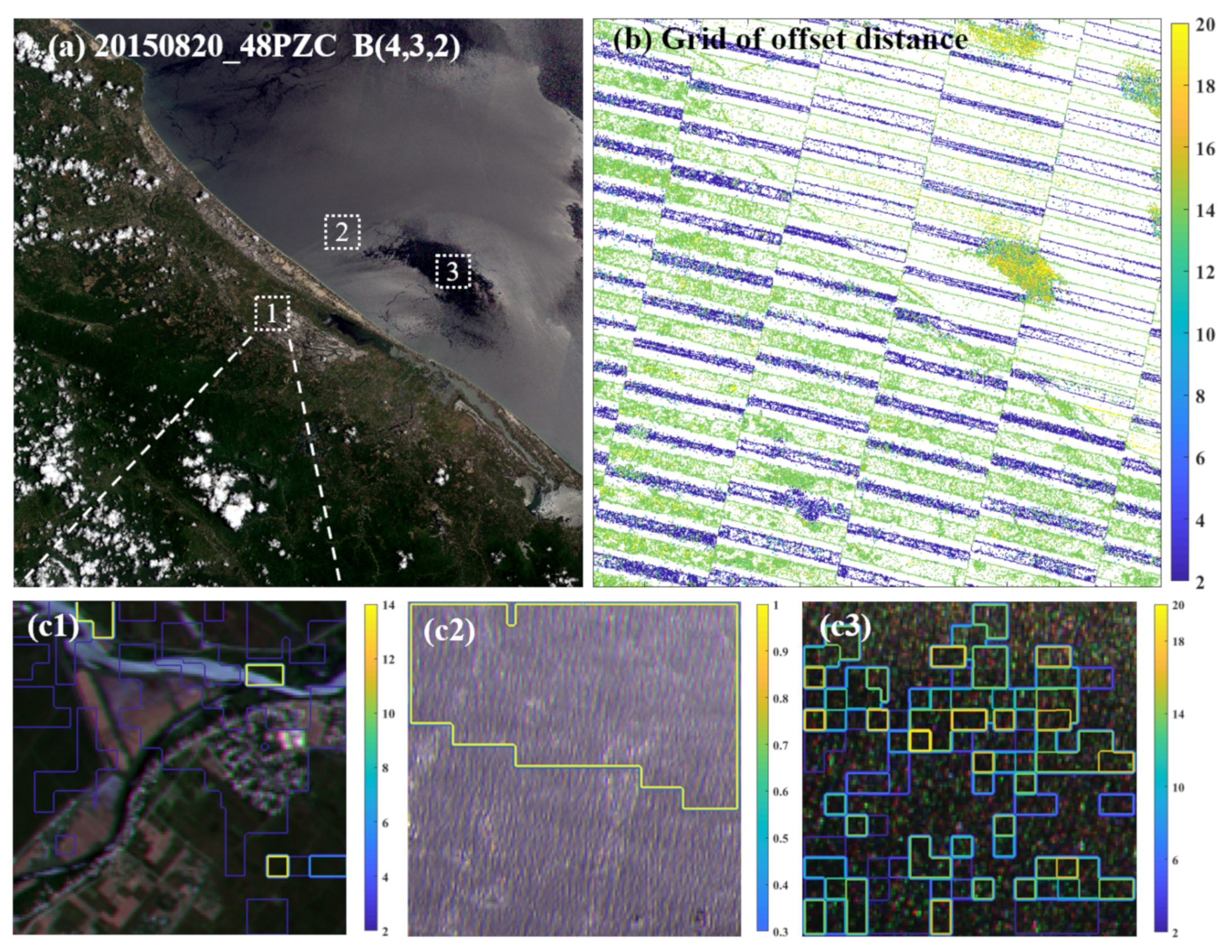
As shown in Figure 9, scene 20150820_48PZC (processed on 26 April 2016) was detected with serious BBMR. The mis-registration areas were widely distributed inside this image. We used a sliding window basis (window size: 16 × 16 pixels, step length: 9 pixels) for BBMR detection, and the result is shown as a contour (Figure 9b). Targeting the detection of the BBMR area, the result is effective on land (Figure 9c1) but still has trouble filtering the water surface with sun-glint (Figure 9c2) or other noise (Figure 9c3). Moreover, in many other images, BBMR only showed up in the local area with a small proportion of pixels. Therefore, if we use a sliding window to scan the whole image, the invalid calculation times will tremendously increase in each determination process. Although the efficiency can be improved by the adjustment of the size and step length of a sliding window, it still requires considerable operations to acquire a subpixel level offset result. With the introduction of a pre-processing procedure to cut the original image into chips, the method promoted in this paper diminishes the image data involved in the calculation. The conditional random sampling step to choose feature points inside each image chip makes a further data reduction.
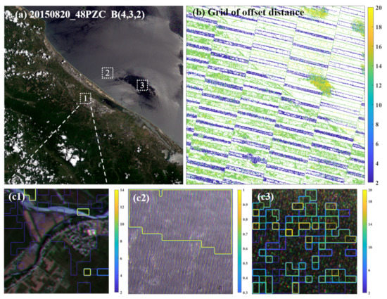
Figure 9.
A true-color image with BBMR and the detection result using the phase correlation calculation on a sliding window basis (window size: 16 × 16 pixels, step length: 9 pixels). The result is presented as a grid with a colored border, divided by the inter-band offset distance (pixels) in (b). (c1–c3) The zoom-in image clips (150 × 150 pixels) from the marked areas in the image (a) with a contour result overlay.
To summarize, the method promoted in this paper is more suitable for quick BBMR detection in a large number of images due to the improved computing model based on chips. The existed BBMR method could acquire a more accurate BBMR boundary, and it could be applied to optimize our results in some cases.
5. Conclusions
The recent development of cloud sharing and computing technology has made it easier for researchers to access massive amounts of geographic image data. Though this provides convenience, it also brings higher demands on retrieval methods and data quality to ensure the reliability and efficiency of further applications. As for MSI images, determining unqualified image with band-to-band mis-registration is crucial for subsequent RS application. It is more challenging because time efficiency and the elimination of redundant information both need to be carefully considered to handle the ever-increasing MSI images. Here, we proposed a hybrid framework for detecting BBMR between the visible bands in MSI images, including rough GEE online pre-processing and a precise local operation. To enhance the efficiency of handling massive MSI images, we adopted online feature filtration to extract spectral abnormal areas in the MSI images, potentially caused by the band-to-band mis-registration; and to guarantee the robustness, we conducted band correlation to determine the presence of BBMR, only based on image chips containing spectral abnormal areas derived from the online operation.
The proposed BBMR detection framework was applied to 71,493 scenes, and the results were used to reproduce the spatial and temporal distributions of images with BBMR during a seven-month period at both chip and scene scales. Although limitations remained, leading to some mis-detections, the results were still able to reveal trends in BBR accuracy during the early period after the launch of Sentinel-2A. The hybrid computation framework proposed here may also be transferable to BBMR detection in other bands or with other satellite data. This process would demand the adjustment of spatial features and the optimization of the geometry registration to address more complicated situations. Moreover, by combining both online and local computation advantages, this method provides an efficient perspective for users to conveniently evaluate image quality when dealing with a large amount of data. This idea may have further potential applications in other image-processing problems.
Author Contributions
Conceptualization, T.C. and Y.L.; methodology, resources, investigation, writing—review and editing, supervision, Y.L.; software, writing—original draft preparation, visualization, T.C. All authors have read and agreed to the published version of the manuscript.
Funding
This research was supported by the Key Research and Development Program of China (grant no. 2019YFA0606601) and the Jiangsu Provincial Natural Science Foundation (grant no. BK20160023).
Data Availability Statement
The authors are grateful to the European Space Agency (ESA) and Google Earth Engine (GEE) for providing Sentinel-2 MSI images and online computation.
Conflicts of Interest
The authors declare no conflict of interest.
References
- Fang, Z.; Cao, C.; Jiang, W.; Ji, W.; Xu, M.; Lu, S. Multi-Spectral Image Inter-Band Registration Technology Research. In Proceedings of the 2012 IEEE International Geoscience and Remote Sensing Symposium, Munich, Germany, 22–27 July 2012; pp. 4287–4290. [Google Scholar]
- Xie, Y.; Xiong, X.; Qu, J.J.; Che, N.; Wang, L. Sensitivity analysis of MODIS band-to-band registration characterization and its impact on the science data products. SPIE Opt. Eng. Appl. 2007, 6679, 667908. [Google Scholar]
- Xu, H.; Sun, R.; Zhang, L.; Tang, Y.; Liu, S.; Wang, Z. Influence on Image Interpretation of Band to Band Registration Error in High Resolution Satellite Remote Sensing Imagery. In Proceedings of the 2012 2nd International Conference on Remote Sensing, Environment and Transportation Engineering, Nanjing, China, 1–3 June 2012; pp. 1–4. [Google Scholar]
- Belward, A.S.; Skoien, J.O. Who launched what, when and why; trends in global land-cover observation capacity from civilian earth observation satellites. ISPRS J. Photogram. Remote Sens. 2015, 103, 115–128. [Google Scholar] [CrossRef]
- ESA. Sentinel-2 User Handbook. Available online: https://sentinel.esa.int/documents/247904/685211/Sentinel-2_User_Handbook (accessed on 24 April 2020).
- ESA. Sentinel-2 Technical Guides. Available online: https://earth.esa.int/web/sentinel/technicalguides/sentinel-2-msi/performance (accessed on 24 April 2020).
- Gascon, F.; Bouzinac, C.; Thépaut, O.; Jung, M.; Francesconi, B.; Louis, J.; Lonjou, V.; Lafrance, B.; Massera, S.; Gaudel-Vacaresse, A.; et al. Copernicus Sentinel-2A Calibration and Products Validation Status. Remote Sens. 2017, 9, 584. [Google Scholar] [CrossRef] [Green Version]
- Liu, Y.; Xu, B.; Zhi, W.; Hu, C.; Dong, Y.; Jin, S.; Lu, Y.; Chen, T.; Xu, W.; Liu, Y.; et al. Space eye on flying aircraft: From Sentinel-2 MSI parallax to hybrid computing. Remote Sens. Environ. 2020, 246, 111867. [Google Scholar] [CrossRef]
- ESA. Sentinel-2 L1C Data Quality Report. Available online: https://sentinel.esa.int/documents/247904/685211/Sentinel-2_L1C_Data_Quality_Report/6ad66f15-48ca-4e65-b304-59ef00b7f0e0?version=1.56 (accessed on 6 February 2020).
- Berger, M.; Moreno, J.; Johannessen, J.A.; Levelt, P.F.; Hanssen, R.F. ESA’s sentinel missions in support of Earth system science. Remote Sens. Environ. 2012, 120, 84–90. [Google Scholar] [CrossRef]
- Malenovský, Z.; Rott, H.; Cihlar, J.; Schaepman, M.E.; García-Santos, G.; Fernandes, R.; Berger, M. Sentinels for science: Potential of Sentinel-1, -2, and -3 missions for scientific observations of ocean, cryosphere, and land. Remote Sens. Environ. 2012, 120, 91–101. [Google Scholar] [CrossRef]
- Hass, E.; Hill, J.; Stoffels, J.; Frantz, D.; Uhl, A. Improvement of the Fmask algorithm for Sentinel-2 images: Separating clouds from bright surfaces based on parallax effects. Remote Sen. Environ. Interdiscip. J. 2018, 215, 471–481. [Google Scholar]
- Munyati, C. The potential for integrating Sentinel 2 MSI with SPOT 5 HRG and Landsat 8 OLI imagery for monitoring semi-arid savannah woody cover. Int. J. Remote Sens. 2017, 38, 4888–4913. [Google Scholar] [CrossRef]
- Pahlevan, N.; Balasubramanian, S.V.; He, J.; Sarkar, S.; Franz, B.A. Sentinel-2 MultiSpectral Instrument (MSI) data processing for aquatic science applications: Demonstrations and validations. Remote Sen. Environ. Interdiscip. J. 2017, 201, 47–56. [Google Scholar] [CrossRef]
- ED Chaves, M.; CA Picoli, M.; D Sanches, I. Recent Applications of Landsat 8/OLI and Sentinel-2/MSI for Land Use and Land Cover Mapping: A Systematic Review. Remote Sens. 2020, 12, 3062. [Google Scholar] [CrossRef]
- ESA. Sentinel-2 Products Specification Document. Available online: https://sentinel.esa.int/documents/247904/349490/S2_MSI_Product_Specification (accessed on 24 April 2020).
- Ping, J.J.; Yeou, R.J.; Ying, H.C. Band-to-band registration and ortho-rectification of multilens/multispectral imagery: A case study of MiniMCA-12 acquired by a fixed-wing UAS. ISPRS J. Photogramm. Remote Sens. 2016, 114, 66–77. [Google Scholar]
- Sergii, S.; Eric, V.; Jean-Claude, R.; Christopher, J. Multi-spectral misregistration of Sentinel-2A images: Analysis and implications for potential applications. IEEE Geosci. Remote Sens. Lett. 2017, 14, 2408–2412. [Google Scholar]
- Amos, C.; Petropoulos, G.P.; Ferentinos, K.P. Determining the use of Sentinel-2A MSI for wildfire burning & severity detection. Int. J. Remote Sens. 2019, 40, 905–930. [Google Scholar] [CrossRef]
- Kääb, A.; Leprince, S. Motion detection using near-simultaneous satellite acquisitions. Remote Sens. Environ. 2014, 154, 164–179. [Google Scholar] [CrossRef] [Green Version]
- Berenstein, C.A.; Kanal, L.N.; Lavine, D.; Olson, E.C. A Geometric Approach to Subpixel Registration Accuracy. Comput. Graphics Image Proc. 1987, 40, 334–360. [Google Scholar] [CrossRef]
- Yang, K.; Fleig, A.J.; Electric, I.o.; Engineer, E. MODIS band-to-band registration. In Proceedings of the IGARSS 2000, IEEE 2000 International Geoscience and Remote Sensing Symposium. Taking the Pulse of the Planet: The Role of Remote Sensing in Managing the Environment. Proceedings (Cat. No.00CH37120), Honolulu, HI, USA, 24–28 July 2000; pp. 887–889. [Google Scholar]
- Kim, W.; Jung, S.; Moon, Y.; Mangum, S.C. Morphological Band Registration of Multispectral Cameras for Water Quality Analysis with Unmanned Aerial Vehicle. Remote Sens. 2020, 12, 2024. [Google Scholar] [CrossRef]
- Simper, A.; Electric, I.O.; Engineer, E. Correcting general band-to-band misregistrations. In Proceedings of the 3rd IEEE International Conference on Image Processing, Lausanne, Switzerland, 19 September 1996; pp. 597–600. [Google Scholar]
- Hao, L.; Tuanjie, L.; Haiqing, Z. High-accuracy band to band registration method for multi-spectral images of HJ-1A/B. J. Electron. 2012, 29, 361–367. [Google Scholar]
- Du, Q.; Bruce, L.M.; Orduyilmaz, A.; Raksuntorn, N. Automatic Registration and Mosaicking for Airborne Multispectral Image Sequences. Photogramm. Eng. Remote Sens. J. Am. Soc. Photogramm. 2008, 74, 169–181. [Google Scholar] [CrossRef]
- Pan, J.; Zhu, Y.; Wang, M.; Zhang, B.X. Parallel Band-to-Band Registration for HJ-1A1B CCD Images Using OpenMP. In Proceedings of the 2011 International Symposium on Image and Data Fusion, Yunnan, China, 9–11 August 2011; pp. 1–4. [Google Scholar]
- Hassanpour, M.; Javan, F.D.; Azizi, A. Band to Band Registration of Multi-Spectral Aerial Imagery—Relief Displacement and Miss-Registration Error. ISPRS Int. Arch. Photogramm. Remote Sens. Spat. Inform. Sci. 2019, XLII-4/W18, 467–474. [Google Scholar] [CrossRef] [Green Version]
- Zhao, X.; Gao, Z.; Sun, W.; Wen, F. A Coarse-To-Fine Band Registration Framework for Multi/Hyperspectral Remote Sensing Images Considering Cloud Influence. ISPRS Ann. Photogramm. Remote Sens Spat. Inform. Sci. 2020, V-3-2020, 201–208. [Google Scholar] [CrossRef]


Publisher’s Note: MDPI stays neutral with regard to jurisdictional claims in published maps and institutional affiliations. |
© 2021 by the authors. Licensee MDPI, Basel, Switzerland. This article is an open access article distributed under the terms and conditions of the Creative Commons Attribution (CC BY) license (https://creativecommons.org/licenses/by/4.0/).