Abstract
This paper provides an overview of the Dragon 4 project dealing with operational monitoring of sea ice and sea surface salinity (SSS) and new product developments for altimetry data. To improve sea ice thickness retrieval, a new method was developed to match the Cryosat-2 radar waveform. Additionally, an automated sea ice drift detection scheme was developed and tested on Sentinel-1 data, and the sea ice drifty capability of Gaofen-4 geostationary optical data was evaluated. A second topic included implementation and validation of a prototype of a Fully-Focussed SAR processor adapted for Sentinel-3 and Sentinel-6 altimeters and evaluation of its performance with Sentinel-3 data over the Yellow Sea; the assessment of sea surface height (SSH), significant wave height (SWH), and wind speed measurements using different altimeters and CFOSAT SWIM; and the fusion of SSH measurements in mapping sea level anomaly (SLA) data to detect mesoscale eddies. Thirdly, the investigations on the retrieval of SSS include simulations to analyse the performances of the Chinese payload configurations of the Interferometric Microwave Radiometer and the Microwave Imager Combined Active and Passive, SSS retrieval under rain conditions, and the combination of active and passive microwave to study extreme winds.
1. Introduction
The ocean, which covers 71% of the earth’s surface, is an important component of the global climate system. Ocean satellite monitoring (including frozen regions, i.e., sea ice) is of great significance for observing large-scale spatial and temporal changes of various ocean parameters over long periods of time and for linking them with global climate change. Furthermore, remote sensing is an important means for continuous monitoring of single ocean regions and the generation of products that provide information about, e.g., regional wind, wave, or sea ice conditions. The European EnviSat, SMOS, CryoSat-2, and Sentinel series satellites, as well as the Chinese Haiyang series and CFOSAT satellite, provide a large amount of remote sensing data for ocean and sea ice monitoring. The cooperation between Chinese and European scientists on utilizing different remote sensing sensor and data processing technologies helps to trigger a more comprehensive application of the different types of Earth Observation (EO) satellite data for ocean monitoring.
Various ocean dynamic environmental factors such as ocean wave fields and currents, mesoscale eddies, sea surface salinity (SSS), as well as regional sea ice type distributions, drift, and concentration are obtained from the analysis of signals measured by passive and active optical, thermal, and microwave satellite sensors, e.g., reflectance, thermal and brightness temperature, and scattered intensities. As a continuation and expansion of Dragon 3 projects (No. 10501 [1,2] and No. 10466 [3]), the Dragon 4 project No. 32292 (2016–2021) focussed on the integration of European and Chinese satellite remote sensing data to study the ocean dynamic environment, SSS, and sea ice parameters. The project belongs to two themes (Ocean and coastal zones; hydrology and cryosphere) of Dragon 4. The main goals were to extend technologies to further improve sea ice monitoring capabilities on regional and global scales, to validate and improve new satellite altimeters and SWIM data and exploit their application to the study of ocean currents and mesoscale eddies, and to analyse the performances of two new Chinese payload configurations for SSS retrieval, the impact of rain SSS, and extreme wind retrieval, taking advantage of combined active/passive microwave remote sensing. Therefore, there are three research topics in the project:
- a
- New Satellite Data applied to Sea Ice Parameter Extraction and Sea Ice Monitoring (T1).
Areal shrinkage of Arctic Sea ice has been observed over the last 40 years, and its decline is proceeding faster than forecasted. Long-term changes of the ice cover have impacts on the regional Arctic and sub-Arctic climate, environment, and ecosystems and directly affect natural resource exploitation, marine transport and offshore operations, commercial fisheries, and indigenous lifestyles. Satellite monitoring offers continuous, near-total coverage of the Arctic and sub-Arctic ice pack. To enhance the retrieval of parameters describing ice conditions and to alleviate ambiguities in the interpretation of single satellite instruments, the methods for satellite data processing have to be improved and, whenever possible, to be validated against complementary airborne and field data. The work in Dragon 4 continued and extended studies carried out as part of the Dragon-2 [4] and Dragon-3 [2] programmes. The Sino-European team focussed to a large extent on sea ice monitoring in the Bohai Sea, supplemented with studies for the Baltic Sea and the Arctic. With the availability of data from new satellites, such as the Chinese Gaofen series and the European Sentinel series, the major goal in Dragon 4 was to upgrade and develop methodologies for retrieving quantitative sea ice information, including measurements of ice thickness, drift and deformation, and ice type distribution, thereby extending existing processing and retrieval technologies to further improve operational sea ice monitoring capabilities on regional and global scales. Details are provided in Section 3.1.
- b
- New satellite altimeters validation and oceanic application (T2).
Regarding the second topic (T2), the Sino-European team has addressed the validation of different satellite altimeters for the ocean. The European group has focussed on the implementation of new SAR altimetry processing techniques. As of today, data from European radar altimeters such as CryoSat-2 [5], Sentinel-3 [6] and Sentinel-6 [7] are operationally processed by means of SAR-based Delay-Doppler (DD) processing techniques [8], which present a limited along-track resolution to around 300 m due to the fact that they do not perform a full coherent combination of echoes. Indeed, in DD processing, the received echoes are only recombined coherently within a pulse burst, while the combination of echoes from all the bursts within the synthetic aperture is performed incoherently [8,9]. Nevertheless, the recent development of improved techniques based on combining the received echoes coherently through the whole synthetic aperture allow pushing the along-track resolution limit down to the sub-meter level. Such algorithms are named Fully-Focussed SAR (FF-SAR) and are expected to revolutionize the radar altimeter capabilities (1) over the coast, sea ice and inland waters [10,11,12], essentially due to the improvement in along-track resolution, and (2) in the improvement of the performance of sea surface height (SSH) and significant wave height (SWH) retrievals over ocean [10]. The objective here has been to implement an FF-SAR algorithm to operate with data from both Sentinel-3 and Sentinel-6 radar altimeters and perform validation with real data for Sentinel-3 and with simulated data for Sentinel-6. Finally, its performance over an ocean has been evaluated with Sentinel-3 real data over the Yellow Sea, where notable improvements with respect to DD processing have been observed in terms of precision of geophysical parameter retrievals as expected [10].
As for the Chinese team involved in the second topic, work has been performed to validate the SSH and SWH retrieved from Sentinel-3 and Haiyang-2 series by comparing buoy and Jason-3 data. Furthermore, improvements in the retrieval of SSH and fusion of along-track multi-altimeters SSH data from Sentinel-3, Haiyang-2 series, CryoSat-2, and Jason-3 into regular spatial-temporal resolution grid data have been performed. This allowed exploiting altimeters’ along-track and grid data to derive geostrophic currents and to provide an analysis of spatial-temporal variation characteristics of mesoscale eddies in the western Pacific Ocean.
Details on research conducted on T2 are provided in Section 3.2.
- c
- Sea surface salinity estimates from active/passive microwave imagers (T3).
Finally, regarding the third topic (T3), the Sino-European team focussed mainly on improving retrievals of SSS using L-band radiometry. Indeed, this new technology was first flown on board a satellite in late 2009, and since then, it has demonstrated its unique capabilities for SSS [13]. First, based on the payload configurations of the Interferometric Microwave Radiometer (IMR) and the Microwave Imager Combined Active and Passive (MICAP), simulations are applied to analyse the payloads” performances, including the brightness temperature (TB) characteristic, the SSS accuracy, and the effects of sun and land contamination.
The SSS retrieved under rain conditions remains a challenging question for years [14]. Without considering rain impacts on the radiometric signal, the SSS retrieved from L-Band radiometers are much lower than the ones measured at a few meters’ depths or in the non-rainy surrounding regions. While a freshening due to rain dilution is expected, the magnitude of the surface freshening is still debated, and many users would like to obtain a salinity corrected from this surface effect. First, using the empirical relationship between satellite-derived freshening and instantaneous rain rate, we remove much of the rain-induced anomalies, being then able to provide a bulk salinity. Second, we try to separate the freshening and roughness caused by the raindrops based on the combined L-band passive and active observations. Based on the combined passive and active observations, we empirically expand the L-band ocean roughness model to rainy conditions and develop an SSS retrieval algorithm for rainy conditions.
L-Band radiometer data have been shown to be extremely valuable to sense wind speeds under tropical cyclones, as they are mostly not affected by atmospheric water content and as they do not saturate at high wind speed [15,16]. Hence, they have been used to train an algorithm we developed using the multi-band brightness temperatures of Haiyang-2B, based on the random forest regression method. Details on research conducted about T3 are provided in Section 3.3.
The research carried out within these three topics has allowed relevant progress in new satellite data applications: improved retrievals and models for sea ice, implementation and evaluation of an FF-SAR processor, and enhanced methods to retrieve parameters such as ocean wave, ocean current, mesoscale eddy, and sea surface salinity.
In this paper, we report on the main results achieved in each of the topics cited above. The structure of the document is as follows: first, the full set of projects and sub-projects, partners and data sources are introduced in Section 2. Section 3 contains the research approach of each sub-project and Section 4 specific conclusions at the sub-project level. Following that, Section 5 addresses an overall discussion of the different findings and implications, and finally, Section 6 summarizes the main conclusions of the whole Dragon 4 No. 32292 project. Appendix A contains a list of acronyms, Appendix B a full list of project members, and Appendix C a list of relevant Dragon publications.
2. Description of Sub-Projects and Data Utilization
In this section, we describe the different sub-projects, teams, and data used.
2.1. List of Sub-Projects and Teaming
Table 1 shows the sub-projects associated to each topic as introduced in the previous section. The full list of members is found in Appendix B.

Table 1.
Sub-projects and teams.
2.2. Summary Table of EO and other Data Utilized
The European satellite EO, Chinese satellite EO data, and other non-satellite data used for this project are summarised in Table 2.
Table 2.
Earth Observation (EO) satellite data utilized.
3. Sub-Projects’ Research and Approach
In this section, we describe the sub-projects P1, P2, and P3.
3.1. P1 Research and Approach
3.1.1. Research Aims
The aims of sub-project P1 are:
(O1.1) Sea ice thickness and ice concentration retrieval methods.
(O1.2) The development of sea ice classification methods with multi-sensor data by comparing different classification algorithms.
(O1.3) The development of sea ice drift extraction methods.
Regarding the originally planned improvement of sea ice remote sensing backscatter and emission modelling, no detailed studies were carried out due to the lack of manpower. However, some results obtained in O.1.2–O.1.3, in particular, in sea ice classification and thickness retrieval, allow conclusions regarding the radar response typical for different sea ice types and may help to further improve radar backscatter models for sea ice.
3.1.2. Research Approach
The work on sea ice thickness (O1.1) retrieval could be successfully carried out, including partners both from the Chinese and European teams. This study was described in detail in [1]. In the case of the other topics, joint papers were not published. The reason is that the major funding of studies related to each of the different topics is from various partly national external (i.e., non-Dragon) sources. Hence, the research could often not be coordinated between Chinese and European partners because of different time schedules and demands from the funding agencies. Nevertheless, the studies from either exclusively Chinese or European team members are well received by all Sino-European team members and serve as the basis for the exchange of different ideas and for discussing and planning new research.
Besides the jointly published paper [1], Chinese team members also focussed on the retrieval of sea ice thickness by Sentinel-3. In the study by Shen et al. [32], the comparison between ice freeboard products from altimeters on board Sentinel-3A and CryoSat-2 is constructed from February 2017 to January 2018, excluding summer months. The comparisons of echo waveform shapes and along-track radar freeboard estimates suggest that the freeboard difference between these two sensors is caused by the signal range bin number and the chosen retrackers for different surface types (leads and sea ice floes). In general, the Sentinel-3A data set shows lower freeboard estimates than the CryoSat-2 data set; this phenomenon is found in both first-year ice and multi-year ice regions. Mean freeboard estimates for the entire Arctic differ generally by not more than 0.07 m between Sentinel-3A and CryoSat-2.
Besides the retrieval of sea ice thickness, Sino-European team members, together with partners not directly involved in the Dragon programme, focussed on sea ice classification (O1.2) and drift retrieval (O1.3). Within the period of the Dragon 4 programme, a number of papers were published related to the topics listed above.
For sea ice classification, two studies by Lohse et al. are emphasised here. In the first study [33], a fully automatic design of a numerically optimized decision-tree algorithm was introduced and applied to sea ice classification. In the decision tree, the separation of more than two classes is divided into a sequence of binary problems. Each branch of the tree separates one single class from all other remaining classes, thereby using a class-specific selected feature set. A “feature” can be the radar backscattering coefficient, co-polarisation ratio, but also surface temperature (thermal range) or brightness temperature. While the study tested the decision tree approach on satellite and airborne SAR data, it can be easily extended to multi-sensor data because of the free selection of a feature set for each branch. Specifically, the order of classification steps and the feature sets were optimized by combining classification accuracy and sequential search algorithms, looping over all remaining features in each branch. In the second study [34], the incidence angle dependence of the backscattering coefficient in wide-swath SAR images was directly used as an ice type property for automated classification (different ice types reveal different incidence angle sensitivities).
For the retrieval of sea ice drift from SAR image pairs, Griebel and Dierking [35] studied the effect of uncertainties in an automatically retrieved sea ice drift field, and the influence of the type of grid on which drift vectors are presented. When calculating deformation parameters, results may be biased due to numerical effects. For example, alternating openings and closings of the ice cover may be obtained that do not exist in reality. Griebel and Dierking [35] specifically study fields of ice drift obtained from SAR image pairs and analyse the Propagated Drift Retrieval Error (PDRE) and the Boundary Definition Error (BDE). The PDRE of the calculated deformation parameters can be estimated from the theory of error propagation. The BDE was assessed for five different grid types by comparing theoretical and numerical results for different deformation parameters in cases of pure divergence, pure shear, and a mixture of both. Dierking et al. [36] extended the investigations on the statistical errors that occur when retrieving drift vectors from SAR image pairs and their effect on the calculation of different deformation parameters (divergence/convergence, shear, vorticity, and total deformation). Zhang et al. [37] studied an automatic Sentinel-1 SAR sea ice drift detection method based on multi-scale observation. The proposed method detected the ice cracks or lead structures from down-sampled sequential SAR images firstly. These extracted structures could help to detect the overall drift of the sea ice region. Then, a modified feature tracking method was used to extract sea ice drift vectors from the original SAR imagery by considering the constraints of the overall drift of the sea ice region. Wang et al. in [38] evaluated the sea ice drifty capability of Gaofen-4 geostationary optical remote sensing data and analysed the statistical errors of sea ice drift extracted from Gaofen-4 sequential images.
3.2. P2 Research and Approach
3.2.1. Research Aims
The objectives of the radar altimeter sub-project are the following ones:
(O2.1) Validate SSH from new satellite altimeters (Sentinel-3, Haiyang-2) by cross-comparing with existing radar altimeters.
(O2.2) Validate SWH and wind speed from new satellite altimeters (Sentinel-3, Haiyang-2) and SWIM by means of comparison with buoy data and other EO satellite data.
(O2.3) Derive geostrophic current measurements from radar altimeter data.
(O2.4) Analyse spatial-temporal variation characteristics of mesoscale eddies.
(O2.5) Validate a new Fully-Focussed SAR algorithm implementation and evaluate its performance over an ocean in comparison to conventional DD processing.
3.2.2. Research Approach
The Chinese team has addressed primarily objective (O2.1) as follows: the SSH data of Sentinel-3 and Haiyang-2 altimeters are validated by the SSH comparisons at the self-crossovers of themselves and dual-crossovers with Jason-3. Ground-track crossover points of the two altimeter passes with a measurement time difference less than a given duration (9 h for self-crossovers and 30 min for dual-crossovers) were selected. SSH at the crossover obtained by bilinear interpolation of four points at the two altimeter passes closest to the crossover point. The statistical parameters such as bias and root mean square error (RMSE) of SSH differences at the crossovers are used to evaluate the data quality [39,40]. The SSH data of Sentinel-3 and Haiyang-2 altimeters are improved by the orbit error correction through the SSH crossover adjustment [41]. With the improved SSH data of Sentinel-3, Haiyang-2 and other altimeters, sea level anomaly (SLA) data along the track are fused to the regular spatial-temporal data with the resolution of 25 km/daily can be obtained by the objective analysis methods [42].
As for Objective (O2.2), wind speed (WS) and SWH of Sentinel-3A/B were validated by using buoys data and satellite Meteorological Operational Satellite Programme (MetOp-A/B) Advanced Scatterometer (ASCAT) data. Regarding Haiyang-2B, the quality of SSH, SWH, and sea surface wind speeds (SSWS) of Haiyang-2B radar altimeter was assessed by comparing with the Jason-2 and Jason-3 data. Finally, the CFOSAT SWIM L2 products accuracy was validated by comparing with NDBC buoys and Jason-3 data.
Based on regular grid SLA data and the mean dynamic topography model, the geostrophic current is calculated by the geostrophic balance, thus achieving the objective (O2.3).
Objective (O2.4) is addressed by exploiting geostrophic current data. The main axis of Kuroshio is indeed extracted from the geostrophic current data. The mesoscale eddies in the western Pacific Ocean are extracted by regular grid SLA data. Finally, an analysis of the spatial-temporal variation characteristics of mesoscale eddies in the same area is performed.
From the European side, isardSAT has addressed mainly the objective (O2.5) by developing and implementing a Fully-Focussed SAR processor in the time domain [10] and adapting it to two radar altimeters: Sentinel-3 [6] and Sentinel-6 [7]. The fact that, in Sentinel-3, the range compression is performed through deramp on-receive while in Sentinel-6 it is performed via matched filtering requires some tuning when adapting the processors: indeed, the Residual Video Phase correction [10] is only required for Sentinel-3 and must be avoided for Sentinel-6. In addition, Sentinel-3 operates in close-burst mode and the transmitted pulse phase between bursts is not preserved, so a model to correct for inter-burst changes is required. This aspect is not to be considered for the Sentinel-6 case since it operates in an interleaved mode, and the transmitted phase is expected not to change during the whole synthetic antenna aperture.
The validation of the implemented algorithms is developed by estimating the along-track and across-track resolutions over point target scenarios and comparing them with expected theoretical values as computed in [10]. For the Sentinel-3 case, real data over transponder is used, while for Sentinel-6, data from an in-house simulator is to be used for this assessment.
Finally, improvement of SSH and SWH retrievals is assessed by processing a set of Sentinel-3 tracks over the Yellow Sea and comparing them with operational solutions, as ones provided from DD processing techniques. To this end, the FF-SAR waveforms computed originally at very high resolution along-track, i.e., at sub-meter resolutions, are multilooked in power to final along-track resolutions equivalent to conventional DD ones by power averaging. This allows the reproduction of comparable sets of waveforms and consequently comparable sets of geophysical parameters.
The parameters were retracked from FF-SAR waveforms by fitting a Delay-Doppler (DD) multilook model waveform based on [43] with an in-house implementation described in [9]. The multilook model waveforms resulted from the incoherent averaging of a full-stack model with a fixed number of contributing beams per surface location. The look angles corresponding to the contributing beams were estimated from the coherent integration time of the FF-SAR processing, the altitude, the satellite velocity at the surface location and the angular beam azimuth resolution. Because FF-SAR waveforms resemble a nadir-looking beam [10], prior to model stack multilooking, the contribution of outer beams is mitigated by the application of a Doppler mask based on the slant range correction.
3.3. P3 Research and Approach
3.3.1. Research Aims
The objectives of the sea surface salinity team are the following ones:
(O3.1) To analyse the payloads’ performances of the Interferometric Microwave Radiometer (IMR, an L-band interferometric radiometer system with a Y-shaped antenna array) and the Microwave Imager Combined Active and Passive (MICAP, one-dimensional L-, C-, and K-band interferometric radiometers together with an L-band digital-beam scatterometer) on board the Chinese SSS satellite.
(O3.2) Correction for roughness impact due to rain by estimating rain contribution to differences between surface and sub-surface salinities and by combining the passive and active observations.
(O3.3) To propose a method to invert the SSWS based on random forest (RF) regression based on the Haiyang-2B C-, X- and K- bands radiometer data during the global TCs and to validate it using L-Band radiometer SSWS.
3.3.2. Research Approach
To assess the performance of the two payloads onboard the Chinese Ocean Salinity Satellite (O3.1), a series of simulations was conducted according to the payloads’ configurations, including the antenna array and system setting. First, the forward model produces multi-band TB scenes based on the initial field and the orbit setting. Then, the TB scenes are used as the inputs to simulate the interferometric radiometer’s measurement, and key parameters such as the TB radiometric resolution and the spatial resolution are also calculated. Next, the gridded TB derived from the L-Band TB measurements along the orbit after projection is used for the subsequent parameter retrieval, with the additional measurements of the C- and K-band TB and the L-band σ0, the combined method can be applied to retrieve SSS, sea surface temperature (SST), and WS simultaneously. Finally, the retrieved parameters after spatial and temporal averaging are used for the monthly accuracy assessment.
Regarding (O3.2), raindrops cause the freshening and extra roughness of the sea surface, which both make the TB increase. The surface freshening effect is a true SSS signal, and at the same time, roughness is a noise that needs to be corrected. Consequently, SSS retrieval under rain conditions remains a challenging question for years. Two complementary approaches have been developed to correct for rain effect: one is to link the decrease of SSS under rainfall to the rain rate [44], and the other one is to link it to the surface roughness using active measurements. Given the sparsity of in situ measurements at ~1cm depth, the calibration of such empirical relationships is based on Argo in situ measurements at ~5 m depth so that the corrected SSS is likely close to a ‘bulk’ salinity. On one hand, we quantify the difference between satellite observed SSS and bulk SSS at a large scale, based on satellite rain rates. On another hand, we try to separate the freshening and roughness caused by the raindrops based on the combined L-band passive and active observations. We develop the sea surface geophysical model function for rain and non-rain condition, respectively, and discuss the dependence of the sea surface emissivity on the relative wind direction, wind speed, and the rain rate. Based on the combined passive and active observations, we develop an empirical model to correct the rain-induced sea surface roughness and retrieve the SSS under the rain conditions.
As regards (O3.3), microwave radiometers can provide accurate wind measurements between 0 and 30 m/s; however, their reliability is still questionable under extreme wind speeds. The signal attenuation caused by the rainfall during the tropical cyclone has a great influence on the radiometric data but at low frequency (L-Band). The random forest algorithm has been one of the most effective methods for regression and classification. The random forest algorithm has been widely applied in the field of remote sensing, such as land cover classification, urban object classification, mapping of tree species, etc. We develop a model to obtain high wind speed under tropical cyclones based on the Haiyang-2B microwave radiometers, SMAP data as reference, and the random forest regression method.
4. Research Results and Conclusions
In this section, we provide the main results at a sub-project level with its specific conclusions.
4.1. P1 Results and Conclusions
4.1.1. Results
P1 O1.1 Here, only a short summary concerning the retrieval of sea ice thickness is provided since detailed results were already published in the study by Shen et al. [1]. In this study, a new method based on Bézier Curve Fitting (BCF) was developed to match the CryoSat-2 radar waveform. By performing a comparison with sea ice freeboard and thickness data as well as the snow depth from Operation Ice Bridge (OIB), it was found that for profiles that were mainly located in multi-year ice, the mean absolute differences between retrieved freeboard values and OIB measurements are 9.22 cm and 7.79 cm for data from two different years. The results obtained with BCF were more accurate than the results obtained by the threshold first-maximum retracker algorithm (TFMRA) and the European Space Agency (ESA) CS-2 in-depth Level-2 algorithm (L2I). Here, values of 10.41 cm and 8.16 cm were obtained using TFMRA and 10.01 cm and 8.42 cm using L2I. Publications are also available for research tasks related to objectives O1.2 and O1.3. Since those studies could not be carried out jointly as a Sino-European project (but nevertheless were considered in the information exchange between the partners), results are not described here in detail. They are indicated with the conclusions in the following section.
4.1.2. Conclusions
The results presented by Shen et al. [1] reveal that Bézier Curve Fitting (BCF) applied to echo waveforms of altimeters has a good potential to improve the sea ice freeboard retrieval accuracy. The Bézier curve has been widely used to estimate complex curves in computer graphics due to its flexible curve fitting performance [45]. The use of BCF requires finding an optimal scheme for the position of break points between single Bezier curve segments, which approximate the echo waveform over its full range. The optimal position of retracking points (from which thickness is inferred) has to be adjusted as well. Optimal values for the used data sets were given in the paper by Shen et al. [1].
The comparison between ice freeboard products from Sentinel-3A and CryoSat-2 is studied in [32]. The main conclusions are: (1) the waveform shape difference between Sentinel-3A and CryoSat-2 is mainly due to different range bin numbers of the echo waveforms. The smaller range bin number of Sentinel-3A makes it less sensitive to the variability in the surface properties. (2) The negative Sentinel-3A sea ice floe elevation relative to the local sea level may be due to the single retracker used in the Sentinel-3A product. In contrast, CryoSat-2 always retrieves positive freeboard estimates with two different retrackers applied. (3) The analysis of the gridded freeboard from Sentinel-3A and CryoSat-2 shows a reasonable regional agreement between the radar freeboards derived from these two sensors. The mean Sentinel-3A radar freeboard estimates are always lower than those by CryoSat-2 over the whole study period; on average, these differences are approximately −0.05 m and even less during winter. (4) Lastly, through a comparison with airborne OIB freeboard estimates, it is shown that Sentinel-3A results reveal a higher accuracy than those of CryoSat-2.
When applying an optimized decision tree approach for sea ice classification [33], tests showed that the average branch-per-branch classification accuracy increases between 0.5% and 4% compared to traditional all-at-once classification. It is important to note that the classification accuracy of individual classes can be increased by up to 8%. The possibility of selecting individual feature sets for isolating single ice types within a SAR image makes it possible to consider specific physical properties of the respective ice type. The improvement of the classification accuracy, however, has to be balanced with the necessary longer computation time, in particular, during the design and training steps.
The incidence angle (IA) sensitivity of radar backscattering and its effect on automated classification is considered in a new approach proposed by Lohse et al. [34], in which the IA dependence is no longer treated as an image property but as a class property. The results of the study showed that the inclusion of the per-class IA sensitivity could significantly improve the performance of an automated classification algorithm.
The investigations of Griebel and Dierking in [35] on errors in the computation of deformation parameters help to set up optimal deformation retrieval schemes and are also useful for other applications working with vector fields and scalar parameters derived therefrom. The case studies discussed in [36] showed that the size of the area and the time interval for calculating deformation parameters have a large influence on their uncertainties, which in some cases can be as large as the magnitude of the deformation parameters.
The study of Zhang et al. [37] provided an algorithm that can improve the accuracy of sea ice drift retrieval and the spatial density of ice drift vectors, as well as reducing computation time. According to the results of Wang et al. [38], Gaofen-4 not only provides a good sea ice/water contrast but is also useful for sea ice drift detection in the Bohai Sea of China.
4.2. P2 Results and Conclusions
4.2.1. Results
The validation of radar altimetry products from new radar altimeters (Sentinel-3, Haiyang-2B) and SWIM is presented in the following lines. Starting with Sentinel-3 performance, the results show that the accuracy of WS and SWH data derived by the Sentinel-3 satisfy their mission requirements. It is found that the accuracy of WS derived from Sentinel-3A/3B is better than that retrieved by Jason-3, while SWH accuracy derived from Jason-3 is better than the one from Sentinel-3A/3B [46]. Sentinel-3A SRAL data quality has been assessed by verifying data availability and monitoring the parameters of altimeter and radiometer through the global statistical analyses of Sentinel-3A Non-Time-Critical (NTC) Marine Level 2 products, in comparison with self-crossovers and cross-calibration with the Jason-3 mission, and the systemic bias of SSH about 2.96 cm shows consistency of the observation between Sentinel-3A SRAL and Jason-3, noting that Sentinel-3A SRAL has good and stable data quality [47]. Regarding Haiyang-2B, the standard deviation of the SLA at the dual-crossovers with Jason-3 is less than 5.8 cm, and the standard deviation of SWH is less than 0.3 m, confirming the excellent and stable data quality and system performance of the Haiyang-2B radar altimeter [48]. Finally, the CFOSAT SWIM accuracy validated by comparing with NDBC buoys and Jason-3 data shows good accuracy of the SWH of less than 0.4 m [39]. The validation results are summarised in Table 3.
Table 3.
Error statistics of new remote sensing data [39,46,47,48].
As planned, the along-track SSH measurements from Sentinel-3, Haiyang-2 and other altimeters were fused to generate regular spatial-temporal SLA data, and these gridded data were used to detect mesoscale eddies [40] and to exploit geostrophic current for the ocean circulation study such as Kuroshio in the Pacific Ocean. Indeed, with the extensive used mean dynamic topography model named MDT_CNES_CLS18 [49], the geostrophic current data in 2018 are calculated according to the geostrophic equilibrium relation and absolute dynamic topography, which is the sum of SLA and mean dynamic topography. Then, characteristics of the Kuroshio main axis are extracted by identifying and tracking the maximums of ocean current. Results show that the Kuroshio can be divided into three sections, the East China Sea section, the southern section of Japan, and the eastern section of Japan. The main axis of the Kuroshio of the East China Sea section is stable, and the Kuroshio bends with monthly characteristics only in the northeast of Taiwan. The large meander of the Kuroshio in the southern Japan section can be detected clearly, and the monthly variations are obvious. The Kuroshio extends gradually, and the main axis swings chaotically in the eastern Japan section of the Kuroshio. The monthly variations are obvious (Figure 1). In addition, the mesoscale eddies in the western Pacific Ocean are detected by SLA grid data in 2017 (Figure 2). The results show that the mesoscale eddies are mainly distributed around the Kuroshio, and their movement is closely related to the Kuroshio. Within the framework of this research, primary analysis of oceanic mesoscale eddies observation abilities by Sentinel-3A SRAL has been published [40].

Figure 1.
The monthly distribution of the main axis of Kuroshio extracted by multi-altimeters data in 2018.
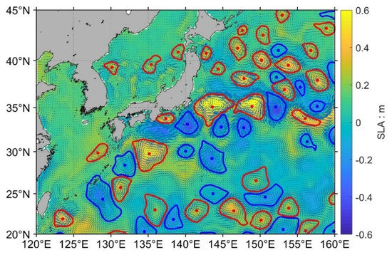
Figure 2.
The distribution of Sea Level Anomaly (SLA) and the detecting results of mesoscale eddies of the western Pacific Ocean in August 2017.
Regarding the activities on FF-SAR algorithms, the validation of the FF-SAR processors is carried out by means of analysis over point targets. Figure 3a shows the impulse response image over a simulated point target for Sentinel-6 using a local Sentinel-6 simulator, while Figure 3b shows the impulse response image retrieved from a real Sentinel-3A pass over the CDN1 transponder in Crete [50]. The across-track (AC) and along-track (AL) resolutions are estimated as the widths of the main lobes on the Impulse Response Function (IRF) 2D-image cuts on each dimension when the decay is −3dB with respect to the maximum is achieved [11]. Results are presented in Table 4 together with the theoretical resolutions, which are calculated as described in [10]. Reasonable agreement between theoretical and measured quantities is observed, which is considered a validation of the FF-SAR processor implementation for both Sentinel-3 and Sentinel-6, though for Sentinel-6, only simulated data is considered in this analysis.
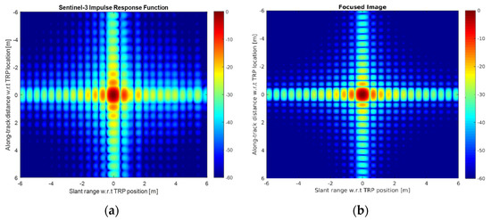
Figure 3.
(a) The 2D-focussed Impulse Response Function (IRF) of a Fully-Focussed SAR (FF-SAR) processed Sentinel-3A real pass over Crete transponder on 14 June 2019. (b) A 2D-focussed IRF of an FF-SAR processed Sentinel-6 simulated pass-over transponder. The width of the main lobe on the across-track and along-track directions provides the estimates of the across-track and along-track resolutions, respectively.
Table 4.
FF-SAR processor results over point targets.
It is worth noting that for Sentinel-3, the close-burst operation induces a pattern of ambiguities in the along-track direction. Thus, under nominal operational conditions, this effect is observed as series of replicas of the main impulse response function spaced by multiples of approximately 92 m back and forth in the along-track direction, with maximums in gain decaying with the antenna pattern attenuation. For the analysis performed in this paper, the only consequence of this feature is implicitly found in the waveforms computed over an ocean, which necessarily include contributions from these nearby replicas. Such a feature is minimized in Sentinel-6 since its radar altimeter operates in interleaved mode and the only replicas are due to the fact that after every 64-pulse burst of Ku-band pulses, there is a 1 calibration pulse followed by a 1 C-band pulse for ionospheric corrections [7], inducing minor replicas spaced by roughly 300 m in the along-track direction.
The successful implementation of the FF-SAR processors enabled the possibility to process real data from natural targets. Indeed, the results shown in this section aim at validating the performance of the FF-SAR processor for real Sentinel-3 SAR mode over an ocean. The estimation performance of the FF-SAR processing is compared with DD processing from the ESA L2 products and ESA L1B DD products with an in-house retracker. The data set used in this study consists of four tracks over the Yellow Sea recorded on 2, 9, 17 and 21 April 2020.
Figure 4 shows in blue solid line the normalized power of ESA L1B DD return waveform and FF-SAR waveform multilooked to 300 m, computed originally with an along-track resolution of 0.8 m, and a range zero-padded to 250 samples. The two echoes are returned from the closest surface location oversea. The fitted DD model is shown in red dashed line, and the text box contains the fitted parameter SWH and the Pearson correlation coefficient ρ as a measure of goodness of fit. In the case of FF-SAR waveform fitting, 180 contributing beams have been used to build the model stack. As expected, a narrowing width of the FF-SAR waveform is apparent in comparison to measured DD waveforms, in agreement with results obtained in previous studies [10]. Note that in FF-SAR processing, the incoherent averaging of single-look complex waveforms results in a smooth trailing edge of the multilook waveform, which has a direct impact on the goodness of the fit. Hence, the DD multilook model waveform is able to fairly reproduce the FF-SAR data.
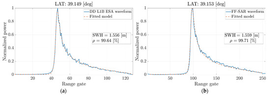
Figure 4.
Sentinel-3 open ocean normalized returned power waveforms (solid blue line) superimposed with the fitted Delay-Doppler (DD) model (red dashed line) at surfaces located around latitude 39.15 deg North on the Yellow Sea: (a) DD multilook waveform; (b) FF-SAR waveform multilooked to 300 m. The text box contains estimated Significant Wave Height (SWH) in [m] and Pearson correlation coefficient (%) as a measure of goodness of fit.
To evaluate the performance of the FF-SAR processing in the open sea, the precision of the retrieved SSH and SWH from FF-SAR and DD waveforms is analysed. For that, the averaged standard deviations of the retrieved parameters from 20 successive power waveforms, known as 20-Hz standard deviations, are computed after detrending. Similarly, the means of the retrieved SWH are calculated and subsequently sorted and arranged into bins 0.4 m wide. Finally, the means of the standard deviations of the data corresponding to each bin are calculated for SWH and SSH, denoted by <> and <>, respectively. The results obtained from the four tracks are shown in Figure 5, highlighted with different line styles. Blue triangles, orange circles, and yellow downward-pointing triangles correspond to the parameters retrieved from ESA L2, L1B DD, and FF-SAR products, respectively. Note that averaged SWH are below 2.5 m, indicating that the analysis is performed over a scenario characterised by low-average sea states. Since the precision is strongly degraded in very low sea states [51], sea states below 0.5 m have been excluded. Within this range of sea states, the general trend of the precision of the estimates from DD data is in agreement with previous results [9]. In the case of SWH from FF-SAR waveforms, shown in Figure 5a, a notable improvement with respect to DD processing is observed. This reduction approximates the factor √2 described in [10]. In addition to that, note that the precision appears to be less sensitive to sea state, which makes the FF-SAR processing highly suitable for sea state estimation. In the case of SSH, the results shown in Figure 5b indicate an overall reduced improvement of FF-SAR estimates with respect to DD, although a sea state dependency is apparent.

Figure 5.
The precision of the selected retrieved geophysical parameters from different tracks, measured as the mean of the 20-Hz standard deviations, as a function of averaged SWH, <SWH>: (a) The precision of the retrieved SWH, denoted by <>; (b) The precision of the retrieved Sea Surface Height (SSH), denoted by <>.
4.2.2. Conclusions
This study verified the accuracy of the SSH and SWH data of the new satellite data (such as Sentinel-3 and Haiyang-2 series altimeters and CFOSAT SWIM), and it is shown that the data of these satellites have high accuracy and good stability. Using multi-source satellite altimeter data, including Sentinel-3, Haiyang-2, and other altimeters, SLA is mapping, and the geostrophic current in 2018 was calculated to extract and analyse the main axis of the Kuroshio. The monthly variation characteristics of the main axis of the Kuroshio were obtained. In addition, spatial distribution and temporal variation characteristics of mesoscale eddies of the western Pacific Ocean and their movement characteristics are extracted and analysed. The results show the mesoscale eddies are greatly related to the Kuroshio in the western Pacific Ocean.
The successful FF-SAR processor implementation, confirmed with the analysis of Impulse Response Functions over simulated Sentinel-6 data and real Sentinel-3 data, has allowed testing its performance over an ocean with Sentinel-3 data. By retracking the ocean waveforms by means of a modified ocean analytical retracker, we observe a clear improvement in terms of noise in both SSH and SWH.
An assessment of the FF-SAR processor has been conducted by evaluating the precision of the retracked SWH and SSH estimates over an ocean. A DD model fitting to FF-SAR waveforms has been shown to provide a noticeable improvement of SWH precision for low-average sea states with respect to ESA L2 and L1B DD products. As regards the SSH estimates, the advantage of FF-SAR processing appears to be moderate. It is expected that future investigations on different FF-SAR configurations and sea states provide more insights into the potentiality of the FF-SAR processor for geophysical parameters retrieval.
4.3. P3 Results and Conclusions
4.3.1. Results
Following the success of SMOS interferometric radiometer measurements, two Chinese interferometers have been developed. Due to characteristics of the two different interferometric radiometers, where IMR is with a 2D Y-shaped array structure, and MICAP is with three 1D linear arrays and a reflector, IMR has 2D hexagonally sampled scenes with hexagonal-shaped cells, and MICAP is assembled with 1D scenes composed of rectangular cells (Figure 6).
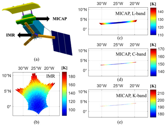
Figure 6.
An illustration of (a) the design draft of payloads Interferometric Microwave Radiometer (IMR) and Microwave Imager Combined Active and Passive (MICAP) onboard the Chinese Salinity Satellite; (b) TB (Brightness Temperature) snapshot of IMR; (c–e) TB snapshots of MICAP L-, C-, K-band radiometers respectively.
As the satellite moves, the snapshots from the continuous measurements overlap, so snapshots along the orbit are projected onto a pre-defined Earth fixed grid for the next parameter retrieval. Then, footprints of the TB measurements with information regarding polarisation, incidence angles, TB resolutions, and spatial resolutions are projected onto the matched Earth grid. Regarding the combined retrieval, the Earth grid after projection will contain measurements from both IMR and MICAP.
Monthly SSS simulations of combined retrieval have been performed. Due to the assistance of C- and K-band radiometers and the L-band scatterometer, the retrieval of SSS, SST, and WS is simultaneous. Furthermore, auxiliary information, such as SST and WS, is not required in the combined retrieval.
The monthly SSS accuracy after applying spatial-temporal averaging depends on the number of passes in different sizes of the monthly grids because more independent observations will reduce random errors caused by the TB radiometric resolution, the instrumental instability, model uncertainties, etc., in the SSS retrieval. The monthly SSS accuracy using the L-band only for both IMR and MICAP is estimated slightly worse than 0.1 psu in the 100 × 100 km grid in the global area (Figure 7). The monthly accuracy for the global area is better than 0.1 psu in the 200 × 200 km grid, and the method of combining the two payloads achieves the best monthly accuracy. Among all of these results, the monthly SSS is foreseen to achieve an accuracy of about 0.05 psu when considering all available measurements from the two payloads.
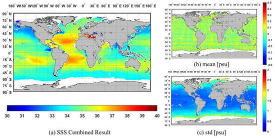
Figure 7.
Monthly Sea Surface Salinity (SSS) combined results in a 100 × 100 km grid. (a) Monthly SSS map from combined retrieval, (b) the mean value of the retrieved SSS minus the initial field, and (c) the standard deviation of the retrieved SSS compared with the initial field.
In rainy areas, the SSS retrieved from L-Band radiometers is much lower than the ones measured at a few meters’ depths or in the non-rainy surrounding regions. Since most applications are using bulk salinities, it is important to evaluate this effect. At first order, it is possible to relate the satellite SSS decrease, ∆S, observed just after a rain event to the instantaneous rain rate (RR) provided by IMERG-like products. The instantaneous effect is typically ~−1.5 pss at 10 mm h−1 [14,52]. Even when it is averaged in time and space, the signature of this effect remains larger than −0.1 psu in rainy regions such as the Intertropical Convergence Zone (Figure 8).
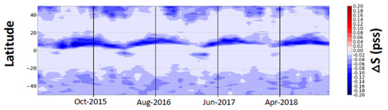
Figure 8.
The latitudinal SSS decrease due to Rain Rate (RR) events, estimated from IMERG RR and a ∆S-RR relationship similar to Figure 3 of [14].
Removing this effect from level 2 SMOS SSS retrieved from the CCI+SSS reprocessing version 3 leads to much decreased systematic differences when compared to Argo-derived salinities (Figure 9).
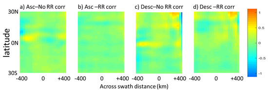
Figure 9.
Mean differences (2013–2019) of SMOS minus Argo OI SSS as a function of distance to the centre of the SMOS swath and of latitude, for ascending orbits (6AM LT) without ∆S-RR correction (a) and with ∆S-RR correction (b) and for descending orbits (6PM LT) without ∆S-RR correction (c) and with ∆S-RR correction (d).
Supply et al. in [44] also found an influence of SMAP wind speed on the ∆S-RR relationship. This could indicate a mixing effect that decreases the rain-freshening effect when the wind speed increases but also an effect of rain-induced roughness on the L-Band emissivity.
The rain-induced roughness effect was studied using the sea surface emissivity of H polarisation derived from the Aquarius L-band measurements after eliminating the emissivity of the flat sea surface using bulk in situ SSS (Figure 10). The data in rain conditions show a higher noise level than the data in non-rain conditions. When the wind speed is less than 5 m/s, the sea surface emissivity under rain conditions is much higher than the emissivity under non-rain conditions, and it does not show obvious dependency on the relative wind direction. Meanwhile, the emissivity under rain conditions approaches the non-rain emissivity under high wind speed, which indicates the wind-induced roughness effect dominates the rain-induced effect under this condition.
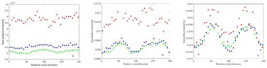
Figure 10.
H-pol sea surface emissivity under the wind speed of 5 m/s (a), 10 m/s (b), and 15 m/s (c) for RR = 0 (green dots), 0 < RR < 2 mm/h (blue dots), and RR > 2 mm/h (red dots).
We developed an empirical model that uses the L-band scatterometer data to correct the rain-induced roughness effect in the TB because the scatterometer observations are only sensitive to sea surface roughness but not sensitive to the SSS variation. Based on this model, a SSS retrieval algorithm for rain conditions is developed and validated by the Argo buoy data. The validation results show that the RMS difference of Aquarius SSS corrected for this effect with respect to in situ bulk salinities is 0.7, while it is 0.98 without correction for this effect.
A new attempt for high wind speed retrieval based on the Haiyang-2B microwave radiometer has been performed. The random forest passive (RF-passive) model was trained by using the feature parameters. The verification result of the RF-passive is shown in Figure 11. The maximum wind speed retrieved by this model is above 50 m/s. The RMSE, mean absolute error (MAE), bias, and R2 of the RF-AP model are 2.21 m/s, 1.55 m/s, 0.015 m/s, and 0.90, respectively (Figure 11).
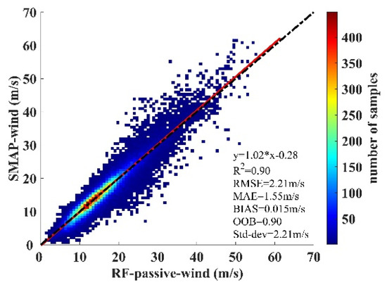
Figure 11.
Haiyang-2B wind speed versus SMAP wind speed.
Taking the wind speed 1 m/s as bin, the wind speed error of the RF-passive regression model under different wind speeds was analysed. When the wind speed is below 40 m/s, the wind speed bias is between −2 m/s and 2 m/s, and the std-dev is between 1 m/s and 3 m/s. At higher wind speeds, the absolute values of the two values are increasing, but both are within 10% of the wind speed. The results are close to the 5-year SMOS-storm database with the root mean square error on the order of 5 m/s [15].
4.3.2. Conclusions
The main conclusion on P3 are:
- (1)
- Based on the 2D and 1D characteristics of the payload IMR and MICAP, 2D IMR has a finer spatial resolution. However, as a 1D interferometric device, MICAP, with lower system complexity, achieves better TB radiometric resolution than IMR.
- (2)
- From the performance simulation, the combined retrieval with the assistance of the C- and K-band radiometers and the L-band scatterometer helps to achieve better SSS accuracy. In particular, the best SSS performance was achieved with the combination of all available measurements from the two payloads.
- (3)
- Under rainy conditions, the satellite SSS retrieved at 1 cm depth from passive L-Band measurements differs from the bulk in situ SSS by several salinity units under moderate to high rain events. When averaged spatially and temporally, the satellite SSS in rainy latitudinal bands is still underestimated by 0.1 pss or even more. Attempts have been made to correct them. Using a simple ∆S-RR relationship, we show that the main systematic differences of SMOS versus bulk in situ salinities are corrected. Alternatively, based on the combined passive and active Aquarius observations, a SSS retrieval algorithm under rain conditions is developed that decreases the RMS difference with respect to Argo bulk salinity to about 0.7 pss.
- (4)
- Based on the Haiyang-2B C-, X-, and K- bands microwave radiometer, the high wind speed retrieval algorithm during tropical cyclones is developed, and the RMS between Haiyang-2B wind and the SMAP wind is 2.21 m/s with a maximum wind speed up to 50 m/s.
5. Overall Discussion
The different activities addressed within this project have responded to the necessity of optimising the scientific yield from the data provided by the current family of Sino-European Ocean-monitoring satellites. Special efforts have been put into improving essentially the precision, accuracy, and spatial resolution of the main ocean-related physical parameters.
Regarding sea ice, increasing the robustness and accuracy of sea ice thickness retrieval is still a challenging task, in particular, regarding the availability of suitable reference data and the optimal processing of the altimetry data, which may also depend on the particular altimeter type. The major problem is that by means of altimetry, only the ice-plus-snow freeboard is directly measured; hence, the errors of the freeboard data multiply in the final thickness estimation. The retracking algorithm that we suggested [1] above has the potential to further improve thickness retrievals. With different altimetry missions in space, intercomparisons become also more and more important [32].
With the increasing number of satellite systems in space, and the development of data acquisition strategies and of advanced processing methods (e.g., machine and deep learning) based on combinations of data from different sensors (SAR, passive microwave radiometers, altimeters) or from different SAR systems (L-, C-, and X-band), the robustness and accuracy of sea ice classification will increase. With our studies [33,34], we have been contributing to questions regarding optimal classification strategies, which, e.g., also consider SAR sensor characteristics such as the change of incidence angle over range. Considering the most recent developments in methodologies for information retrieval from remote sensing data, more studies are required on optimal combinations of different sensors (which, e.g., may reveal different sensitivity to the ice characteristics or different spatial resolutions) and most suitable features derived from the different data sources (e.g., in the case of SAR, texture or polarimetric parameters).
The automated retrieval of ice drift and deformation is valuable for operational monitoring of ice conditions in the context of regional sea ice climatologies, which have also to consider the change of ice dynamics over seasons and its possible trends over years. With our analyses and improvements of drift retrieval and studies of possible errors, as discussed in Section 3.1 and Section 4.1 [35,36,37,38], we took the first steps towards the development of sea ice climatology products that also include information on ice drift and deformation.
The current Sentinel-3 and Haiyang-2A series of radar altimeters have demonstrated to be successful not only in terms of precision and accuracy when retrieving their primary products (SSH and SWH amongst others) but also in the derivation of products such as mesoscale eddies and geostrophic currents. Nevertheless, the next generation of radar altimeters and the inter-combination of their measurements will also provide a new opportunity to deepen the study of these ocean dynamic processes with improved resolutions and better performances. Indeed, upcoming radar altimeters, such as Sentinel-6 and Haiyang-2C, will represent a step forward also in terms of space-time mapping of retrieved physical variables over an ocean. Regarding future radar altimeters processing techniques, the next generation of radar altimeters is likely to include FF-SAR operational processors similar to the one presented in this paper. Indeed, targets, such as coasts and inland waters, arise as good candidates to exploit the main benefits of FF-SAR and develop new products and applications. Nonetheless, FF-SAR algorithms implemented in the time-domain as the one implemented in this project are not competitive in terms of computation time, and therefore may only be applicable to a subset of reduced targets, while other types of targets covering more extensive areas such as ocean and sea ice will require migrating from time-domain FF-SAR algorithms to frequency-domain ones. Such alternative algorithms have shown to be much more efficient [11], with computational costs that may be reduced to levels that accepted by large-scale operational processors.
For the specific case of FF-SAR performance over an ocean, a DD analytical retracker adapted to FF-SAR has performed as expected with Sentinel-3 real data and may be a realistic option for an operational processor until an FF-SAR analytical retracker is defined. The next steps here might involve (1) extending the analysis conducted here to a wider area, (2) apply it also to Sentinel-6 data whenever available and finally (3) perform a long-term time series analysis over a selection of Sentinel-3/Sentinel-6 crossing points.
Regarding the SSS topic, retrieving and validating SSS from L-Band radiometry under rainfall is very challenging. In situ measurements indicate that the salinity in the first centimetres of the ocean decreases with increasing rain rate (e.g., [53]) and that this freshening is inversely correlated to the wind speed [54]; they also indicate strong patchiness within a satellite pixel. Previous studies based on SMOS and SMAP measurements confirm dependencies of satellite salinities freshening with the rain rate and wind speed, but the sensitivities differ from the in situ observations [55]. This could reflect patchiness rain and/or wind effects, deficiencies at retrieving wind speed under rainfall, and/or additional roughness effect on the emissivity of the sea surface. Therefore, two alternative corrections are envisaged to reconcile satellite SSS and bulk salinities. The first one is only based on rain intensity, so it can be applied even if no active measurement is available at the time of the radiometer measurement. The second one is based on active L-band measurements. We show that both methods are improving the comparisons of satellites to bulk salinities. Our results reveal furthermore that the L-band active observations that are sensitive to sea surface roughness but not sensitive to SSS variation provide useful information for the empirical correction of the rain-induced effect in TB. The SSS retrieval based on the combined passive and active observations is closer to bulk SSS. Nevertheless, the physical meaning of these two empirical corrections is still a matter of debate and motivates future work. Deepened analysis of variability within satellite pixels during dedicated in situ experiments should help quantifying the influence of the heterogeneity of rain and wind in rainy pixels and their influence on the apparent signature on satellite integrated salinities. A new analysis of satellite measurements based on the concurrent active and passive measurements of future Chinese satellite missions at a better spatial resolution than Aquarius and TB simulations using a wave spectrum including rain-roughness induced effect will provide new opportunities to quantify the rain-induced roughness impact on satellite SSS.
Our results and studies from SMOS [15,16] indicate that the radiometer can obtain SSWS under high sea conditions. However, due to the problem of low spatial resolution of Haiyang-2B microwave radiometer, high spatial resolution data is needed to better invert the typhoon structure. The multi-band high radiometers onboard the Chinese SSS mission with improved ground resolution have the potential to monitor extreme wind over the sea together with SMOS.
6. Main Conclusions
The Dragon 4 project No. 32292 has promoted new satellite data applications and deliverables in several EO ocean-related fields, including improved retrievals and models for sea ice parameters, ocean waves, ocean currents, mesoscale eddies, and sea surface salinity. The improvements achieved in the different research topics addressed provide demonstrations not only of the excellent capabilities of the current European and Chinese EO satellites for ocean monitoring but also of the development and maturity of measurement and processing techniques. In addition, high perspectives are set on the potential benefits to be reported by the upcoming new generation of radar altimeters.
In terms of education, the development of the project has yield well-trained European and Chinese young scientists in the field of ocean remote sensing and has boosted their careers by giving them the opportunity to collaborate in international research networks. In addition, their integration in teams working on the exploitation of data from innovative EO satellites has allowed them to achieve the necessary know-how in cutting-edge technology and processing algorithms.
Finally, in terms of cooperation, this project has promoted the development and long-term cooperation of the European and Chinese ocean satellite remote sensing teams. The number of shared publications derived from the different developed research activities confirms the success of the project, with international collaborations expected to last for the upcoming decades.
Author Contributions
The co-authors F.G., J.B., W.D., F.G., A.G., Y.L., E.M., J.M., A.S., J.-L.V., J.W., J.Y., K.X., X.Y. and X.Z. contributed to investigation and analysis. F.G., A.G. and E.V. coordinated the edition of the manuscript. All authors have read and agreed to the published version of the manuscript.
Funding
This study was partially funded by the European Space Agency (ESA), within the frame of the ESA-MOST (Ministry of Science and Technology) Dragon 4 Cooperation (No. 4000121621/ 17/1-NB). Funding sources of the project include also Funding from the National Key Research and Development Programme of China (No. 2016YFA0600102 and No. 2018YFC1407203), and the National Nature Science Foundation of China (No. 41976173), and the Ocean Salinity Satellite Mission of China and Oceanic application with high-resolution satellites of China. The study about the influence of rain on SMOS SSS has received support from the Sea Surface Salinity Climate Change Initiative project (contract reference 4000123663/18/I-NB) funded by ESA. The European partners are in permanent positions in their organisations that support their work in this project.
Acknowledgments
Dragon 4 No. 32292 team members thank Bernat Martínez for initiating and promoting the development of this project.
Conflicts of Interest
The authors declare no conflict of interest.
Appendix A
List of relevant acronyms:
| AC | Across-track |
| AL | Along-track |
| ASCAT | Advanced SCATterometer |
| BCF | Bézier Curve Fitting |
| BDE | Boundary Definition Error |
| CFOSAT | Chinese-French Oceanic SATellite |
| CTD | Conductivity, Temperature, and Depth |
| DD | Delay-Doppler |
| EO | Earth Observation |
| FF-SAR | Fully-Focussed SAR |
| GPM | Global Precipitation Measurement |
| IMERG | Integrated Multi-satellitE Retrievals for GPM |
| IRF | Interferometric Microwave Radiometer |
| IRF | Impulse Response Function |
| L1A | Level-1 A |
| L1B | Level-1 B |
| L1C | Level-1 C |
| L2 | Level-2 |
| L3 | Level-3 |
| L3OS | Level-3 Ocean Salinity |
| MAE | Mean Absolute Error |
| MICAP | Microwave Imager Combined Active and Passive |
| MIRAS | Microwave Imaging Radiometer using Aperture Synthesis |
| NTC | Non-Time-Critical |
| OIB | Operation Ice Bridge |
| PDRE | Propagated Drift Retrieval Error |
| RA | Radar Altimetry |
| RF | Random Forest |
| RMS | Root Mean Square |
| RMSE | Root Mean Square Error |
| RR | Rain Rate |
| SAR | Synthetic Aperture Radar |
| SIRAL | SAR Interferometric Radar Altimeter |
| SLA | Sea Level Anomaly |
| SLC | Single-Look Complex |
| SMAP | Soil Moisture Active Passive |
| SMOS | Soil Moisture and Ocean Salinity |
| SRAL | Sentinel-3 Ku/C Radar Altimeter |
| SSH | Sea Surface Height |
| SSS | Sea Surface Salinity |
| SST | Sea Surface Temperature |
| SSWS | Sea Surface Wind Speeds |
| SWH | Significant Wave Height |
| SWIM | Surface Waves Investigation and Monitoring instrument |
| TB | Brightness Temperature |
| WS | Wind Speed |
Appendix B
The list of members of each sub-project is presented in Table A1.
Table A1.
List of members of the different sub-projects.
Table A1.
List of members of the different sub-projects.
| Sub-Project | Team | Member | Affiliation |
|---|---|---|---|
| P1 | Chinese | Dr. Meng Bao | First Institute of Oceanography (FIO) |
| Dr. Xi Zhang | First Institute of Oceanography (FIO) and Technology Innovation Centre for Ocean Telemetry | ||
| Dr. Bin Zou | National Satellite Ocean Application Service | ||
| Li-jian Shi | National Satellite Ocean Application Service | ||
| Chang-qing Ke | Nanjing University | ||
| Ning Wang | North China Marine Forecasting Centre | ||
| European | Prof. Wolfgang Dierking | Alfred Wegener Institute Helmholtz Centre for Polar and Marine Research and the Centre for Integrated Remote Sensing and Forecasting for Arctic Operations, The Arctic University of Norway | |
| Markku Similä | Finnish Meteorological Institute | ||
| Marko Mäkynen | Finnish Meteorological Institute | ||
| Juha Karvonen | Finnish Meteorological Institute | ||
| Rasmus Tonboe | Danish Meteorological Institute | ||
| P2 | Chinese | Dr. Yongjun Jia | National Satellite Ocean Application Service |
| Mr. Chenqing Fan | First Institute of Oceanography (FIO), Ministry of Natural Resources (MNR) | ||
| Dr. Wei Cui | First Institute of Oceanography (FIO), Ministry of Natural Resources (MNR) | ||
| Dr. Jungang Yang | First Institute of Oceanography (FIO), Ministry of Natural Resources (MNR) | ||
| European | Dr. Eduard Makhoul | isardSAT, S.L. | |
| Dr. Ferran Gibert | isardSAT, S.L. | ||
| Dr. Alba Granados | isardSAT, S.L. | ||
| P3 | Chinese | Prof. Xiaobin Yin | Ocean University of China, Qingdao |
| Dr. Yan Li | Piesat Information Technology Co., Ltd., Beijing | ||
| Dr. Kunsheng Xiang | Piesat Information Technology Co., Ltd., Beijing | ||
| Dr. Jin Wang | Qingdao University | ||
| European | Prof. Jacquelin Boutin | Sorbonne University, CNRS–IRD–MNHM and LOCEAN | |
| Dr. Alexandre Supply | LOCEAN | ||
| Dr. Jean-Luc Vergely | LOPS and ACRI-st |
Appendix C
The following papers have been written within the framework of the Dragon programs or as a collaboration between some of the Sino-European team members:
- References [1,2,3,4,40] of this publication.
- Karvonen, J.; Shi, L.; Cheng, B.; Similä, M.; Mäkynen, M.; Vihma, T. Bohai Sea Ice Parameter Estimation Based on Thermodynamic Ice Model and Earth Observation Data. Remote Sens. 2017, 9, 234.
- Yin, X.; Boutin, J.; Dinnat, E.; Song, Q.; Martin, A. Roughness and foam signature on SMOS MIRAS brightness temperatures. A semi theoretical approach. Remote Sens. 2016.
- Zeng, T.; Shi, L.; Mäkynen, M.; Cheng, B.; Zou, J.; Zhang, Z. Sea ice thickness analyses for the Bohai Sea using MODIS thermal infrared imagery. Acta Oceanol. Sin. 2016, 35, 96–104.
References
- Shen, X.; Similä, M.; Dierking, W.; Zhang, X.; Ke, C.; Liu, M.; Wang, M. A New Retracking Algorithm for Retrieving Sea Ice Freeboard from CryoSat-2 Radar Altimeter Data during Winter–Spring Transition. Remote Sens. 2019, 11, 1194. [Google Scholar] [CrossRef] [Green Version]
- Zhang, X.; Zhang, J.; Meng, J. Techniques for Sea Ice Characteristics Extraction and Sea Ice Monitoring Using Multi-Sensor Satellite Data in the Bohai Sea-Dragon 3 Programme Final Report (2012–2016). In Proceedings of the Dragon 3 Final Results and Dragon 4 Kick-Off Symposium, Wuhan, China, 4–8 July 2016. [Google Scholar]
- Garcia-Mondéjar, A.; Martínez, B.; Gao, Q.; Escorihuela, M.J.; García, P.; Yang, J.; Liao, J. Measuring the Lake Level Evolution in the Qinghai-Tibet Plateau with Radar Altimeters. In Proceedings of the Dragon 3 Final Results and Dragon 4 Kick-Off Symposium, Wuhan, China, 4–8 July 2016. [Google Scholar]
- Dierking, W.; Ji, Y.; Similä, M. The Dragon-2 Sea Ice Project: Overview and Status after Two Years. In Proceedings of the Dragon-2 Mid-Term Results Symposium 2008–2010, Guiling, China, 17–21 May 2010. [Google Scholar]
- Wingham, D.; Francis, C.; Baker, S.; Bouzinac, C.; Brockley, D.; Cullen, R.; de Chateau-Thierry, P.; Laxon, S.; Mallow, U.; Mavrocordatos, C.; et al. CryoSat: A mission to determine the fluctuations in Earth’s land and marine ice fields. Adv. Space Res. 2006, 37, 841–871. [Google Scholar] [CrossRef]
- Donlon, C.; Berruti, B.; Buongiorno, A.; Ferreira, M.-H.; Féménias, P.; Frerick, J.; Goryl, P.; Klein, U.; Laur, H.; Mavrocordatos, C.; et al. The global monitoring for environment and security (GMES) sentinel-3 mission. Remote Sens. Environ. 2012, 120, 37–57. [Google Scholar] [CrossRef]
- Donlon, C.; Cullen, R.; Giulicchi, L.; Vuilleumier, P.; Richard Francis, C.; Kuschnerus, M.; Simpson, W.; Bouridah, A.; Caleno, M.; Bertoni, R.; et al. The Copernicus Sentinel-6 mission: Enhanced continuity of satellite sea level measurements from space. Remote Sens. Environ. 2021, 258, 112395. [Google Scholar] [CrossRef]
- Raney, R.K. The delay/Doppler radar altimeter. IEEE Trans. Geosci. Remote Sens. 1998, 36, 1578–1588. [Google Scholar] [CrossRef]
- Makhoul, E.; Roca, M.; Ray, C.; Escolà, R.; Garcia-Mondéjar, A. Evaluation of the precision of different Delay-Doppler Processor (DDP) algorithms using CryoSat-2 data over open ocean. Adv. Space Res. 2018. [Google Scholar] [CrossRef]
- Egido, A.; Smith, W. Fully Focused SAR Altimetry: Theory and Applications. IEEE Trans. Geosci. Remote Sens. 2017, 1–15. [Google Scholar] [CrossRef]
- Guccione, P.; Scagliola, M.; Giudici, D. 2D Frequency Domain Fully Focused SAR Processing for High PRF Radar Altimeters. Remote Sens. 2018, 10, 1943. [Google Scholar] [CrossRef] [Green Version]
- Kleinherenbrink, M.; Naeije, M.; Slobbe, C.; Egido, A.; Smith, W. The performance of CryoSat-2 fully-focussed SAR for inland water-level estimation. Remote Sens. Environ. 2020, 237, 111589. [Google Scholar] [CrossRef]
- Reul, N.; Grodsky, S.A.; Arias, M.; Boutin, J.; Catany, R.; Chapron, B.; D’Amico, F.; Dinnat, E.; Donlon, C.; Fore, A.; et al. Sea surface salinity estimates from spaceborne L-band radiometers: An overview of the first decade of observation (2010–2019). Remote Sens. Environ. 2020, 242, 111769. [Google Scholar] [CrossRef]
- Boutin, J.; Chao, Y.; Asher, W.E.; Delcroix, T.; Drucker, R.; Drushka, K.; Kolodziejczyk, N.; Lee, T.; Reul, N.; Reverdin, G.; et al. Satellite and In Situ Salinity: Understanding Near-Surface Stratification and Subfootprint Variability. Bull. Am. Meteorol. Soc. 2016, 97, 1391–1407. [Google Scholar] [CrossRef] [Green Version]
- Reul, N.; Chapron, B.; Zabolotskikh, E.; Donlon, C.; Quilfen, Y.; Guimbard, S.; Piolle, J.F. A revised L-band radio-brightness sensitivity to extreme winds under tropical cyclones: The five year SMOS-storm database. Remote Sens. Environ. 2016, 180, 274–291. [Google Scholar] [CrossRef] [Green Version]
- Reul, N.; Tenerelli, J.; Chapron, B.; Vandemark, D.; Quilfen, Y.; Kerr, Y. SMOS satellite L-band radiometer: A new capability for ocean surface remote sensing in hurricanes. J. Geophys. Res. Oceans 2012, 117, C2. [Google Scholar] [CrossRef] [Green Version]
- ASCAT Wind Product User Manual, Ocean and Sea Ice SAF, EUMETSAT Advanced Retransmission Service, Version 1.16. 2 October 2019. Available online: https://scatterometer.knmi.nl/publications/pdf/ASCAT_Product_Manual.pdf (accessed on 1 July 2021).
- Torres, R.; Snoeij, P.M.; Davidson, M.; Bibby, D.; Lokas, S. The Sentinel-1 mission and its application capabilities. In Proceedings of the IEEE International Geoscience and Remote Sensing Symposium, Munich, Germany, 22–27 July 2012; pp. 1703–1706. [Google Scholar] [CrossRef]
- Kerr, Y.H.; Waldteufel, P.; Wigneron, J.-P.; Delwart, S.; Cabot, F.; Boutin, J.; Escorihuela, M.J.; Font, J.; Reul, N.; Gruhier, C.; et al. The SMOS Mission: New Tool for Monitoring Key Elements ofthe Global Water Cycle. Proc. IEEE 2010, 98, 666–687. [Google Scholar] [CrossRef] [Green Version]
- Li, D.; Wang, M.; Jiang, J. China’s high-resolution optical remotesensing satellites and their mapping applications. Geospat. Inf. Sci. 2021, 24, 85–94. [Google Scholar] [CrossRef]
- Sun, J.; Yu, W.; Deng, Y. The SAR Payload Design and Performance for the GF-3 Mission. Sensors 2017, 17, 2419. [Google Scholar] [CrossRef] [Green Version]
- Li, F.; Xin, L.; Guo, Y.; Gao, D.; Kong, X.; Jia, X. Super-Resolution for GaoFen-4 Remote Sensing Images. IEEE Geosci. Remote Sens. Lett. 2018, 15, 28–32. [Google Scholar] [CrossRef]
- Bao, L.; Gao, P.; Peng, H.; Jia, Y.; Shum, C.K.; Lin, M.; Guo, Q. First accuracy assessment of the HY-2A altimeter sea surface height observations: Cross-calibration results. Adv. Space Res. 2015, 55, 90–105. [Google Scholar] [CrossRef]
- Ma, C.; Zhou, W.; Yin, X.; Yu, R.; Diao, N.; Wang, S. Comparisons between HY-2B SMR and GMI brightness temperature from 6 To 37 GHz over the ocean. In Proceedings of the IGARSS 2019—IEEE International Geoscience and Remote Sensing Symposium, Yokohama, Japan, 28 July–2 August 2019; pp. 8455–8458. [Google Scholar] [CrossRef]
- Hauser, D.; Tourain, C.; Lachiver, J.M. CFOSAT: A new mission in orbit to observe simultaneously wind and waves at the ocean surface. Space Res. Today 2019, 206, 15–21. [Google Scholar]
- Huffman, G.J. GPM IMERG Final Precipitation L3 Half Hourly 0.1 Degree x 0.1 Degree V05B; Goddard Earth Sciences Data and Information Services Center (GESDISC): Greenbelt, MD, USA, 2018. [Google Scholar] [CrossRef]
- Silva, J.; Parisot, P.; Vaze, P.; Zaouche, G. Jason-3 Mission Overview. Presentation in OSTST 2016. 2016. Available online: https://meetings.aviso.altimetry.fr/fileadmin/user_upload/tx_ausyclsseminar/files/OPEN_05_OSTST_2016_Jason-3_status_gzaouche_v1-0_9h55.pdf (accessed on 1 July 2021).
- Meissner, T.; Ricciardulli, L.; Wentz, F. Capability of the SMAP Mission to Measure Ocean Surface Winds in Storms. Bull. Am. Meteorol. Soc. 2017, 98, 1660–1677. [Google Scholar] [CrossRef]
- Gaillard, F.; Reynaud, T.; Thierry, V.; Kolodziejczyk, N.; von Schuckmann, K. In Situ–Based Reanalysis of the Global Ocean Temperature and Salinity with ISAS: Variability of the Heat Content and Steric Height. J. Clim. 2016, 29, 1305–1323. Available online: https://journals.ametsoc.org/view/journals/clim/29/4/jcli-d-15-0028.1.xml (accessed on 16 July 2021). [CrossRef]
- Kolodziejczyk, N.; Prigent-Mazella, A.; Gaillard, F. ISAS-15 temperature and salinity gridded fields. SEANOE 2017. [Google Scholar] [CrossRef]
- National Data Buoy Center (NDBC) Stennis Space Center. NDBC Web Data Guide. October 2015. Available online: https://www.ndbc.noaa.gov/docs/ndbc_web_data_guide.pdf (accessed on 1 July 2021).
- Shen, X.; Ke, C.Q.; Xie, H.; Li, M.; Xia, W. A comparison of Arctic sea ice freeboard products from Sentinel-3A and CryoSat-2 data. Int. J. Remote Sens. 2020, 41, 2789–2806. [Google Scholar] [CrossRef]
- Lohse, J.; Doulgeris, A.; Dierking, W. An Optimal Decision-Tree Design Strategy and Its Application to Sea Ice Classification from SAR Imagery. Remote Sens. 2019, 11, 1574. [Google Scholar] [CrossRef] [Green Version]
- Lohse, J.; Doulgeris, A.; Dierking, W. Mapping sea-ice types from Sentinel-1 considering the surface- type dependent effect of incidence angle. Ann. Glaciol. 2020, 1–11. [Google Scholar] [CrossRef]
- Griebel, J.; Dierking, W. Impact of sea ice drift retrieval errors, discretization and grid type on calculations of sea ice deformation. Remote Sens. 2018, 10, 393. [Google Scholar] [CrossRef] [Green Version]
- Dierking, W.; Stern, H.L.; Hutchings, J.K. Estimating statistical errors in retrievals of ice velocity and deformation parameters from satellite images and buoy arrays. Cryosphere 2020, 14, 2999–3016. [Google Scholar] [CrossRef]
- Zhang, X.; Zhu, Y.; Zhang, J.; Meng, J.; Li, X.; Li, X. An Algorithm for Sea Ice Drift Retrieval Based on Trend of Ice Drift Constraints from Sentinel-1 SAR Data. J. Coast. Res. 2020, 102, 113–126. [Google Scholar] [CrossRef]
- Wang, R.; Huang, D.; Zhang, X.; Wei, P. Combined pattern matching and feature tracking for Bohai Sea ice drift detection using Gaofen-4 imagery. Int. J. Remote Sens. 2020, 41, 7486–7508. [Google Scholar] [CrossRef]
- Liang, G.; Yang, J.; Wang, J. Accuracy Evaluation of CFOSAT SWIM L2 Products Based on NDBC Buoy and Jason-3 Altimeter Data. Remote Sens. 2021, 13, 887. [Google Scholar] [CrossRef]
- Yang, J.; Zhang, J.; Cui, W.; Muñoz, M.; Makhoul, E. Primary Analysis of Oceanic Mesoscale Eddies Observation Abilities by Sentinel-3A SRAL. J. Geod. Geoinf. Sci. 2021, 4, 56–62. [Google Scholar] [CrossRef]
- Cui, W.; Wang, W.; Zhang, J.; Yang, J. Improvement of Sea Surface Height Measurements of HY-2A Satellite Altimeter Using Jason-2. Mar. Geod. 2018, 41, 632–648. [Google Scholar] [CrossRef]
- Le Traon, P.Y.; Nadal, F.; Ducet, N. An Improved Mapping Method of Multisatellite Altimeter Data. J. Atmos. Ocean. Technol. 1998, 15, 522–534. [Google Scholar] [CrossRef]
- Ray, C.; Martin-Puig, C.; Clarizia, M.P.; Ruffini, G.; Dinardo, S.; Gommenginger, C.; Benveniste, J. SAR altimeter backscattered waveform model. IEEE Trans. Geosci. Remote Sens. 2015, 53, 911–919. [Google Scholar] [CrossRef]
- Supply, A.; Boutin, J.; Reverdin, G.; Vergely, J.-L.; Bellenger, H. Variability of Satellite Sea Surface Salinity under Rainfall. In Satellite Precipitation Measurement. Advances in Global Change Research; Levizzani, V., Kidd, C., Kirschbaum, D., Kummerow, C., Nakamura, K., Turk, F., Eds.; Springer: Cham, Switzerland, 2020; Volume 69. [Google Scholar] [CrossRef]
- Mohamed, N.; Majid, A.A.; Piah, A.R.M. Data fitting by G1 rational cubic Bézier curves using harmony search. Egypt. Inform. J. 2015, 16, 175–185. [Google Scholar] [CrossRef] [Green Version]
- Yang, J.; Zhang, J.; Jia, Y.; Fan, C.; Cui, W. Validation of Sentinel-3A/3B and Jason-3 Altimeter Wind Speeds and Significant Wave Heights Using Buoy and ASCAT Data. Remote Sens. 2020, 12, 2079. [Google Scholar] [CrossRef]
- Yang, J.; Zhang, J.; Wang, C. Sentinel-3A SRAL Global Statistical Assessment and Cross-Calibration with Jason-3. Remote Sens. 2019, 11, 1573. [Google Scholar] [CrossRef] [Green Version]
- Jia, Y.; Yang, J.; Lin, M.; Zhang, Y.; Ma, C.; Fan, C. Global Assessments of the HY-2B Measurements and Cross-Calibrations with Jason-3. Remote Sens. 2020, 12, 2470. [Google Scholar] [CrossRef]
- Mulet, S.; Rio, M.-H.; Etienne, H.; Dibarboure, G.; Picot, N. The New CNES-CLS18 Mean Dynamic Topography. OceanPredict’19. Available online: https://www.godae.org/~godae-data/OP19/posters/P9-Poster_MDT18.pdf (accessed on 1 July 2021).
- Mertikas, S.; Tripolitsiotis, A.; Donlon, C.; Mavrocordatos, C.; Femenias, P.; Borde, F.; Frantzis, X.; Kokolakis, K.; Guinle, T.; Tziavos, I.; et al. The ESA Permanent Facility for Altimetry Calibration: Monitoring Performance of Radar Altimeters for Sentinel-3A, Sentinel-3B and Jason-3 Using Transponder and Sea-Surface Calibrations with FRM Standards. Remote Sens. 2020, 12, 2642. [Google Scholar] [CrossRef]
- Smith, W.; Scharroo, R. Waveform Aliasing in Satellite Radar Altimetry. IEEE Trans. Geosci. Remote Sens. 2015, 53, 1671–1682. [Google Scholar] [CrossRef]
- Supply, A.; Boutin, J.; Vergely, J.-L.; Martin, N.; Hasson, A.; Reverdin, G.; Mallet, C.; Viltard, N. Precipitation Estimates from SMOS Sea-Surface Salinity. Q. J. R. Meteorol. Soc. 2018, 144, 103–119. [Google Scholar] [CrossRef] [Green Version]
- Reverdin, G.; Supply, A.; Drushka, K.; Thompson, E.J.; Asher, W.E.; Lourenço, A. Intense and Small Freshwater Pools from Rainfall Investigated During Spurs-2 on 9 November 2017 in the Eastern Tropical Pacific. J. Geophys. Res. Oceans 2020, 125. [Google Scholar] [CrossRef]
- Kyla, D.; William, E.A.; Andrew, T.J.; Elizabeth, J.T.; Suneil, I.; Clark, D. Capturing Fresh Layers with the Surface Salinity Profiler. Oceanography 2019, 32. [Google Scholar] [CrossRef]
- Supply, A.; Boutin, J.; Vergely, J.-L.; Kolodziejczyk, N.; Reverdin, G.; Reul, N.; Tarasenko, A. New insights into SMOS sea surface salinity retrievals in the Arctic Ocean. Remote Sens. Environ. 2020, 249, 112027. [Google Scholar] [CrossRef]
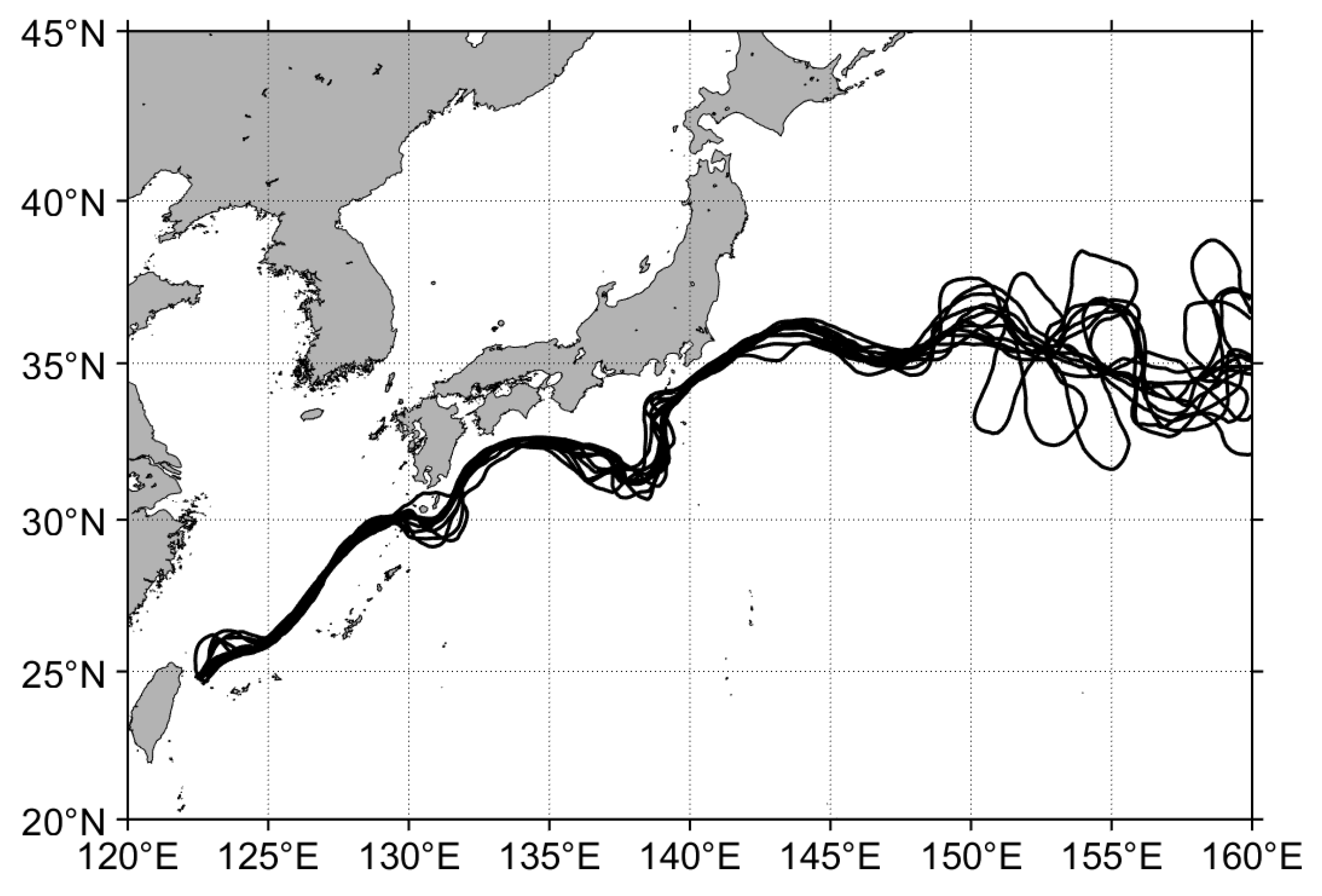
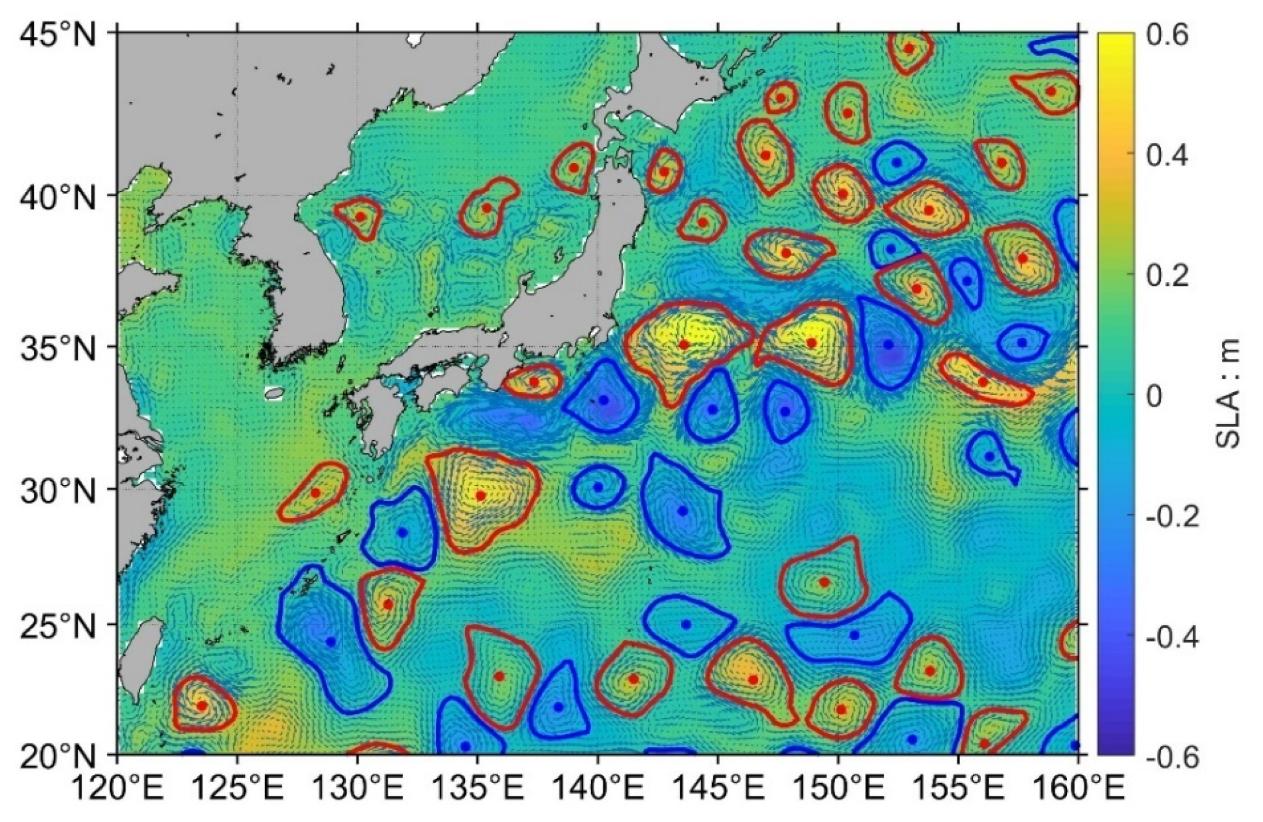
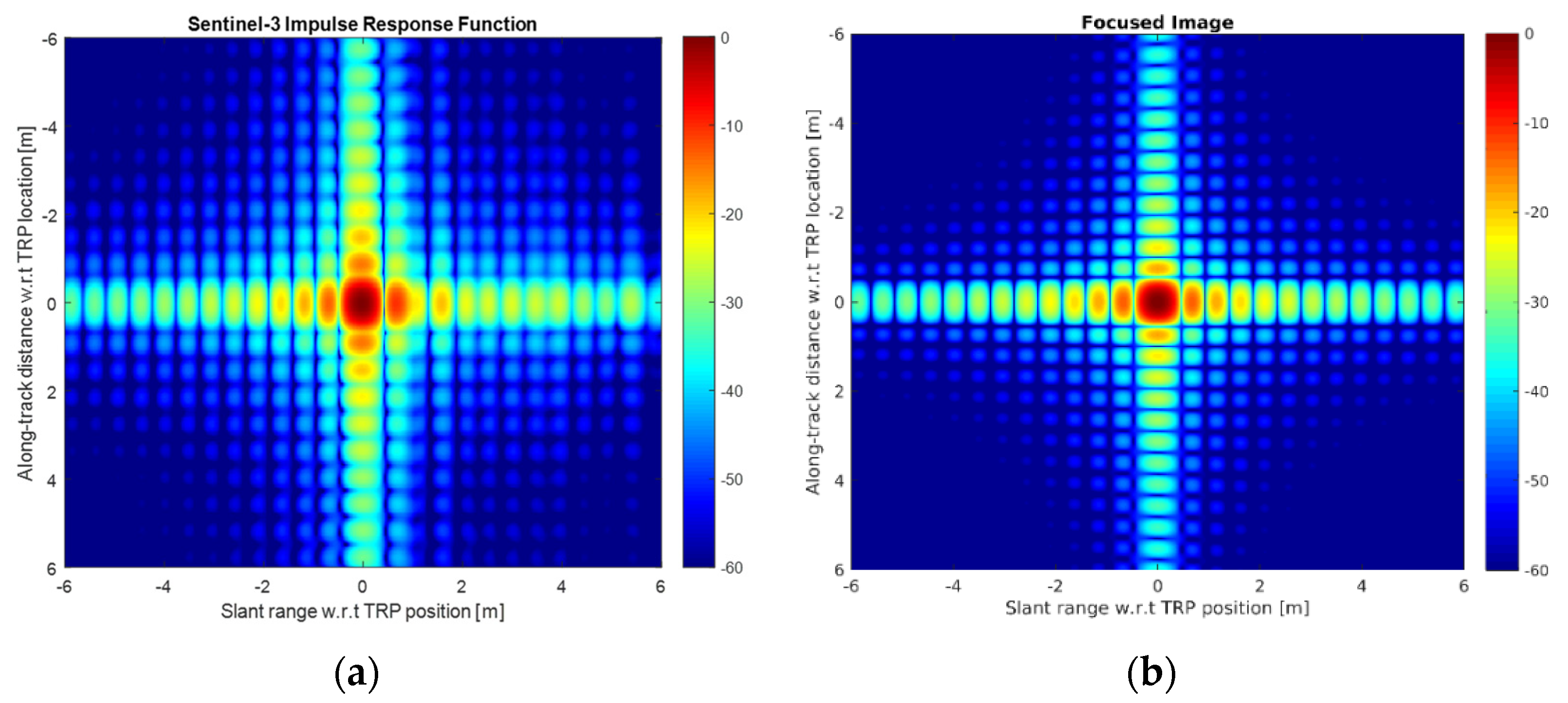
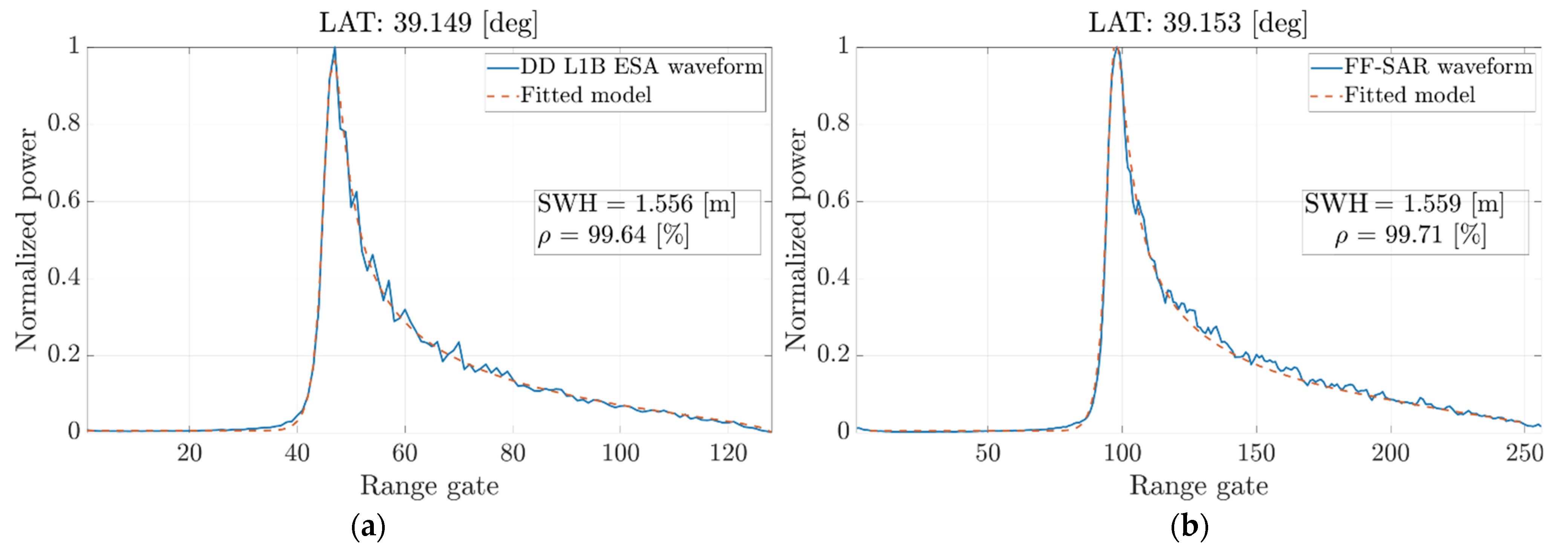
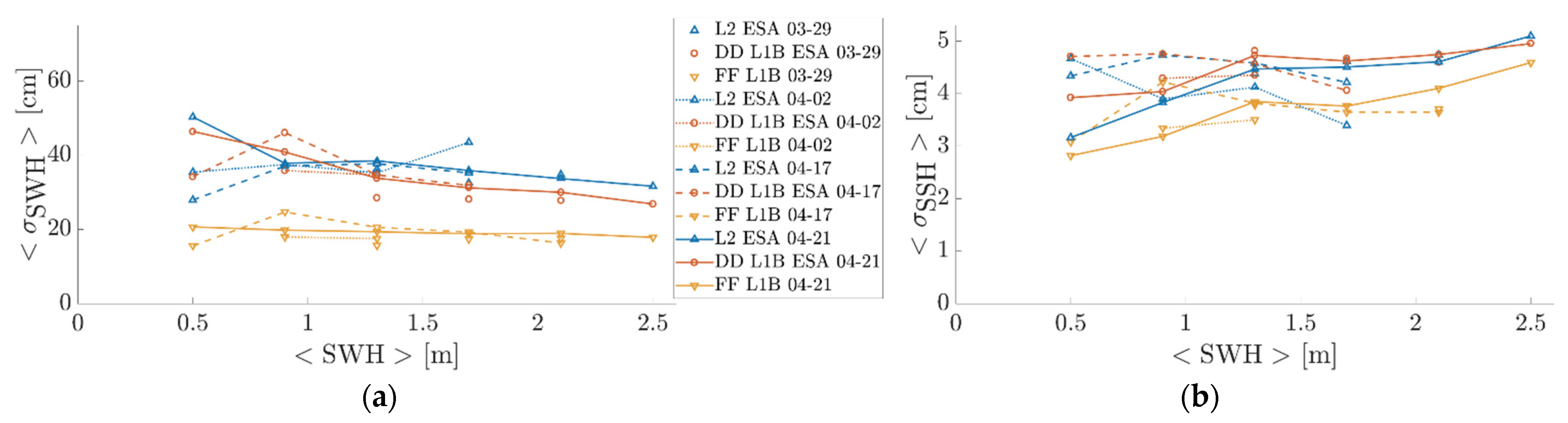
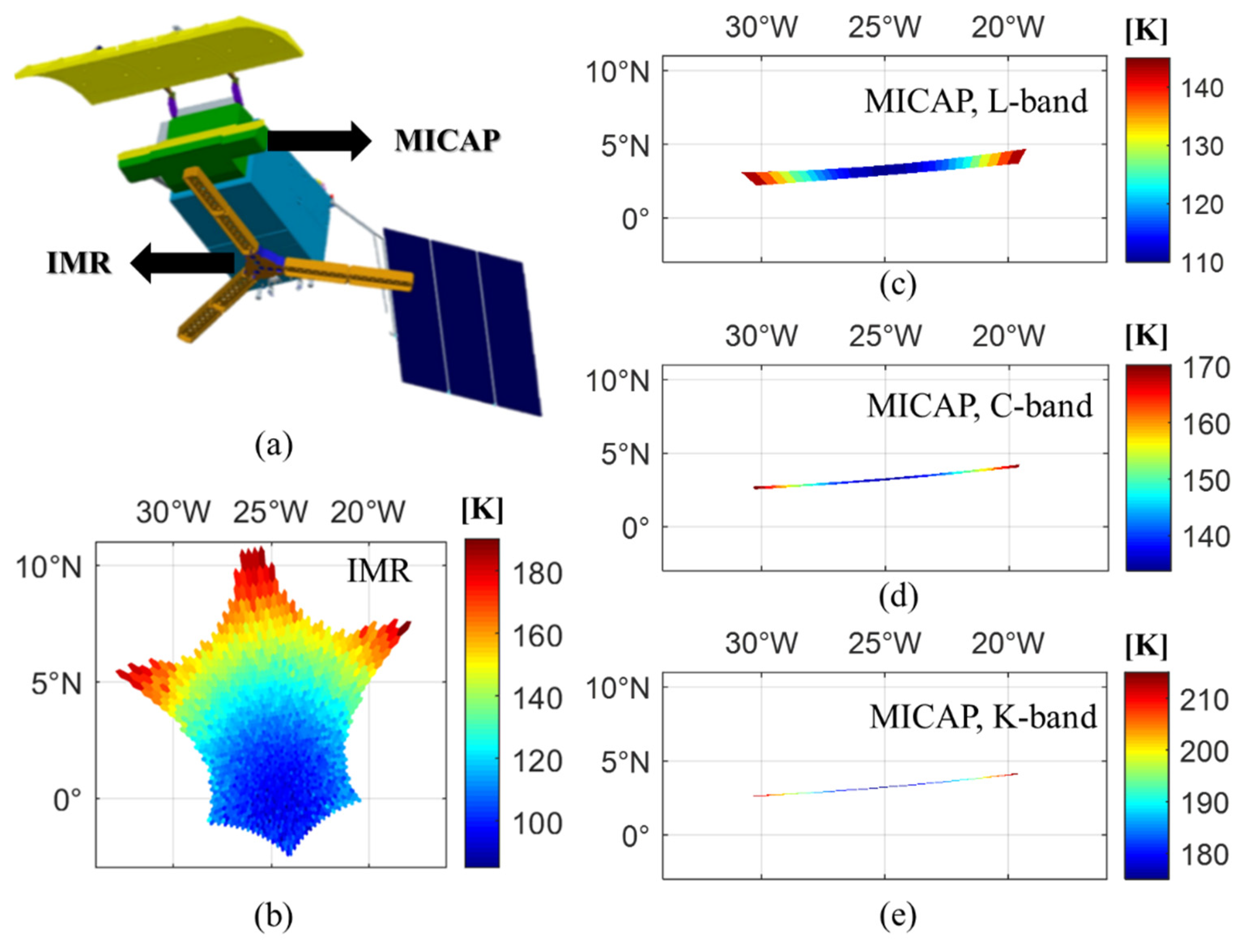

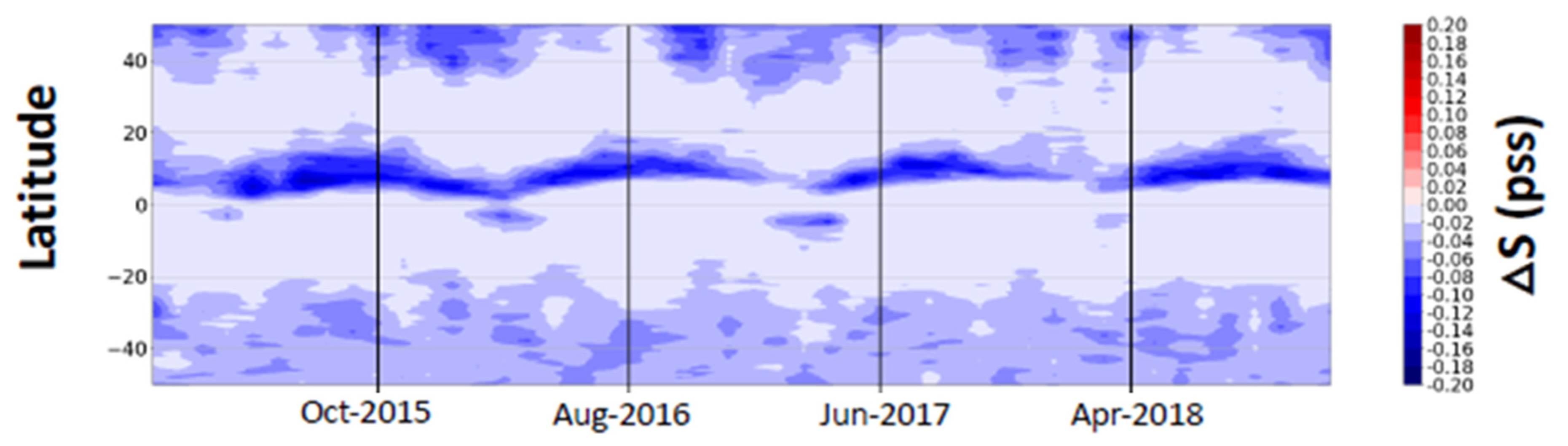
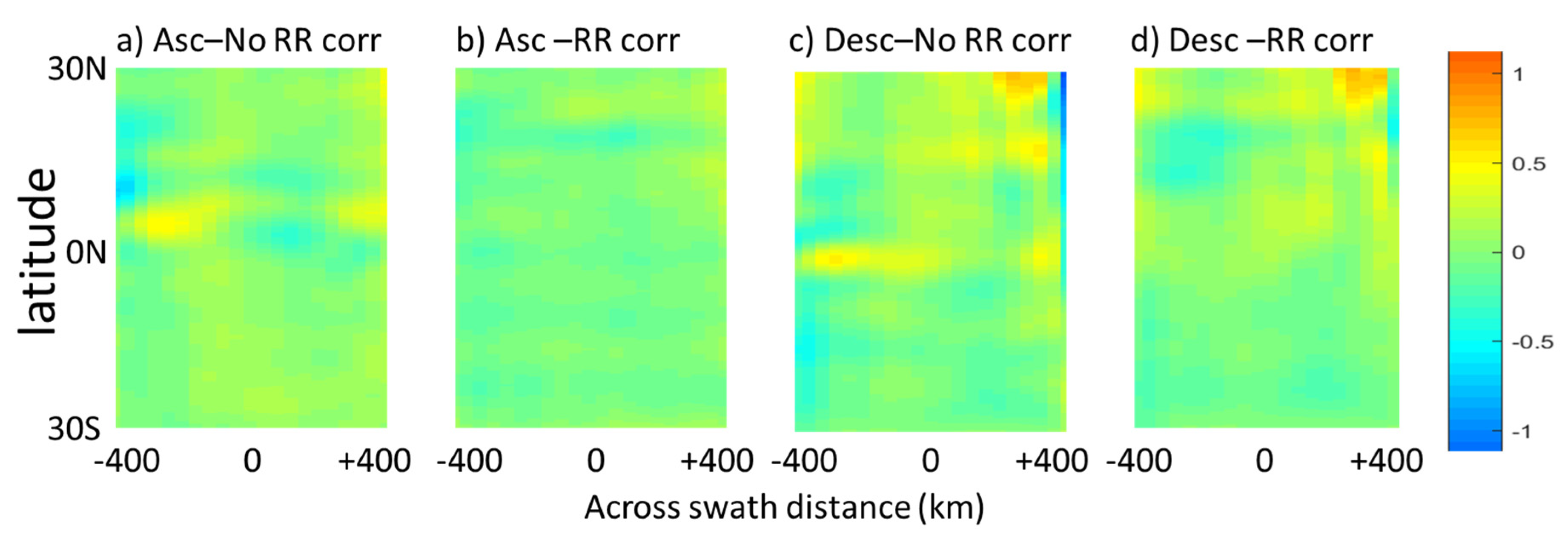
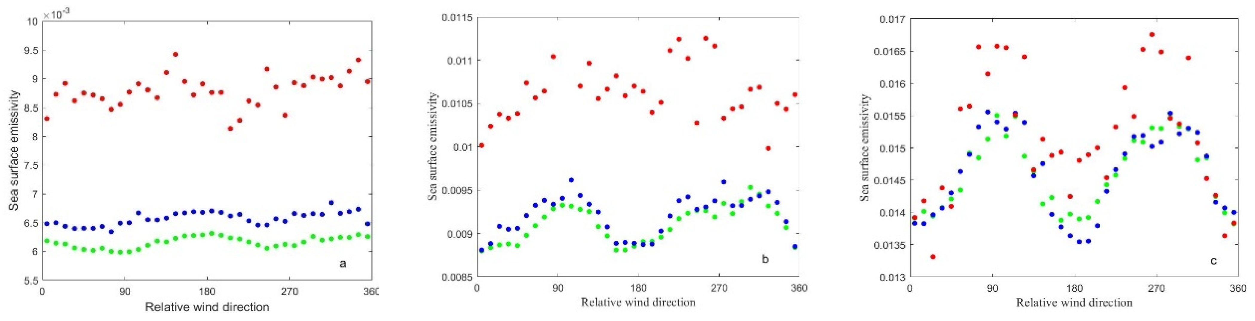

Publisher’s Note: MDPI stays neutral with regard to jurisdictional claims in published maps and institutional affiliations. |
© 2021 by the authors. Licensee MDPI, Basel, Switzerland. This article is an open access article distributed under the terms and conditions of the Creative Commons Attribution (CC BY) license (https://creativecommons.org/licenses/by/4.0/).