Article

Evaluating Machine Learning and Geostatistical Methods for Spatial Gap-Filling of Monthly ESA CCI Soil Moisture in China

College of Geoscience and Surveying Engineering, China University of Mining and Technology, Beijing 100083, China
*
Author to whom correspondence should be addressed.
Remote Sens. 2021, 13(14), 2848; https://doi.org/10.3390/rs13142848
Submission received: 10 June 2021 / Revised: 17 July 2021 / Accepted: 19 July 2021 / Published: 20 July 2021

Abstract

:
Obtaining large-scale, long-term, and spatial continuous soil moisture (SM) data is crucial for climate change, hydrology, and water resource management, etc. ESA CCI SM is such a large-scale and long-term SM (longer than 40 years until now). However, there exist data gaps, especially for the area of China, due to the limitations in remote sensing of SM such as complex topography, human-induced radio frequency interference (RFI), and vegetation disturbances, etc. The data gaps make the CCI SM data cannot achieve spatial continuity, which entails the study of gap-filling methods. In order to develop suitable methods to fill the gaps of CCI SM in the whole area of China, we compared typical Machine Learning (ML) methods, including Random Forest method (RF), Feedforward Neural Network method (FNN), and Generalized Linear Model (GLM) with a geostatistical method, i.e., Ordinary Kriging (OK) in this study. More than 30 years of passive–active combined CCI SM from 1982 to 2018 and other biophysical variables such as Normalized Difference Vegetation Index (NDVI), precipitation, air temperature, Digital Elevation Model (DEM), soil type, and in situ SM from International Soil Moisture Network (ISMN) were utilized in this study. Results indicated that: (1) the data gap of CCI SM is frequent in China, which is found not only in cold seasons and areas but also in warm seasons and areas. The ratio of gap pixel numbers to the whole pixel numbers can be greater than 80%, and its average is around 40%. (2) ML methods can fill the gaps of CCI SM all up. Among the ML methods, RF had the best performance in fitting the relationship between CCI SM and biophysical variables. (3) Over simulated gap areas, RF had a comparable performance with OK, and they outperformed the FNN and GLM methods greatly. (4) Over in situ SM networks, RF achieved better performance than the OK method. (5) We also explored various strategies for gap-filling CCI SM. Results demonstrated that the strategy of constructing a monthly model with one RF for simulating monthly average SM and another RF for simulating monthly SM disturbance achieved the best performance. Such strategy combining with the ML method such as the RF is suggested in this study for filling the gaps of CCI SM in China.

Graphical Abstract

1. Introduction

Soil moisture (SM) is a measurement of water amount in an unsaturated soil zone. It is usually expressed as the ratio of water volume to the soil volume (volumetric SM) with a unit of cm3/cm3. Soil water is the chief water resource for trees and crops growth and productivity. It also plays a significant role in land surface water and energy cycle through partitioning available energy into sensible and latent heat fluxes as well as partitioning precipitation into penetration and runoff. Therefore, acquisition of spatial continuous, i.e., gap-free SM across large areas, is crucial for many fields such as weather forecasting [1], hydrological modeling [2], agricultural productivity [3], flood forecast [4], landslide prediction [5], and drought monitoring [6,7,8].
The gap-free SM may be obtained by interpolating with ground measurements, simulating with land surface models, and retrieving from remote sensing measurements [9]. The ground stations of measuring SM are often spatially very sparse, especially at the country and continental scale. In contrast, SM usually exhibits a high spatial heterogeneity due to the effects of soil texture, structure, topographic features, land cover patterns, and meteorological forcing conditions at various scales [10]. Thus, the interpolated SM is limited to capture the complete spatial distribution of SM [11]. The simulated SM by land surface models is dependent on the number, quality, and spatial availability of forcing data, such as precipitation and solar radiation, and the model physics. Moreover, there are discrepancies between different models [9]. At present, remote sensing is becoming an effective and important tool to obtain spatially distributed SM independently to land surface models [12].
The efforts of retrieving SM from remote sensing have involved almost the whole spectrum range from visible, thermal infrared, to microwave bands [13]. Among them, the methods with optical and thermal infrared bands suffer from the common drawbacks of unavailability under cloudy weather conditions, being empirical models in most cases, and shallow penetration in soil [11,12,13,14,15,16]. Resultantly, the methods based on microwave bands are recognized as the most promising techniques. The microwave SM data resources have been reviewed in [12]. Currently, the operating space-borne sensors for microwave SM include the Advanced Microwave Scanning Radiometer at X/C-band (AMSR-E and AMSR-2), the Advanced Scatterometer (ASCAT) at C-band, WindSat Spaceborne Polarimetric Microwave Radiometer at X/C-band (WindSat), Soil Moisture and Ocean Salinity at L-band (SMOS), Soil Moisture Active Passive at L-band (SMAP), Advanced Land Observing Satellite-2 at L-band (ALOS-2), and Sentinel-1 at C-band. Among them, the AMSR-E, AMSR-2, WindSat, and SMOS are passive microwave sensors, while the ASCAT, ALOS-2, and Sentinel-1 are active microwave sensors. The SMAP integrates the passive and active microwave sensors by carrying two payloads: a real aperture radiometer and a Synthetic Aperture Radar (SAR). Based on these microwave sensors, varied single-sensor SM products were produced.
However, single sensor SM products are clearly too short to support climate monitoring and forecasting. There are some specifications of satellite SM for climate monitoring listed in [17] based on the requirements of the Global Climate Observing System (GCOS), Committee of Earth Observation Satellites (CEOS), and Climate Change Initiative (CCI) Climate Modelling User Group (CMUG). Within the specifications, the record length should be greater than 30 years. To fulfill this requirement, ESA developed a long-term SM product named ESA CCI SM through merging multiple active and passive microwave sensors. This long-term merged SM product has been evaluated in varied researches, and it has been demonstrated that the merged products have a similar or better performance than single-sensor products [18,19]. From the first version of ESA CCI SM released in 2012, this product has been updated several times at regular intervals. More and more microwave sensors would be introduced in producing merged CCI SM. Combining more single-sensor SM products could increase the likelihood of having at least one observation for a given pixel, thus reducing the number of data gaps. Nevertheless, the data gaps associated with different satellite revisit times [2028] and the physical limitations in retrieving SM by microwave observations, such as complex topography, human-induced radio frequency interference (RFI), vegetation, or snow and ice, cannot be mitigated by increasing the number of sensors or improving the blending techniques [17]. The data gaps make the SM dataset discontinuous in space and time, which limits its application in supporting climate research [1], driving the hydrological model [2], and monitoring drought [6,7,8], etc. This entails the development of gap-filling technology for ESA CCI SM [20].
Currently, the methods developed for gap-filling ESA CCI SM can be classified as the spatial interpolation method (e.g., Ordinary Kriging, OK) [21], linear regression method (e.g., Generalized Linear Model, GLM) [22], the method combining spatial interpolation and linear regression (e.g., Regression Kriging, RK) [23,24], and machine learning methods (e.g., Support Vector Machine, SVM). Llamas, Guevara, Rorabaugh, Taufer, and Vargas [21] compared the OK, RK, and GLM methods over the Midwestern United States. Their results demonstrated that geostatistical approaches (OK and RK) are better than GLM and highlight the potential of using geostatistical techniques for gap-filling. Except for the ESA CCI SM, some other gap-filling methods were applied to different global products derived from satellite images. Wang, Garcia, etc. introduced a three-dimensional method to fill the gaps in global soil moisture product based on discrete cosine transforms while using the information from both space and time [25]; Kandasamy used eight methods (i.e., iterative caterpillar singular spectrum analysis, ICSSA; empirical mode decomposition, EMD; low pass filtering, LPF; Whittaker smoother, Whit; adaptive Savitzky–Golay filter, SGF; temporal smoothing and gap filling, TSGF; asymmetric Gaussian function, AGF and the simple climatological LAI yearly profile, Clim) to fill the gaps in MODIS LAI products [26]; Hung, Seokhyeon, etc. also used the smoothing method to LST at the continental scale. [27]
In this study, we focus on filling data gaps of ESA CCI SM over the whole area of China. This study area possesses more complex terrain, various land cover, and climate features. For such an area, the relative performance of different methods may be transformed. In order to develop a suitable gap-filling method of CCI SM for the whole area of China, we compared typical Machine Learning (ML) methods, including Random Forest method (RF), Feedforward Neural Network method (FNN), and Generalized Linear Model (GLM) with the geostatistical method, i.e., OK method. The OK method was selected because it has been employed and suggested in a previous study for the gap-filling of CCI SM [21]. More than 30 years of ESA CCI SM from 1982 to 2018 and other supplementary materials in the whole area of China such as Normalized Difference Vegetation Index (NDVI), precipitation, air temperature, Digital Elevation Model (DEM), and soil type were utilized in this study. The following sections introduced the details of the study methods and materials.

2. Materials and Methods

2.1. Study Area

The mainland of China was selected as the study area with a longitude from 72°E to 135°E and latitude ranges from 18°N to 54°N. The study area has complex internal terrain and multiple climate types, which lead to the heterogeneous soil types. Figure 1 presents the spatial distribution of our study area and the soil types data. There are five black boxes in Figure 1, which are randomly selected areas for simulating data gaps in order to evaluate the gap-filling methods. Additionally, Figure 1 also presents three in situ soil moisture monitoring networks collected from the International Soil Moisture Network (ISMN) database, i.e., CHINA, CTP_SMTMN, and MAQU.

2.2. Gap-Filling Methods

Four methods were utilized in this study for conducting spatial gap-filling of CCI SM, including FNN, RF, GLM, and OK, where the former three methods are typical ML methods, and the last one is a typical geostatistical approach.
The FNN belongs to a category of Artificial Neural Network (ANN), where information only travels forward through the input nodes, hidden layers, and output nodes. In this study, the FNN was implemented using ENVI/IDL, where FNN consists of three layers. There are 10 nodes in input layer, 26 nodes in hidden layer, and 1 node for the output layer. The learning parameter was set as 0.1, and the training iteration was taken as 300. The activation function was set as sigmoid.
The RF is an ensemble learning method that operates by constructing a multitude of decision trees at training time and outputting the mean prediction of the individual trees. In this study, an open-source and robust library for ML in Python was used for implementing RF method, i.e., scikit-learning. The number of trees in the forest was set as 100. The size of the random subsets of features to consider when splitting a node is None, implying that always considering all features instead of a random subset. Additionally, we set max_depth=None in combination with min_samples_split=5.
The GLM is a representation of multivariate regression models, which describe the linear relationship between the dependent variable and predictor variables. In this study, the same scikit-learning library of ML was used to perform the GLM method. There were 10 coefficients for predictor variables and 1 intercept for the error term in the GLM model.
The implementation of the above ML methods can be expressed used the following equation:
θ = f ( NDVI ,   P ,   T a m a x ,   T a m i n ,   T a m e a n ,   DEM ,   S ,   lat , log ,   Time )
where the independent variables are NDVI, accumulated precipitation (P), the maximum air temperature ( T a m a x ), minimum air temperature ( T a m i n ), mean air temperature ( T a m e a n ), DEM, soil type (S), longitude (log), latitude (lat), and time. In this study, the ML method was trained and applied for each month. In other words, each month has a model as shown in Equation (1), and the variable Time in Equation (1) is year. The Time is actually a timestamp. It was transformed into standardized image as other ancillary variables such as NDVI. For the training part of ML methods, the first step we completed was preparing ESA CCI SM and ancillary datasets in a month scale. Specifications about the preparation can be seen in the Section 2.4. Independent variables formed a multidimensional array, then the array was put into the ML training procedure (i.e., FNN, RF, GLM models for each month). After the training, we saved the ML model files for further predicting. Relying on the gap-free ancillary variables and the regression relationship constructed by the ML models, the value of pixels in gaps were predicted and then were filled up.
The OK method uses statistical strategy to find out and describe the spatial autocorrelation of satellite-derived soil moisture in a quantificational way. The OK method was performed on the ArcGIS platform with version 10.6. We selected a spherical semi-variogram model, which is more frequently used as a suggested option; the lag-size and the cell size of output images were set as 0.25 degrees. Besides, the search radius was set as 2 degrees which is 8 times size of the ESA CCI soil moisture cells, and the 2 degrees search radius was a moderate choice due to the different situations of gaps over the region of China. At last, the range of kriging model was automatically generated by the kriging module of ArcGIS. The predicted values of missing pixels could be viewed as a linear combination of surrounding valid pixels, which can be expressed using the following equation:
Z ( s 0 ) = i = 0 N λ i Z ( s i )
where λ i represents the weight value of pixel i , the weight sum must be equal to 1; thus, estimations fulfill the unbiasedness requirement. Z ( s i ) is the soil moisture value of pixel i . Z ( s 0 ) represents the predicted value of unsampled pixels.

2.3. Evaluation Methods

The gap-filling methods were evaluated in three aspects. (1) First, they were evaluated over the whole study area, mainly concerning their ability in fitting the original CCI SM. The evaluation indexes include unbiased root-mean-square error (ubRMSE), root-mean-square error (RMSE), correlation coefficient (R), and BIAS [28]. (2) Second, the gap-filling methods were evaluated by comparing the simulated SM with the original SM data over the simulated gap areas. Five human-made SM data gaps were created, as shown in Figure 1. We deliberately removed the original ESA CCI SM in these regions, assuming that they are gaps. Subsequently, these simulated gaps were then filled with varied gap-filling methods. Finally, the gap-filled SM was compared with the original SM over these human-made gaps. (3) Third, the gap-filling methods were evaluated using in situ SM observations. The gap-filled SM were compared to the 5 cm-depth SM observations extracted from the ISMN stations. Every available observation in ISMN sites was coupled with the values in gap-filled SM during the study period. The ubRMSE, RMSE, R, and BIAS were calculated using all matching data in each site. These evaluation indexes over all sites in a network were then analyzed using box statistics.

2.4. Materials and Preprocessing

2.4.1. ESA CCI SM

The ESA CCI soil moisture dataset in a version of 4.5 was used in this study. This SM dataset has three kinds of products, i.e., the active microwave data, the passive microwave data, and the combination of them. In this study, the last one was employed for evaluating the above-mentioned gap-filling methods. The collected SM product has a temporal resolution of one-day and a spatial resolution of 0.25° spanning from November 1978 to December 2018. For convenience, we merged the daily SM into monthly SM using averaging method.

2.4.2. Ancillary Materials

(1)
Normalized Difference Vegetation Index
Since the study time of CCI SM spans from 1978 to 2018, two datasets of NDVI were utilized. The first one is GIMMS NDVI that generated from NOAA AVHRR, which covers the time from 1982 to 2000. The GIMMS NDVI has a spatial resolution of 0.083 degrees. The second one is MODIS NDVI covering the time from 2001 to 2018. The MODIS NDVI was acquired from the product of MOD13C2 - MODIS/Terra Vegetation Indices Monthly L3 Global 0.05 Deg CMG. Both the GIMMS NDVI and MODIS NDVI products have higher spatial resolution than the ESA CCI soil moisture. Thus, we aggregated the higher-resolution NDVI products into the spatial resolution of ESA CCI SM using averaging method.
(2)
Precipitation and Temperature of China
The accumulated precipitation and the maximum air temperature, minimum air temperature, and mean air temperature were acquired from China Meteorological Data Service Center, CMDC (http://data.cma.cn/en accessed on 10 June 2021). The meteorological data were gathered by National Meteorological Information Center from 2472 ground stations all over China. The meteorological data from ground stations, including accumulated precipitation and air temperature, were interpolated into gridded data at 0.5 degrees of spatial resolution using Thin Plate Spline method of ANUSPLIN (https://fennerschool.anu.edu.au/research/products/anusplin accessed on 20 July 2021) software. In order to ensure that the meteorological data could match the CCI SM, we resampled them to 0.25 degrees by means of the cubic convolution.
(3)
GTOPO30 Global Digital Elevation Model (DEM)
GTOPO30 is a global digital elevation model from the U.S. Geological Survey’s EROS Data Center in Sioux Falls, South Dakota. The spatial resolution of elevations in GTOPO30 is 0.0083 degrees, which is higher than the ESA CCI soil moisture. We resampled it to 0.25 degrees using aggregation methods of averaging.
(4)
Harmonized World Soil Database (HWSD)
The Harmonized World Soil Database is a 30 arc-second raster database with over 15,000 different soil mapping units that combines existing regional and national updates of soil information worldwide. The part of HWSD we used was generated by the Office for the Second National Soil Survey of China and Institute of Soil Science, Chinese Academy of Sciences, Nanjing, China. Soil maps of China consist of 12 orders, 61 great groups, 235 subgroups, and 909 families. The results were harmonized and incorporated into the HWSD database. The major soil types and subtypes were combined and expressed as a certain code; the codes we used were acquired from MU_GLOBAL field, and the codes ranged from 11,000 to 11,935. We resampled the original gridded database to 0.25 degrees of spatial resolution using the aggregation of the majority.

2.4.3. International Soil Moisture Network (ISMN) Data

In situ SM observations from the ISMN were also collected in order to establish a reference. There are three monitoring networks in the area of China, named CHINA, MAQU, and CTP-SMTMN, respectively. We extracted the in situ data at 5 cm depth of 96 observation sites from the three networks. The observing time of CHINA, MAQU, and CTP-SMTMN are 1982–1993, 2008–2010, and 2010–2016, respectively. We calculated the monthly means of SM for each observation site based on available data.
To ensure that each kind of data (e.g., NDVI, precipitation, air temperature, DEM, soil type, latitude, longitude, year, month) is suitable for putting into the ML methods, we established a unified standard for data preprocessing. The region of interest was located at China 72–135°E, 18–54°N, and the spatial resolution of all the materials was transformed into 0.25 degrees. All the materials were clipped into images that have 247 columns and 143 rows. The georeference was transformed into GCS-WGS-1984. All the information of the SM and ancillary dataset was summarized in Table 1.

3. Results and Discussion

3.1. Evaluating the Gap-Filling Methods over the Whole Area of China

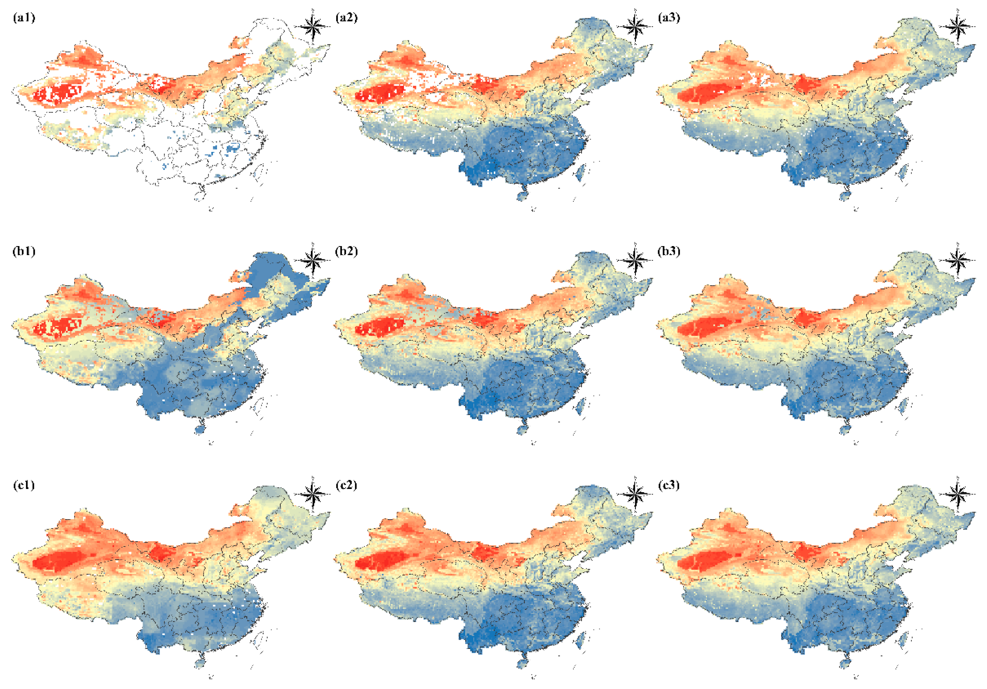
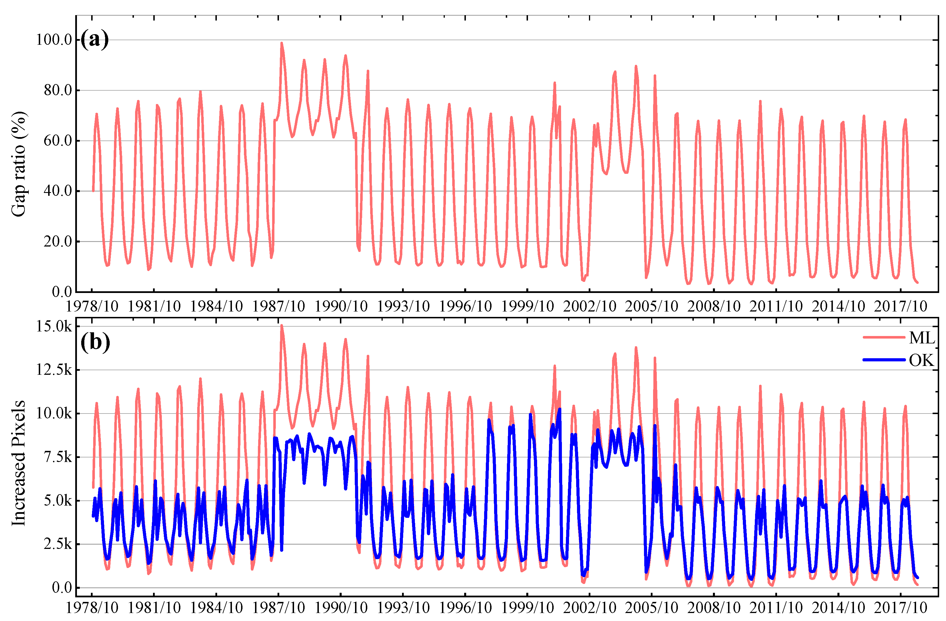
We filled the gaps of ESA CCI SM with the estimated SM generated from the above-mentioned three ML methods and the OK method. Figure 2 presents the SM data before and after gap-filling over the whole area of China in three selected months, i.e., June 1990, July 2000, and August 2010, respectively. Figure 3 presents the statistics of the gap ratio of original CCI SM, which is defined as the ratio of gap pixel numbers to all pixel numbers and the number of filled gaps by various gap-filling methods during the whole study period.
Through analyzing the original CCI SM as shown in Figure 2(a1–a3), we found that the gaps of CCI SM in China could appear in most areas. In June 1990, most areas of China did not have a valid value of CCI SM. The gap ratio showed significant seasonal variation. Normally, the gap ratio is high in cold seasons and low in warm seasons. The maximum gap ratios during the study period can be greater than 70% and sometimes greater than 80%, while the minimum gap ratios are around 10%. The mean value of the gap ratio is around 40%. These results demonstrate that the data gap of CCI SM is frequent in China, which is not only found in cold seasons and areas but also in warm seasons and areas. It is necessary to develop suitable gap-filling methods for China.
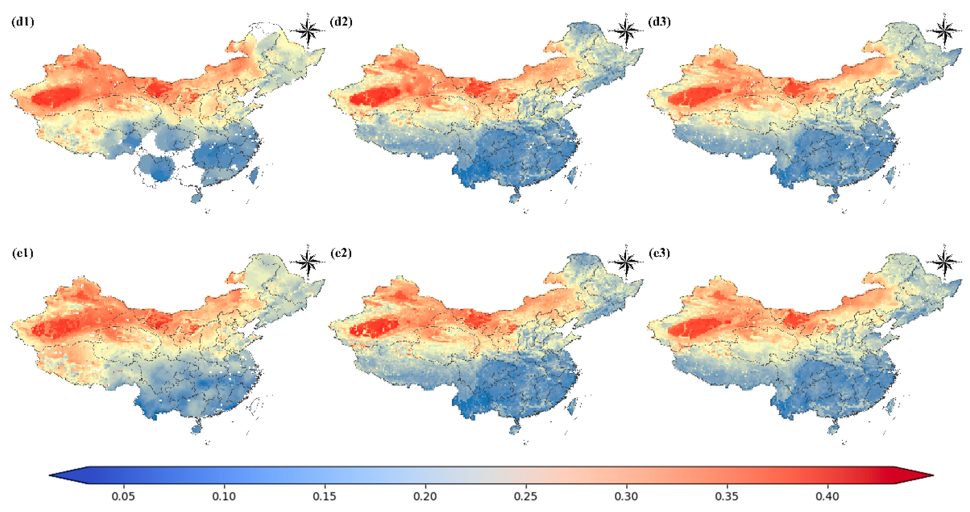
Figure 2(b1–b3) are gap-filled SM using the FNN method; Figure 2(c1–c3) are gap-filled SM using the RF method; Figure 2(d1–d3) are gap-filled SM using the OK method; and Figure 2(e1–e3) are gap-filled SM using the GLM method. The white areas in Figure 2 represent data gaps of CCI SM data. First, we found that the ML methods had a greater ability to fill up all gaps in ESA CCI SM. In contrast, the OK method would lose its gap-filling ability for areas with a wide range of gaps. This finding can be further confirmed by Figure 3b, which presents the statistics of increased pixels of gap-filled SM for different gap-filling methods. For ML methods, the increased number of gap-filled pixels can be up to 15,000 and reach an average of 5830 during the whole study period. In contrast, the numbers are 8000 and 4230 for the OK method. The three ML methods had the same number of filled pixels, and their increased pixels were much more than that by the OK method.
Figure 4 shows the comparisons between original ESA CCI SM and estimated SM with different ML methods. The boxplots were obtained by conducting statistics on the evaluation indexes of each month during the whole study period. Results showed that RF had the highest average R of 0.965, the lowest average BIAS of 1.075 × 10⁻⁴ cm3/cm3, the lowest RMSE of 0.022 cm3/cm3, and the lowest ubRMSE of 0.022 cm3/cm3. This result demonstrated that RF had the best performance in simulating the original CCI SM.

3.2. Evaluating the Gap-Filling Methods over Simulated SM Gaps

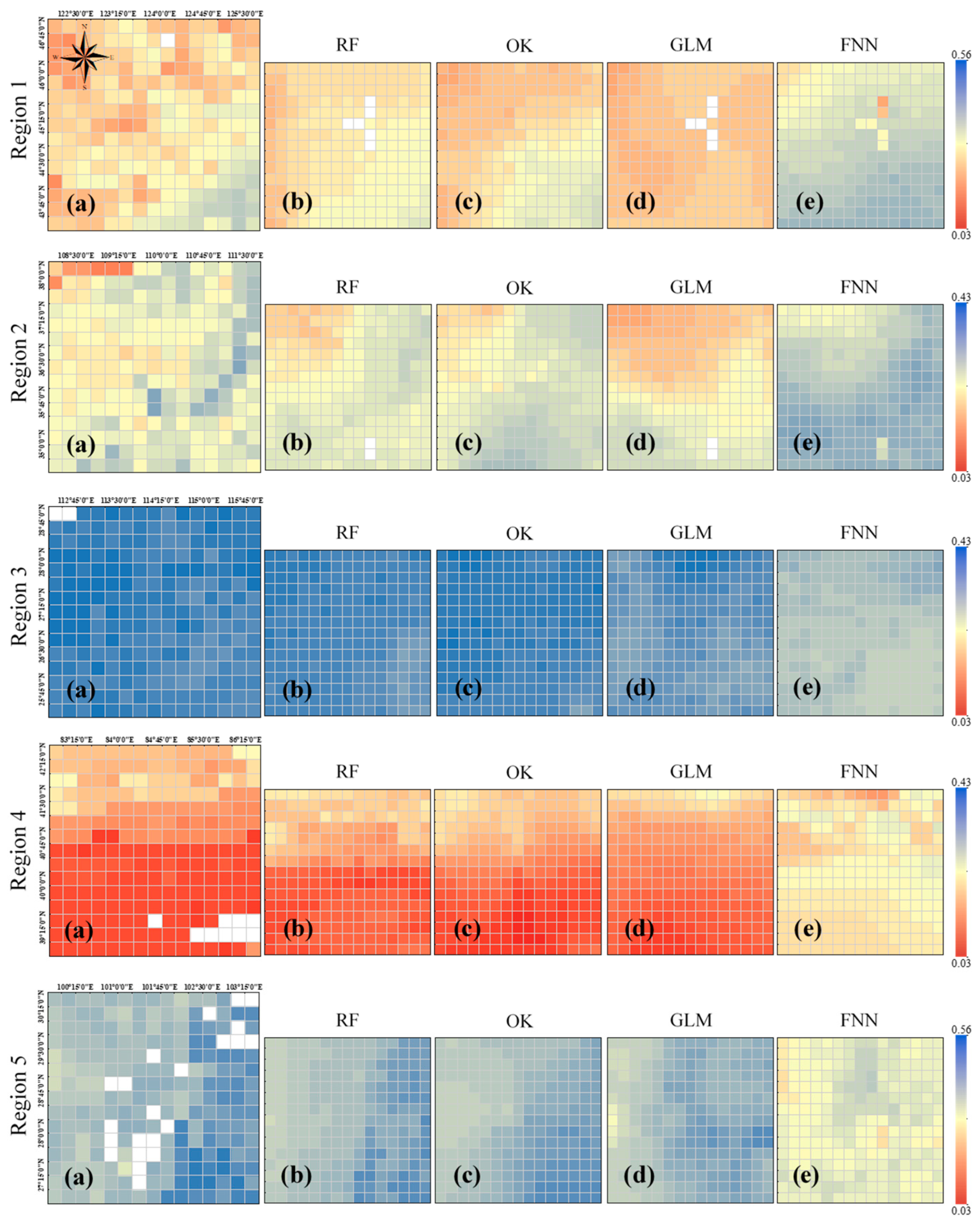
Figure 5 presents the spatial distributions of original CCI SM and simulated SM by the four gap-filling methods. According to visual recognition, we found that the distributions of original CCI SM were better depicted by the RF and OK approaches. In contrast, the data produced by FNN and GLM substantially deviated from the original ESA CCI SM.
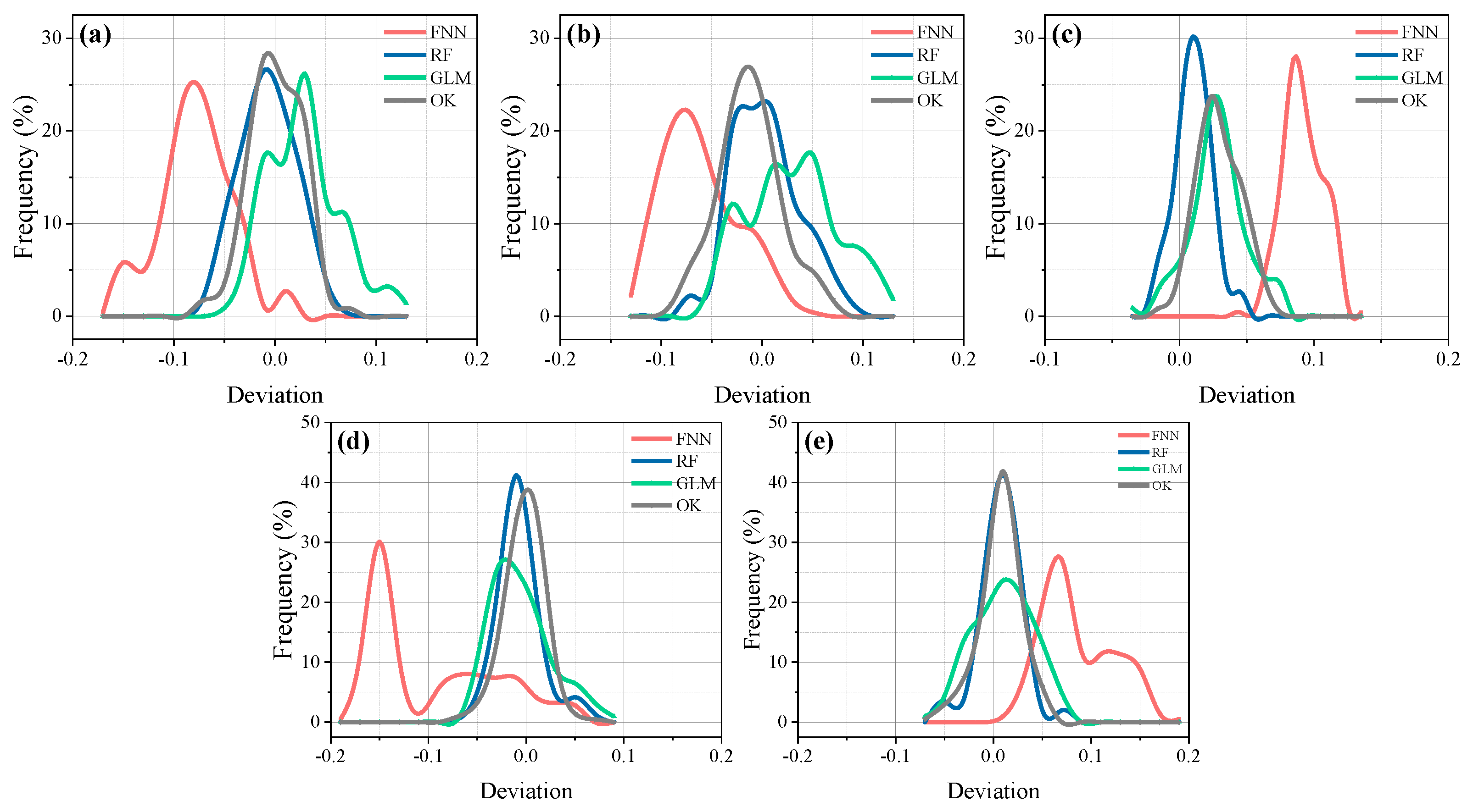
For further evaluation, we calculated the difference values between the original ESA CCI SM and the other four kinds of simulated SM in Figure 5. The statistical histograms of the differences are illustrated in Figure 6. Again, we found that most of the deviations derived by the RF and OK ranged within 0.1 cm3/cm3, which were more centralized, whereas most of the deviations derived by GLM and FNN were more scattered with an obvious bias.
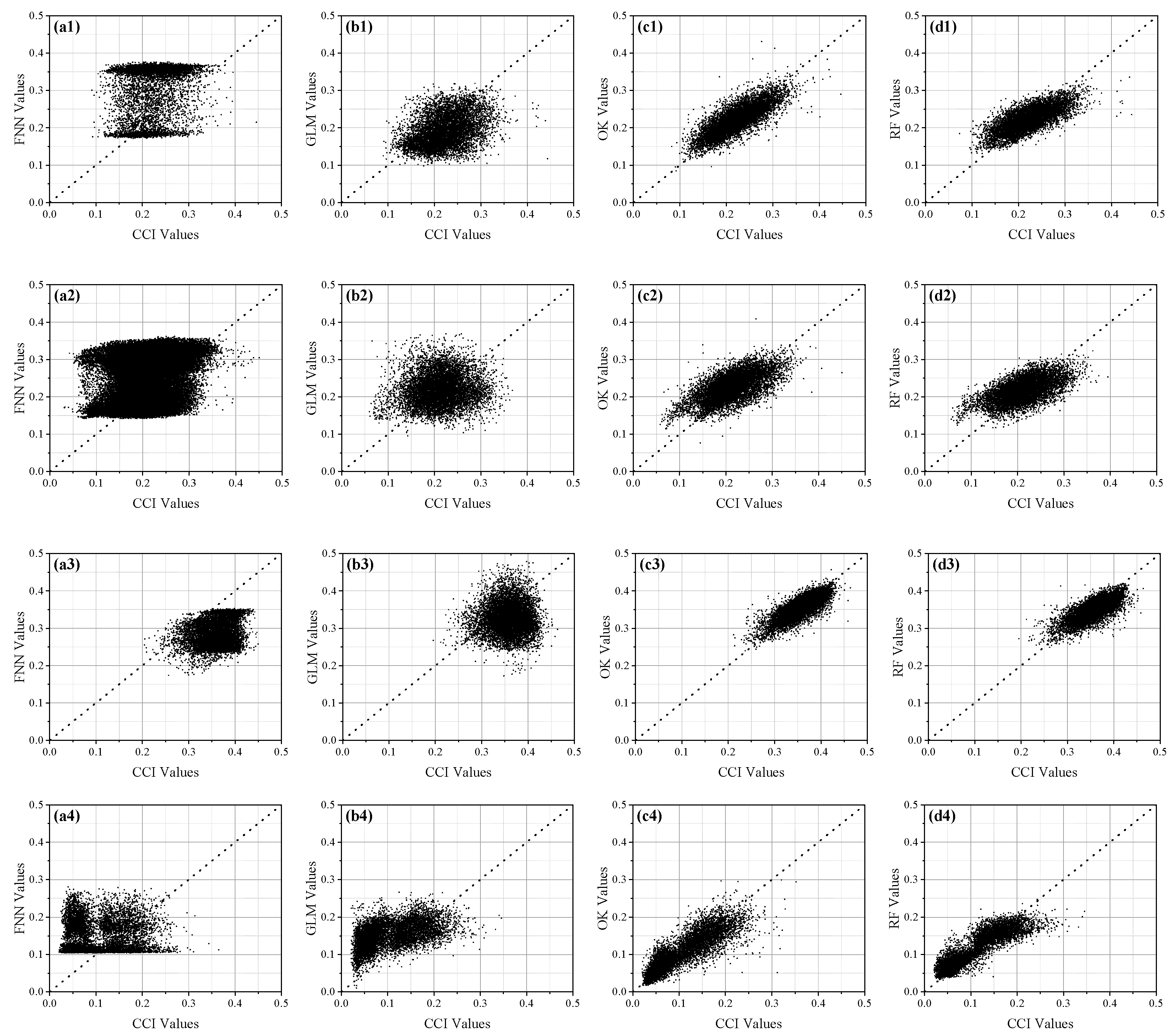
Furtherly, the comparison was extended to the whole study period. Figure 7 shows the scatter plot between original CCI SM and estimated SM by varied gap-filling methods over the whole study period. Their specific evaluation indicators are presented in Table 2, including R, R2, RMSE, ubRMSE, and BIAS. The results indicated that the average R values over the five human-made data gaps are 0.224, 0.229, 0.792, and 0.765, and the average R2 over the five gaps are 0.050, 0.052, 0.627, 0.585 for FNN, GLM, OK, and RF, respectively. The average RMSE values for them are 0.090 cm3/cm3, 0.065 cm3/cm3, 0.029 cm3/cm3, 0.030 cm3/cm3, respectively. The average ubRMSE values for them are 0.062 cm3/cm3, 0.057 cm3/cm3, 0.029 cm3/cm3, and 0.029 cm3/cm3. The average BIAS values for them are −0.014 cm3/cm3, 0.007 cm3/cm3, −0.001 cm3/cm3, and −0.001 cm3/cm3, respectively. It can thus be concluded that RF and OK methods had comparable performances in this study, and they outperformed the FNN and GLM methods greatly over the simulated data gap area.

3.3. Evaluating the Gap-Filling Methods at In Situ Stations

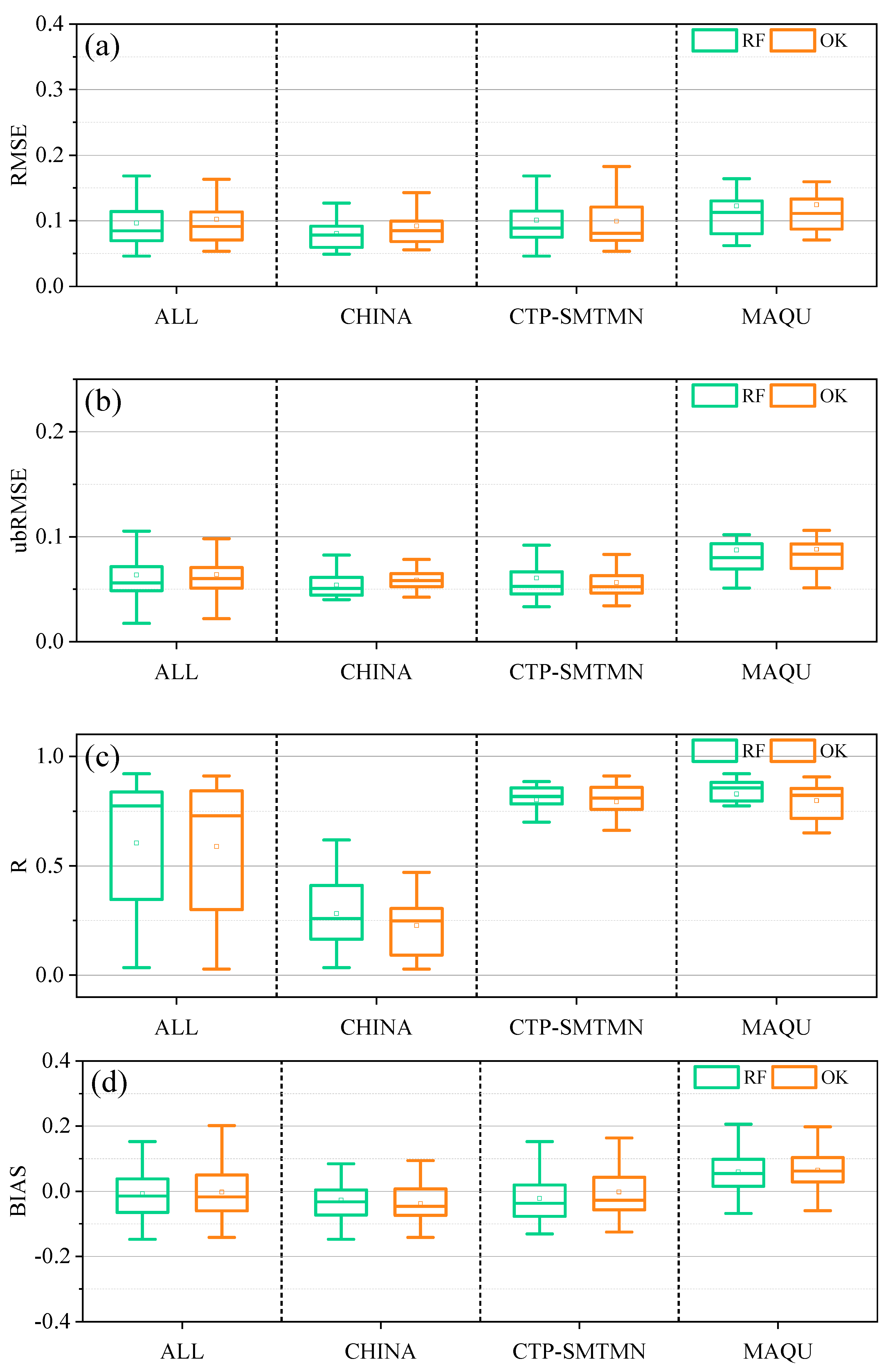
Additionally, in situ SM data from ISMN was used to evaluate the OK and ML gap-filling methods. Among the three ML methods, the above-mentioned evaluations over the whole area of China and over the simulated gaps both demonstrated that the RF method outperformed the FNN and GLM methods greatly for gap-filling. Thus, OK and RF methods were employed in this evaluation. Again, four evaluation indicators, i.e., RMSE, ubRMSE, R, and BIAS, were calculated at each observation station during the whole study period. The box plots of these indicators over each network and all networks are presented in Figure 8. There are 38 observation stations in the network of CHINA, 38 stations in CTP-SMTMN, 20 stations in MAQU, and 96 stations in ALL networks. The results indicated that the BIAS, RMSE, and ubRMSE of the RF method were slightly less than that of the OK method, while R of the RF method was slightly greater than that of the OK method. We calculated the median R and ubRMSE over all in situ stations. The median R values for RF and OK are 0.773 and 0.724, respectively. The median ubRMSE for RF and OK are 0.056 cm3/cm3 and 0.060 cm3/cm3, respectively. It can be concluded that the estimated SM by the RF method had a better consistency than that by the OK method as compared with the in situ SM.

3.4. Three Strategies for Gap-Filling Based on RF

The results in the above sections indicated that there are many gaps in CCI SM over the whole area of China, whose gap ratio can reach up to more than 80%. For the wide range of data gaps, the OK method could barely fill them all up, whereas the ML methods can. Evaluations over the whole area of China and human-made simulated SM gaps demonstrated that the RF method and OK method had comparable performances, and they both outperformed the FNN and GLM methods. As compared with in situ SM from ISMN networks, RF method performed a bit better than the OK method. Consequently, we concluded that among the OK, RF, FNN, and GLM methods we evaluated, the RF method was the most preferable for filling the CCI SM gaps in the whole area of China in this study.
With the knowledge obtained from the evaluations, it is very valuable to discuss the strategy of employing the RF method to fill the CCI SM gaps in China. Here, we constructed three strategies that can be expressed in the following equations. The first strategy can be expressed by Equation (1), which has been mentioned previously. We labeled this strategy as Strategy 1, where there is one RF model for each month.
The secondary strategy (hereafter Strategy 2) can be expressed by the following equation:
θ = f ( NDVI ,   P ,   T a m a x ,   T a m i n ,   T a m e a n ,   DEM ,   S ,   lat ,   log ,   Y ,   M )
where Y is year and M is month. The other independent variables have the same meaning as that in Equation (1). It should be noted that there is only one big RF model for all data in Strategy 2.
The third strategy (hereafter Strategy 3) includes two steps where the first step is employing RF to estimate monthly average SM, and the second step is employing RF to estimate the disturbance over the monthly average SM. The monthly average SM was modeled using the following equation:
θ ¯ = f ( lat , log , Y )
where θ ¯ represents the monthly average SM, log represents longitude, lat represents latitude, and Y represents the year of SM. Based on the monthly average SM, the monthly SM was calculated using the following equation:
θ = θ ¯ + f ( NDVI , P , T a m a x , T a m i n , T a m e a n , DEM , S , lat , log , Y )
where θ represent the monthly SM, and the second term on the right side of this equation is called monthly disturbance.
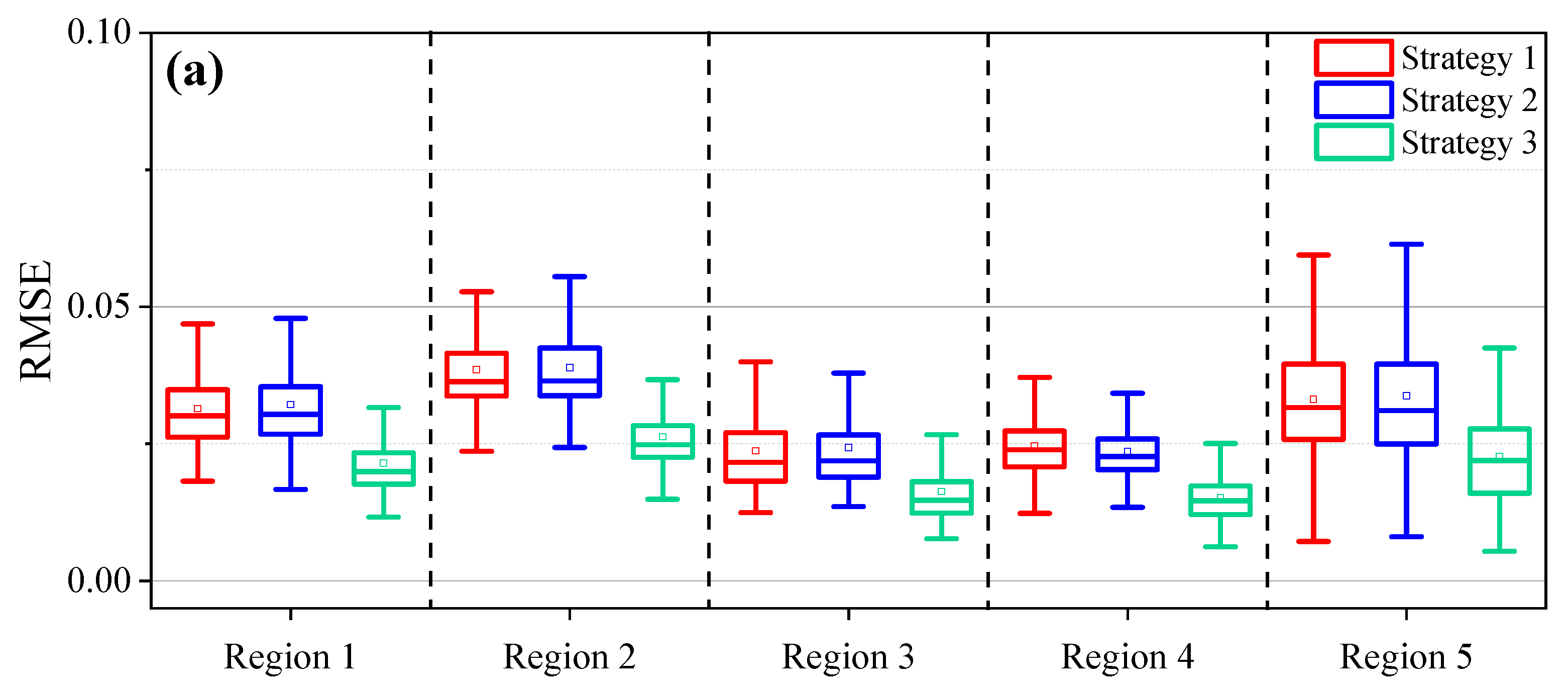
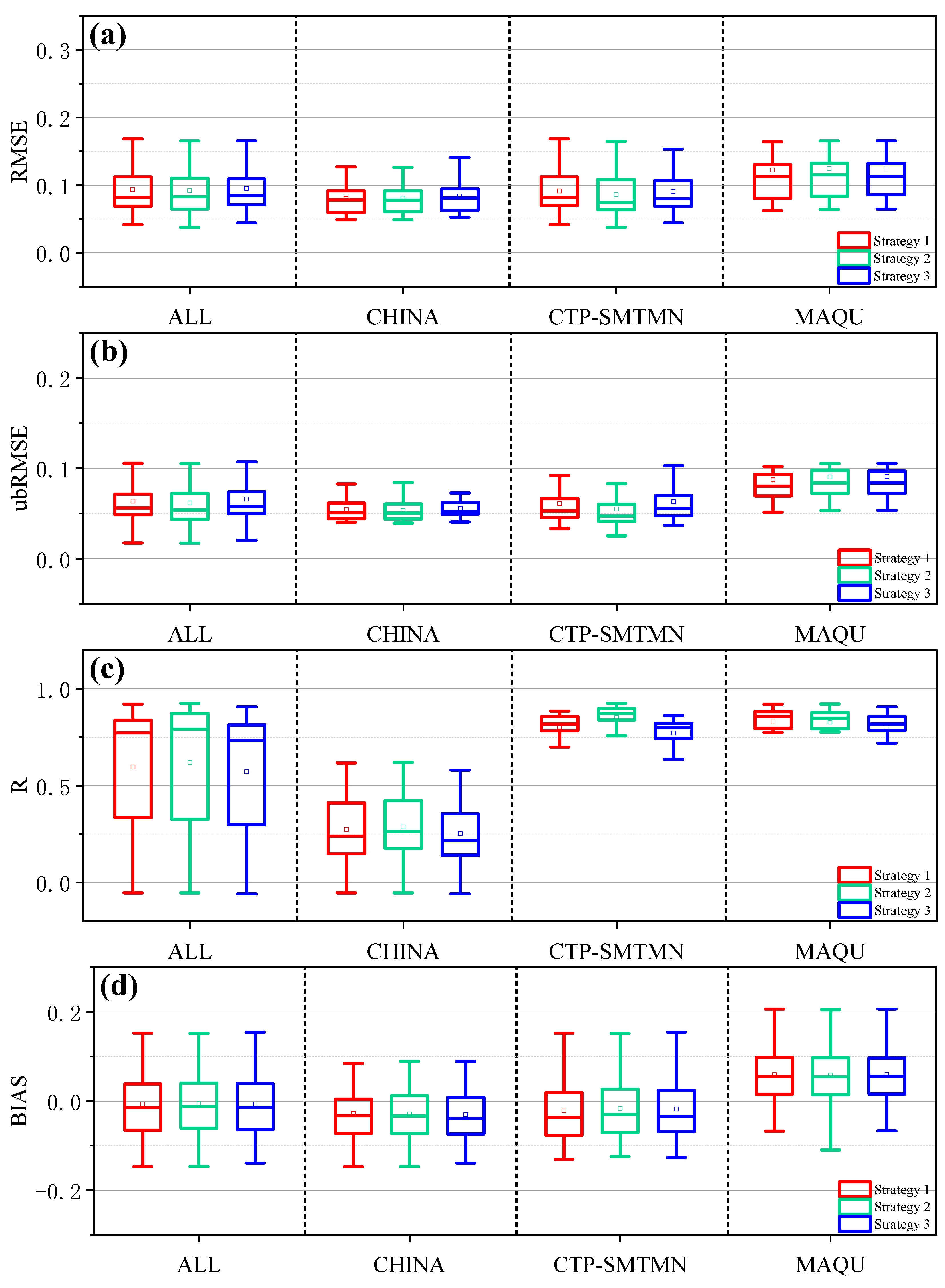
To evaluate the different strategies, we compared the estimated SM with the original SM over simulated gap areas. The four quantitative indicators RMSE, ubRMSE, R, and BIAS were employed to measure the comparisons. Results are shown in Figure 9, which clearly demonstrated that Strategy 3 had the lowest BIAS, RMSE, and ubRMSE, and the highest correlation coefficient R in each and all simulated gap areas. Figure 9 demonstrates that Strategy 3 was the best choice among the three strategies for conducting the gap-filling work.
We also compared the estimated SM by different strategies with the in situ SM. The evaluation results are shown in Figure 10. The median RMSE values at all in situ stations for Strategy 1, 2, and 3 are 0.082 cm3/cm3, 0.083 cm3/cm3, and 0.084 cm3/cm3, respectively. The median R values at all in situ stations for Strategy 1, 2, and 3 are 0.773, 0.793, and 0.732, respectively. The median ubRMSE values at all in situ stations for Strategy 1, 2, and 3 are 0.056 cm3/cm3, 0.054 cm3/cm3, 0.058 cm3/cm3, respectively. The three strategies achieved comparable performance according to the comparisons with in situ SM. However, in view of the significant relative performance in Figure 9, the gap-filling strategy using monthly average SM adding monthly SM disturbance is suggested for filling the CCI SM gaps in China.

4. Conclusions

In order to develop a suitable method to fill the gaps of ESA CCI SM in China, typical ML methods (RF, FNN, GLM) and a geostatistical method (OK) were evaluated in this study. ESA CCI SM of active + passive product (COMBINED) was selected in the evaluation. The study period spanned more than 35 years from 1982 to 2018, and various supplementary variables were utilized, such as NDVI, DEM, precipitation, temperature, soil type, and geographical location factors, etc. The evaluation was conducted over the whole area of China, over simulated gap areas, and over in situ SM stations. Results indicated that:
(1)
The data gap of CCI SM is frequent in China, which is not only found in cold seasons and areas but also in warm seasons and areas. The maximum gap ratios can be greater than 80%, and the average gap ratio is around 40%.
(2)
ML methods had a stronger gap-filling ability than the geostatistical OK method. ML methods can fill the gaps of CCI SM all up, whereas the OK method cannot. Among the evaluated ML methods, RF had the best performance in fitting the relationship between SM and biophysical variables with R of 0.965 and RMSE of 0.022 cm3/cm3.
(3)
Over five simulated gap areas, RF had comparable performance with OK, and it outperformed the FNN and GLM methods greatly. The average R values are 0.224, 0.229, 0.792, and 0.765 for FNN, GLM, OK, and RF, respectively. The average ubRMSE values for them are 0.062 cm3/cm3, 0.057 cm3/cm3, 0.029 cm3/cm3, and 0.029 cm3/cm3, respectively.
(4)
As compared with in situ SM from ISMN networks, RF achieved better performance than the OK method. The median R values at all in situ stations are 0.773 and 0.724 for RF and OK methods, respectively. The median ubRMSE at all in situ stations are 0.056 cm3/cm3 and 0.060 cm3/cm3 for RF and OK methods, respectively.
(5)
We also explored three strategies for gap-filling CCI SM based on the RF method, where Strategy 1 is creating monthly RF model for data each month, Strategy 2 is creating a big RF for all data, and Strategy 3 is also constructing monthly model but with one RF for simulating monthly average SM and another RF model for simulating monthly SM disturbance. Results indicated that Strategy 3 achieved the best performance, which is suggested for filling the CCI SM gaps in the whole area of China.
Certainly, there are some limitations in this study, where the most significant one is that only three typical ML methods and one geostatistical method were utilized. This study highlights the potential of ML methods for CCI SM gap-filling in China. The future work could introduce other ML methods such as XGBoost and lightGBM to improve the gap-filling work. Remotely sensed land surface temperature, land surface evaporative efficiency, and other land surface variables related to SM could be explored to improve furtherly the gap-filling of CCI SM. Additionally, it would be a good work in the future for studying the combination of the geostatistical method and ML method in gap-filling of CCI SM.

Author Contributions

Conceptualization, H.S.; methodology, H.S. and Q.X.; formal analysis, H.S. and Q.X.; writing—original draft preparation, H.S. and Q.X.; resources, H.S. and Q.X.; writing—review and editing, H.S. and Q.X. Both authors have read and agreed to the published version of the manuscript.

Funding

This research was funded by the National Natural Science Foundation of China, grant number 41871338; Ningxia Key Research and Development Program, grant number 2018BEG03069; Yue Qi Young Scholar Project, CUMTB2018; and Fundamental Research Funds for the Central Universities, grant number 2021YJSDC23.

Acknowledgments

The authors would like to thank the European Space Agency for providing the CCI soil moisture data. Thanks are also given to the scholar and engineer who provide the NDVI, DEM, precipitation, temperature, and soil type data.

Conflicts of Interest

The authors declare no conflict of interest.

References

  1. Collow, T.W.; Robock, A.; Wu, W. Influences of soil moisture and vegetation on convective precipitation forecasts over the United States Great Plains. J. Geophys. Res. Atmos. 2014, 119, 9338–9358. [Google Scholar] [CrossRef]
  2. Sadeghi, M.; Tuller, M.; Warrick, A.W.; Babaeian, E.; Parajuli, K.; Gohardoust, M.R.; Jones, S.B. An analytical model for estimation of land surface net water flux from near-surface soil moisture observations. J. Hydrol. 2019, 570, 26–37. [Google Scholar] [CrossRef]
  3. Ines, A.V.M.; Das, N.N.; Hansen, J.W.; Njoku, E.G. Assimilation of remotely sensed soil moisture and vegetation with a crop simulation model for maize yield prediction. Remote Sens. Environ. 2013, 138, 149–164. [Google Scholar] [CrossRef] [Green Version]
  4. Laiolo, P.; Gabellani, S.; Campo, L.; Silvestro, F.; Delogu, F.; Rudari, R.; Pulvirenti, L.; Boni, G.; Fascetti, F.; Pierdicca, N.; et al. Impact of different satellite soil moisture products on the predictions of a continuous distributed hydrological model. Int. J. Appl. Earth Obs. Geoinf. 2016, 48, 131–145. [Google Scholar] [CrossRef]
  5. Brocca, L.; Ponziani, F.; Moramarco, T.; Melone, F.; Berni, N.; Wagner, W. Improving Landslide Forecasting Using ASCAT-Derived Soil Moisture Data: A Case Study of the Torgiovannetto Landslide in Central Italy. Remote Sens. 2012, 4, 1232–1244. [Google Scholar] [CrossRef] [Green Version]
  6. AghaKouchak, A.; Farahmand, A.; Melton, F.S.; Teixeira, J.; Anderson, M.C.; Wardlow, B.D.; Hain, C.R. Remote sensing of drought: Progress, challenges and opportunities. Rev. Geophys. 2015, 53, 452–480. [Google Scholar] [CrossRef] [Green Version]
  7. Sun, H.; Chen, Y.; Sun, H. Comparisons and classification system of typical remote sensing indexes for agricultural drought. Trans. Chin. Soc. Agric. Eng. 2012, 28, 147–154. [Google Scholar] [CrossRef]
  8. Sun, H.; Zhao, X.; Chen, Y.; Gong, A.; Yang, J. A new agricultural drought monitoring index combining MODIS NDWI and day–night land surface temperatures: A case study in China. Int. J. Remote Sens. 2013, 34, 8986–9001. Available online: https://doi.org/10.1080/01431161.2013.860659 (accessed on 20 July 2021). [CrossRef]
  9. Seneviratne, S.I.; Corti, T.; Davin, E.L.; Hirschi, M.; Jaeger, E.B.; Lehner, I.; Orlowsky, B.; Teuling, A.J. Investigating soil moisture-climate interactions in a changing climate: A review. Earth-Sci. Rev. 2010, 99, 125–161. [Google Scholar] [CrossRef]
  10. Crow, W.T.; Berg, A.A.; Cosh, M.H.; Loew, A.; Mohanty, B.P.; Panciera, R.; de Rosnay, P.; Ryu, D.; Walker, J.P. Upscaling sparse ground-based soil moisture observations for the validation of coarse-resolution satellite soil moisture products. Rev. Geophys. 2012, 50, RG2002. [Google Scholar] [CrossRef] [Green Version]
  11. Peng, J.; Loew, A.; Merlin, O.; Verhoest, N.E.C. A review of spatial downscaling of satellite remotely sensed soil moisture. Rev. Geophys. 2017, 55, 341–366. [Google Scholar] [CrossRef]
  12. Babaeian, E.; Sadeghi, M.; Jones, S.B.; Montzka, C.; Vereecken, H.; Tuller, M. Ground, Proximal, and Satellite Remote Sensing of Soil Moisture. Rev. Geophys. 2019, 57, 530–616. [Google Scholar] [CrossRef] [Green Version]
  13. Petropoulos, G.P.; Ireland, G.; Barrett, B. Surface soil moisture retrievals from remote sensing: Current status, products & future trends. Phys. Chem. Earth 2015, 83–84, 36–56. [Google Scholar] [CrossRef]
  14. Colliander, A.; Fisher, J.B.; Halverson, G.; Merlin, O.; Misra, S.; Bindlish, R.; Jackson, T.J.; Yueh, S. Spatial Downscaling of SMAP Soil Moisture Using MODIS Land Surface Temperature and NDVI during SMAPVEX15. IEEE Geosci. Remote Sens. Lett. 2017, 14, 2107–2111. [Google Scholar] [CrossRef]
  15. Wu, X.; Walker, J.P.; Das, N.N.; Panciera, R.; Rüdiger, C. Evaluation of the SMAP brightness temperature downscaling algorithm using active–passive microwave observations. Remote Sens. Environ. 2014, 155, 210–221. [Google Scholar] [CrossRef]
  16. National Aeronautics and Space Administration (NASA). SMAP Handbook—Soil Moisture Active Passive; National Aeronautics and Space Administration (NASA): Washington, DC, USA, 2014. [Google Scholar]
  17. Dorigo, W.; Wagner, W.; Albergel, C.; Albrecht, F.; Balsamo, G.; Brocca, L.; Chung, D.; Ertl, M.; Forkel, M.; Gruber, A.; et al. ESA CCI Soil Moisture for improved Earth system understanding: State-of-the art and future directions. Remote Sens. Environ. 2017, 203, 185–215. [Google Scholar] [CrossRef]
  18. Dorigo, W.A.; Gruber, A.; De Jeu, R.A.M.; Wagner, W.; Stacke, T.; Loew, A.; Albergel, C.; Brocca, L.; Chung, D.; Parinussa, R.M.; et al. Evaluation of the ESA CCI soil moisture product using ground-based observations. Remote Sens. Environ. 2015, 162, 380–395. [Google Scholar] [CrossRef]
  19. Wang, S.; Mo, X.; Liu, S.; Lin, Z.; Hu, S. Validation and trend analysis of ECV soil moisture data on cropland in North China Plain during 1981–2010. Int. J. Appl. Earth Obs. Geoinf. 2016, 48, 110–121. [Google Scholar] [CrossRef]
  20. Almendra-Martín, L.; Martínez-Fernández, J.; Piles, M.; González-Zamora, Á. Comparison of gap-filling techniques applied to the CCI soil moisture database in Southern Europe. Remote Sens. Environ. 2021, 258, 112377. [Google Scholar] [CrossRef]
  21. Llamas, R.M.; Guevara, M.; Rorabaugh, D.; Taufer, M.; Vargas, R. Spatial Gap-Filling of ESA CCI Satellite-Derived Soil Moisture Based on Geostatistical Techniques and Multiple Regression. Remote Sens. 2020, 12, 665. [Google Scholar] [CrossRef] [Green Version]
  22. Cui, Y.; Chen, X.; Xiong, W.; He, L.; Lv, F.; Fan, W.; Luo, Z.; Hong, Y. A Soil Moisture Spatial and Temporal Resolution Improving Algorithm Based on Multi-Source Remote Sensing Data and GRNN Model. Remote Sens. 2020, 12, 455. [Google Scholar] [CrossRef] [Green Version]
  23. Hengl, T.; Heuvelink, G.B.M.; Stein, A. A generic framework for spatial prediction of soil variables based on regression-kriging. Geoderma 2004, 120, 75–93. [Google Scholar] [CrossRef] [Green Version]
  24. Kang, J.; Jin, R.; Li, X. Regression Kriging-Based Upscaling of Soil Moisture Measurements from a Wireless Sensor Network and Multiresource Remote Sensing Information Over Heterogeneous Cropland. IEEE Geosci. Remote Sens. Lett. 2015, 12, 92–96. [Google Scholar] [CrossRef]
  25. Wang, G.; Garcia, D.; Liu, Y.; De Jeu, R.; Dolman, A.J. A three-dimensional gap filling method for large geophysical datasets: Application to global satellite soil moisture observations. Environ. Model. Softw. 2012, 30, 139–142. [Google Scholar] [CrossRef]
  26. Kandasamy, S.; Baret, F.; Verger, A.; Neveux, P.; Weiss, M. A comparison of methods for smoothing and gap filling time series of remote sensing observations–application to MODIS LAI products. Biogeosciences 2013, 10, 4055–4071. [Google Scholar] [CrossRef] [Green Version]
  27. Pham, H.T.; Kim, S.; Marshall, L.; Johnson, F. Using 3D robust smoothing to fill land surface temperature gaps at the continental scale. Int. J. Appl. Earth Obs. Geoinf. 2019, 82, 101879. [Google Scholar] [CrossRef]
  28. Sun, H.; Cui, Y.J. Evaluating Downscaling Factors of Microwave Satellite Soil Moisture Based on Machine Learning Method. Remote Sens. 2021, 13, 133. [Google Scholar] [CrossRef]
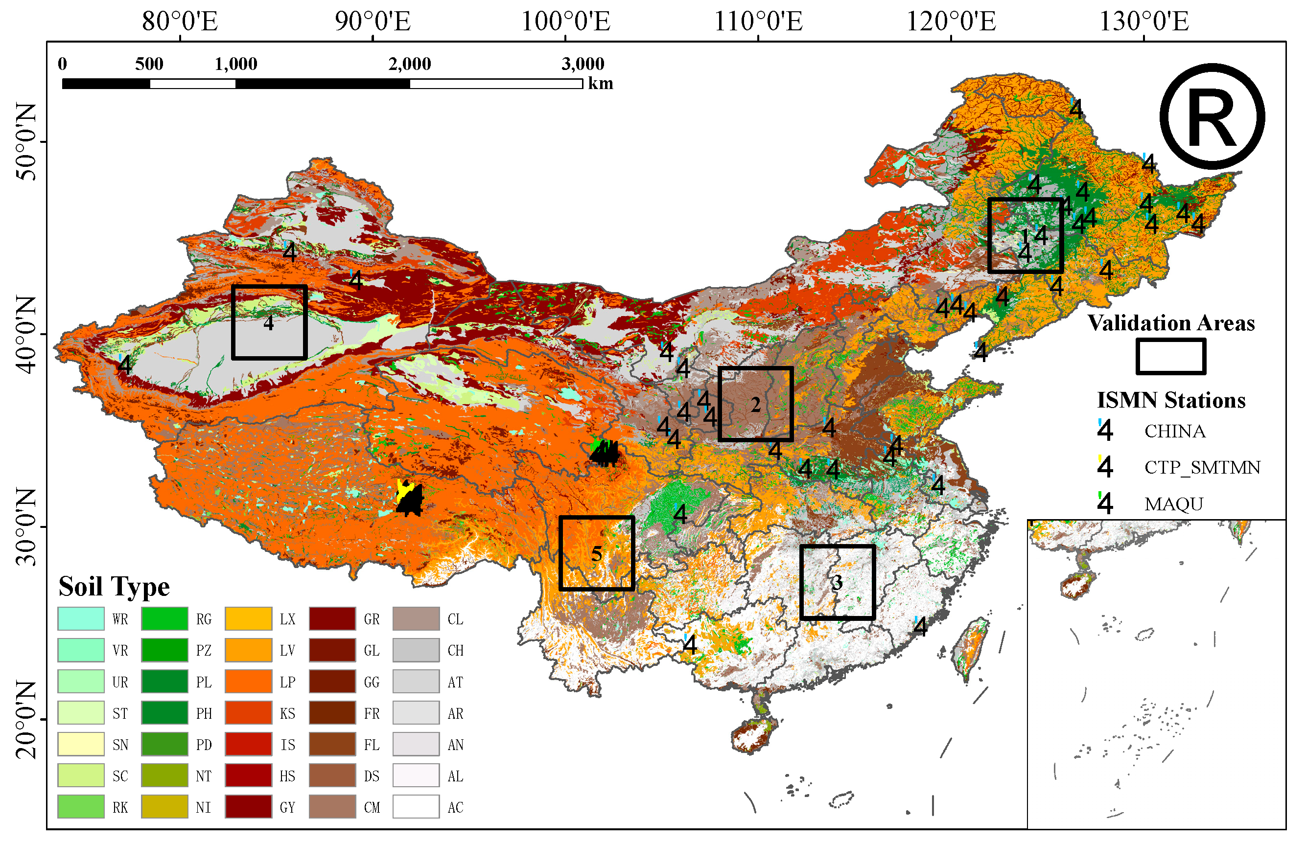
Figure 1. Spatial distribution of the study area where the background is soil type data. MAQU, CTP_SMTMN, and CHINA are three networks of in situ SM. Five black boxes are randomly selected areas for simulating data gaps. WR: Water Bodies. VR: Vertisols. UR: Urban. ST: Salt Flats. SN: Solonetz. SC: Solonchaks. RK: Rock Outcrop. RG: Regosols. PZ: Podzols. PL: Planosols. PH: Phaeozems. PD: Podzoluvisols. NT: Nitisols. NI: No Data. LX: Lixisols. LV: Luvisols. LP: Leptosols. KS: Kastanozems. IS: Island. HS: Histosols. GY: Gypsisols. GR: Greyzems. GL: Gleysols. GG: Glaciers. FR: Ferralsols. FL: Fluvisols. DS: Sand Dunes. CM: Cambisols. CL: Calcisols. CH: Chernozems. AT: Anthrosols. AR: Arenosols. AN: Andosols. AL: Alisols. AC: Acrisols.
Remotesensing 13 02848 g001
Figure 2. (a1a3) are original CCI SM in June 1990, July 2000, and August 2010, respectively; (b1b3) are gap-filled CCI SM using FNN method in those months; (c1c3) are gap-filled CCI SM using RF method in those months; (d1d3) are gap-filled CCI SM using OK method in those months; (e1e3) are gap-filled CCI SM using GLM method in those months. The white areas represent gaps of CCI SM. The color bar ranged from the lowest 0.033 to the highest 0.433.
Remotesensing 13 02848 g002aRemotesensing 13 02848 g002b
Figure 3. (a) The data gap ratios in original CCI SM and (b) the increased pixels by ML and OK gap-filling methods during the whole study period.
Remotesensing 13 02848 g003
Figure 4. Boxplots of (a) RMSE in cm3/cm3, (b) ubRMSE in cm3/cm3, (c) correlation coefficient R, and (d) BIAS in cm3/cm3 between simulated SM and original ESA CCI SM during the whole study period.
Remotesensing 13 02848 g004
Figure 5. Spatial distributions of (a) original CCI SM and simulated SM by (b) RF, (c) OK, (d) GLM, and (e) FNN methods. The first line is Region 1 in October 1979. The second line is Region 2 in October 1984. The third line is Region 3 in April 1994. The fourth line is Region 4 in August 2008. The last line is Region 5 in June 2018.
Remotesensing 13 02848 g005
Figure 6. Statistical histogram of the difference between original CCI SM and other four kinds simulated SM Deviation calculated by simulated data and ESA CCI data. Region 1–5 was symbolized by (ae) in sequence.
Remotesensing 13 02848 g006
Figure 7. Scatterplots between the gap-filled SM and the original ESA CCI SM over the five simulated data gaps. Region 1–5 was symbolized by 1–5 in sequence and FNN, GLM, OK, RF was symbolized by (ad) in sequence.
Remotesensing 13 02848 g007aRemotesensing 13 02848 g007b
Figure 8. Comparisons between in situ SM and estimated SM at each network (CHINA, CTP-SMTMN, MAQU) and all networks (ALL) with evaluation indicators of (a) RMSE, (b) ubRMSE, (c) R, and (d) BIAS.
Remotesensing 13 02848 g008
Figure 9. Comparisons of estimated SM by different strategies with the CCI SM over simulated gap areas using (a) RMSE, (b) ubRMSE, (c) R, and (d) BIAS.
Remotesensing 13 02848 g009aRemotesensing 13 02848 g009b
Figure 10. Comparisons of estimated SM by different strategies with the in situ SM using (a) RMSE, (b) ubRMSE, (c) R, and (d) BIAS.
Remotesensing 13 02848 g010
Table 1. Characters of the SM and ancillary dataset used in the study.
VariableCategoryUnitSpatial ResolutionTemporal Resolution
SMCCI SM combined v4.5m3m−30.25 degrees1 day
NDVIGIMMS NDVI
and MOD13C2
-0.083 degrees
/0.05 degrees
15 days
/monthly
PrecipitationCMDC Grided Datamm0.5 degreesmonthly
TemperatureCMDC Grided Data°C0.5 degreesmonthly
DEMGTOPO 30m0.0083 degrees-
Soil typeHarmonized World
Soil Database
-0.0083 degrees-
In situ dataInternational Soil
Moisture Network
m3m−3--
Table 2. The statistics of R, R2, RMSE, ubRMSE, and BIAS between simulated data and ESA CCI data in the 5 regions.
IndicatorsMethodRegion 1Region 2Region 3Region 4Region 5Average
RMSEFNN0.1100.0900.0770.0820.0710.086
GLM0.0570.0650.0680.0730.0800.069
OK0.0280.0380.0210.0280.0310.029
RF0.0310.0400.0260.0270.0330.031
ubRMSEFNN0.0740.0660.0420.0710.0550.062
GLM0.0490.0590.0510.0500.0750.057
OK0.0280.0360.0200.0280.0310.029
RF0.0310.0370.0220.0250.0330.029
BIASFNN−0.083−0.0610.077−0.0500.046−0.014
GLM0.030−0.0070.033−0.0480.0270.007
OK0.002−0.0130.0020.0020.001−0.001
RF5.05 × 10−5−0.0060.007−0.003−0.001−0.001
RFNN0.2030.1970.210−0.0240.5330.224
GLM0.3850.0890.0060.5020.1620.229
OK0.7970.6330.7940.8740.8630.792
RF0.7410.6120.7520.8630.8550.765
R2FNN0.0410.0390.0445.76 × 10−40.2840.083
GLM0.1480.0083.6 × 10−50.2520.0260.087
OK0.6350.4010.6300.7640.7450.635
RF0.5490.3750.5660.7450.7310.593
Publisher’s Note: MDPI stays neutral with regard to jurisdictional claims in published maps and institutional affiliations.