Article

Evaluation of Five Deep Learning Models for Crop Type Mapping Using Sentinel-2 Time Series Images with Missing Information

1
Key Laboratory of Agricultural, Institute of Agricultural Resources and Regional Planning Remote Sensing, Chinese Academy of Agricultural Sciences, Ministry of Agriculture and Rural Affairs, Beijing 100081, China
2
International Center for Tropical Agriculture (CIAT), Hanoi 100000, Vietnam
*
Author to whom correspondence should be addressed.
Remote Sens. 2021, 13(14), 2790; https://doi.org/10.3390/rs13142790
Submission received: 14 May 2021 / Revised: 2 July 2021 / Accepted: 13 July 2021 / Published: 15 July 2021
(This article belongs to the Special Issue Near Real-Time (NRT) Agriculture Monitoring)

Abstract

:
Accurate crop type maps play an important role in food security due to their widespread applicability. Optical time series data (TSD) have proven to be significant for crop type mapping. However, filling in missing information due to clouds in optical imagery is always needed, which will increase the workload and the risk of error transmission, especially for imagery with high spatial resolution. The development of optical imagery with high temporal and spatial resolution and the emergence of deep learning algorithms provide solutions to this problem. Although the one-dimensional convolutional neural network (1D CNN), long short-term memory (LSTM), and gate recurrent unit (GRU) models have been used to classify crop types in previous studies, their ability to identify crop types using optical TSD with missing information needs to be further explored due to their different mechanisms for handling invalid values in TSD. In this research, we designed two groups of experiments to explore the performances and characteristics of the 1D CNN, LSTM, GRU, LSTM-CNN, and GRU-CNN models for crop type mapping using unfilled Sentinel-2 (Sentinel-2) TSD and to discover the differences between unfilled and filled Sentinel-2 TSD based on the same algorithm. A case study was conducted in Hengshui City, China, of which 70.3% is farmland. The results showed that the 1D CNN, LSTM-CNN, and GRU-CNN models achieved acceptable classification accuracies (above 85%) using unfilled TSD, even though the total missing rate of the sample values was 43.5%; these accuracies were higher and more stable than those obtained using filled TSD. Furthermore, the models recalled more samples on crop types with small parcels when using unfilled TSD. Although LSTM and GRU models did not attain accuracies as high as the other three models using unfilled TSD, their results were almost close to those with filled TSD. This research showed that crop types could be identified by deep learning features in Sentinel-2 dense time series images with missing information due to clouds or cloud shadows randomly, which avoided spending a lot of time on missing information reconstruction.

1. Introduction

Accurate crop type information plays an important role in food security due to its widespread applicability, such as in yield estimates, crop rotation, and agricultural disaster assessment [1,2]. Optical time series data (TSD) have been proven to be efficient for crop type mapping, because the phenological evolution of each crop produces a unique temporal profile of reflectance [3]. However, filling in missing information due to clouds in optical imagery is always needed [4,5,6,7]. Although many different methods of missing information reconstruction have been developed [8,9,10], the majority of the high-precision methods are time-consuming and need a significant amount of computing resources [11], especially for images with high spatial resolution. In addition, the results with TSD after filling in missing information always include a degree of uncertainty for crop type classification.
With the launch of remote sensing satellites with sessions providing high spatial and temporal resolution optical TSD, such as Sentinel-2 with 5-day revisit intervals and 10 m spatial resolution, increasing non-cloud covered information in TSD can be used [12]. Moreover, the 13 spectrum bands of Sentinel-2 provide abundant spectral information for crop type identification using TSD with missing information; specifically, its three red-edge (RE) bands have been found to be of importance in the discrimination of different crop types due to their sensitivity to different leaf and canopy structures [13,14,15]. In addition, except for tropical or very arid regions, most crop systems have one or two (winter and summer) growing seasons each year. For example, in southern China, even in the summer growing season with more clouds and rain, very few areas are completely covered by clouds during the completely growing season [16]. Therefore, if the information that is not covered by clouds in dense Sentinel-2 TSD is fully utilized, the heavy work of missing information reconstruction and the risk of error transmission in crop type mapping may be avoided in most situations.
Deep learning provides an important solution for mining distinguishable features of different crop types from the dense TSD with missing information. In deep learning algorithms, the recurrent neural network (RNN) [17] and one-dimensional convolutional neural network (1D CNN) [18] have demonstrated excellent performance in the extraction of temporal features [19,20]. Moreover, in order to solve the problem of gradient disappearance or explosion of the RNN in increasing time series, long short-term memory (LSTM) and the gate recurrent unit (GRU) were developed [21,22]. Although the above models have been used in crop type identification [7], the potential application of CNN and RNN in optical TSD has been inadequately explored [5]. In fact, it has been proved that the RNN could use TSD with missing values for classification problems [23,24,25]. Meanwhile, the CNN can classify images with missing data via the convolution kernel operation [26,27].
At present, in the remote sensing community, the cloud pixels in optical imagery have been treated as noise in RNN models [28,29,30] or zeros in CNN models [31]. In addition, to the best of our knowledge, there is almost no research that has systematically analyzed the performance of different deep learning algorithms for crop type mapping using dense Sentinel-2 TSD with missing information to identify crop types. Therefore, in order to explore the capabilities of the CNN, LSTM, GRU, LSTM-CNN, and GRU-CNN models for crop type mapping using Sentinel-2 TSD with missing information due to clouds, we conducted two groups of experiments to address the research questions that follow:
  • What accuracies can different deep learning models achieve for crop type classification by using the Sentinel-2 TSD with missing information (unfilled TSD)?
  • Can these models achieve higher accuracies when using the Sentinel-2 TSD after filling in missing information (filled TSD) than when using unfilled TSD?

2. Materials

2.1. Study Site

Hebei Province (Figure 1) is located in North China, and Hengshui City is situated between 37°03′–38°23′ N and 115°10′–116°34′ E, covering an area of 8.12 × 10 3   km 2 (Figure 1), of which farmland occupies 5.17 × 10 3   km 2 (approx. 70.3%) [32]. Rotation of winter wheat and summer maize dominates the agricultural activities in the region, while the main economic crops are cotton, chili, common yam rhizome, fruit trees, and vegetables. The typical growing season for winter wheat is from early October to the middle of the following June, while summer maize is planted at the end of the winter wheat season and harvested in late September. The growth seasons of cotton, chili, and common yam rhizome are early April–end of October, mid-June–end of September, and mid-April–end of October, respectively. The growth periods of the fruit trees and greenhouse vegetables generally last the entire year.

2.2. Ground Reference Data

A field investigation in the study area was conducted in July 2019, when the summer crops were in their reproductive period. First, we planned the sampling route based on expert knowledge in order to collect the samples of the major crop types. Second, we traveled along the sampling route and recorded the crop types and geographic coordinates of raw samples. Ultimately, we acquired 1377 samples from the field survey. Following this, 805 samples were obtained by the manual interpretation of Google Earth Map data, and manual samples and the survey samples were located in the same parcels. Therefore, a total of 2182 sample points (Figure 1) were obtained from ground surveys for seven main types of local vegetation in the summer season: (1) greenhouse vegetables, (2) summer maize, (3) cotton, (4) chili, (5) common yam rhizome, (6) fruit trees, and (7) forests. The distribution of the number of samples per type is listed in Table 1, and the crop calendars of main crop types, i.e., summer maize, cotton, chili, and common yam rhizome, are listed in Table 2.
In Table 1, the sample size of different crop types is quite different; specifically, the sample size of summer maize is as high as 897. This is because summer maize is the main food crop in the study region with a large planting area. At the same time, considering the influence of geographical environment and other factors, we sampled summer maize more evenly along the sampling route. In Table 2, the calendars are expressed in two ways, date and day of year (DOY), to facilitate analysis.

2.3. Sentinel-2 Data and Preprocessing

Sentinel-2A/2B imagery (Level-1C) time series (with a temporal resolution of five days) were downloaded from the European Space Agency’s (ESA) Sentinel Scientific Data Hub (https://scihub.copernicus.eu/dhus/#/home). In the study area, there were 148 images (tiles T50SLG, T50SLH, T50SMG, and T50SMH) acquired from day DOY 91–273 (1 April –30 September) 2019, covering the growing seasons of the main crops. Hence, the length of the time series was 37. The satellite product is equipped with a sensor with blue, green, red, and near-infrared 1 (NIR1) bands at 10 m; RE1, RE2, RE3, NIR2, shortwave infrared 1 (SWIR1), and SWIR2 at 20 m; and three atmospheric bands at 60 m. The three atmospheric bands were not used in this paper since they are primarily dedicated to atmospheric correction and cloud screening [12]. In other words, 10 bands with resolutions of 10 m or 20 m would be used because deep learning methods could deeply extract the separable features of different crop types.
The preprocessing stages of the Sentinel-2 images included the following:
(1)
Atmospheric calibration. The Sen2Cor plugin v2.5.5 was employed to process images from top-of-atmosphere Level-1C Sentinel-2 to bottom-of-atmosphere Level-2A (http://www.esa-sen2agri.org/ (accessed on 6 April 2020)).
(2)
Masking of clouds. Fmask (Function of mask) 4.0 [33] was utilized to mask clouds and cloud shadows (the parameter of the cloud probability threshold was set as 50%). Fmask 4.0, the most recent version of Fmask [34] can work on Sentinel-2 images in Level-1C. All masks have a 20-m resolution, and both clouds and cloud shadows were marked as missing data. It should be noted that compared with cloud confidence layers in the output of Sen2Cor, most Fmask 4.0 results are more accurate in our study area.
(3)
Resampling. The images of the RE1, RE2, RE3, NIR2, SWIR1, and SWIR2 bands from step (1) and the cloud masks from step (2) were resampled to 10 m using the bilinear interpolation method [35].
Finally, we obtained the time series of samples marked with missing elements in pixel scale.

3. Methodology

3.1. LSTM and GRU for TSD with Missing Values

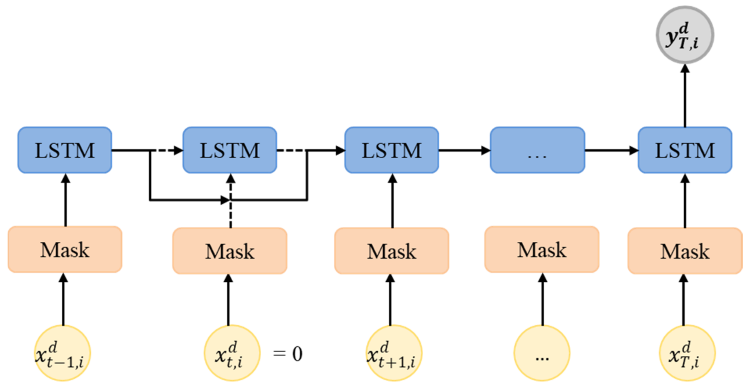
As mentioned earlier, 10 bands (variables) of Sentinel-2 images with cloud tags were used in this research, and the sequence length of these images was 37. LSTM units cannot compute null values (i.e., miss values) during the training process; as discussed in Section 1, if we set null values as zeros, the training and testing results will be highly biased. Thus, inspired by Che et al. [23], a Mask layer to overcome the problem of missing values in time series was adopted, which made the pixels covered by the cloud not participate in the calculation, and the networks were labelled as Mask LSTM RNNs. Figure 2 presents the details of the Mask layer in a Mask LSTM RNN. We express the i t h sample as X i = ( x 1 i , x 2 i , , x T i ) , where T = 37 , x t i D denotes the t t h observation of all variables, and x t i d represents the value of the d t h variable of x t i . First, for all of the samples, the missing values were set as “0”. Then, in order to keep the “0” element unchanged after normalization, channel L2 normalization (a Mask layer to overcome the problem of missing values in time series was L2-norm) was performed on the surface reflectance, as expressed in Equation (1) [36], where 2182 is the number of samples, and X t d represents the normalized vector of the d t h variable in the t t h observation. Note that the channel here is a band of Sentinel-2 data of all of the samples on an acquisition date, and in the feature vector after the L2-norm, “0” elements have not been changed. Then, when a batch of samples is input into Mask LSTM RNNs, the Mask layer will produce a mask matrix with the shape of the input data, and the values of the mask matrix can be calculated using Equation (2). When the LSTM cells find m t i d = 0 , the corresponding x t i d will be skipped, and the output of the ( t 1 ) t h LSTM unit will be delivered to the ( t + 1 ) t h LSTM unit. The detailed operations are illustrated in Equations (3)–(8), where f t + 1 , i d , p t + 1 , i d , and o t + 1 , i d are the outputs of the forget gate, input gate, and output gate of the d t h channel of the ( t + 1 ) t h LSTM unit, respectively; C is the cell memory state; C represents the update values of unit status; h is the hidden state; W and b are the corresponding weights and biases. It is worth noting that if there are two or more LSTM layers in a Mask LSTM RNN, the mask matrix will be delivered until it reaches the last LSTM layer.
X t d = ( x t 1 d 2 , x t 2 d 2 , , x t 2182 d 2 ) 1 / 2
m t i d = 1 , i f x t i d 0 0 , i f x t i d = 0
f t + 1 , i d = σ ( W f [ h t 1 , i d , x t + 1 , i d ] + b f ) ,
p t + 1 , i d = σ ( W p [ h t 1 , i d , x t + 1 , i d ] + b p ) ,
o t + 1 , i d = σ ( W o [ h t 1 , i d , x t + 1 , i d ] + b o ) ,
C t + 1 , i d = tanh ( W C [ h t 1 , i d , x t + 1 , i d ] + b C ) ,
C t + 1 , i d = f t + 1 , i d C t 1 , i d + p t + 1 , i d C t + 1 , i d
h t + 1 , i d = o t + 1 , i d tanh ( C t + 1 , i d ) .
Similarly, when the LSTM units shown in Figure 2 are replaced with GRU units [21], a Mask GRU RNN for processing TSD with missing values will be obtained.

3.2. 1D CNN for TSD with Missing Values

The 1D CNN is a special form of CNN that employs one-dimensional convolution (Conv1D) kernels (also known as filters) to capture the temporal pattern or shape of the input series [37]. Unlike LSTM and GRU models, the convolutional operation is the dot product between the filters and local regions of the input. Therefore, we express the i t h sample of the input layer as X i 0 = ( x 1 i 0 , x 2 i 0 , , x T i 0 ) . Consider that the length of the first layer convolution kernel is k; then, the output value of the first layer at time point t can be calculated using Equation (9), where conv1D (…) is a regular 1D convolution, 0 k k , and W k 1 is the weight vector. When x ( t + k k ) , i 0 = 0 , the extracted feature of the first layer x t i 1 does not contain the missing elements of the input data. Therefore, the output layer of the 1D CNN does not contain the features of elements denoted as zeros.
x t i 1 = k 1 k c o n v 1 D ( W k 1 , x ( t + k k ) , i 0 )
A rectified linear unit (ReLU) layer (also known as the activation function) always follows the Conv1D layer. In addition, it is common to incorporate other components, such as dropout [38], batch normalization (BN) [39], and the fully connected (FC) layer, [40] into CNN architectures. For classification tasks, all of the above layers followed a softmax logistic regression layer, which acts as a classifier [41,42].

3.3. Experimental Configurations

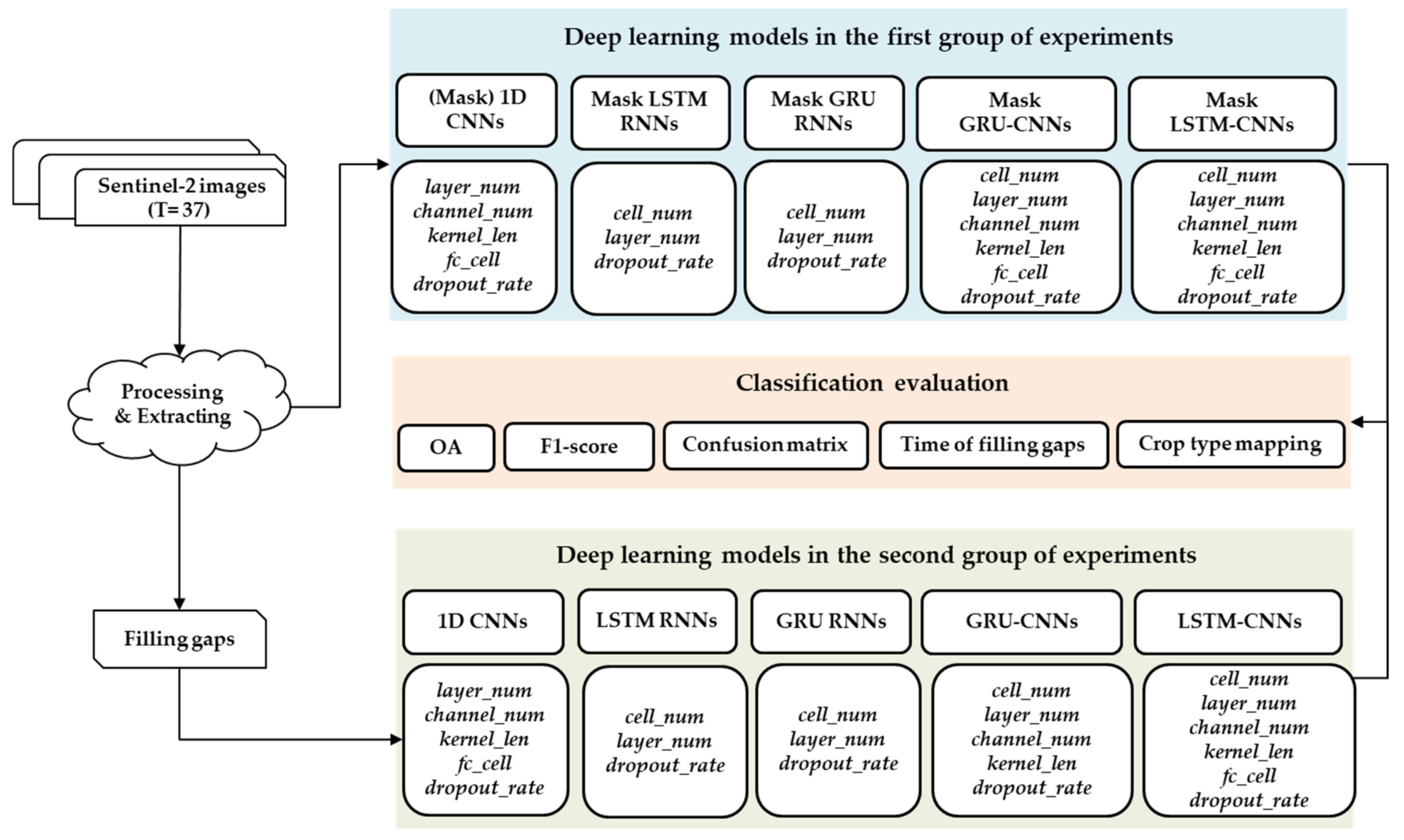
The following experiments (shown in Figure 3) were designed for the 1D CNN, LSTM, GRU, LSTM-CNN, and GRU-CNN models to address the two questions raised in Section 1. In Figure 3, the text in italics includes the hyper-parameters that need to be trained. We implemented our models using the Keras API with TensorFlow backend, using an Nvidia GeForce GTX Titan X (12-Gb RAM).
The first group of experiments was designed to answer the first question by building networks based on the five aforementioned models using unfilled TSD; and these networks were then named as (Mask) 1D CNNs, Mask LSTM RNNs, Mask GRU RNNs, Mask LSTM-CNNs, and Mask GRU-CNNs. The raw spectral information from each band of Sentinel-2 during the growing season (defined as DOY 91–273 in intervals of 5 days) was input to the training networks, and all missing elements due to clouds were set as zeros.
In the second group of experiments, filled TSD was used to build networks based on the five aforementioned models; and these networks were named as 1D CNNs, LSTM RNNs, GRU RNNs, LSTM-CNNs, and GRU-CNNs. First, we filled in missing information in TSD using time series linear interpolation based on good-quality observations, since linear interpolation is usually appropriate for TSD with short gaps [43]. The Sentinel-2 images observed in March and October 2019 were used as well because there were clouds in the images observed in early April and late September. Second, we utilized the Savitzky–Golay filter to reconstruct each band value, using a moving window of seven observations and a filter order of two [44]. Third, the spectral information of all 10 bands of the filled Sentinel-2 TSD was input to the training networks.
Experiential values and the grid search method were used together to train the hyper-parameters of all networks. For example, the experiential values of the dropout rate were 0.3, 0.5, and 0.8 [45], and the cell numbers in LSTM and GRU (module) were selected from {64,128,256,512} [7,46,47]. The training of parameters for networks was performed by using the Adam optimizer with cross entropy loss [48]; some classification tasks of TSD have demonstrated this to be successful [47,49]. In addition, we monitored each training process with the ModelCheckpoint callback function [50] and saved the model when a better model of the training set was found. For each type of network, to reduce the influence of random sample splitting bias, we repeated the random split five times, and this allowed us to compute the average performances. Moreover, for each split, we randomly selected 70% and 10% of the samples per crop type to form the training set and the validation set, respectively; the remaining samples (20%) constituted the test set since the distribution of sample sizes per crop type was uneven.
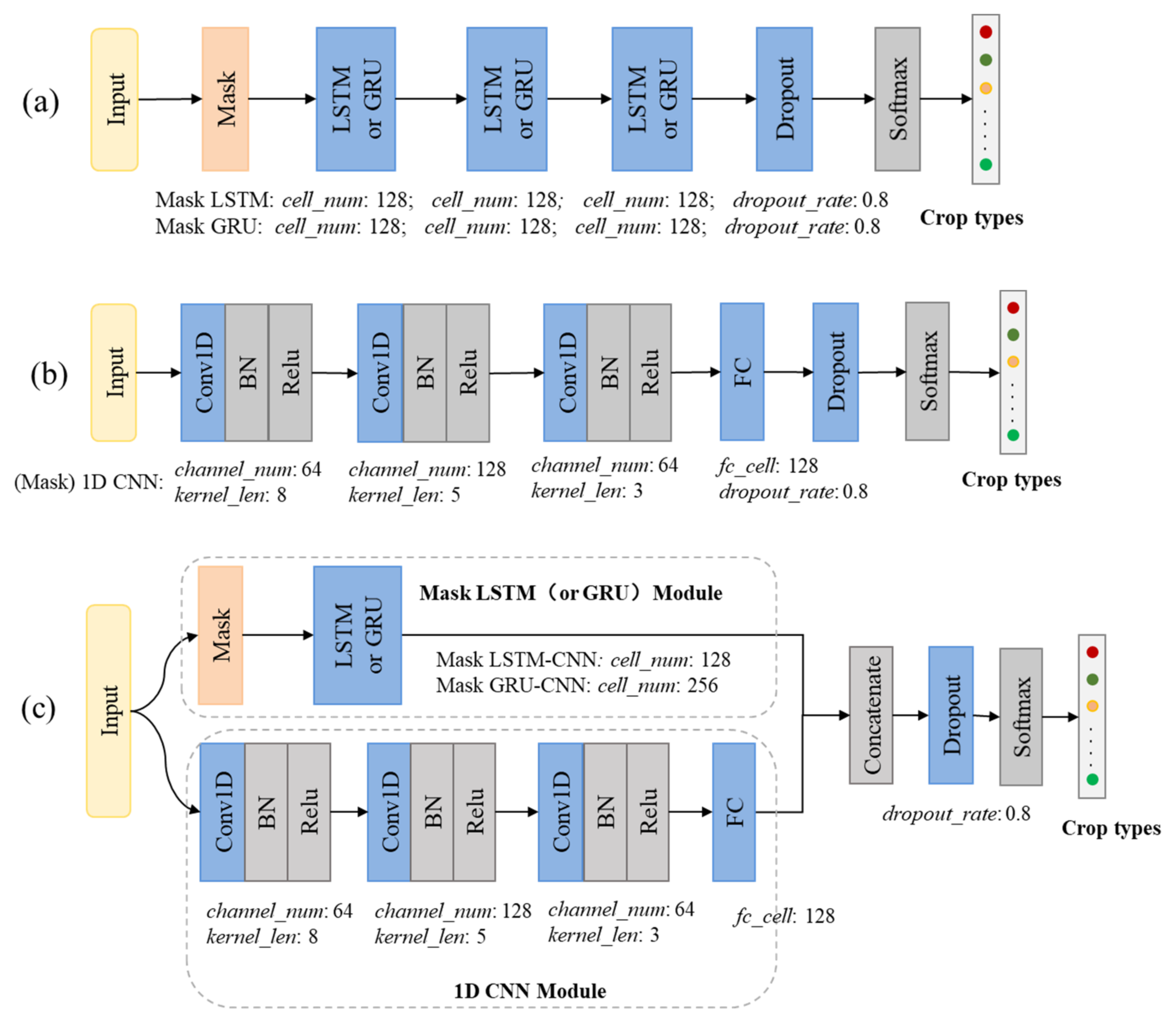
Figure 4a–c show the architectures and optimal hyper-parameter values of (Mask) 1D CNNs, Mask LSTM RNNs, Mask GRU RNNs, Mask LSTM-CNNs, and Mask GRU-CNNs obtained using unfilled TSD in the first group of experiments. In the second group of experiments, five architectures similar to those shown in Figure 4 were built, first. Then, these architectures were trained by using filled TSD since the number of features and the temporal length of the input data in the two groups were the same. Finally, we obtained the architectures and optimal hyper-parameters of 1D CNNs, LSMT RNNs, GRU RNNs, LSMT-CNNs, and GRU-CNNs. There were two main differences between these networks in the second group and those shown in Figure 4. First, the number of channels of the three convolutional layers of 1D CNN were 128,256, and 128, respectively. Second, there were no mask layers in LSMT RNNs, GRU RNNs, and LSMT (and GRU) modules of LSMT-CNNs and GRU-CNNs.

3.4. Evaluation Methods

Except for the confusion matrices of the test set, the accuracy of crop type classification was evaluated in terms of overall accuracy (OA) [51]. The accuracy of each crop type was assessed using the F1 score (F1), which is the harmonic mean of precision and recall [52]. In order to evaluate the stability of different models, for each type of networks, we calculated the standard deviations of OA and F1 of the networks upon application to five test sets. Moreover, we calculated the time spent to fill in missing information of Sentinel-2 time series data covering a typical mapping region in the study area to evaluate the efficiency of crop type mapping using unfilled TSD.

4. Results

4.1. Unfilled and Filled Sentinel-2 TSD

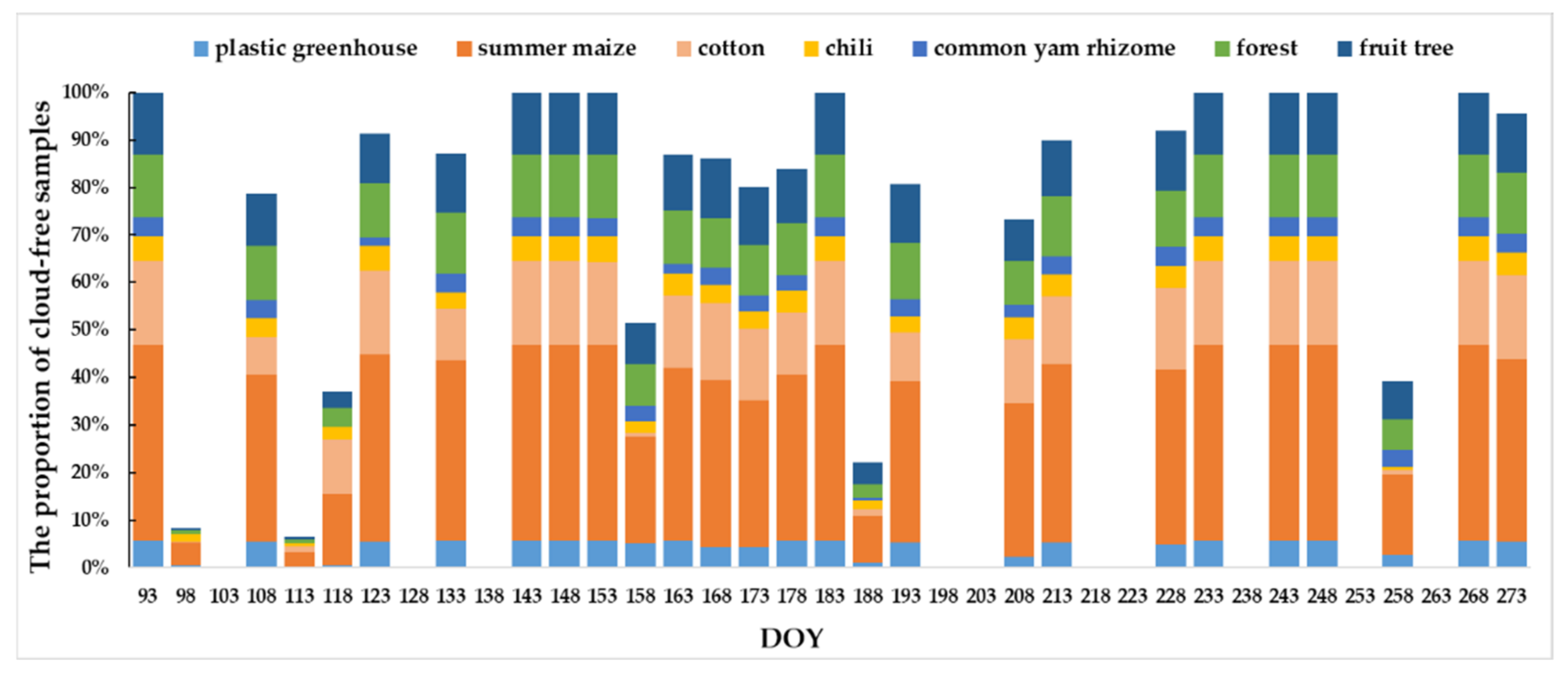
The proportions of cloud-free samples in Hengshui City from 1 April to 30 September 2019 are shown in Figure 5 to illustrate the number of missing values in TSD. In Figure 5, the x-axis is the DOY when the Sentinel-2 imagery was acquired, the y-axis is the accumulated proportion of samples for each crop type that was not covered by clouds or cloud shadows, and each color represents a crop type. Throughout the growth season, there were 10 dates when the values of all samples were missing, and only nine dates when the proportion of cloud-free samples was 100%; on the other 18 dates, a part of the samples was covered. Statistics revealed that the total missing rate of sample values was 43.5%.
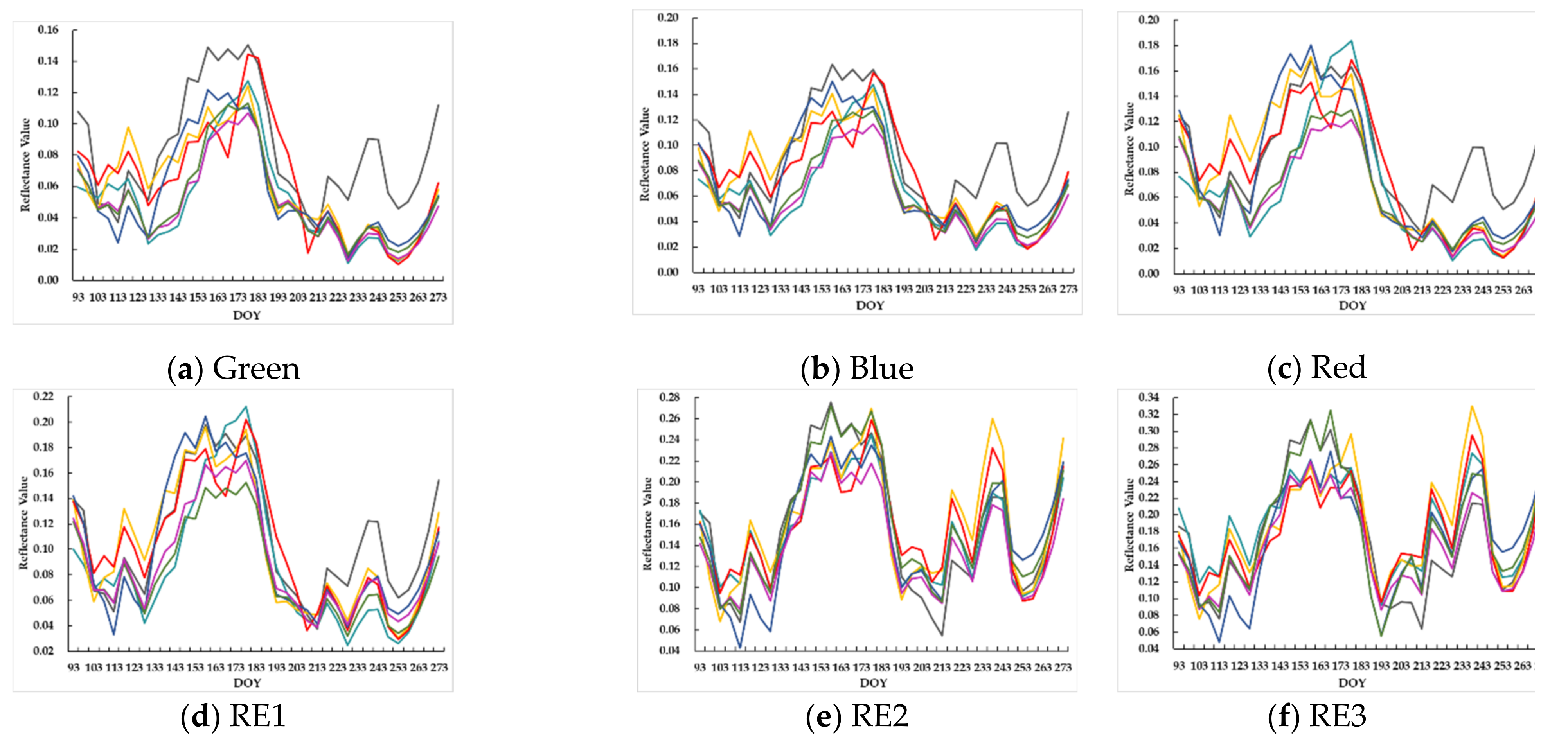
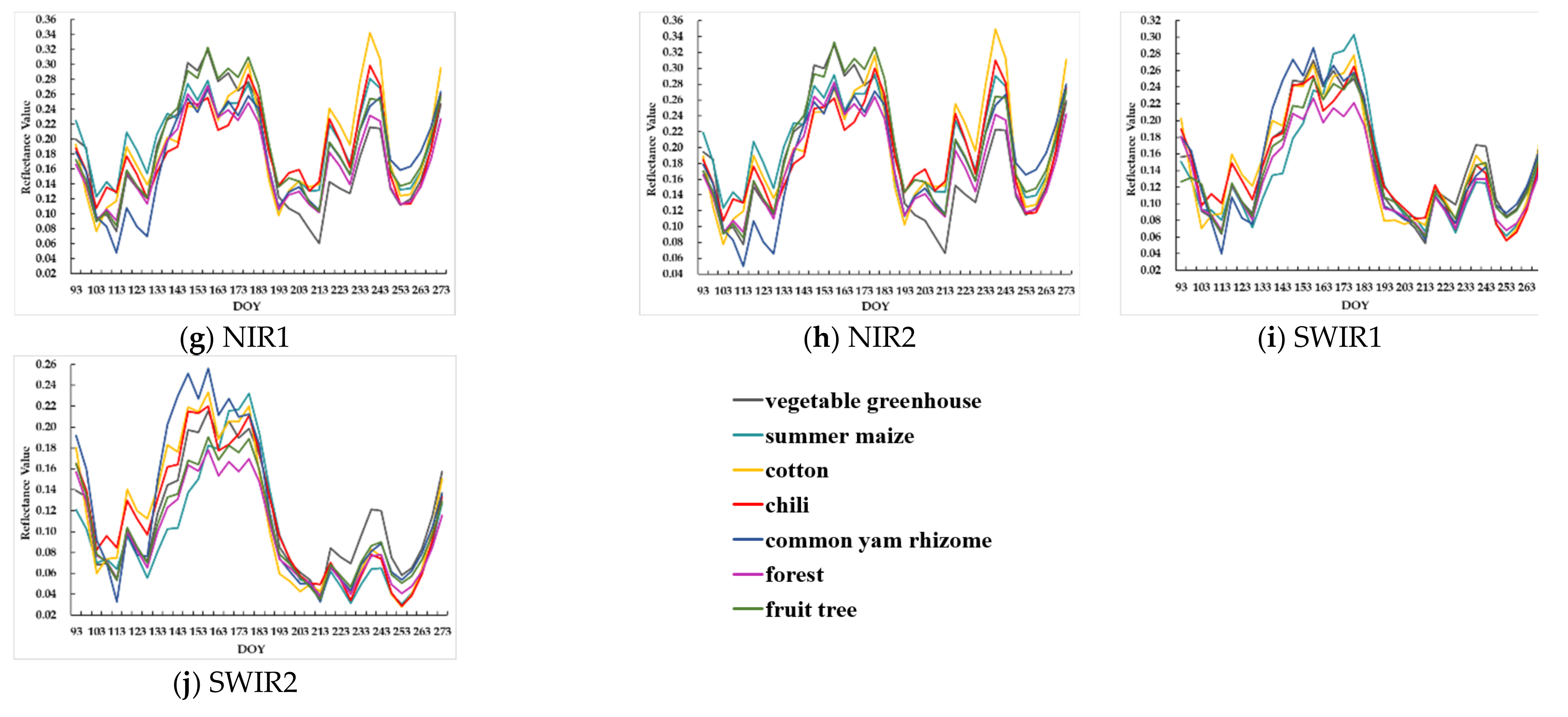
The missing elements of samples in the TSD were filled in using time series linear interpolation and Savitzky–Golay smoothing. The average bottom-of-atmosphere reflectance profiles of each crop type are shown in Figure 6, which illustrates the potential of filled TSD for contributing to crop type classification. In Figure 6, the x-axis is the DOY, and the y-axis is the average bottom-of-atmosphere reflectance value of samples per type.
For the visible spectral bands shown in Figure 6a–c, the reflectance curves of the different crop types exhibited obvious differences from DOY 93–183 and more intersections and overlaps after DOY 183 (i.e., early July) because they were all in the developing period, resulting in similar features in the visible spectra. For the RE1–RE3 bands, the reflectance curves of RE1 were similar to those of the red bands, and RE2 and RE3 displayed more similarity with each other. Compared with NIR1 and NIR2, which had very similar reflectance curves for the same crop type, the SWIR1 and SWIR2 profiles exhibited larger differences. In addition, similar to the visible spectra, the SWIR1 and SWIR2 profiles of all of the vegetation types were very close after DOY 183. Overall, these results showed that RE2–3 and NIR1–2 spectra were valuable for crop type classifications in the study area. It should be noted that since the width of the vegetable greenhouse is generally 5–6 m and the resolution of Sentinel-2 is 10 m, the spectra of the vegetable greenhouse samples were similar to those of other vegetation due to mixture pixels.

4.2. Classification Accuracy with Unfilled TSD

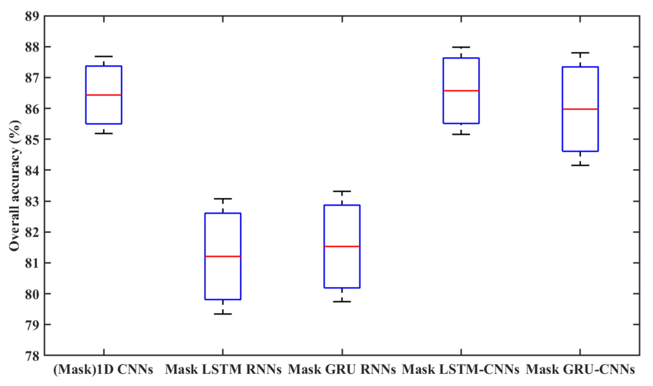
Figure 7 shows the average OAs and standard deviations of different networks over five different random splits in the first group of experiments using unfilled TSD. First, we found that Mask LSTM-CNNs achieved the highest average OA (86.57%), improving by 0.14% from (Mask) 1D CNNs; meanwhile, the average OA of Mask GRU-CNNs was 85.98%, which was worse than that of (Mask) 1D CNNs. Second, Mask LSTM RNNs attained the lowest average OA (81.21%), while Mask GRU RNNs achieved the second lowest average OA. Therefore, from the perspective of OA, 1D CNN, LSTM-CNN, and GRU-CNN could extract more discriminative features from unfilled TSD than LSMT and GRU. From the perspective of the stability of different networks, (Mask) 1D CNNs attained the lowest OA standard deviation over five different random splits, indicating that 1D CNN was the most stable model for crop type classification using unfilled TSD, followed by LSTM-CNN.
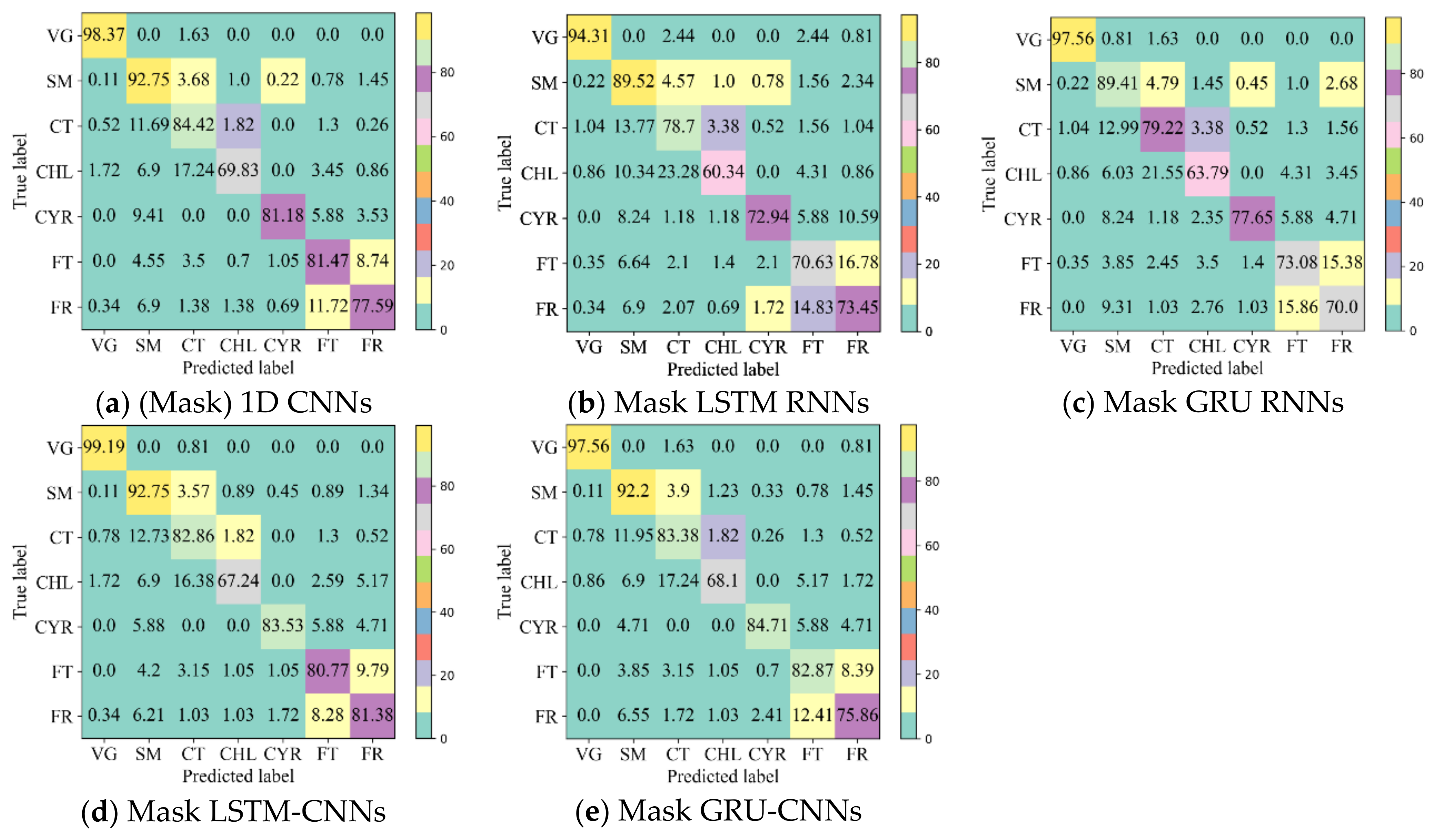
Figure 8a–e show confusion matrices of the networks based on five deep learning models using unfilled TSD. The values in the matrices are the percentage of points available in the “true label” and are the averages of the five test sets, that is, the values on the principal diagonal are the recalls of crop types [53]. First, the recalls of vegetable greenhouse were almost above 95% with different networks due to the non-vegetation characteristics of the greenhouse. Second, fruit tree and forest were easily confused with each other; for example, Mask LSTM-CNNs, which best distinguished them, inadvertently classified 9.79% of fruit trees as forests and 8.28% of forests as fruit trees. The main reason can be gleamed from Figure 6; the overlap ratio of the Sentinel-2 multi-spectral reflectance curves of the two types is very high. These two situations belong to non-crop monitoring and different “forest” land classification, respectively. Next, we discuss the other four crop types.
The confusion matrices obtained by different networks had similar performances on the other four crop types. First, cotton and common yam rhizome were most likely to be inadvertently classified as summer maize, and chili was more likely to be inadvertently classified as common yam rhizome. These results can be explained by the reflectance curves shown in Figure 6; chili and common yam rhizome show obvious discrepancies on the visible spectra and RE1 spectrum, but their reflectance curves are very close on other spectra. This illustrates that the missing values in the Sentinel-2 TSD did not affect the distinguishable characteristics across crop types. Besides, Mask LSTM-CNNs and Mask GRU-CNNs achieved higher recalls on common yam rhizome with 85 samples than other networks, which indicated that the networks of hybrid models attained high recalls for the crop type with a small sample size using unfilled TSD.
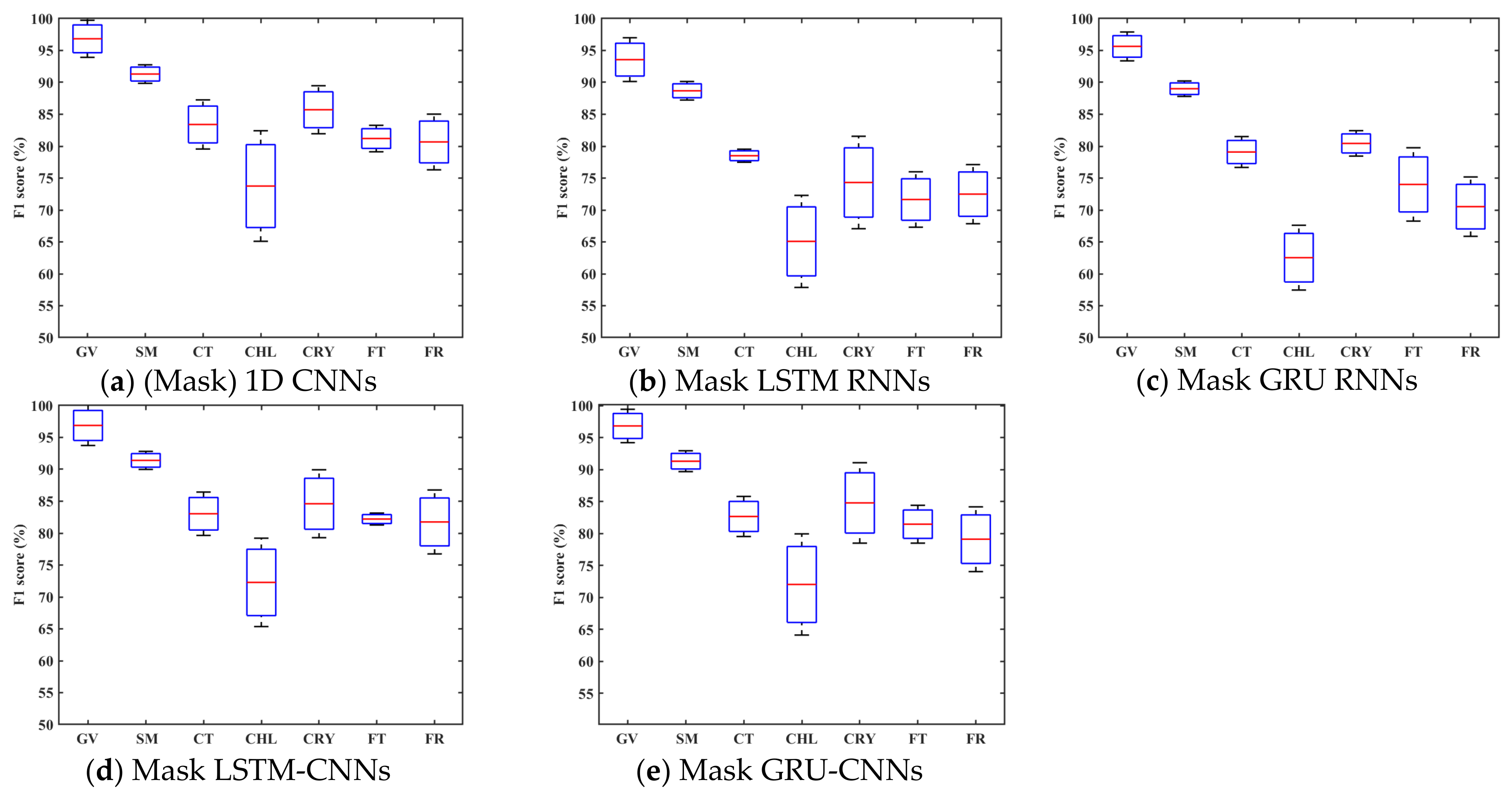
This study used F1, the harmonic mean of precision and recall, to explore the performances of different networks per crop type. The F1 results of experiments using unfilled TSD are shown in Figure 9 alongside the average F1s and standard deviations from application to the five test sets.
It is to be noted that (Mask) 1D CNNs achieved the highest average F1s on cotton, chili, and common yam rhizome; conversely, Mask LSTM-CNNs achieved the highest average F1s on vegetable greenhouse, summer maize, fruit tree, and forest. These results illustrate that these two types of networks had different advantages in the detection of different crop types in the study area, even though their OAs are very close. However, for summer maize and vegetable greenhouse, both networks achieved high F1s (above 90%) due to the non-vegetation characteristics of vegetable greenhouses (as discussed above) and the large area of summer maize parcels. At the same time, we found that all five types of networks achieved the lowest average F1s on chili. This is mainly because the chili parcels in the study area were always smaller than the spatial resolution of 10 m, resulting in mixed pixels. From the perspective of the stability of different networks on crop type detection, all five types of networks attained the smallest F1 standard deviations on summer maize, larger F1 standard deviations on cotton and common yam rhizome, and the largest F1 standard deviations on chili. The above-mentioned mixed pixels were one of the factors that caused these phenomena. In addition, a large sample size of the crop type was beneficial to the stability of the deep learning models.

4.3. Comparison of Classification Accuracy with Filled and Unfilled TSD

Table 3 shows the average OAs and standard deviations of five deep learning models using unfilled TSD in the first group and filled TSD in the second group, calculated over five random split test sets. The 1D CNN, LSTM-CNN, and GRU-CNN all had acceptable average OAs (above 85%) with filled TSD and unfilled TSD; meanwhile, LSMT and GRU attained lower OAs with filled TSD and unfilled TSD. In addition, the OAs of these models in different groups were close. These results indicated that the five models could deep learn features of different crop types from Sentinel-2 dense TSD with missing information, even though the missing rate of Sentinel-2 TSD of all of the samples was 43.5%. Moreover, we found that the standard deviations of each model using filled TSD were larger than those using unfilled TSD, which was mainly caused by the transfer error of interpolation and smoothing methods.
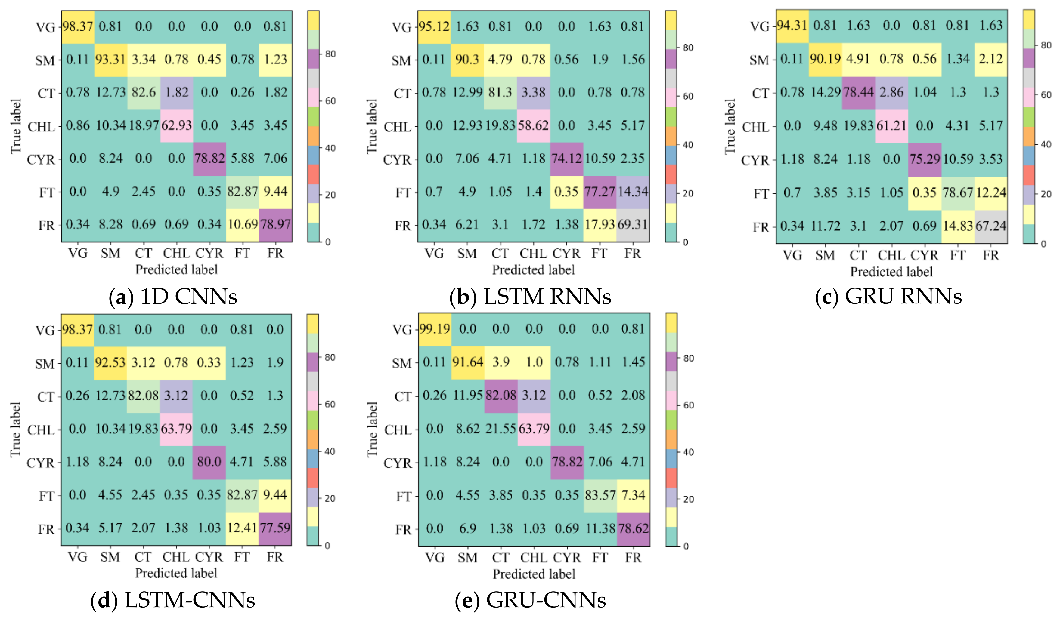
The average confusion matrices of the five test sets obtained by the different deep learning models using filled TSD are shown in Figure 10. As stated in Section 4.2, the values in the matrices are the percentage of points available in the “true label diagonal,” and the values on the principal are recalls. First, we found that the ability of each model to distinguish between every pairing of crop types when using filled TSD is similar to that when using unfilled TSD. For example, common yam rhizome and cotton were easily classified as summer maize in both groups. This indicates that the missing values caused by clouds did not reduce the separability between different crop types because the low proportion of cloud-free samples (Figure 5) were mainly on the dates when the reflectance profiles of different crop types were close (Figure 6). The recalls of cotton, chili, and common yam rhizome shown in Figure 10 are smaller than those shown in Figure 8. For example, the maximum recall of common yam rhizome is 80.0% in Figure 10 but 84.71% in Figure 8. This indicates that filling in missing values may reduce the recalls of the crop types with mixed pixels due to smaller parcels.
The average F1s and standard deviations of each crop type attained by the five deep learning models using unfilled TSD and filled TSD are shown in Table 4. The mask networks used unfilled TSD in the first group of experiments, and the other networks used filled TSD in the second group of experiments. The values in bold are the higher average F1s per crop type between results of different networks based on the same model. Obviously, except for LSTM, the other four models obtained higher F1s when using unfilled TSD than when using filled TSD. In addition, the F1 standard deviations of different crop types using unfilled TSD are similar to those using filled TSD. For example, in both groups, all five models achieved small F1 standard deviations on summer maize and large F1 standard deviations on chili.

4.4. Crop Type Mapping

Since the reconstruction of missing values in long-term series is a time-consuming task, we selected a typical region (Figure 11a) in the study area, over which summer maize, cotton, chili, common yam rhizome, and fruit tree/forest were mapped, and two non-vegetation masks were used. The first one was the NIR1 reflectance image (without clouds) attained on 21 August 2019, because the NIR spectrum showed great potential in discriminating between vegetation and non-vegetation [54,55]. The NIR1 reflectance of vegetation was above 0.31, which was obtained by subtracting the mean standard deviation from the mean value of vegetation land cover (cropland and natural vegetation). In addition, because of the obvious non-vegetation characteristics of greenhouses, the buildings and roads in the farmland can be easily inadvertently classified as vegetable greenhouses. Therefore, we used the results of vegetable greenhouse as another non-vegetation mask to supplement the first one.
In the first group of experiments, the crop type mapping results of the five deep learning models using unfilled TSD are shown in Figure 11b–f, covering a region with 329,181 pixels. First, we found that there are similar crop type distributions in the maps of (b) (mask) 1D CNNs, (e) mask LSTM-CNNs, and (f) mask GRU-CNNs. Moreover, there are more common yam rhizome pixels in (e) and (f), which is consistent with the conclusion obtained in Section 4.2, i.e., compared with (mask) 1D CNNs, the hybrid networks achieved higher recalls for crop types with small sample sizes or small parcels.
In the second group of experiments, we first used linear interpolation and the Savitzky–Golay filter to fill in the missing values of the regional time series images, which took 61.3 min. The computing environment was the Windows 10 OS on a PC with a dual-core processor (@2.10 GHz) and 64 GB memory. The mapping results of the five models using the reconstructed TSD are shown in Figure 11g–k. By comparing the mapping results of the five models in the two groups, we found that there are more cotton, chili, and common yam in Figure 11b,e,f than in Figure 11g 1D CNNs, (j) LSTM-CNNs, and (k) GRU-CNNs. This is consistent with the conclusion in Section 4.3, i.e., filling in missing values may reduce the recalls of crop types with mixed pixels due to smaller parcels.

5. Discussion

5.1. Performances of Different Models

We summarize the performance of the five deep learning models in the following three points.
(1)
The 1D CNN has the potential to learn highly discriminative features for crop type mapping by using TSD with missing information. First, it achieved acceptable accuracy (above 85%) using unfilled TSD; moreover, its OA was higher and performances more stable than those with filled TSD. Second, it attained higher F1s on different crop types when using unfilled TSD than when using filled TSD, especially on cotton, chili, and common yam rhizome, which could easily be inadvertently classified. Third, it had higher recalls on cotton, chili, and common yam rhizome when using unfilled TSD than when using filled TSD (see Figure 11, which illustrates that the interpolated and smoothed TSD may reduce the recalls of crop types with small parcels). Although LSTM and GRU did not attain accuracies as high as 1D CNN using unfilled TSD, their results were almost close to those with filled TSD.
(2)
In the two groups of experiments, the performance of LSTM-CNN and GRU-CNN was similar to that of 1D CNN (as discussed in (1)). However, in the mapping results using unfilled TSD, their recall rates of chili and common yam rhizome with small samples and small parcels were higher than that of 1D CNN. This showed that for crop type identification using TSD with missing information, the hybrid model of CNN and RNN (LSTM or GRU) has more advantages than a single model.
(3)
When using the networks in the second group for crop type mapping, we first filled in the missing values in the time series images of the mapping area. In this study, there were 329,181 pixels in the mapping area (shown in Figure 11a), and it took 61.3 min to fill in gaps. If we map the crop types of the entire Hengshui City ( 8.12 × 10 3   km 2 ) and use a computer (configured as stated in Section 4.4) to fill in the missing values, it will take about 11.5 days. This is very detrimental to the efficiency of crop monitoring over large areas. Therefore, we believe that this study is of great significance for improving the efficiency of crop monitoring over large areas.

5.2. Limitations

It is worth noting that there are some limitations and uncertainties in this study. The first one is that in the study area (Hengshui City, located in northern China), the missing rate of Sentinel-2 values of samples was approximately 43.5%, and the low proportion of cloud-free samples (Figure 5) were mainly on the dates when the reflectance profiles of different crop types were close to each other (see Figure 6). In contrast, rainy weather and cloud cover are frequent in southern China, and as much as 80% of the Sentinel-2 images of that region acquired throughout the year may include clouds (note that 80% is not the percentage of cloud coverage) [49]. In this case, the networks based on the above deep learning models may fail for crop type detection using TSD with missing values because the missing information are more easily on the key dates for distinguishing close reflectance profiles of crop types. Therefore, the reduction of the cost of missing information reconstruction through deep learning methods for crop type mapping in cloudy and rainy areas will be the focus of our future work.
In addition, this study used linear interpolation and the Savitzky–Golay filter to fill in the missing information of time series images; these are currently widely employed in crop type classification based on dense TSD and deep learning methods [4,5,6,7]. However, some gap-filling methods achieve higher precision by collaboratively using temporal, spatial, or spectrum information [11], although they will require more time and computing resources than those employed in the present study. Therefore, the second group of experiments using filled TSD achieved lower accuracies, which might relate to the missing information reconstruction method we adopted. This work needs to be further verified in the future.

6. Conclusions

Cropland is the most complex land-use type since both human activity and the natural environment affect it. Deep learning methods could identify crop types by learning these complex relationships in depth. However, we often need to reconstruct the missing values in the remote-sensed optical imagery due to clouds, which increases the workload and the risk of error transmission. In this paper, we explored the performance of five deep learning models (i.e., the 1D CNN, LSTM, GRU, LSTM-CNN, and GRU-CNN) for crop type mapping using Sentinel-2 (Sentinel-2) time series data (TSD) with missing information. The results show that although the total missing rate of the sample TSD was approximately 43.5%, the 1D CNN, LSTM-CNN, and GRU-CNN all achieved acceptable classification accuracy (above 85%). Moreover, when compared with using filled TSD, they recalled more samples on crop types with small parcels than when using unfilled TSD. Although LSTM and GRU did not attain accuracies as high as the other three models using unfilled TSD, their results were almost close to those with filled TSD. This study is important for both scientific and practical uses, although it has some limitations and uncertainties, as stated in Section 5.2. It showed that crop types could be identified by deep learning features in Sentinel-2 dense time series images with missing information due to clouds or cloud shadows randomly, which avoided spending extra time on missing information reconstruction. In the future, the networks can be extended to two dimensions to complete the semantic segmentation of time series images with missing values.

Author Contributions

H.Z. carried out the evaluations and analysis, and wrote the original draft; H.Z. and L.S. designed the schemes; H.Z. and J.L. led the main work in this study; S.D. and L.S. offered many valuable comments and considerations; L.R. provided several opinions, constructive suggestions and discussions. All of the authors have read and agreed to the final version of the manuscript.

Funding

This research was supported by the Monitoring and Forecasting of Crop Growth and Productivity Based on Satellite Remote Sensing Data (Grant No. 2016YFD0300603), the Fundamental Research Funds for Central Non-profit Scientific Institution (Grant Nos. 1610132021021 and 1610132020017), and the National Natural Science Foundation of China (Grant No. 41921001).

Institutional Review Board Statement

The study was conducted according to the guidelines of the Declaration of Helsinki, and approved by the Institutional Review Board (or Ethics Committee) of NAME OF INSTITUTE (protocol code XXX and date of approval).

Informed Consent Statement

Informed consent was obtained from all subjects involved in the study.

Conflicts of Interest

The authors declare no conflict of interest.

References

  1. Kogan, F.; Kussul, N.N.; Adamenko, T.I.; Skakun, S.V.; Kravchenko, A.N.; Krivobok, A.A.; Shelestov, A.Y.; Kolotii, A.V.; Kussul, O.M.; Lavrenyuk, A.N. Winter wheat yield forecasting: A comparative analysis of results of regression and bio-physical models. J. Autom. Inf. Sci. 2013, 45, 68–81. [Google Scholar] [CrossRef]
  2. Kolotii, A.; Kussul, N.; Shelestov, A.; Skakun, S.; Yailymov, B.; Basarab, R.; Lavreniuk, M.; Oliinyk, T.; Ostapenko, V. Comparison of biophysical and satellite predictors for wheat yield forecasting in Ukraine. ISPRS Int. Arch. Photogramm. Remote Sens. Spat. Inf. Sci. 2015, XL-7/W3, 39–44. [Google Scholar] [CrossRef] [Green Version]
  3. Wardlow, B.D.; Egbert, S.L.; Kastens, J.H. Analysis of time-series MODIS 250m vegetation index data for crop classification in the U.S. Central Great Plains. Remote Sens. Environ. 2007, 108, 290–310. [Google Scholar] [CrossRef] [Green Version]
  4. Cai, Y.; Guan, K.; Peng, J.; Wang, S.; Seifert, C.; Wardlow, B.; Li, Z. A high-performance and in-season classification system of field-level crop types using time-series Landsat data and a machine learning approach. Remote Sens. Environ. 2018, 210, 35–47. [Google Scholar] [CrossRef]
  5. Pelletier, C.; Webb, G.I.; Petitjean, F. Temporal Convolutional Neural Network for the Classification of Satellite Image Time Series. Remote Sens. 2019, 11, 523. [Google Scholar] [CrossRef] [Green Version]
  6. Xu, J.; Zhu, Y.; Zhong, R.; Lin, Z.; Lin, T. Deep Crop Mapping: A multi-temporal deep learning approach with improved spa-tial generalizability for dynamic corn and soybean mapping. Remote Sens. Environ. 2020, 247, 111946. [Google Scholar] [CrossRef]
  7. Zhong, L.; Hu, L.; Zhou, H. Deep learning based multi-temporal crop classification. Remote Sens. Environ. 2019, 221, 430–443. [Google Scholar] [CrossRef]
  8. Ng, M.K.-P.; Yuan, Q.; Yan, L.; Sun, J. An Adaptive Weighted Tensor Completion Method for the Recovery of Remote Sensing Images With Missing Data. IEEE Trans. Geosci. Remote Sens. 2017, 55, 3367–3381. [Google Scholar] [CrossRef]
  9. Sun, L.; Chen, Z.; Gao, F.; Anderson, M.; Song, L.; Wang, L.; Hu, B.; Yang, Y. Reconstructing daily clear-sky land surface temperature for cloudy regions from MODIS data. Comput. Geosci. 2017, 105, 10–20. [Google Scholar] [CrossRef]
  10. Tang, Z.; Adhikari, H.; Pellikka, P.K.; Heiskanen, J. A method for predicting large-area missing observations in Landsat time series using spectral-temporal metrics. Int. J. Appl. Earth Obs. Geoinf. 2021, 99, 102319. [Google Scholar] [CrossRef]
  11. Shen, H.; Li, X.; Cheng, Q.; Zeng, C.; Yang, G.; Li, H.; Zhang, L. Missing Information Reconstruction of Remote Sensing Data: A Technical Review. IEEE Geosci. Remote Sens. Mag. 2015, 3, 61–85. [Google Scholar] [CrossRef]
  12. Drusch, M.; Bello, U.D.; Carlier, S.; Colin, O.; Fernandez, V.; Gascon, F.; Hoersch, B.; Isola, C.; Laberinti, P.; Martimort, P. Sentinel-2: ESA’s Optical High-Resolution Mission for GMES Operational Services. Remote Sens. Environ. 2012, 120, 25–36. [Google Scholar] [CrossRef]
  13. Vuolo, F.; Neuwirth, M.; Immitzer, M.; Atzberger, C.; Ng, W.-T. How much does multi-temporal Sentinel-2 data improve crop type classification? Int. J. Appl. Earth Obs. Geoinf. 2018, 72, 122–130. [Google Scholar] [CrossRef]
  14. Lambert, M.-J.; Traoré, P.C.S.; Blaes, X.; Baret, P.; Defourny, P. Estimating smallholder crops production at village level from Sentinel-2 time series in Mali’s cotton belt. Remote Sens. Environ. 2018, 216, 647–657. [Google Scholar] [CrossRef]
  15. Ustuner, M.; Sanli, F.B.; Abdikan, S.; Esetlili, M.T.; Kurucu, Y. Crop Type Classification Using Vegetation Indices of RapidEye Imagery. ISPRS Int. Arch. Photogramm. Remote Sens. Spat. Inf. Sci. 2014, XL-7, 195–198. [Google Scholar] [CrossRef] [Green Version]
  16. Sun, L.; Xia, X.; Wang, P.; Fei, Y. Do aerosols impact ground observation of total cloud cover over the North China Plain? Glob. Planet. Chang. 2014, 117, 91–95. [Google Scholar] [CrossRef]
  17. Werbos, P. Backpropagation through Time: What It Does and How to Do It; Institute of Electrical and Electronics Engineers (IEEE): Piscataway Township, NJ, USA, 1990; Volume 78, pp. 1550–1560. [Google Scholar]
  18. Wang, Z.; Yan, W.; Oates, T. Time series classification from scratch with deep neural networks: A strong baseline. In Proceedings of the 2017 International Joint Conference on Neural Networks (IJCNN), Anchorage, AK, USA, 14–19 May 2017; pp. 1578–1585. [Google Scholar]
  19. Fawaz, H.I.; Forestier, G.; Weber, J.; Idoumghar, L.; Muller, P. Deep learning for time series classification: A review. Data Min. Knowl. Discov. 2019, 33, 917–963. [Google Scholar] [CrossRef] [Green Version]
  20. Zheng, Y.; Liu, Q.; Chen, E.; Ge, Y.; Zhao, J.L. Time Series Classification Using Multi-Channels Deep Convolutional Neural Networks; Li, F., Li, G., Hwang, S., Yao, B., Zhang, Z., Eds.; Web-Age Information Management; Springer: Cham, Switzerland, 2014; pp. 298–310. [Google Scholar]
  21. Cho, K.; Van Merrienboer, B.; Bahdanau, D.; Bengio, Y. On the Properties of Neural Machine Translation: Encoder–Decoder Approaches; Association for Computational Linguistics (ACL): Baltimore, MA, USA, 2014. [Google Scholar]
  22. Hochreiter, S.; Schmidhuber, J. Long short-term memory. Neural Comput. 1997, 9, 1735–1780. [Google Scholar] [CrossRef] [PubMed]
  23. Che, Z.; Purushotham, S.; Cho, K.; Sontag, D.; Liu, Y. Recurrent Neural Networks for Multivariate Time Series with Missing Values. Sci. Rep. 2018, 8, 1–12. [Google Scholar] [CrossRef] [Green Version]
  24. Parveen, S.; Green, P. Speech Recognition with Missing Data using Recurrent Neural Nets. In Proceedings of the Neural In-formation Processing Systems, Vancouver, BC, Canada, 3–8 December 2001; pp. 1189–1195. [Google Scholar]
  25. Tian, Y.; Zhang, K.; Li, J.; Lin, X.; Yang, B. LSTM-based traffic flow prediction with missing data. Neurocomputing 2018, 318, 297–305. [Google Scholar] [CrossRef]
  26. Cao, K.; Kim, H.; Hwang, C.; Jung, H. CNN-LSTM Coupled Model for Prediction of Waterworks Operation Data. J. Inf. Process. Syst. 2018, 14, 1508–1520. [Google Scholar]
  27. Eitel, A.; Springenberg, J.T.; Spinello, L.; Riedmiller, M.; Burgard, W. Multimodal deep learning for robust RGB-D object recognition. In 2015 IEEE/RSJ International Conference on Intelligent Robots and Systems (IROS); IEEE: Piscataway Township, NJ, USA, 2015; pp. 681–687. [Google Scholar]
  28. Mazzia, V.; Khaliq, A.; Chiaberge, M. Improvement in Land Cover and Crop Classification based on Temporal Features Learning from Sentinel-2 Data Using Recurrent-Convolutional Neural Network (R-CNN). Appl. Sci. 2019, 10, 238. [Google Scholar] [CrossRef] [Green Version]
  29. Rußwurm, M.; Körner, M. Temporal Vegetation Modelling using Long Short-Term Memory Networks for Crop Identification from Medium-Resolution Multi-Spectral Satellite Images. In Proceedings of the IEEE Conference on Computer Vision and Pattern Recognition, Honolulu, HI, USA, 21–26 July 2017; pp. 1496–1504. [Google Scholar]
  30. Rußwurm, M.; Körner, M. Multi-Temporal Land Cover Classification with Sequential Recurrent Encoders. ISPRS Int. J. Geo-Inf. 2018, 7, 129. [Google Scholar] [CrossRef] [Green Version]
  31. Sharma, A.; Liu, X.; Yang, X. Land cover classification from multi-temporal, multi-spectral remotely sensed imagery using patch-based recurrent neural networks. Neural Netw. 2018, 105, 346–355. [Google Scholar] [CrossRef] [PubMed] [Green Version]
  32. Liu, H.; Guo, H.; Yang, L.; Wu, L.; Li, F.; Li, S.; Ni, P.; Liang, X. Occurrence and formation of high fluoride groundwater in the Hengshui area of the North China Plain. Environ. Earth Sci. 2015, 74, 2329–2340. [Google Scholar] [CrossRef]
  33. Qiu, S.; Zhu, Z.; He, B. Fmask 4.0: Improved cloud and cloud shadow detection in Landsats 4–8 and Sentinel-2 imagery. Remote Sens. Environ. 2019, 231, 111205. [Google Scholar] [CrossRef]
  34. Zhu, Z.; Woodcock, C.E. Object-based cloud and cloud shadow detection in Landsat imagery. Remote Sens. Environ. 2012, 118, 83–94. [Google Scholar] [CrossRef]
  35. Onojeghuo, A.O.; Blackburn, G.A.; Wang, Q.; Atkinson, P.; Kindred, D.; Miao, Y. Mapping paddy rice fields by applying machine learning algorithms to multi-temporal Sentinel-1A and Landsat data. Int. J. Remote Sens. 2018, 39, 1042–1067. [Google Scholar] [CrossRef] [Green Version]
  36. Dai, Z.; Heckel, R. Channel Normalization in Convolutional Neural Network avoids Vanishing Gradients. arXiv 2020, arXiv:1907.09539. [Google Scholar]
  37. Hu, W.; Huang, Y.; Wei, L.; Zhang, F.; Li, H.-C. Deep Convolutional Neural Networks for Hyperspectral Image Classification. J. Sens. 2015, 2015, 1–12. [Google Scholar] [CrossRef] [Green Version]
  38. Hinton, G.E.; Srivastava, N.; Krizhevsky, A.; Sutskever, I.; Salakhutdinov, R. Improving neural networks by preventing co-adaptation of feature detectors. Neural Evol. Comput. 2012. [Google Scholar] [CrossRef]
  39. Ioffe, S.; Szegedy, C. Batch Normalization: Accelerating Deep Network Training by Reducing Internal Covariate Shift. Int. Conf. Mach. Learn. 2015, 37, 448–456. [Google Scholar]
  40. Boureau, Y.L.; Ponce, J.; LeCun, Y. A Theoretical Analysis of Feature Pooling in Visual Recognition. In Proceedings of the 27th international conference on machine learning (ICML-10), Haifa, Israel, 21–24 June 2010; pp. 111–118. [Google Scholar]
  41. Krizhevsky, A.; Sutskever, I.; Hinton, G.E. Imagenet classification with deep convolutional neural networks. Adv. Neural Inf. Process. Syst. 2012, 25, 1097–1105. [Google Scholar] [CrossRef]
  42. Zeiler, M.D.; Fergus, R. Stochastic Pooling for Regularization of Deep Convolutional Neural Networks. Learning 2013. [Google Scholar] [CrossRef] [Green Version]
  43. Kandasamy, S.; Baret, F.; Verger, A.; Neveux, P.; Weiss, M. A comparison of methods for smoothing and gap filling time series of remote sensing observations—Application to MODIS LAI products. Biogeosciences. 2013, 10, 4055–4071. [Google Scholar] [CrossRef] [Green Version]
  44. Chen, J.; Jonsson, P.; Tamura, M.; Gu, Z.; Matsushita, B.; Eklundh, L. A simple method for reconstructing a high-quality NDVI time-series data set based on the Savitzky–Golay filter. Remote Sens. Environ. 2004, 91, 332–344. [Google Scholar] [CrossRef]
  45. Srivastava, N.; Hinton, G.; Krizhevsky, A.; Sutskever, I.; Salakhutdinov, R. Dropout: A Simple Way to Prevent Neural Networks from Overfitting. J. Mach. Learn. Res. 2014, 15, 1929–1958. [Google Scholar]
  46. Mou, L.; Ghamisi, P.; Zhu, X.X. Deep Recurrent Neural Networks for Hyperspectral Image Classification. IEEE Trans. Geosci. Remote Sens. 2017, 55, 3639–3655. [Google Scholar] [CrossRef] [Green Version]
  47. Karim, F.; Majumdar, S.; Darabi, H.; Harford, S. Multivariate LSTM-FCNs for time series classification. Neural Netw. 2019, 116, 237–245. [Google Scholar] [CrossRef] [Green Version]
  48. Zhang, Z.; Sabuncu, M. Generalized cross entropy loss for training deep neural networks with noisy labels. In Proceedings of the Advances in Neural Information Processing Systems, Montréal, QC, Canada, 3–8 December 2018; pp. 8778–8788. [Google Scholar]
  49. Zhao, H.; Chen, Z.; Jiang, H.; Jing, W.; Sun, L.; Feng, M. Evaluation of Three Deep Learning Models for Early Crop Classifi-cation Using Sentinel-1A Imagery Time Series—A Case Study in Zhanjiang, China. Remote Sens. 2019, 11, 2673. [Google Scholar] [CrossRef] [Green Version]
  50. Lu, L.; Meng, X.; Mao, Z.; Karniadakis, G.E. DeepXDE: A Deep Learning Library for Solving Differential Equations. SIAM Rev. 2021, 63, 208–228. [Google Scholar] [CrossRef]
  51. Congalton, R.G. A review of assessing the accuracy of classifications of remotely sensed data. Remote Sens. Environ. 1991, 37, 35–46. [Google Scholar] [CrossRef]
  52. Sasaki, Y. The truth of the F-measure. Teach Tutor Mater 2007, 1, 1–5. [Google Scholar]
  53. Du, Z.; Yang, J.; Ou, C.; Zhang, T. Smallholder Crop Area Mapped with a Semantic Segmentation Deep Learning Method. Remote Sens. 2019, 11, 888. [Google Scholar] [CrossRef] [Green Version]
  54. Hao, P.; Tang, H.; Chen, Z.; Liu, Z. Early-season crop mapping using improved artificial immune network (IAIN) and Sentinel data. PeerJ 2018, 6, e5431. [Google Scholar] [CrossRef]
  55. Zhu, Z.; Woodcock, C.E. Continuous change detection and classification of land cover using all available Landsat data. Remote Sens. Environ. 2014, 144, 152–171. [Google Scholar] [CrossRef] [Green Version]
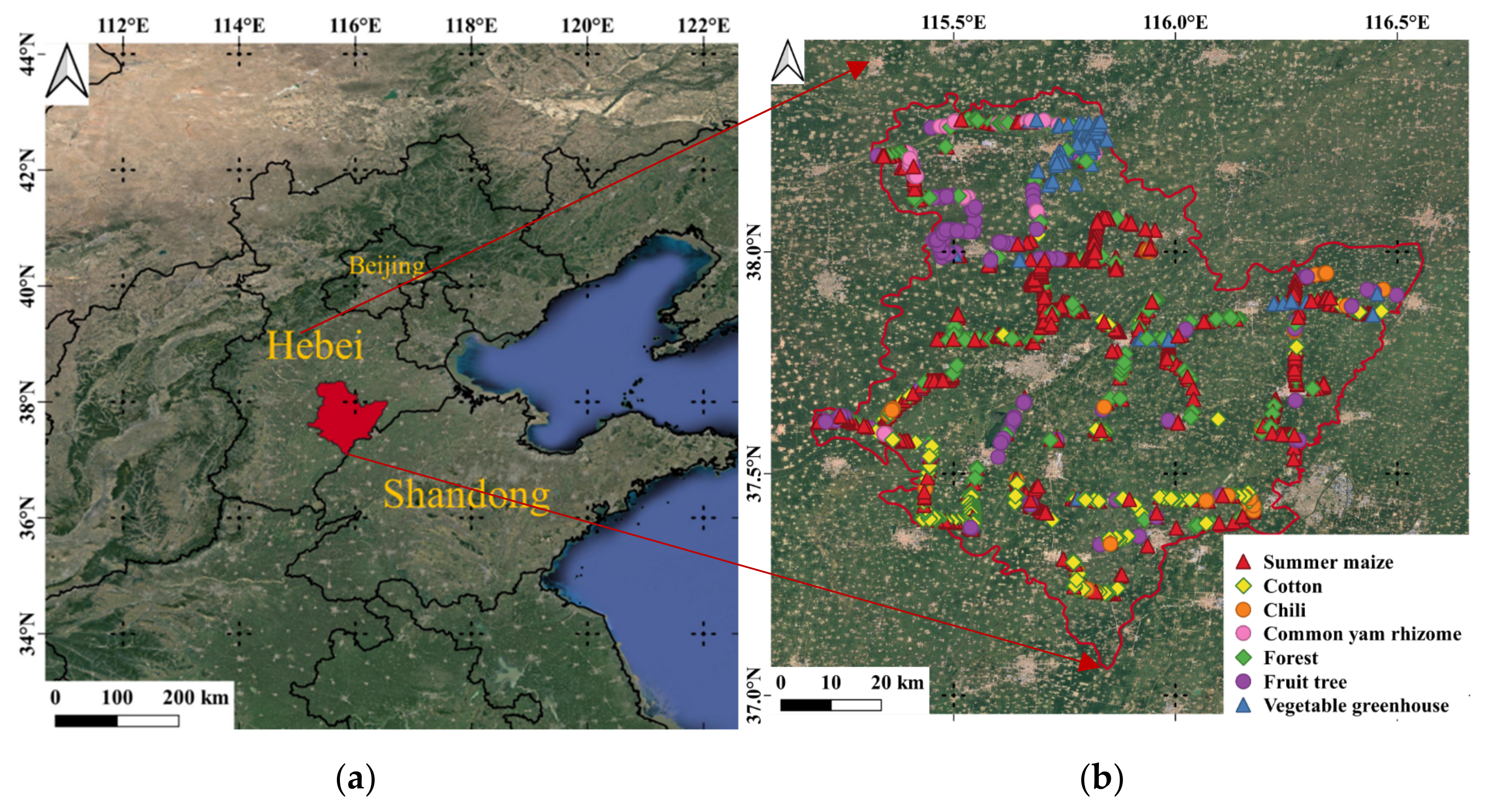
Figure 1. The study area and sample distribution: (a) Hebei Province; (b) Samples in Hengshui.
Remotesensing 13 02790 g001
Figure 2. A masked long short-term memory recurrent neural network (mask LSTM RNN) for multiple variables. LSTM, long short-term memory.
Remotesensing 13 02790 g002
Figure 3. Experimental configurations of five deep learning models using unfilled Sentinel-2 time series data in the first group of experiments and using filled Sentinel-2 time series data in the second group of experiments. T, the length of Sentinel-2 time series data. layer_num, the number of layers; channel_num, the number of channels in a convolutional layer; kernel_len, the length of kernels in a convolution layer; fc_num, the cell number of a fully connected layer; dropout_rate, the dropout rate; cell_num, the number of LSTM or GRU units in a layer. 1D CNNs, one-dimensional convolutional neural networks; RNNs, recurrent neural networks; LSTM, long short-term memory; GRU, the gate recurrent unit; OA, overall accuracy.
Remotesensing 13 02790 g003
Figure 4. Networks in the first group using unfilled Sentinel-2 time series data. (a) Mask LSTM RNNs and Mask GRU RNNs; (b) (Mask) 1D CNNs; and (c) Mask LSTM-CNNs and Mask GRU-CNNs. channel_num, the number of channels in a convolutional layer; kernel_len, the length of kernels in a convolution layer; dropout_rate, the dropout rate; cell_num, the number of LSTM or GRU units in a layer; BN, batch normalization; FC, fully connected; Conv1D, one-dimensional convolution.
Remotesensing 13 02790 g004
Figure 5. Proportions of cloud-free samples.
Remotesensing 13 02790 g005
Figure 6. (aj) Bottom-of-atmosphere reflectance profiles of each crop type from the filled Sentinel-2 time series data.
Remotesensing 13 02790 g006aRemotesensing 13 02790 g006b
Figure 7. Average overall accuracies and standard deviations (over five different random splits) of five deep learning models using unfilled Sentinel-2 time series data.
Remotesensing 13 02790 g007
Figure 8. (ae) Confusion matrices of different networks using unfilled Sentinel-2 time series data. Values in matrices are the percentage of points available in the “true label” and are the averages of the five test sets. VG, vegetable greenhouse; SM, summer maize; CT, cotton; CHL, chili; CYR, common yam rhizome; FT, fruit trees; FR, forests.
Remotesensing 13 02790 g008
Figure 9. (ae) The average F1 scores and standard deviations (from five split test sets) of each crop type with five types of networks using unfilled Sentinel-2 time series data. VG, vegetable greenhouse; SM, summer maize; CT, cotton; CHL, chili; CYR, common yam rhizome; FT, fruit trees; FR, forests.
Remotesensing 13 02790 g009
Figure 10. (ae) Confusion matrices of different networks using filled Sentinel-2 time series data. Values in matrices are the percentage of points available in the “true label” and are the average of the five test sets. VG, vegetable greenhouse; SM, summer maize; CT, cotton; CHL, chili; CYR, common yam rhizome; FT, fruit trees; FR, forests.
Remotesensing 13 02790 g010
Figure 11. The crop type maps attained by the five deep learning models. (bf) are the results with unfilled Sentinel-2 time series data; (gk) are the results with filled Sentinel-2 time series data.
Remotesensing 13 02790 g011
Table 1. Number of samples per type.
Class Label1234567Total
Class TypeGreenhouse
Vegetables
Summer
Maize
CottonChiliCommon
Yam Rhizome
Fruit
Trees
Forests
Number123897385116852862902182
Table 2. Crop calendars of summer maize, cotton, chili, and common yam rhizome in Hengshui, China. DOY, day of year.
Class TypeSowingDevelopingMaturation
DateDOYDateDOYDateDOY
Summer maizeJune 15–30166–181July 1–September 15182–259September 16–30260–274
CottonApril 1–15 91–106April 16–August 31107–244September 1–October 31245–305
ChiliJune 15–25166–176June 26–August 31177–244September 1–30245–274
Common yam rhizomeApril 1–1591–106April 16–October 10 107–284October 11–31285–305
Table 3. Average overall accuracies and standard deviations (over five different random splits) of five deep learning models using Sentinel-2 TSD with missing information and filled Sentinel-2 TSD. SD, standard deviation.
Model1D CNNLSTMGRULSTM-LSTMGRU-CNN
Networks(Mask) 1D CNNs1D CNNsMask LSTM RNNsLSTM RNNsMask GRU RNNsGRU RNNsMask LSTM-CNNsLSTM -CNNsMask GRU-CNNsGRU-CNNs
OA86.4386.2580.5782.1881.5381.6786.5785.7585.9885.61
SD1.252.621.872.841.791.871.412.261.822.32
Table 4. Average F1 scores and standard deviations (over five different random splits) per crop type attained by the five deep learning models using unfilled Sentinel-2 time series data (the “Mask” networks) and filled Sentinel-2 time series data; the values in bold are the higher average F1s per crop type based on the same model. VG, vegetable greenhouse; SM, summer maize; CT, cotton; CHL, chili; CYR, common yam rhizome; FT, fruit trees; FR, forests.
Model1D CNNLSTMGRULSTM-CNNGRU-CNN
Networks(Mask) 1D CNNs1D CNNsMask LSTM RNNsLSTM RNNsMask GRU RNNsGRU RNNsMask LSTM-CNNsLSTM-CNNsMask GRU-CNNsGRU-CNNs
VG96.83 ± 2.9196.81 ± 0.9493.57 ± 3.4394.76 ± 3.2995.64 ± 2.2693.92 ± 3.4596.88 ± 3.1497.63 ± 2.2796.81 ± 2.6198.41 ± 1.45
SM91.31 ± 1.4690.94 ± 1.3988.68 ± 1.4589.43 ± 1.4689.01 ± 1.2188.68 ± 1.6591.40 ± 1.4191.02 ± 0.7091.29 ± 1.6390.59 ± 1.44
CT83.40 ± 3.8583.25 ± 5.4678.51 ± 1.0280.11 ± 5.7579.09 ± 2.4277.90 ± 3.4083.04 ± 3.4082.56 ± 5.6482.65 ± 3.1481.38 ± 5.74
CHL73.75 ± 8.6671.28 ± 5.6665.08 ± 7.2163.52 ± 5.8162.53 ± 5.0866.97 ± 7.4672.28 ± 6.9369.13 ± 4.6772.01 ± 7.9268.86 ± 5.05
CYR85.71 ± 3.7684.84 ± 3.9574.31 ± 7.2479.67 ± 2.9880.43 ± 1.9979.05 ± 5.1584.60 ± 5.3285.03 ± 3.3684.76 ± 6.2982.73 ± 3.96
FT81.20 ± 2.0783.11 ± 5.0871.64 ± 4.3474.53 ± 5.5674.00 ± 5.7576.86 ± 4.4482.21 ± 0.9381.64 ± 4.7781.44 ± 2.9682.46 ± 4.09
FR80.66 ± 4.3779.58 ± 6.7072.48 ± 4.6371.80 ± 7.0070.53 ± 4.6569.92 ± 5.7081.75 ± 5.0178.58 ± 6.3779.09 ± 5.0680.31 ± 5.87
Publisher’s Note: MDPI stays neutral with regard to jurisdictional claims in published maps and institutional affiliations.