Article

Estimation of Heavy Metals in Agricultural Soils Using Vis-NIR Spectroscopy with Fractional-Order Derivative and Generalized Regression Neural Network

1
College of Geo-Exploration Science and Technology, Jilin University, Changchun 130026, China
2
The 10th Geological Brigade Co., Ltd. of Liaoning Province, Fushun 113004, China
*
Author to whom correspondence should be addressed.
Remote Sens. 2021, 13(14), 2718; https://doi.org/10.3390/rs13142718
Submission received: 28 May 2021 / Revised: 30 June 2021 / Accepted: 7 July 2021 / Published: 10 July 2021
(This article belongs to the Special Issue Monitoring Soil Degradation by Remote Sensing)

Abstract

:
With the development of industrialization and urbanization, heavy metal contamination in agricultural soils tends to accumulate rapidly and harm human health. Visible and near-infrared (Vis-NIR) spectroscopy provides the feasibility of fast monitoring of the variation of heavy metals. This study explored the potential of fractional-order derivative (FOD), the optimal band combination algorithm and different mathematical models in estimating soil heavy metals with Vis-NIR spectroscopy. A total of 80 soil samples were collected from an agriculture area in Suzi river basin, Liaoning Province, China. The spectra for mercury (Hg), chromium (Cr), and copper (Cu) of the samples were obtained in the laboratory. For spectral preprocessing, FODs were allowed to vary from 0 to 2 with an increment of 0.2 at each step, and the optimal band combination algorithm was applied to the spectra after FOD. Then, four mathematical models, namely, partial least squares regression (PLSR), adaptive neural fuzzy inference system (ANFIS), random forest (RF) and generalized regression neural network (GRNN), were used to estimate the concentration of Hg, Cr and Cu. Results showed that high-order FOD had an excellent effect in highlighting hidden information and separating minor absorbing peaks, and the optimal band combination algorithm could remove the influence of spectral noise caused by high-order FOD. The incorporation of the optimal band combination algorithm and FOD is able to further mine spectral information. Furthermore, GRNN made an obvious improvement to the estimation accuracy of all studied heavy metals compared to ANFIS, PLSR, and RF. In summary, our results provided more feasibility for the rapid estimation of Hg, Cr, Cu and other heavy metal pollution areas in agricultural soils.

Graphical Abstract

1. Introduction

Soil contamination has increased significantly worldwide with the rapid development of industrialization and urbanization [1,2,3]. Due to their contamination being covert, persistent and irreversible, heavy metals are among the most hazardous contamination types that threaten the health of animals and human beings throughout the food chain [4,5,6,7,8]. Soil heavy metals, especially mercury (Hg), chromium (Cr), lead (Pb), cadmium (Cd) and copper (Cu), tend to be accumulated in soils because of anthropogenic activities and their own easy migration properties as common industrial pollutants [9,10,11,12,13,14]. Thus, it is crucial to closely monitor the concentration of heavy metals. However, the mechanisms of soil evolution are complex and difficult to understand [15], and the soil properties may vary obviously on a small scale [16]. Traditional field sampling is always accompanied by sample preparation and chemical analysis, which is difficult to apply widely [17]. Alternatively, because of its low cost and environmental friendliness, visible and near-infrared (Vis-NIR) spectroscopy has been used as a viable alternative to laboratory analysis methods for soil quality assessment [18,19,20,21].
Affected by measuring environment, instrument errors or other reasons, spectra always obtain undesired side effects, such as spectral noises, baseline shift, and mixed overlapping peaks [20,22]. Spectral preprocessing techniques are utilized to reduce undesirable effects and accentuate spectral features [21]. Spectral derivatives are able to eliminate baseline drift and separate overlapping spectra, thereby turning into a frequently used spectral preprocessing technique. The positive effect of first derivatives and second derivatives on heavy metal concentration estimation has been validated and reviewed by researchers [20,23,24,25]. Nevertheless, integer derivatives disregard the gradual variation in the spectrum in slit and curvature, which leads to the loss of subtle information. Fractional-order derivative (FOD) can refine the order of conventional derivatives. Until now, researchers only applied FOD to Vis-NIR spectroscopy estimation of Pb, Zn and Cr [26,27], and the effect of FOD on other heavy metals that tend to accumulate in soils has not been reported. In addition, as a key spectral preprocessing technique, spectral dimensionality reduction can reduce data redundancy and improve the accuracy of estimation [28]. The optimal band combination algorithm can find the most suitable bands and generate an optimal combination through magnifying the correlation between dependent and independent variables [23,29]. The algorithm has been proved to be able to effectively eliminate the noise caused by second derivative [23], whereas the improvement to FOD produced by the algorithm has not been explored yet.
Other than spectral preprocessing techniques, mathematical models also have great impacts on the Vis-NIR spectroscopy estimation of soil heavy metals [30]. Commonly used mathematical models include multiple linear regression (MLR) [31], partial least squares regression (PLSR) [32], random forest (RF) [27], support vector machine (SVM) [33], and adaptive neural fuzzy inference system (ANFIS) [34]. In previous studies, ANFIS and RF reported that they performed better than other models [27,34,35]. As a kind of radial basis function neural network, the generalized regression neural network (GRNN) has excellent performance in anti-interference, the ability of autonomous learning and fast convergence speed [36]. In other applications of mathematical models, it has been proved that GRNN can achieve similar or better performance compared with RF and ANFIS [37,38,39,40]. However, there is no study comparing the performance of GRNN, ANFIS, and RF in Vis-NIR spectroscopy estimation of heavy metals in soils.
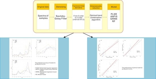
The aim of the study was to explore the potential of using appropriate preprocessing techniques and mathematical models to improve Vis-NIR spectroscopy estimation accuracy of heavy metals in soils. Hence, we introduced FOD to highlight the hidden information of the spectrum, and assessed the effect of optimal band combination algorithm on FOD. PLSR, GRNN, ANFIS and RF were utilized to estimate the concentration of Hg, Cr and Cu in soils with the spectral indices produced by the optimal band combination algorithm. Additionally, the performances of the four mathematical models were compared in detail.

2. Materials and Methods

2.1. Study Area and Sample Collection

The study area is located in the Suzi river basin, Fu Shun city, Liaoning Province, northeast China, as shown in Figure 1a. The river basin covers an area of 2161 km2, and its terrain is relatively undulating. Its climate is classified as continental monsoonal, with large temperature difference. The average annual precipitation and temperature are 759.1 mm and 5.1 °C, correspondingly. The accumulated sunshine hours in the area are between 2280 h and 2670 h, and the frost-free period is approximately 120 to 160 days. The soil types in the region include Cumulic Anthrosols, Gleyic Luvisols, Haplic Luvisols and Haplic Phaeozems [41]. The cultivated area accounts for about 13.05% of the study area, mostly distributed on both sides of the river. In this area, the crop types include rice, vegetables, and other economic crops. The upper reaches of the river basin are rich in mineral resources, with many small mines. Part of the mine tailings ponds are not designed according to standards, which leads to the leakage of heavy metal elements, thereby possibly leading to heavy metal accumulation in soils.
Sampling campaigns were carried out in October 2013, and 80 surface soil samples (0–20 cm) were collected in the study area. The coordinates of the samples sites were recorded through a handheld global positioning system, as shown in Figure 1b. Sampling points were randomly set in the cultivated lands along the river. Each sample contained five mixed subsamples, and non-soil materials were removed during collection. All samples were sealed in plastic bags and transported to the laboratory. After the samples were air-dried, the soil samples were passed through a 2 mm sieve. Each sample was divided into two parts: one part was used for spectral measurements, and the other was used for property analysis.

2.2. Chemical Analysis and Statistic

The concentration of Cr and Cu in the soil samples was measured through inductively coupled plasma atomic emission spectroscopy according to HJ 781-2016, and atomic fluorescence spectrometry was used to determine the concentration of Hg. For different heavy metal elements, the concentration was arranged in ascending order. The training set and validation set were separated as follows: the second value was selected, and then one value was selected every three values as the validation, and the remaining values were used as the training set. Each metal element was divided into a training set and validation set in a 3:1 ratio according to the method. The training set includes 60 samples, and the validation set includes 20 samples.

2.3. Spectral Measurement and Pretreatment

Spectral measurements of soil were performed with an ASD FieldSpec® 3 field spectroradiometer (Analytical Spectral Devices, Inc., Boulder, CO, USA). The device has a spectral resolution of 3 nm over the 350–1000 nm region and 10 nm over the 1000–2500 nm region, and records reflectance at 1 nm intervals. Spectral measurements were conducted in a dark room. The soil samples were uniformly put into black containers with a diameter of 10 cm, and the surface of soil samples was scraped flat. A 50 W halogen lamp was used as the light source, and the incident angle was 30°. The optical fiber probe was perpendicular to the surface of each sample at a distance of 5 cm. Before spectral measurements, the device was preheated for 30 min and optimized with a white panel. After every 10 soil samples, the whiteboard calibration was also carried out. Each sample was tested ten times, and the average value was obtained as the actual spectral reflection data.
After spectral measurements, the original spectra were treated by using the Savitzky–Golay filter [42]. A low order and narrow window size make the smoothing less effective, whereas a high order and loose window size can cause the over-smoothing phenomenon [21]. It is necessary to select moderate parameters, thus the second order and a window size of 11 points were determined [23]. After applying the Savitzky–Golay filter, marginal bands were eliminated, and the region of 400–2400 nm was used for subsequent analysis.

2.4. Spectral Feature Reduction

Vis-NIR spectroscopy data have a lot of redundant information when predicting a certain metal element in soils [43]. To avoid the situation of “dimensionality disaster”, dimensionality reduction and optimal band combination have been widely used in predicting various elements in soils [29,44,45,46,47,48,49,50]. In the study, five types of two-band spectral index are used to explore the suitable band combination for Hg, Cr, and Cu. The spectral indices include ratio index (RI), normalized difference index (NDI), difference index (DI), product index (PI), and sum index (SI). In the subsequent analyses, the five spectral indices were calculated in the training set for the optimal band combination algorithm. Additionally, the five spectral indices were calculated in both the training set and the validation set as the input of the model. The calculation details of the indices are listed as Equations (1)–(5). All combinations were calculated from the wavelength over 400–2400 nm, and the correlation coefficients with different heavy metal elements were also obtained. For certain heavy metals, the combination with the largest absolute value of correlation coefficient was selected as the optimal index of the corresponding spectral index.
RI ( B m , B n ) = B m / B n
DI ( B m , B n ) = B m B n
NDI ( B m , B n ) = ( B m B n ) / ( B m + B n )
PI ( B m , B n ) = B m × B n
SI ( B m , B n ) = B m + B n
where B m and B n are the spectral values at bands m and n in the range of 400–2400 nm, respectively.

2.5. Fractional-Order Derivatives

Compared with integer derivatives, FODs have better ability to extract the detailed information in the spectral data [44]. FODs are generally expressed in three definitions: Riemann–Liouville (R-L), Grunwald–Letnikov (G-L), and Caputo [51,52]. R-L is widely used to compute analytic solutions of simple functions. However, the R-L derivative of the constant is not equal to 0, which limits the application of R-L. The numerical implementation of G-L is equivalent to the convolution operation, which makes it suitable for digital signal processing. Caputo is suitable for dealing with initial value problems of fractional differential equations, so it is often used in engineering [51]. Due to its simple description and applicability to the spectrum, G-L was used for calculation of FODs in this study. The FOD of function f(x) is shown in Equation (6) [47].
d v f ( x ) d x v f ( x ) + ( v ) f ( x 1 ) + ( v ) ( v + 1 ) 2 f ( x 2 ) + + Γ ( v + 1 ) n !   Γ ( v + n + 1 ) f ( x n )
where v is the order.

2.6. Model Calculation and Accuracy Evaluation

2.6.1. The Modeling Methods

For comparison, there are four modeling methods (i.e., PLSR, RF, GRNN, ANFIS) used to develop quantitative estimation models for Hg, Cr, and Cu.
PLSR integrates the characteristic of principal component analysis, canonical correlation analysis and linear regression analysis; therefore, it can avoid the problem of strong correlation between variables [53,54]. Because of this advantage, PLSR plays an increasingly important role in the analysis of soil Vis-NIR spectrum [55,56]. Before establishing models, PLSR performed principal component decomposition of the spectral matrix X and the concentration matrix Y , as Equations (7) and (8):
X = TP + E
Y = UQ + F
where T and P are the scoring matrix and loading matrix of X , respectively; U and Q are the scoring matrix and loading matrix of X , respectively; E is the error matrix of X , and F is the error matrix of Y . Then, linear regression is established for T and U , as Equation (9):
U = TB
where B is the regression coefficient matrix. The formula of predicting unknown samples is shown as Equation (10):
y = x ( U X ) BQ
where x is the spectra of unknown samples, and y is the concentration of unknown samples. The optimal number of latent variables was determined through the leave-one-out cross validation procedure.
As an ensemble learning method, RF [57] is developed from a classification and regression tree (CART) model [24,58]. RF is an ensemble classifier, which is composed of a group of decision tree classifiers; the formula is shown as Equation (11):
R = { h ( x , θ k ) , k = 1 , 2 , , K }
where θ k is the random vector that is independently identically distributed, and K is the number of decision trees. RF has advantages in processing high dimensional and multiple linear data, and it is not sensitive to overfitting. Therefore, when many trees are added, RF do not over-fit, but produce a limited generalization error and large amount of computation [59,60]. Three primary parameters of RF include the number of trees to be grown (ntree), the number of predictor variables used to split the nodes at each partitioning (mtry) and the minimum size of the leaf (nodesize). In this study, we used the randomForest package to establish models [61]. The default ntree defined in the package is 500, the standard for regression analysis of nodesize is 5, and mtry is one-third of the total number of inputs.
ANFIS is the network structure that implements the fuzzy inference system and utilizes hybrid-learning rules [62]. The structure of ANFIS includes an antecedent part and conclusion part, and the two parts are connected to each other by fuzzy rules in the network form [63]. The ANFIS has five layers; the output of the first layer is shown as Equation (12):
O 1 , i = μ A i ( x )
where μ A is a membership function, x is the input of node i , and O 1 , i is a membership value. The output of the second layer is an algebraic product of the input signals, as Equation (13):
O 2 , i = w i = μ A i ( x 1 ) × × μ C i ( x n )
In the third layer, the ratio of the i th rule’s firing strength to the total summation of all rules’ firing strength is calculated in each node, as Equation (14):
O 3 , i = w ¯ i = w i w 1 + + w n
In the fourth layer, the output of each node is shown as Equation (15):
O 4 , i = w ¯ i f i
where f i is the corresponding function of each node. The overall output is computed in the fifth layer, as Equation (16):
O 5 , i = i = 1 n w i f i i = 1 n w i
The ANFIS algorithm embedded in the MATLAB fuzzy inference toolbox was used to develop models. The Subtractive Clustering method was applied for generating FIS to fuzzify the input data. Furthermore, a hybrid learning algorithm was used to train fuzzy inference system, and the coverage threshold was fixed to 0.05. The training stopped after the error remained stable.
GRNN [64] is a memory-based network that is used to approximate the linear and nonlinear regression between independent variables and dependent variables [65]. GRNN has four layers, including an input layer, model layer, summation layer and output layer. In the input layer, the number of neurons is equal to the dimension of the input vector in the samples. The neuron can directly transmit the input into the model layer. The number n of samples is equal to the number of neurons in the model layer, and the transfer function of the neuron i is shown as Equation (17):
P i = exp [ ( X X i ) T ( X X i ) 2 σ 2 ]   i = 1 , 2 , ,   n
where X is the input of the network, X i is the corresponding training sample, and σ is the smoothing parameter. In the summation layer, there are two types of neurons. The summation is performed through two methods: arithmetic summation and weighted summation; the formulas are shown in Equations (18) and (19):
S D = i = 1 n P i
S N j = i = 1 n y i j P i ,
where y i j is the j th element of the i th output sample. The number of neurons in the output layer is equal to the dimension k of the output vector. The output of neuron i can be described as Equation (20):
y i = S N j S D   i = 1 , 2 , , k
GRNN can be thought as the second-class radial basis function (RBF) network, having the feature of fast and straightforward estimators. The smooth factor is the parameter of GRNN; the error increases with the increase in smooth factor, and the network generalization ability decreases with the decrease in smooth factor. In the study, the optimum smooth factor was gained as trial and error, according to the mean squared error of estimation [66].

2.6.2. Model Accuracy Evaluation

In this study, the models were established based on the training set, and its accuracy was evaluated through comparing the predicted concentration and measured concentration of the validation set. The division of the training set and validation set was presented in Section 2.2, and they will be described in detail in Section 3.1. Furthermore, three parameters, the determination coefficient (R2), root mean square error (RMSE) and residual prediction deviation (RPD), were utilized as the indicators to evaluate model accuracy. The calculations of R2, RMSE and RPD are as Equations (21)–(23).
R 2 = 1 i = 1 n ( t i p i ) 2 i = 1 n ( t i t ¯ ) 2
RMSE = i = 1 n ( t i p i ) 2 n
RPD = SD RMSE
where t i is the heavy metal concentration of the i th sample in the validation set, p i is the predicted heavy metal concentration of the i th sample in the validation set, t ¯ is the average heavy metal concentration, and n is the total number of the samples in the validation set; SD is the standard deviation of the heavy metal concentration in the validation set.

3. Results

3.1. Descriptive Statistics for Heavy Metals

The descriptive statistics of three heavy metals is shown in Table 1. According to China’s Soil Environmental Quality Control Standards [67], no sample exceeded the risk screen value of Hg and Cr, but 15 samples exceeded the risk screen value of Cu. Furthermore, 86.25% of Hg, 75% of Cr, and 100% of Cu exceeded the background values. Through the pollution ratio of the training set and validation set, it can be seen that the heavy metal concentration distribution of the training set and validation set is similar. Therefore, the two sets for Hg, Cr, and Cu were comparable and representative of the entire population.

3.2. Fractional-Order Derivative Spectrum

The spectra of 80 soil samples were processed by FOD, and the results are demonstrated in Figure 2. The original spectrum was relatively smooth. The spectral reflectance changed gently and showed an upward trend. Three absorption peaks appeared at approximately 1410 nm, 1910 nm, and 2210 nm, and the absorption characteristics were not significant enough. As the order of FOD increases, fractional differential values approached 0, indicating that the baseline drift and mixed overlapping peaks were gradually removed. The spectral intensity was also reduced, thereby more detailed information of the spectrum was mined. This was proven by the presence of more characteristic peaks in the high fractional-order spectrum. Furthermore, when the order of FOD achieved 2, the spectrum fluctuated too frequently, indicating that some noise obscures the spectral information.

3.3. Correlation between Heavy Metals and Optimal Spectral Indices

In order to reduce the redundant information of the spectrum with the optimal band combination algorithm, the correlation coefficient between heavy metal concentration and spectral indices was utilized. Hg is shown as an example in Figure A1, Figure A2, Figure A3, Figure A4 and Figure A5. As order of FOD increases, the correlation coefficients of all indices were augmented significantly, and the distribution pattern of the correlation coefficient was finer. The bands and correlation coefficients of the best spectral indices for different fractional-order spectrum are listed in Table 2, Table 3 and Table 4. It can be seen that the correlation pattern among different fractional-order spectra varies from case to case. For three heavy metals, better correlation coefficients are achieved by high-order spectrum (i.e., from 1-order to 2-order). Therefore, the optimal bands of high-order spectrum are statistically analyzed. The wavelengths at 1011 nm, 1173 nm, 1295 nm, 1710 nm, 1969 nm, and 2087 nm were selected by multiple high-order spectra and thus, are particularly important for the estimation of Hg. The wavelengths at 547 nm, 714 nm, 866 nm, 955 nm, 1137 nm, 2346 nm, and 2342 nm were selected by multiple high-order spectra and thus, are particularly important for the estimation of Cr. The wavelengths at 667 nm, 923 nm, 980 nm, 1015 nm, 1129 nm, and 1562 nm were selected by multiple high-order spectra and thus, are particularly important for the estimation of Cu.

3.4. Model Estimation and Comparisons

In this study, FOD and four modeling methods were used to establish the estimation models of Hg, Cr, and Cu. The model’s accuracy was evaluated through comparing the predicted concentration and measured concentration of the validation set. The Hg concentration estimation model’s accuracy is listed in Table 5. The Cr concentration estimation model’s accuracy is listed in Table 6. The Cu concentration estimation model’s accuracy is listed in Table 7.
Four modeling methods and FOD were applied in the modeling process. In the estimation of different heavy metals, the performances of four methods varied greatly. In addition, the models based on the fractional-order spectrum showed better estimation performances than those based on the integer-order spectrum and the original spectrum. The analyses of variance (ANOVA) were performed on three heavy metals. RMSE was taken as the dependent variable, and FOD and modeling methods were taken as the independent variables, as shown in Table 8, Table 9 and Table 10. The results showed that FOD and the modeling methods of three heavy metals passed the significance test. For Hg and Cr, the modeling methods had an influence on the accuracy of estimation (p < 0.05); FOD exerted a larger effect on the accuracy of estimation (p < 0.01). For Cu, both FOD and the modeling methods had a significant effect on the accuracy of estimation (p < 0.01).

3.4.1. Comparison of Results for Fractional-Order Derivatives

In order to intuitively demonstrate the influence of FOD on the estimation of heavy metals, the RPDs of models were drawn in line charts (Figure 3). The model with 1.8-order and the GRNN method achieved the best performance in the estimation of Hg, the model with 1.6-order and the GRNN method achieved the best performance in the estimation of Cr, and the model with 1.2-order and the RF method achieved the best performance in the estimation of Cu. Among 12 lines, 4 lines peaked at 1.8-order, 3 lines peaked at 1.6-order, 3 lines peaked at 1.4-order, and 2 lines peaked at 1.2-order. To further elucidate the effect of FOD, the error bar of three heavy metals was formed based on the RPD of models, as shown in Figure 4. For Hg and Cr, the accuracy of models varied little between 0-order and 1-order. For three heavy metals, the accuracy of the models using any method improved greatly between 1.2-order and 1.8-order, and decreased greatly at 2-order. In addition, the variances of model accuracy for Hg and Cr were larger between 1.4-order and 1.8-order.

3.4.2. Comparison of Results for Mathematical Models

The models were divided into four categories according to modeling methods for the three heavy metals. The boxplot of RPD is shown in Figure 5. For Hg, the mean RPD of models with GRNN reached 1.26, which was 0.05 higher than those with ANFIS, 0.15 higher than those with PLSR, and 0.08 higher than those with RF. The models with GRNN had the largest difference between maximum and minimum values of RPD. For Cr, the mean RPD of models with GRNN reached 1.31, which was 0.07 higher than those with ANFIS, 0.09 higher than those with PLSR, and 0.06 higher than those with RF. For Cu, the mean RPD of models with GRNN reached 1.50, which was 0.12 higher than those with ANFIS, 0.18 higher than those with PLSR, and 0.16 higher than those with RF. The scatterplots of optimal models of Hg, Cr and Cu are shown in Figure 6. Although the optimal model was implemented by RF in the estimation of Cr, the overall accuracy of Cr models was still dominated by GRNN. When estimating the concentration of Hg, Cr and Cu, compared with ANFIS, PLSR, and RF, the models with GRNN were significantly improved in the quartile values of RPD.

4. Discussion

In this study, the concentration of three heavy metals in most samples was below the risk screen value. However, most samples had Hg and Cr concentration that surpassed the local background value, and all samples had Cu concentration that surpassed the local background value. In unpolluted natural soils, the heavy metals are at trace concentrations [69]. The enrichment of heavy metals indicates the ecological environment has been disturbed by anthropogenic activities [70,71]. This is related to industrial activities, especially the non-standard design of mine tailing ponds, which leads to the leakage of heavy metal elements.
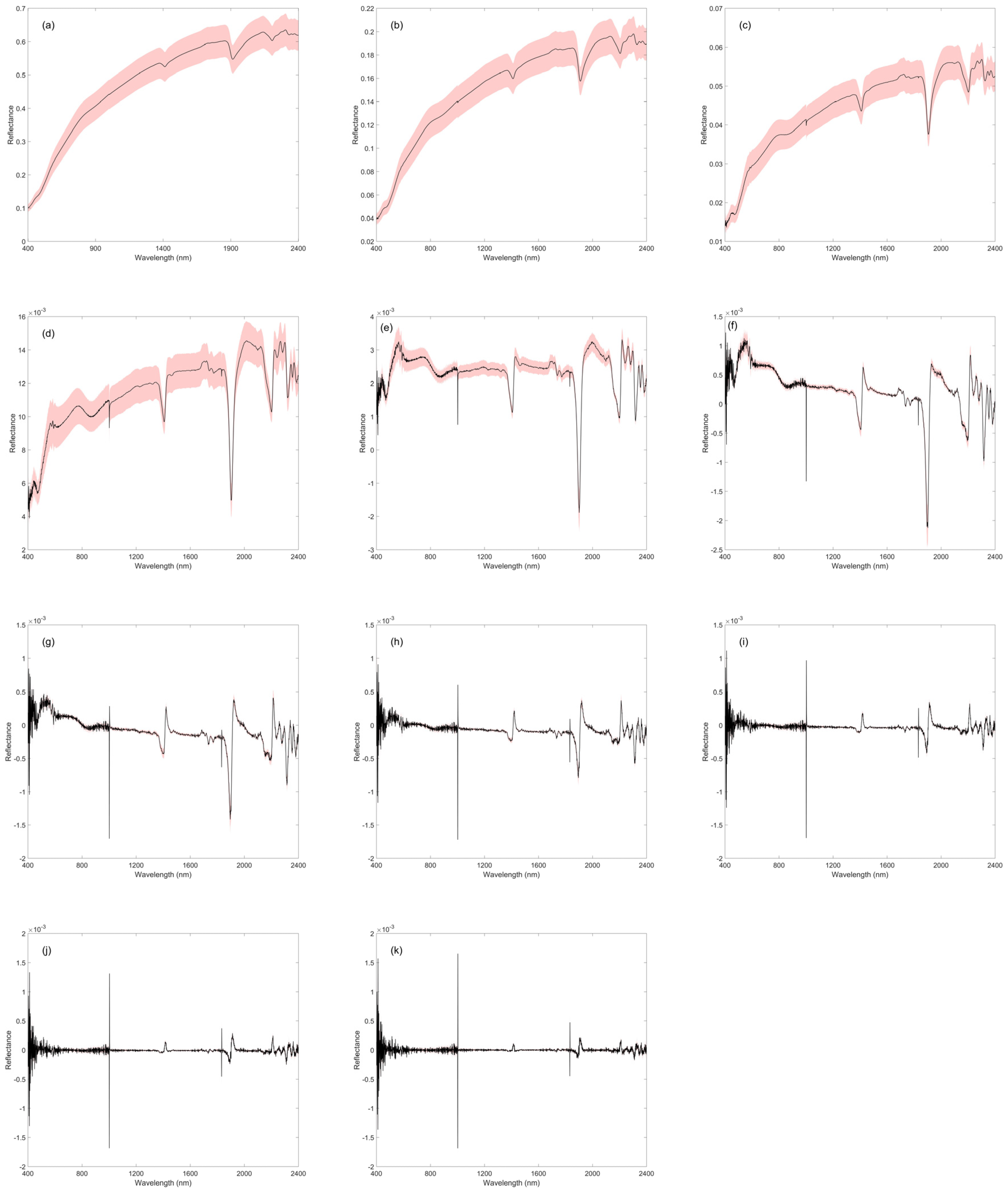
In the study of spectral derivatives, some researchers have reported that the first derivative produced higher model accuracy than the second derivative when estimating heavy metals and soil organic matter [72,73,74]. This phenomenon is related to the fact that the first derivative can enhance the spectral information while maintaining the continuity and integrity of spectral information, whereas the second derivative introduces additional spectral noise [20,72]. In 
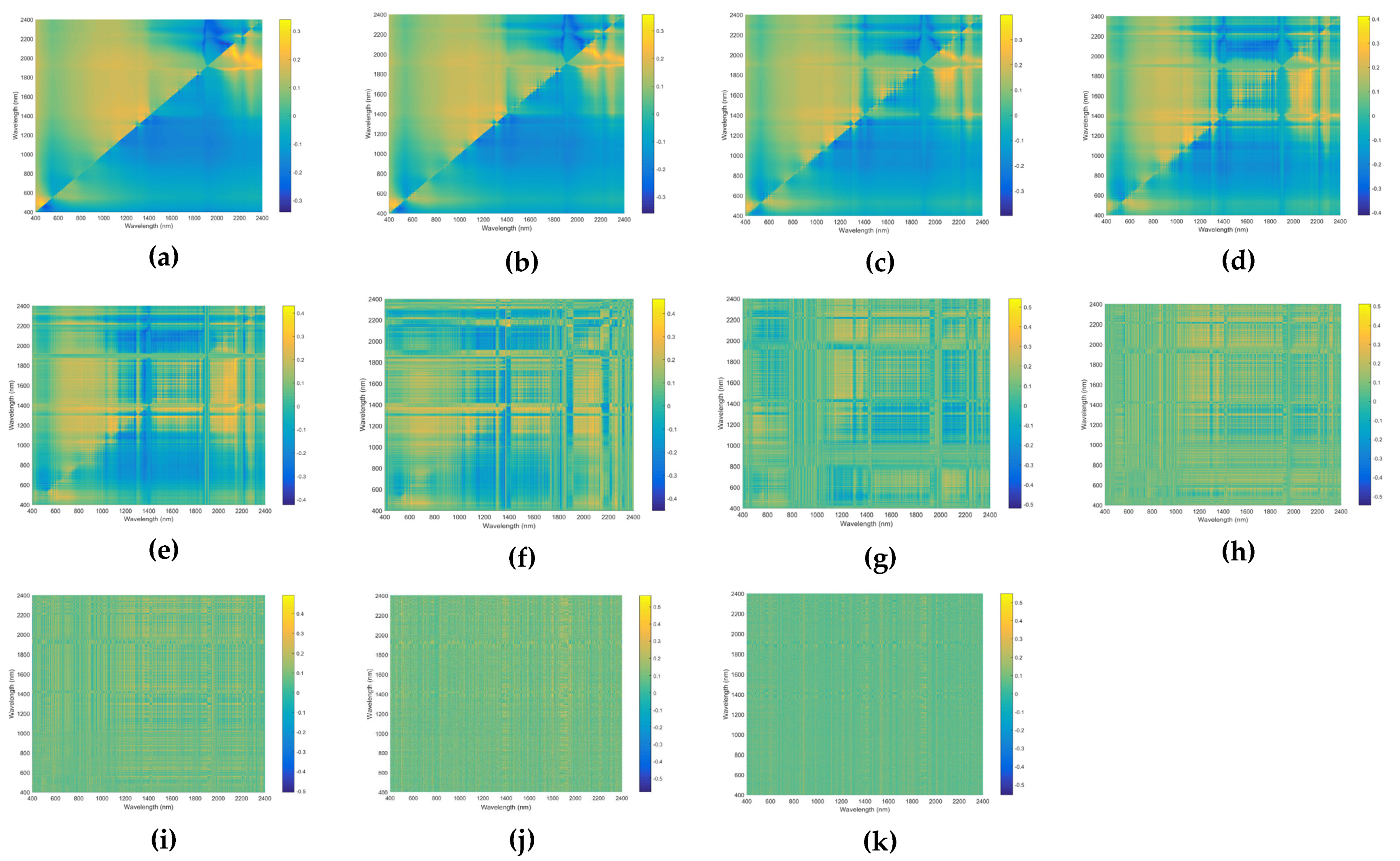
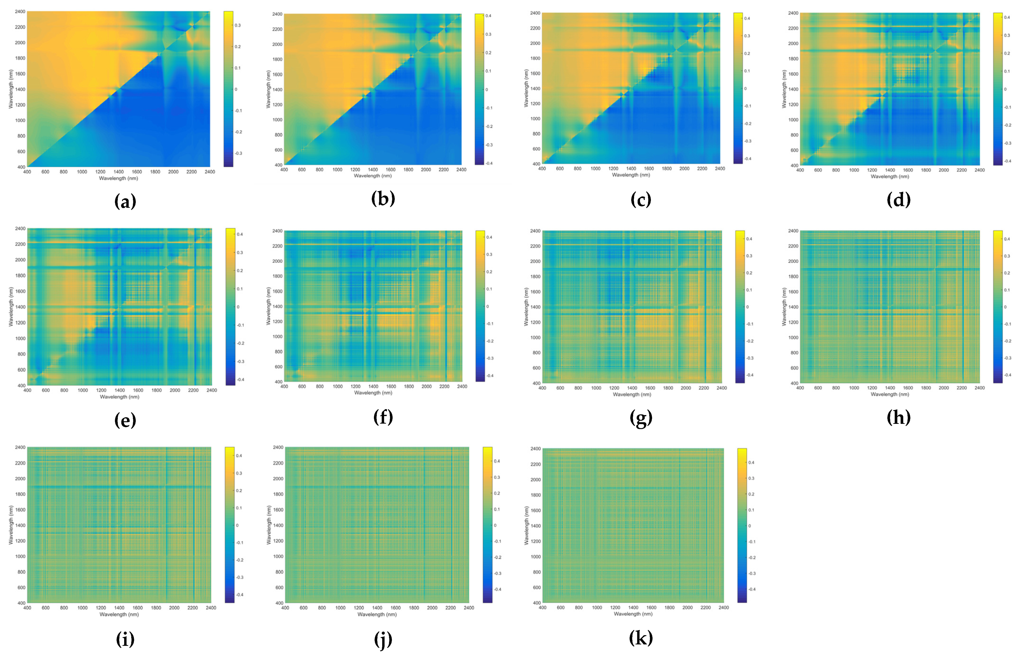
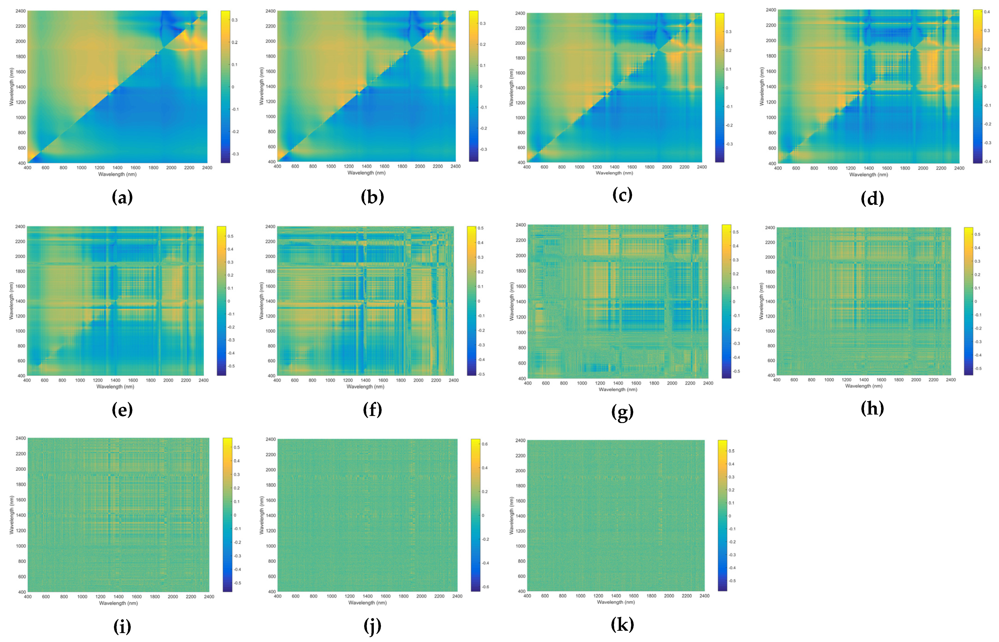
Figure 2, the second derivative spectrum fluctuated too frequently, indicating that the spectral information was disturbed by spectral noise. However, in this study, the accuracy of models using the first derivative was similar to those using the second derivative in the estimation of Cr and Cu, and the accuracy of models using the second derivative was higher than those using the first derivative in the estimation of Hg. How did this phenomenon happen in our experiment? After spectral derivatives, the spectra were processed by the optimal band combination algorithm. The algorithm selects the optimal bands, and carries on the mathematical transformation to the reflectance. In this process, the additional spectral noise caused by the high-order derivatives is removed. Furthermore, compared with low-order derivatives, high-order derivatives have the advantages of highlighting spectral information and separating the minor absorption peaks. Therefore, the accuracy of the models using the second derivative was similar to that of the first derivative, or even greatly improved. In addition to the removal of noise, the optimal band combination algorithm also has the ability to reduce the impact of irrelevant wavelength and cope with the overlapping absorption of soil components through considering wavelength interactions [48,75,76]. According to the spectral indices counted in Table 2, Table 3 and Table 4, a total of 19 wavelengths were selected from the spectra of three heavy metals, including 547 nm, 667 nm, 714 nm, 866 nm, 923 nm, 955 nm, 980 nm, 1011 nm, 1015 nm, 1129 nm, 1137 nm, 1173 nm, 1295 nm, 1562 nm, 1710 nm, 1969 nm, 2087 nm, 2342 nm, and 2346 nm. These wavelengths are close to the absorption characteristics of hematite, ferrihydrite, Fe3+, goethite, illite, organic matter, N-H, C-H, and O-H stretch [56,77]. The spectral characteristics of soil organic matter (SOM) and clay are closely related to the spectral response of N-H, C-H and O-H covalent bonds [78]. This is consistent with the absorption characteristics obtained. According to previous studies, due to the strong absorption capacity of SOM, iron oxides and clay, the Vis-NIR spectroscopy monitoring of heavy metals is through association with proxies (i.e., SOM, iron and clay) [79,80]. Therefore, Vis-NIR spectroscopy estimation for Hg, Cr and Cu can be performed indirectly through these components or functional groups.
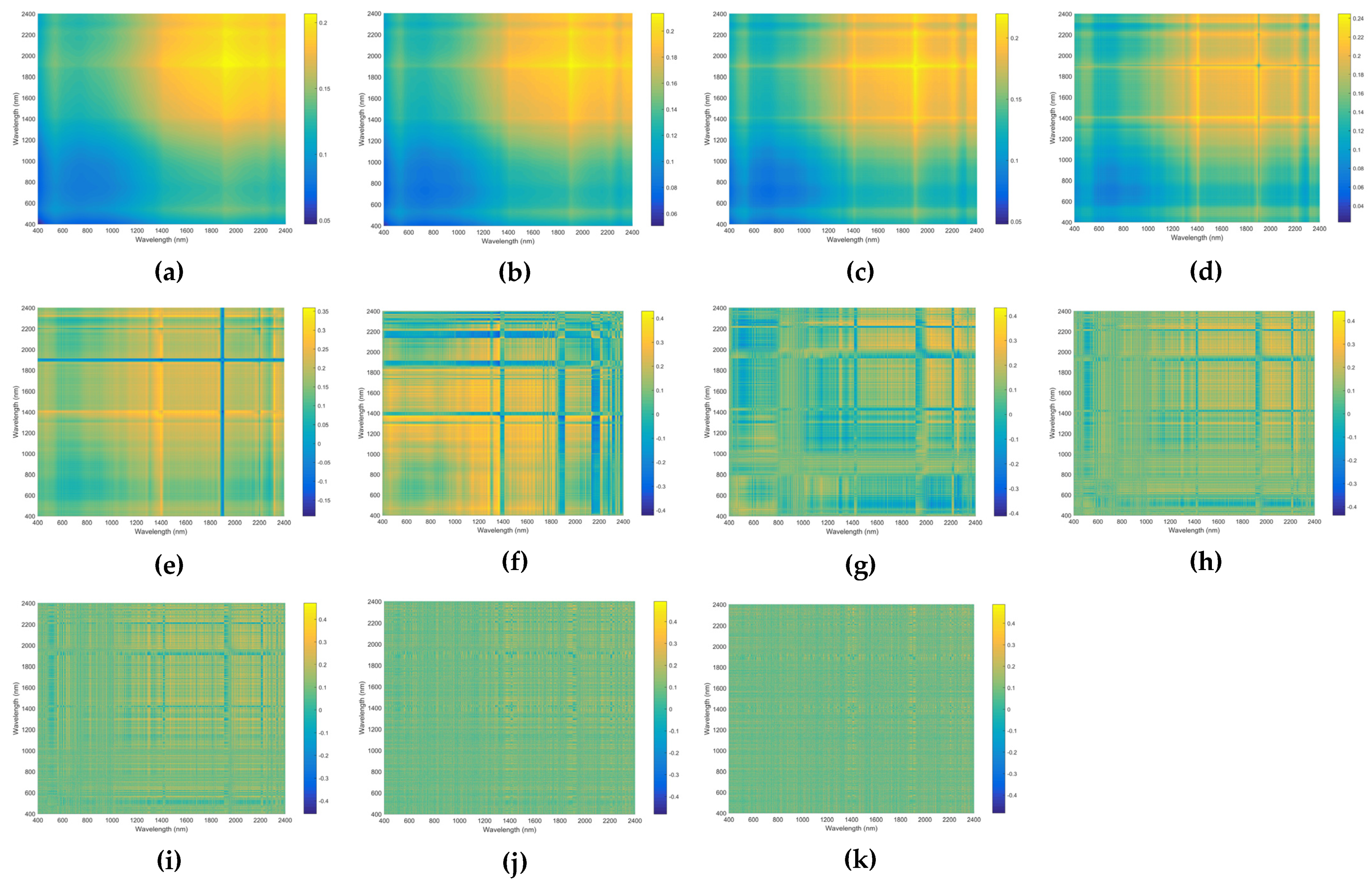
It is obvious that the spectra after the first derivative are quite different from those after the second derivative, and most of the subtle information changes are ignored. Table 2, Table 3 and Table 4 demonstrate how the correlation of spectral indices varies with the order of spectral derivatives. The characteristic bands of spectral indices have great variation in 1-order and 2-order. This showed that conventional spectral derivatives lost certain useful spectral information, and this loss of information is amplified by the optimal band combination algorithm. Additionally, the correlation coefficient of most spectral indices achieved the highest value between 1.2-order and 1.8-order, suggesting that FOD is able to detect more detailed spectral features compared with conventional spectral derivatives. 
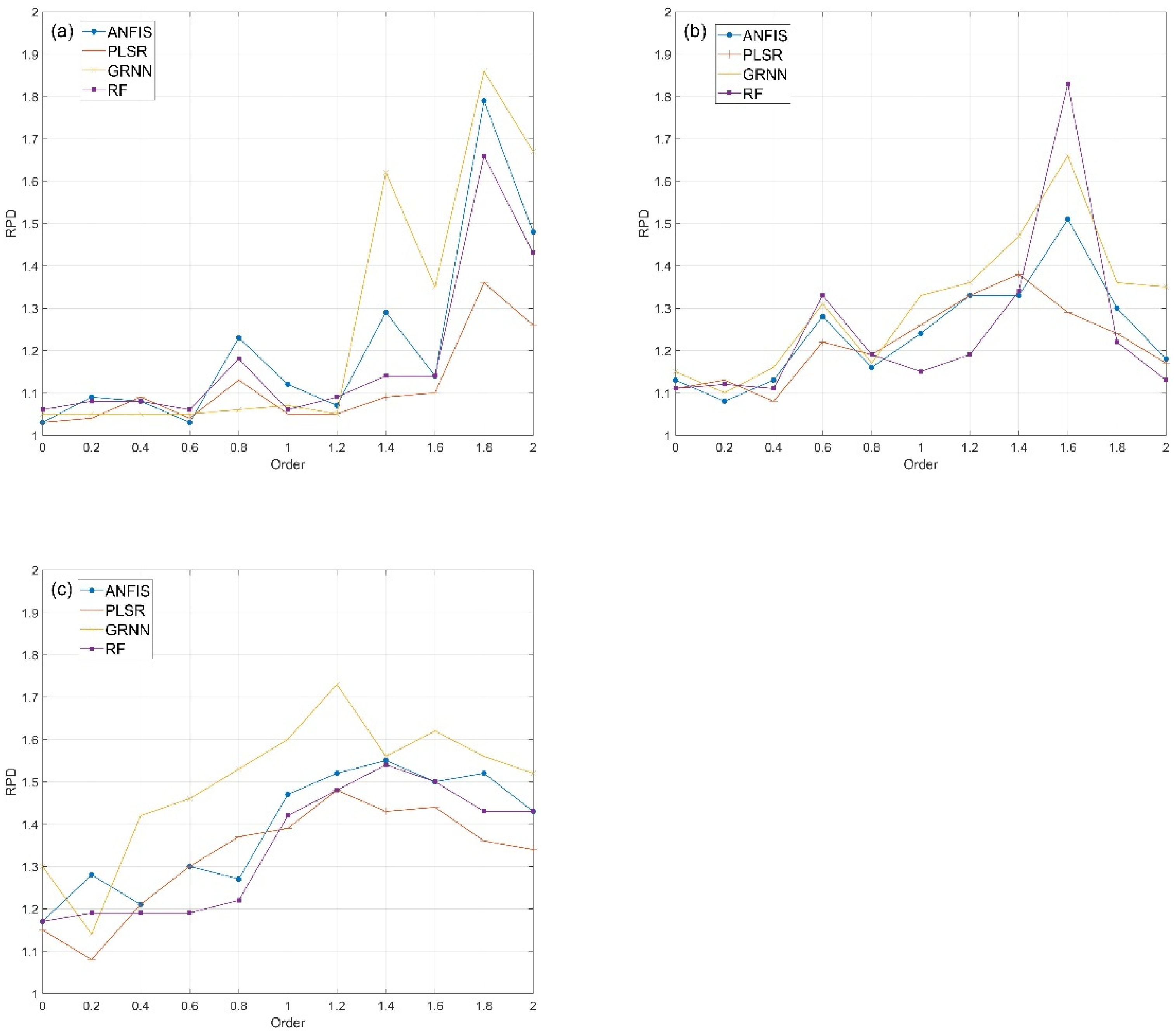
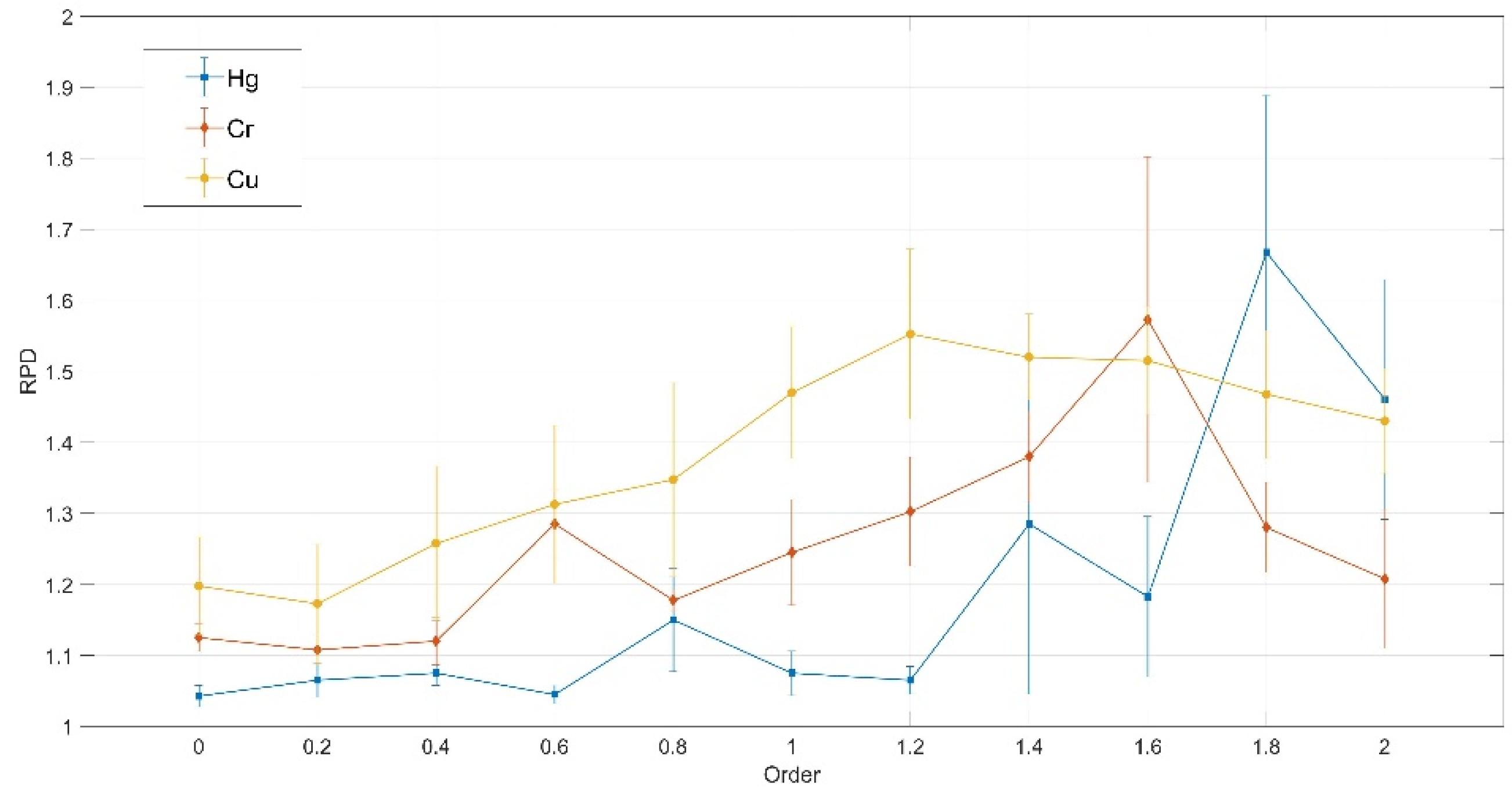
Figure 3 shows the variation in model accuracy after FOD and the four modeling methods. It can be seen that the models using FOD achieved better accuracy in the estimation of three heavy metals, regardless of the modeling method used, and the optimal models appeared at the 1.8-order, 1.6-order, and 1.2-order. Consistent with the optimal models, the maximum values of mean RPD for the models were also achieved at 1.8-order, 1.6-order and 1.2-order, which corresponded to Hg, Cr and Cu, respectively (Figure 4). This further indicates the advantages of high-order derivatives and the optimal band combination algorithm. High-order derivatives can highlight the hidden features in the spectrum, and the additional noise introduced by the high-order derivatives can be removed by the optimal band combination algorithm. The incorporation of the optimal band combination algorithm and FOD can enhance the estimation accuracy of heavy metals.
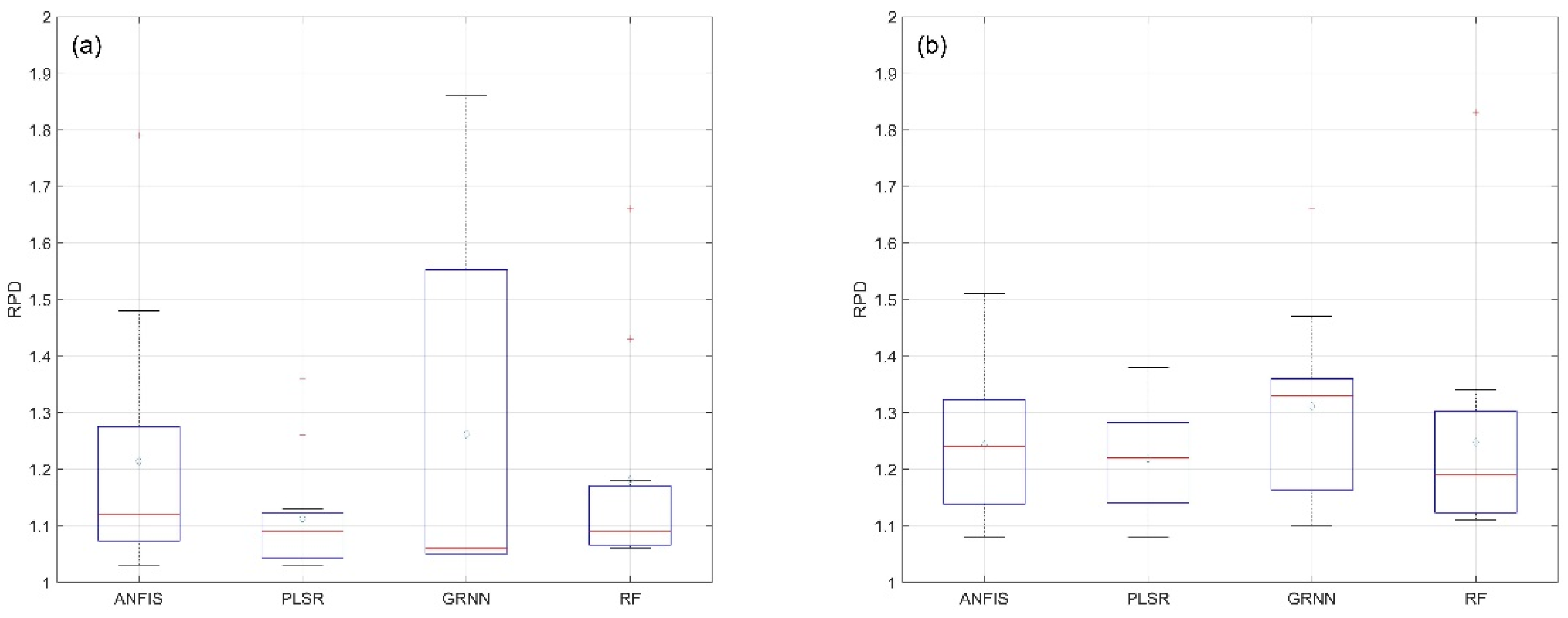
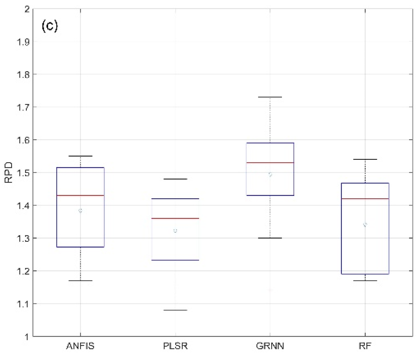
In the study, the ANFIS, PLSR, GRNN, and RF methods were applied to compare the estimation accuracy of the three heavy metal concentrations. According to Table 8, Table 9 and Table 10, the model accuracy listed in Table 5, Table 6 and Table 7 is influenced not only by FOD but also by modeling methods, and the more intuitive comparison of modeling methods is shown by boxplots (Figure 5). PLSR obtained the lowest mean value of model accuracy in the estimation of the three heavy metals. PLSR is only suitable for linear relationships [16,74,81]. However, there are various external or internal factors that can enhance the non-linear relationships between the Vis-NIR spectrum and soil components, such as measurement environment and characteristics of components [82,83]. Thus, compared with PLSR, the other three modeling methods are more suitable for estimation of heavy metals in soils due to their substantial non-linear prediction ability. Among ANFIS, RF and GRNN, GRNN showed the best performance in the estimation of heavy metal concentration. The GRNN has excellent capacity on non-linear mapping and learning speed; in particular, it has greater advantages in mapping unstable data to more accurate output [39,40,66]. Additionally, the range of target property is the fundamental factor of model accuracy [84]. The CV values reached 62.35%, 34.45%, and 28.58% for Hg, Cr, and Cu (Table 1), indicating heavy metal concentration in this study varied in a wide range with a high degree of dispersion. This is related to the outperformance of the models using GRNN.
In addition, the study also has some limitations. When dividing the dataset, more sample selection methods should be considered to enhance the stability of the experiment. For example, stratified sampling and Kennard–Stone sampling can be used to avoid taking the output property into account [85]. In the experiment, due to the high CV values of Hg, Cr and Cu in the samples, the models did not achieve high accuracy [84]. The representativeness of soil samples is significant for the estimation of heavy metals in soils using Vis-NIR spectroscopy. In future studies, this should be avoided by taking more soil samples. Furthermore, because of the optimal band combination algorithm, only five features were taken as input variables. This is related to the failure of RF to achieve better performance. Additionally, it is necessary to note the potential limitation of GRNN. It cannot ignore irrelevant inputs, thereby it is not likely to be suitable enough if existing more than five or six non-redundant inputs [66]. Thus, methods other than GRNN should be considered when using the full spectrum for modeling. The optimal results can be obtained by combining GRNN with appropriate dimensionality reduction methods, such as the optimal band combination algorithm.
The study of soil components is a multi-factor problem [86]. In the particular area, the lack of high-resolution spatial variability data always leads to substantial errors [87]. Using Vis-NIR spectroscopy can effectively reduce the workload of sampling, so as to obtain more spatial variability data. Thus, the incorporation of FOD, the optimal band combination algorithm and GRNN is a significant method for rapid evaluation of heavy metal concentration in agricultural soils.

5. Conclusions

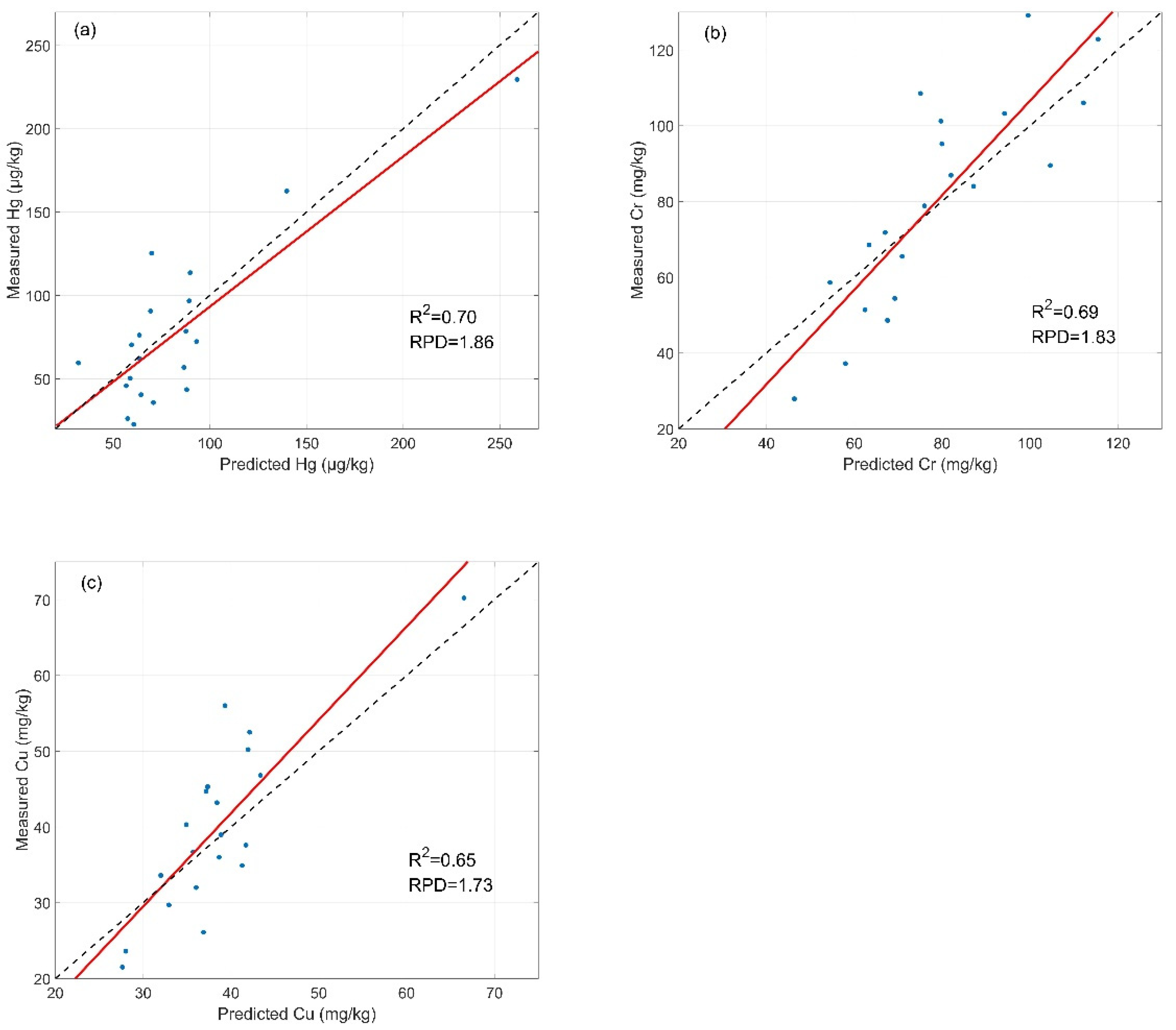
In this study, the potential of Vis-NIR spectroscopy to estimate the concentration of Hg, Cr, and Cu in soils was evaluated. Through the incorporation of FOD, the optimal band combination algorithm and modeling methods, the optimal models of Hg, Cr, and Cu were obtained. The optimal validation accuracy of Hg (R2 = 0.70, RPD = 1.86) and Cu (R2 = 0.65, RPD = 1.73) was achieved by the 1.8-order and 1.2-order reflectance GRNN model, and the optimal estimated accuracy of Cr (R2 = 0.69, RPD = 1.83) was achieved by the 1.6-order reflectance RF model. The optimal band combination algorithm is able to avoid the influence of spectral noise caused by high-order derivatives. Compared with conventional derivatives, FOD can identify the subtler spectral characteristics of heavy metals due to its gradual change in treatment of the spectrum. The high-order FOD is able to highlight hidden information and the separate minor absorbing peak. In addition, the incorporation of the optimal band combination algorithm and high-order FOD can further mine spectral information, ignoring noise. The optimal performance was achieved by the 1.8-order, 1.6-order, and 1.2-order spectra for Hg, Cr, and Cu, correspondingly. For estimation of heavy metals in soils, the modeling methods with the ability to solve non-linear problems are more suitable. When using the appropriate dimensionality reduction method, GRNN provides an obvious improvement to the estimation accuracy of all studied heavy metals compared to ANFIS, PLSR, and RF. Thus, the incorporation of the optimal band combination algorithm, FOD, and GRNN for the rapid spectral estimation of Hg, Cr, and Cu concentration was proven to be feasible. Additionally, this study is vital for the application of Vis-NIR spectroscopy technology to the investigation of other heavy metal contaminants in soils. In the future, we will conduct more studies to detect the influence of GRNN and FOD on Vis-NIR spectroscopy estimation of soil heavy metals through large soil spectral libraries.

Author Contributions

All of the authors contributed to the study. X.X. conceived and designed the experiments, analyzed the data and wrote the manuscript. X.X. and Y.Z. processed the data. L.R., C.H., D.L. and F.A. contributed greatly to data collection. S.C. reviewed the manuscript. All authors have read and agreed to the published version of the manuscript.

Funding

This research was funded by the National Key Research and Development Program of China (Grant No. 2020YFA0714103) and the program for JLU science and technology innovative research team (Grant No. JLUSTIRT, 2017TD-26).

Acknowledgments

We thank the editors and reviewers for their constructive suggestions and insightful comments, which helped us greatly improve this manuscript. Furthermore, we also appreciate the help of publisher in the process.

Conflicts of Interest

The authors declare no conflict of interest.

Appendix A

The correlations coefficients between Hg and the RI, DI, NDI, PI and SI indices of the spectra after FOD are shown in Figure A1, Figure A2, Figure A3, Figure A4 and Figure A5, respectively.
Figure A1. Correlation coefficients between soil Hg and ratio index of the reflectance processed by (a) 0-order, (b) 0.2-order, (c) 0.4-order, (d) 0.6-order, (e) 0.8-order, (f) 1-order, (g) 1.2-order, (h) 1.4-order, (i) 1.6-order, (j) 1.8-order, (k) 2-order.
Remotesensing 13 02718 g0a1
Figure A2. Correlation coefficients between soil Hg and difference index of the reflectance processed by (a) 0-order, (b) 0.2-order, (c) 0.4-order, (d) 0.6-order, (e) 0.8-order, (f) 1-order, (g) 1.2-order, (h) 1.4-order, (i) 1.6-order, (j) 1.8-order, (k) 2-order.
Remotesensing 13 02718 g0a2
Figure A3. Correlation coefficients between soil Hg and normalized difference index of the reflectance processed by (a) 0-order, (b) 0.2-order, (c) 0.4-order, (d) 0.6-order, (e) 0.8-order, (f) 1-order, (g) 1.2-order, (h) 1.4-order, (i) 1.6-order, (j) 1.8-order, (k) 2-order.
Remotesensing 13 02718 g0a3
Figure A4. Correlation coefficients between soil Hg and product index of the reflectance processed by (a) 0-order, (b) 0.2-order, (c) 0.4-order, (d) 0.6-order, (e) 0.8-order, (f) 1-order, (g) 1.2-order, (h) 1.4-order, (i) 1.6-order, (j) 1.8-order, (k) 2-order.
Remotesensing 13 02718 g0a4
Figure A5. Correlation coefficients between soil Hg and sum index of the reflectance processed by (a) 0-order, (b) 0.2-order, (c) 0.4-order, (d) 0.6-order, (e) 0.8-order, (f) 1-order, (g) 1.2-order, (h) 1.4-order, (i) 1.6-order, (j) 1.8-order, (k) 2-order.
Remotesensing 13 02718 g0a5

References

  1. Horta, A.; Malone, B.; Stockmann, U.; Minasny, B.; Bishop, T.; McBratney, A.; Pallasser, R.; Pozza, L. Potential of integrated field spectroscopy and spatial analysis for enhanced assessment of soil contamination: A prospective review. Geoderma 2015, 241, 180–209. [Google Scholar] [CrossRef] [Green Version]
  2. Seleiman, M.F.; Santanen, A.; Mäkelä, P.S. Recycling sludge on cropland as fertilizer–Advantages and risks. Resour. Conserv. Recycl. 2020, 155, 104647. [Google Scholar] [CrossRef]
  3. Xu, D.; Chen, S.; Xu, H.; Wang, N.; Zhou, Y.; Shi, Z. Data fusion for the measurement of potentially toxic elements in soil using portable spectrometers. Environ. Pollut. 2020, 263, 114649. [Google Scholar] [CrossRef]
  4. Dong, W.Q.Y.; Cui, Y.; Liu, X. Instances of soil and crop heavy metal contamination in China. Soil Sediment Contam. 2001, 10, 497–510. [Google Scholar] [CrossRef]
  5. Dong, J.; Yang, Q.-w.; Sun, L.-n.; Zeng, Q.; Liu, S.-j.; Pan, J.; Liu, X.-l. Assessing the concentration and potential dietary risk of heavy metals in vegetables at a Pb/Zn mine site, China. Environ. Earth Sci. 2011, 64, 1317–1321. [Google Scholar] [CrossRef]
  6. Jia, X.; Hu, B.; Marchant, B.P.; Zhou, L.; Shi, Z.; Zhu, Y. A methodological framework for identifying potential sources of soil heavy metal pollution based on machine learning: A case study in the Yangtze Delta, China. Environ. Pollut. 2019, 250, 601–609. [Google Scholar] [CrossRef] [PubMed]
  7. Clarke, B.O.; Smith, S.R. Review of ‘emerging’organic contaminants in biosolids and assessment of international research priorities for the agricultural use of biosolids. Environ. Int. 2011, 37, 226–247. [Google Scholar] [CrossRef] [PubMed]
  8. Ali, S.; Abbas, Z.; Seleiman, M.F.; Rizwan, M.; YavaŞ, İ.; Alhammad, B.A.; Shami, A.; Hasanuzzaman, M.; Kalderis, D. Glycine Betaine Accumulation, Significance and Interests for Heavy Metal Tolerance in Plants. Plants 2020, 9, 896. [Google Scholar] [CrossRef]
  9. Fang, F.; Wang, H.; Lin, Y. Spatial distribution, bioavailability, and health risk assessment of soil Hg in Wuhu urban area, China. Environ. Monit. 2011, 179, 255–265. [Google Scholar] [CrossRef]
  10. De Temmerman, L.; Waegeneers, N.; Claeys, N.; Roekens, E. Comparison of concentrations of mercury in ambient air to its accumulation by leafy vegetables: An important step in terrestrial food chain analysis. Environ. Pollut. 2009, 157, 1337–1341. [Google Scholar] [CrossRef]
  11. Wu, J.; Zhang, J.; Xiao, C. Focus on factors affecting pH, flow of Cr and transformation between Cr (VI) and Cr (III) in the soil with different electrolytes. Electrochim. Acta 2016, 211, 652–662. [Google Scholar] [CrossRef]
  12. Andrade, S.A.; Gratão, P.L.; Azevedo, R.A.; Silveira, A.P.; Schiavinato, M.A.; Mazzafera, P. Biochemical and physiological changes in jack bean under mycorrhizal symbiosis growing in soil with increasing Cu concentrations. Environ. Exp. Bot. 2010, 68, 198–207. [Google Scholar] [CrossRef]
  13. Chakraborty, S.; Man, T.; Paulette, L.; Deb, S.; Li, B.; Weindorf, D.; Frazier, M. Rapid assessment of smelter/mining soil contamination via portable X-ray fluorescence spectrometry and indicator kriging. Geoderma 2017, 306, 108–119. [Google Scholar] [CrossRef]
  14. Shi, T.; Yang, C.; Liu, H.; Wu, C.; Wang, Z.; Li, H.; Zhang, H.; Guo, L.; Wu, G.; Su, F. Mapping lead concentrations in urban topsoil using proximal and remote sensing data and hybrid statistical approaches. Environ. Pollut. 2021, 272, 116041. [Google Scholar] [CrossRef]
  15. Morellos, A.; Pantazi, X.-E.; Moshou, D.; Alexandridis, T.; Whetton, R.; Tziotzios, G.; Wiebensohn, J.; Bill, R.; Mouazen, A.M. Machine learning based prediction of soil total nitrogen, organic carbon and moisture content by using VIS-NIR spectroscopy. Biosyst. Eng. 2016, 152, 104–116. [Google Scholar] [CrossRef] [Green Version]
  16. Xu, S.; Zhao, Y.; Wang, M.; Shi, X. Comparison of multivariate methods for estimating selected soil properties from intact soil cores of paddy fields by Vis–NIR spectroscopy. Geoderma 2018, 310, 29–43. [Google Scholar] [CrossRef]
  17. Liu, J.; Zhang, Y.; Wang, H.; Du, Y. Study on the prediction of soil heavy metal elements content based on visible near-infrared spectroscopy. Spectrochim. Acta Part A Mol. Biomol. Spectrosc. 2018, 199, 43–49. [Google Scholar] [CrossRef]
  18. Stenberg, B.; Rossel, R.A.V.; Mouazen, A.M.; Wetterlind, J. Visible and near infrared spectroscopy in soil science. Adv. Agron. 2010, 107, 163–215. [Google Scholar]
  19. Tekin, Y.; Kuang, B.; Mouazen, A.M. Potential of on-line visible and near infrared spectroscopy for measurement of pH for deriving variable rate lime recommendations. Sensors 2013, 13, 10177–10190. [Google Scholar] [CrossRef] [PubMed]
  20. Khosravi, V.; Ardejani, F.D.; Yousefi, S.; Aryafar, A. Monitoring soil lead and zinc contents via combination of spectroscopy with extreme learning machine and other data mining methods. Geoderma 2018, 318, 29–41. [Google Scholar] [CrossRef]
  21. Xu, X.; Chen, S.; Xu, Z.; Yu, Y.; Zhang, S.; Dai, R. Exploring Appropriate Preprocessing Techniques for Hyperspectral Soil Organic Matter Content Estimation in Black Soil Area. Remote Sens. 2020, 12, 3765. [Google Scholar] [CrossRef]
  22. Douglas, R.K.; Nawar, S.; Cipullo, S.; Alamar, M.C.; Coulon, F.; Mouazen, A. Evaluation of vis-NIR reflectance spectroscopy sensitivity to weathering for enhanced assessment of oil contaminated soils. Sci. Total Environ. 2018, 626, 1108–1120. [Google Scholar] [CrossRef] [Green Version]
  23. Hong, Y.; Shen, R.; Cheng, H.; Chen, S.; Chen, Y.; Guo, L.; He, J.; Liu, Y.; Yu, L.; Liu, Y. Cadmium concentration estimation in peri-urban agricultural soils: Using reflectance spectroscopy, soil auxiliary information, or a combination of both? Geoderma 2019, 354, 113875. [Google Scholar] [CrossRef]
  24. Guo, P.-T.; Li, M.-F.; Luo, W.; Tang, Q.-F.; Liu, Z.-W.; Lin, Z.-M. Digital mapping of soil organic matter for rubber plantation at regional scale: An application of random forest plus residuals kriging approach. Geoderma 2015, 237, 49–59. [Google Scholar] [CrossRef]
  25. Wang, F.; Gao, J.; Zha, Y. Hyperspectral sensing of heavy metals in soil and vegetation: Feasibility and challenges. ISPRS J. Photogramm. Remote Sens. 2018, 136, 73–84. [Google Scholar] [CrossRef]
  26. Chen, L.; Tan, K. Estimation of Soil Heavy Metal Combining Fractional Order Derivative. Int. Arch. Photogramm. Remote Sens. Spat. Inf. Sci. 2020, 43, 1439–1444. [Google Scholar] [CrossRef]
  27. Hong, Y.; Shen, R.; Cheng, H.; Chen, Y.; Zhang, Y.; Liu, Y.; Zhou, M.; Yu, L.; Liu, Y.; Liu, Y. Estimating lead and zinc concentrations in peri-urban agricultural soils through reflectance spectroscopy: Effects of fractional-order derivative and random forest. Sci. Total Environ. 2019, 651, 1969–1982. [Google Scholar] [CrossRef]
  28. Vašát, R.; Kodešová, R.; Borůvka, L.; Jakšík, O.; Klement, A.; Brodský, L. Combining reflectance spectroscopy and the digital elevation model for soil oxidizable carbon estimation. Geoderma 2017, 303, 133–142. [Google Scholar] [CrossRef]
  29. Jin, X.; Du, J.; Liu, H.; Wang, Z.; Song, K. Remote estimation of soil organic matter content in the Sanjiang Plain, Northest China: The optimal band algorithm versus the GRA-ANN model. Agric. For. Meteorol. 2016, 218, 250–260. [Google Scholar] [CrossRef]
  30. Gholizadeh, A.; Borůvka, L.; Saberioon, M.; Vašát, R. A memory-based learning approach as compared to other data mining algorithms for the prediction of soil texture using diffuse reflectance spectra. Remote Sens. 2016, 8, 341. [Google Scholar] [CrossRef] [Green Version]
  31. Dong, J.; Dai, W.; Xu, J.; Li, S. Spectral estimation model construction of heavy metals in mining reclamation areas. Int. J. Environ. Res. Public Health 2016, 13, 640. [Google Scholar] [CrossRef] [Green Version]
  32. Wang, J.; Cui, L.; Gao, W.; Shi, T.; Chen, Y.; Gao, Y. Prediction of low heavy metal concentrations in agricultural soils using visible and near-infrared reflectance spectroscopy. Geoderma 2014, 216, 1–9. [Google Scholar] [CrossRef]
  33. Tan, K.; Ye, Y.-Y.; Du, P.-J.; Zhang, Q.-Q. Estimation of heavy metal concentrations in reclaimed mining soils using reflectance spectroscopy. Spectrosc. Spectr. Anal. 2014, 34, 3317–3322. [Google Scholar]
  34. Tan, K.; Ye, Y.; Cao, Q.; Du, P.; Dong, J. Estimation of arsenic contamination in reclaimed agricultural soils using reflectance spectroscopy and ANFIS model. IEEE J. Sel. Top. Appl. Earth Obs. Remote Sens. 2014, 7, 2540–2546. [Google Scholar] [CrossRef]
  35. Tan, K.; Ma, W.; Wu, F.; Du, Q. Random forest–based estimation of heavy metal concentration in agricultural soils with hyperspectral sensor data. Environ. Monit. Assess. 2019, 191, 1–14. [Google Scholar] [CrossRef]
  36. Luo, W.; Fu, Z. Application of generalized regression neural network to the agricultural machinery demand forecasting. Appl. Mech. Mater. 2013, 278-280, 2177–2181. [Google Scholar] [CrossRef]
  37. Feng, Y.; Cui, N.; Gong, D.; Zhang, Q.; Zhao, L. Evaluation of random forests and generalized regression neural networks for daily reference evapotranspiration modelling. Agric. Water Manag. 2017, 193, 163–173. [Google Scholar] [CrossRef]
  38. Wang, L.; Kisi, O.; Zounemat-Kermani, M.; Li, H. Pan evaporation modeling using six different heuristic computing methods in different climates of China. J. Hydrol. 2017, 544, 407–427. [Google Scholar] [CrossRef]
  39. Zhang, Y.; Zhao, Z.; Zheng, J. CatBoost: A new approach for estimating daily reference crop evapotranspiration in arid and semi-arid regions of Northern China. J. Hydrol. 2020, 588, 125087. [Google Scholar] [CrossRef]
  40. Yan, H.; Mou, Y.; Xu, X.; Du, J.; Wang, R.; Liu, P. A comparative assessment of predicting CH4 adsorption on different activated carbons using generalized regression neural network (GRNN), and adaptive network-based fuzzy inference system (ANFIS). Energy Sources Part A Recovery Util. Environ. Eff. 2019, 41, 1983–1992. [Google Scholar] [CrossRef]
  41. Micheli, E.; Schad, P.; Spaargaren, O.; Dent, D. World Reference Base for Soil Resources 2006: A Framework for International Classification, Correlation and Communication; Food and Agriculture Organization of the United Nations (FAO): Rome, Italy, 2006. [Google Scholar]
  42. Savitzky, A.; Golay, M.J. Smoothing and differentiation of data by simplified least squares procedures. Anal. Chem. 1964, 36, 1627–1639. [Google Scholar] [CrossRef]
  43. Wang, B.; Waters, C.; Orgill, S.; Cowie, A.; Clark, A.; Li Liu, D.; Simpson, M.; McGowen, I.; Sides, T. Estimating soil organic carbon stocks using different modelling techniques in the semi-arid rangelands of eastern Australia. Ecol. Indic. 2018, 88, 425–438. [Google Scholar] [CrossRef]
  44. Hong, Y.; Liu, Y.; Chen, Y.; Liu, Y.; Yu, L.; Liu, Y.; Cheng, H. Application of fractional-order derivative in the quantitative estimation of soil organic matter content through visible and near-infrared spectroscopy. Geoderma 2019, 337, 758–769. [Google Scholar] [CrossRef]
  45. Inoue, Y.; Peñuelas, J.; Miyata, A.; Mano, M. Normalized difference spectral indices for estimating photosynthetic efficiency and capacity at a canopy scale derived from hyperspectral and CO2 flux measurements in rice. Remote Sens. Environ. 2008, 112, 156–172. [Google Scholar] [CrossRef]
  46. Tian, Y.; Zhang, J.; Yao, X.; Cao, W.; Zhu, Y. Laboratory assessment of three quantitative methods for estimating the organic matter content of soils in China based on visible/near-infrared reflectance spectra. Geoderma 2013, 202, 161–170. [Google Scholar] [CrossRef]
  47. Wang, X.; Zhang, F.; Johnson, V.C. New methods for improving the remote sensing estimation of soil organic matter content (SOMC) in the Ebinur Lake Wetland National Nature Reserve (ELWNNR) in northwest China. Remote Sens. Environ. 2018, 218, 104–118. [Google Scholar] [CrossRef]
  48. Nawar, S.; Buddenbaum, H.; Hill, J. Estimation of soil salinity using three quantitative methods based on visible and near-infrared reflectance spectroscopy: A case study from Egypt. Arab. J. Geosci. 2015, 8, 5127–5140. [Google Scholar] [CrossRef]
  49. Inoue, Y.; Sakaiya, E.; Zhu, Y.; Takahashi, W. Diagnostic mapping of canopy nitrogen content in rice based on hyperspectral measurements. Remote Sens. Environ. 2012, 126, 210–221. [Google Scholar] [CrossRef]
  50. Wang, X.; Zhang, F.; Ding, J.; Latif, A.; Johnson, V.C. Estimation of soil salt content (SSC) in the Ebinur Lake Wetland National Nature Reserve (ELWNNR), Northwest China, based on a Bootstrap-BP neural network model and optimal spectral indices. Sci. Total Environ. 2018, 615, 918–930. [Google Scholar] [CrossRef]
  51. Podlubny, I. Fractional Differential Equations: An Introduction to Fractional Derivatives, Fractional Differential Equations, to Methods of Their Solution and Some of Their Applications; Elsevier: Amsterdam, The Netherlands, 1998. [Google Scholar]
  52. Sierociuk, D.; Skovranek, T.; Macias, M.; Podlubny, I.; Petras, I.; Dzielinski, A.; Ziubinski, P. Diffusion process modeling by using fractional-order models. Appl. Math. Comput. 2015, 257, 2–11. [Google Scholar] [CrossRef] [Green Version]
  53. Geladi, P.; Kowalski, B.R. Partial least-squares regression: A tutorial. Anal. Chim. Acta 1986, 185, 1–17. [Google Scholar] [CrossRef]
  54. Yi, Q.; Jiapaer, G.; Chen, J.; Bao, A.; Wang, F. Different units of measurement of carotenoids estimation in cotton using hyperspectral indices and partial least square regression. ISPRS J. Photogramm. Remote Sens. 2014, 91, 72–84. [Google Scholar] [CrossRef]
  55. Dotto, A.C.; Dalmolin, R.S.D.; ten Caten, A.; Grunwald, S. A systematic study on the application of scatter-corrective and spectral-derivative preprocessing for multivariate prediction of soil organic carbon by Vis-NIR spectra. Geoderma 2018, 314, 262–274. [Google Scholar] [CrossRef]
  56. Rossel, R.V.; Behrens, T. Using data mining to model and interpret soil diffuse reflectance spectra. Geoderma 2010, 158, 46–54. [Google Scholar] [CrossRef]
  57. Breiman, L. Random forests. Mach. Learn. 2001, 45, 5–32. [Google Scholar] [CrossRef] [Green Version]
  58. Chen, S.; Martin, M.P.; Saby, N.P.; Walter, C.; Angers, D.A.; Arrouays, D. Fine resolution map of top-and subsoil carbon sequestration potential in France. Sci. Total Environ. 2018, 630, 389–400. [Google Scholar] [CrossRef]
  59. Peters, J.; De Baets, B.; Verhoest, N.E.; Samson, R.; Degroeve, S.; De Becker, P.; Huybrechts, W. Random forests as a tool for ecohydrological distribution modelling. Ecol. Model. 2007, 207, 304–318. [Google Scholar] [CrossRef]
  60. Keskin, H.; Grunwald, S.; Harris, W.G. Digital mapping of soil carbon fractions with machine learning. Geoderma 2019, 339, 40–58. [Google Scholar] [CrossRef]
  61. Liaw, A.; Wiener, M. Classification and regression by random Forest. R News 2002, 2, 18–22. [Google Scholar]
  62. Loukas, Y.L. Adaptive neuro-fuzzy inference system: An instant and architecture-free predictor for improved QSAR studies. J. Med. Chem. 2001, 44, 2772–2783. [Google Scholar] [CrossRef]
  63. Rahmanian, B.; Pakizeh, M.; Mansoori, S.A.A.; Esfandyari, M.; Jafari, D.; Maddah, H.; Maskooki, A. Prediction of MEUF process performance using artificial neural networks and ANFIS approaches. J. Taiwan Inst. Chem. Eng. 2012, 43, 558–565. [Google Scholar] [CrossRef]
  64. Specht, D.F. A general regression neural network. IEEE Trans. Neural Netw. 1991, 2, 568–576. [Google Scholar] [CrossRef] [Green Version]
  65. Kamel, A.H.; Afan, H.A.; Sherif, M.; Ahmed, A.N.; El-Shafie, A. RBFNN versus GRNN modeling approach for sub-surface evaporation rate prediction in arid region. Sustain. Comput. Inform. Syst. 2021, 30, 100514. [Google Scholar]
  66. Rooki, R.; Ardejani, F.D.; Aryafar, A.; Asadi, A.B. Prediction of heavy metals in acid mine drainage using artificial neural network from the Shur River of the Sarcheshmeh porphyry copper mine, Southeast Iran. Environ. Earth Sci. 2011, 64, 1303–1316. [Google Scholar] [CrossRef]
  67. CNMEE. Soil Environmental Quality Risk Control Standard for Soil Contamination of Agricultural Land; Ministry of Ecology and Environment of China: Beijing, China, 2018.
  68. China Environmental Monitoring Station. Chinese Soil Element Background Value; China Environmental Science Press: Beijing, China, 1990. [Google Scholar]
  69. Chen, T.; Chang, Q.; Liu, J.; Clevers, J.; Kooistra, L. Identification of soil heavy metal sources and improvement in spatial mapping based on soil spectral information: A case study in northwest China. Sci. Total Environ. 2016, 565, 155–164. [Google Scholar] [CrossRef]
  70. D’amore, J.; Al-Abed, S.; Scheckel, K.; Ryan, J. Methods for speciation of metals in soils: A review. J. Environ. Qual. 2005, 34, 1707–1745. [Google Scholar] [CrossRef] [PubMed] [Green Version]
  71. Hu, W.; Huang, B.; Shi, X.; Chen, W.; Zhao, Y.; Jiao, W. Accumulation and health risk of heavy metals in a plot-scale vegetable production system in a peri-urban vegetable farm near Nanjing, China. Ecotoxicol. Environ. Saf. 2013, 98, 303–309. [Google Scholar] [CrossRef] [PubMed]
  72. Chakraborty, S.; Weindorf, D.C.; Deb, S.; Li, B.; Paul, S.; Choudhury, A.; Ray, D.P. Rapid assessment of regional soil arsenic pollution risk via diffuse reflectance spectroscopy. Geoderma 2017, 289, 72–81. [Google Scholar] [CrossRef]
  73. Gao, Y.; Cui, L.; Lei, B.; Zhai, Y.; Shi, T.; Wang, J.; Chen, Y.; He, H.; Wu, G. Estimating soil organic carbon content with visible-near-infrared (Vis-NIR) spectroscopy. Appl. Spectrosc. 2014, 68, 712–722. [Google Scholar] [CrossRef] [PubMed]
  74. Nawar, S.; Buddenbaum, H.; Hill, J.; Kozak, J.; Mouazen, A.M. Estimating the soil clay content and organic matter by means of different calibration methods of vis-NIR diffuse reflectance spectroscopy. Soil Tillage Res. 2016, 155, 510–522. [Google Scholar] [CrossRef] [Green Version]
  75. Bao, N.; Wu, L.; Ye, B.; Yang, K.; Zhou, W. Assessing soil organic matter of reclaimed soil from a large surface coal mine using a field spectroradiometer in laboratory. Geoderma 2017, 288, 47–55. [Google Scholar] [CrossRef]
  76. Shi, T.; Liu, H.; Chen, Y.; Wang, J.; Wu, G. Estimation of arsenic in agricultural soils using hyperspectral vegetation indices of rice. J. Hazard. Mater. 2016, 308, 243–252. [Google Scholar] [CrossRef]
  77. Knadel, M.; Viscarra Rossel, R.A.; Deng, F.; Thomsen, A.; Greve, M.H. Visible–near infrared spectra as a proxy for topsoil texture and glacial boundaries. Soil Sci. Soc. Am. J. 2013, 77, 568–579. [Google Scholar] [CrossRef]
  78. Rossel, R.V.; Walvoort, D.; McBratney, A.; Janik, L.J.; Skjemstad, J. Visible, near infrared, mid infrared or combined diffuse reflectance spectroscopy for simultaneous assessment of various soil properties. Geoderma 2006, 131, 59–75. [Google Scholar] [CrossRef]
  79. Zhang, X.; Sun, W.; Cen, Y.; Zhang, L.; Wang, N. Predicting cadmium concentration in soils using laboratory and field reflectance spectroscopy. Sci. Total Environ. 2019, 650, 321–334. [Google Scholar] [CrossRef] [PubMed]
  80. Jiang, Q.; Liu, M.; Wang, J.; Liu, F. Feasibility of using visible and near-infrared reflectance spectroscopy to monitor heavy metal contaminants in urban lake sediment. Catena 2018, 162, 72–79. [Google Scholar] [CrossRef]
  81. Kuang, B.; Tekin, Y.; Mouazen, A.M. Comparison between artificial neural network and partial least squares for on-line visible and near infrared spectroscopy measurement of soil organic carbon, pH and clay content. Soil Tillage Res. 2015, 146, 243–252. [Google Scholar] [CrossRef]
  82. Stevens, A.; Miralles, I.; van Wesemael, B. Soil Organic Carbon Predictions by Airborne Imaging Spectroscopy: Comparing Cross-Validation and Validation. Soil Sci. Soc. Am. J. 2012, 76, 2174–2183. [Google Scholar] [CrossRef]
  83. Iznaga, A.C.; Orozco, M.R.; Alcantara, E.A.; Pairol, M.C.; Sicilia, Y.E.D.; De Baerdemaeker, J.; Saeys, W. Vis/NIR spectroscopic measurement of selected soil fertility parameters of Cuban agricultural Cambisols. Biosyst. Eng. 2014, 125, 105–121. [Google Scholar] [CrossRef] [Green Version]
  84. Kuang, B.; Mouazen, A. Calibration of visible and near infrared spectroscopy for soil analysis at the field scale on three European farms. Eur. J. Soil Sci. 2011, 62, 629–636. [Google Scholar] [CrossRef]
  85. Liu, Y.; Liu, Y.; Chen, Y.; Zhang, Y.; Shi, T.; Wang, J.; Hong, Y.; Fei, T. The influence of spectral pretreatment on the selection of representative calibration samples for soil organic matter estimation using Vis-NIR reflectance spectroscopy. Remote Sens. 2019, 11, 450. [Google Scholar] [CrossRef] [Green Version]
  86. Nawar, S.; Cipullo, S.; Douglas, R.; Coulon, F.; Mouazen, A. The applicability of spectroscopy methods for estimating potentially toxic elements in soils: State-of-the-art and future trends. Appl. Spectrosc. Rev. 2020, 55, 525–557. [Google Scholar] [CrossRef]
  87. Raj, A.; Chakraborty, S.; Duda, B.M.; Weindorf, D.C.; Li, B.; Roy, S.; Sarathjith, M.; Das, B.S.; Paulette, L. Soil mapping via diffuse reflectance spectroscopy based on variable indicators: An ordered predictor selection approach. Geoderma 2018, 314, 146–159. [Google Scholar] [CrossRef]
Figure 1. (a) The location of study area (Suzi river basin) in Liaoning Province and the position of Liaoning Province in China, and (b) the position of sampling sites (80) in study area with Landsat 8 OLI image after true color compositing by bands 4 (red), 3 (green), and 2 (blue).
Remotesensing 13 02718 g001
Figure 2. Mean reflectance (n = 80) processed by fractional-order derivatives in (a) 0-order, (b) 0.2-order, (c) 0.4-order, (d) 0.6-order, (e) 0.8-order, (f) 1-order, (g) 1.2-order, (h) 1.4-order, (i) 1.6-order, (j) 1.8-order, (k) 2-order. The red areas represent the spectral standard deviations.
Remotesensing 13 02718 g002
Figure 3. Line charts of RPD versus heavy metal concentration estimation results using fractional-order derivatives of (a) Hg, (b) Cr, (c) Cu.
Remotesensing 13 02718 g003
Figure 4. Error bar of RPD versus concentration estimation of Hg, Cr and Cu using fractional-order derivatives.
Remotesensing 13 02718 g004
Figure 5. Boxplot of RPD versus heavy metal concentration estimation results using partial least squares regression (PLSR), random forest (RF), adaptive neural fuzzy inference system (ANFIS) and generalized regression neural network (GRNN) of (a) Hg, (b) Cr, (c) Cu.
Remotesensing 13 02718 g005aRemotesensing 13 02718 g005b
Figure 6. Scatterplots illustrating the optimal accuracy of (a) Hg, 1.8-order reflectance generalized regression neural network (GRNN) model; (b) Cr, 1.6-order reflectance random forest (RF) model; (c) Cu, 1.2-order reflectance GRNN model. The black dotted lines represent 1:1 lines, and the red solid lines represent the regression lines.
Remotesensing 13 02718 g006
Table 1. Descriptive statistics of soil Hg, Cr and Cu.
Heavy MetalSample Setsn aMinMaxMeanStandard DeviationCV bBackground Value cRisk Screen Value dPollution Ratio e
HgEntire8016.11258.9679.6749.6862.35%3750086.25%
(ug/kg)Training6022.62229.5077.9249.8563.98%3750085.00%
Validation2016.11258.9678.3351.2465.42%3750086.67%
CrEntire8026.70130.3080.1327.6034.45%57.915075%
(mg/kg)Training6027.90129.1079.4628.0735.33%57.915075%
Validation2026.70130.3080.4127.6834.42%57.915075%
CuEntire8020.1080.6040.4711.5728.58%19.850100%
(mg/kg)Training6021.5070.2039.9911.7229.31%19.850100%
Validation2020.1080.6040.3011.6128.82%19.850100%
a Sample number. b Coefficient of variation. c The soil background values of Hg, Cr, and Cu in Liaoning Province [68]. d Control standard for soil pollution risk of agricultural lands in China [67]. e Percentage of contaminated samples (the soil background values are set as thresholds).
Table 2. The bands and correlation coefficient of optimal spectral indices for Hg.
Order of FODOptimal Spectral IndicesCorrelation Coefficients a
0RI475,473,DI1279,1278,NDI475,473,PI1912,1912,SI1912,19120.34,0.36,0.34,0.21,0.20
0.2RI1022,1021,DI1011,1010,NDI1022,1021,PI1904,1904,SI1905,19050.36,0.41,0.36,0.21,0.21
0.4RI1683,1682,DI1012,1009,NDI1683,1682,PI1897,1891,SI1897,18910.40,0.43,0.40,0.22,0.22
0.6RI1024,1018,DI1012,1008,NDI1024,1018,PI1407,1407,SI1407,14070.41,0.42,0.41,0.24,0.24
0.8RI1374,2147,DI2147,1374,NDI2162,1902,PI2321,1364,SI2321,13700.43,0.43,0.57,0.36,0.36
1RI1377,2286,DI2146,1375,NDI1583,1410,PI1364,475,SI1364,4750.46,0.44,0.51,0.43,0.43
1.2RI1961,1978,DI1841,1011,NDI1522,677,PI733,707,SI2139,14300.54,0.45,0.55,0.43,0.43
1.4RI925,944,DI1642,1011,NDI1649,495,PI896,609,SI2255,14590.55,0.45,0.55,0.44,0.46
1.6RI1683,1826,DI2138,1011,NDI2228,722,PI1710,1173,SI1710,11730.51,0.45,0.57,0.47,0.45
1.8RI1022,1325,DI2087,1295,NDI1520,658,PI1969,1173,SI1710,11730.58,0.49,0.64,0.49,0.47
2RI1396,1458,DI2087,1295,NDI2357,864,PI1969,1173,SI1710,11730.56,0.49,0.58,0.49,0.47
a For a more visual representation, the correlation coefficients are expressed as absolute values.
Table 3. The bands and correlation coefficient of optimal spectral indices for Cr.
Order of FODOptimal Spectral IndicesCorrelation Coefficients a
0RI2259,2262,DI955,954,NDI2262,2259,PI1008,1008,SI1020,10200.39,0.40,0.39,0.11,0.10
0.2RI2258,2262,DI955,954,NDI2262,2258,PI955,955,SI979,9790.39,0.39,0.39,0.11,0.11
0.4RI2242,2266,DI1004,985,NDI2266,2242,PI955,955,SI955,9550.41,0.41,0.41,0.12,0.12
0.6RI841,849,DI849,841,NDI849,841,PI893,893,SI955,9550.45,0.43,0.45,0.15,0.14
0.8RI1211,1135,DI1211,1135,NDI1211,1135,PI2321,2319,SI2320,23200.47,0.46,0.47,0.27,0.26
1RI464,2261,DI713,464,NDI2261,464,PI2089,955,SI955,20890.51,0.51,0.51,0.45,0.46
1.2RI505,1368,DI1137,866,NDI1368,497,PI2259,2231,SI2346,22620.50,0.49,0.49,0.46,0.46
1.4RI972,2390,DI1137,866,NDI1142,714,PI2334,843,SI866,8130.47,0.49,0.46,0.46,0.48
1.6RI2345,1847,DI2249,1312,NDI1047,714,PI2342,1831,SI2346,5470.48,0.48,0.52,0.50,0.48
1.8RI2228,2087,DI2152,693,NDI2224,955,PI2342,1565,SI2346,5470.49,0.47,0.47,0.51,0.48
2RI981,1821,DI814,626,NDI1629,1017,PI2342,1967,SI2346,5470.48,0.46,0.51,0.50,0.47
a For a more visual representation, the correlation coefficients are expressed as absolute values.
Table 4. The bands and correlation coefficient of optimal spectral indices for Cu.
Order of FODOptimal Spectral IndicesCorrelation Coefficients a
0RI2261,2266,DI2266,2264,NDI2266,2261,PI998,403,SI403,9980.44,0.39,0.44,0.08,0.01
0.2RI980,979,DI980,979,NDI980,979,PI955,955,SI979,9790.49,0.45,0.49,0.08,0.08
0.4RI2245,2266,DI980,979,NDI2266,2245,PI939,939,SI939,9390.49,0.46,0.49,0.09,0.10
0.6RI2238,2263,DI2262,2227,NDI2263,2238,PI403,403,SI900,4030.54,0.49,0.54,0.12,0.13
0.8RI980,932,DI1106,1028,NDI980,932,PI2281,862,SI862,4030.55,0.54,0.55,0.23,0.24
1RI1084,890,DI1084,890,NDI1084,890,PI1779,1743,SI2347,22530.59,0.58,0.58,0.49,0.49
1.2RI980,1093,DI2248,980,NDI2263,656,PI980,842,SI2300,9800.57,0.56,0.60,0.59,0.56
1.4RI667,1030,DI980,558,NDI667,631,PI2294,980,SI980,8680.58,0.54,0.58,0.60,0.54
1.6RI667,1628,DI1129,1015,NDI1428,1304,PI1562,667,SI693,5640.58,0.54,0.59,0.62,0.53
1.8RI2070,2103,DI1129,1015,NDI1047,544,PI1562,1554,SI923,6670.59,0.53,0.62,0.61,0.52
2RI667,1880,DI1129,1015,NDI1815,1616,PI1966,1936,SI923,6670.57,0.52,0.58,0.68,0.55
a For a more visual representation, the correlation coefficients are expressed as absolute values.
Table 5. Estimation model accuracy of Hg.
OrderANFISPLSRGRNNRF
RMSE aR2 bRPD cRMSER2RPDRMSER2RPDRMSER2RPD
048.430.011.0348.270.011.0347.510.041.0547.100.061.06
0.245.680.121.0948.080.021.0447.510.041.0545.990.101.08
0.446.050.101.0845.770.111.0947.500.041.0546.270.091.08
0.648.370.011.0347.810.031.0447.510.041.0547.080.061.06
0.840.620.301.2344.100.181.1347.060.061.0642.410.241.18
144.680.151.1247.260.051.0546.590.081.0747.160.061.06
1.246.390.091.0747.590.041.0547.300.051.0545.690.121.09
1.438.660.371.2945.810.111.0930.840.601.6243.810.191.14
1.643.600.191.1445.290.131.1036.830.431.3543.820.191.14
1.827.920.671.7936.630.431.3626.810.701.8630.060.621.66
233.630.521.4839.530.341.2629.780.621.6734.960.481.43
a Root mean square error. b Determination coefficient. c Residual prediction deviation.
Table 6. Estimation model accuracy of Cr.
OrderANFISPLSRGRNNRF
RMSE aR2 bRPD cRMSER2RPDRMSER2RPDRMSER2RPD
024.810.181.1325.180.151.1124.370.211.1525.330.141.11
0.225.920.101.0824.820.181.1325.450.141.1025.060.161.12
0.424.920.171.1325.890.101.0824.250.211.1625.310.141.11
0.621.970.351.2823.100.291.2221.430.391.3121.160.401.33
0.824.290.211.1623.680.251.1924.010.231.1723.670.251.19
122.720.311.2422.360.331.2621.130.401.3324.390.211.15
1.221.030.411.3321.080.411.3320.650.431.3623.500.261.19
1.421.060.411.3320.330.451.3819.100.511.4720.930.421.34
1.618.650.541.5121.810.361.2916.920.621.6615.320.691.83
1.821.600.381.3022.640.321.2420.630.431.3623.020.291.22
223.790.241.1823.970.231.1720.750.421.3524.840.181.13
a Root mean square error. b Determination coefficient. c Residual prediction deviation.
Table 7. Estimation model accuracy of Cu.
OrderANFISPLSRGRNNRF
RMSE aR2 bRPD cRMSER2RPDRMSER2RPDRMSER2RPD
010.000.231.1710.150.211.159.010.381.309.980.241.17
0.29.160.361.2810.840.101.0810.310.191.149.830.261.19
0.49.710.281.219.680.281.218.250.481.429.850.261.19
0.69.000.381.309.020.381.308.040.501.469.820.261.19
0.89.250.341.278.550.441.377.660.551.539.600.291.22
17.950.521.478.420.461.397.330.591.608.270.481.42
1.27.690.551.527.940.521.486.780.651.737.920.521.48
1.47.560.561.558.180.491.437.510.571.567.620.561.54
1.67.800.531.508.150.491.447.220.601.627.820.531.50
1.87.730.541.528.600.431.367.510.571.568.200.481.43
28.190.491.438.750.411.347.710.541.528.180.491.43
a Root mean square error. b Determination coefficient. c Residual prediction deviation.
Table 8. Analyses of variance with the RMSE values for Hg.
Source of VariationDegree of FreedomSum of the SquaresMean SquareF-Valuep-ValueFcritical
FOD101.510.1518.134.2 × 10−102.16
Modeling methods30.080.033.340.032.92
Residuals300.250.01
Sums431.85
Table 9. Analyses of variance with the RMSE values for Cr.
Source of VariationDegree of FreedomSum of the SquaresMean SquareF-Valuep-ValueFcritical
FOD100.660.0716.221.6 × 10−92.16
Modeling methods30.050.023.970.022.92
Residuals300.120.00
Sums430.83
Table 10. Analyses of variance with the RMSE values for Cu.
Source of VariationDegree of FreedomSum of the SquaresMean SquareF-Valuep-ValueFcritical
FOD100.560.0616.939.7 × 10−102.16
Modeling methods30.110.0411.004.9 × 10−52.92
Residuals300.100.00
Sums430.76
Publisher’s Note: MDPI stays neutral with regard to jurisdictional claims in published maps and institutional affiliations.

