Estimation of Hail Damage Using Crop Models and Remote Sensing

Abstract

Insurance agents often provide crop hail damage estimates based on their personal experience and field samples, which are not always representative of the investigated field’s spatial variability. For these reasons, farmers and the insurance market ask for a reliable, objective, and less labor-intensive method to determine crop hail losses. Integrating remote sensing and crop modeling provides a unique opportunity for the crop insurance market for a reliable, objective, and less labor-intensive method to estimate hail damage. To this end, a study was conducted on eight distinct maize fields for a total of 90 hectares. Five fields were damaged by the hailstorm that occurred on 13 July 2019 and three were not damaged. Soil and plant samples were collected to characterize the experimental areas. The Surface Energy Balance Algorithm for Land (SEBAL) was deployed to determine the total aboveground biomass and obtainable yield at harvest, using Landsat 7 and 8 satellite images. Modeled hail damages (HDDSSAT1, coupling SEBAL estimates of obtainable yield and DSSAT-based potential yield; HDDSSAT2, coupling yield map at harvest and the Decision Support System for Agrotechnology Transfer (DSSAT)-based potential yield) were calculated and compared to the estimates of the insurance company (HDinsurance). SEBAL-based biomass and yield estimates agreed with in-season measurements (−4% and +0.5%, respectively). While some under and overestimations were observed, HDinsurance and HDDSSAT1 averaged similar values (−4.9% and +3.4%) compared to the reference approach (HDDSSAT2).

1. Introduction

Hailstorms are unpredictable events that can seriously damage crops, as shown by much research in Europe [1,2,3], United States [4,5,6] and Australia [7]. Because of its climatology, Italy’s northern part is well known as one of the most hail-exposed areas in Europe [8,9]. The potential hail index (PHI) proposed by [10,11] identifies the highest value in the Po Valley (northern Italy) with a total duration of 35 to 50 days. On the contrary, according to the National Climatic Data Center (NCDC) [1], hailstorms occur in all Italian regions with high hail frequency in southwest Italy.

From an extensive analysis made on the National Solidarity Fund data for the North-East Italy, [2] observed 226 hail events over the period 1990–2004 with a total of 650 million euros of damage to crops.

As the risk of severe weather events rises, farmers are more willing to purchase crop insurance to prevent related economic losses. The global agricultural insurance market is expected to grow over the period 2017–2022 at a compound annual growth rate of 2.8%. For maize, crop hail damage is assessed by insurance company agents according to parameters, such as plant density reduction, growth stage when the event occurred, degree of defoliation and direct damage to maize ears [12,13,14]. These parameters are manually determined on specific sampling points identified within the damaged area or field. Manual surveys are labor-intensive, time-consuming, and subjective, thus not representing the entire damaged area. For these reasons, as insurance companies have been facing increasing claims, reliable techniques to estimate crop losses are requested.

Remote sensing has been widely used to estimate maize defoliation due to hail [15,16]. In particular, maize defoliation related to hail events can be calculated (i) using imagery (e.g., Landsat, Sentinel 2) collected right after the event or (ii) comparing imagery acquired before and after the event. Remote sensing provides a cheaper and less time-consuming, and laborious alternative to in situ measurements. [17] used remotely sensed data (red, green, blue, and near-infrared) to estimate hail damage and its severity on maize and soybean. Moreover, [18] used normalized difference vegetation index (NDVI) to evaluate hail damage level and post-hailstorm damaged acreage with an overall accuracy of 86%. [19] used a similar approach on potato. Green NDVI, NDVI and soil-adjusted NDVI well predicted hail damage at early stages. An exhaustive literature review of the potential and actual support of remote sensing to the insurance industry [20] pointed out that numerous remote sensing-based techniques are available, but their adoption is weak. [20] argued that the adoption of index-based insurance approaches has great promise regarding economic profitability, with the possibility to develop new markets and re-design the way the business is done.

The current study aims to develop a new method that integrates remote sensing data and crop modeling to advance hail damage estimate on maize. It provides a unique opportunity for the Italian and European insurance market to move toward a reliable, objective, and less labor-intensive methods.

2. Materials and Methods

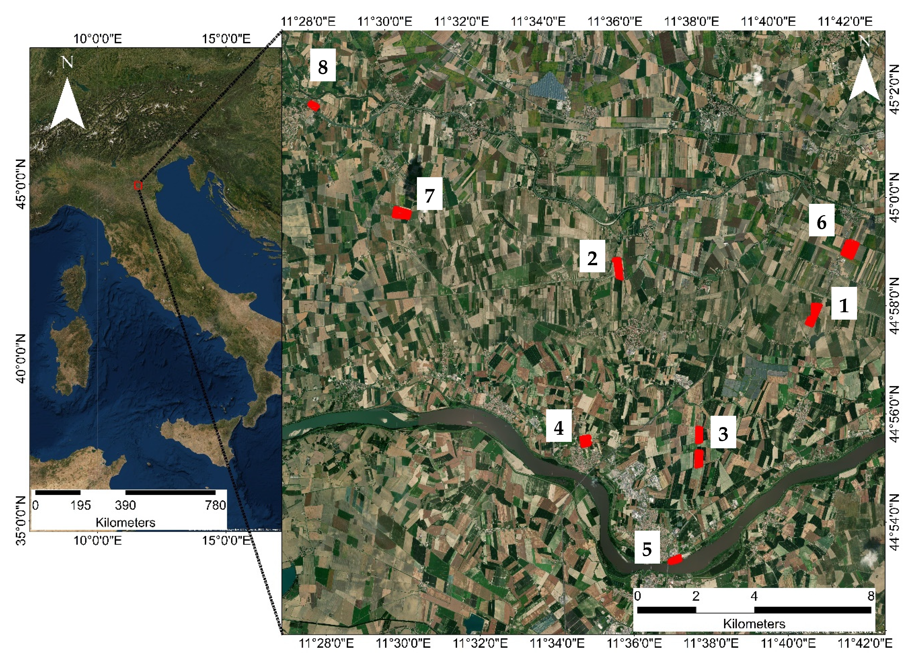
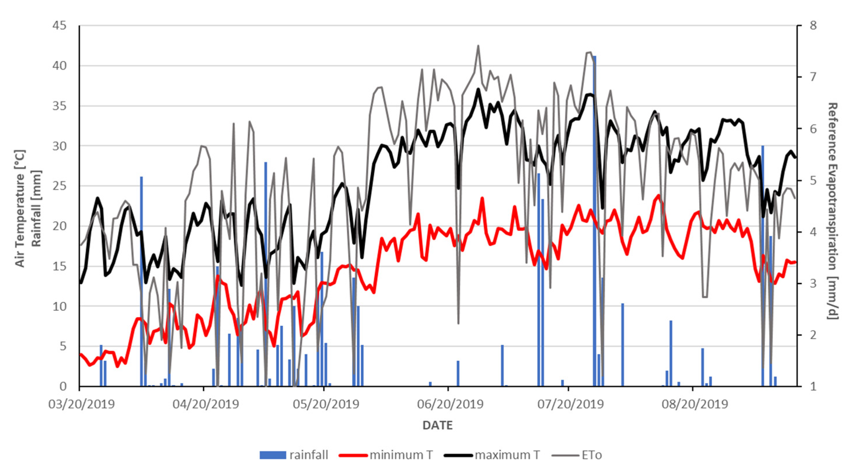
2.1. Study Fields, Weather Data, and Soil Characterization

The experiment was conducted in 2019 in eight distinct fields for approximately 90 ha located across the low plain of Veneto, Northeast Italy (Figure 1,

Table 1. Planting, Fertilization, Irrigation and Harvest dates for all the study fields. Damaged fields are labeled as D, whereas not damaged fields are marked as ND. * Irrigation events are expressed as total irrigation events and water volumes (in m³/ha).

Field ID	FAO Class	Planting Date	Fertilization	Irrigation *	Harvest
Field 1; D	500	03/29/19	270 N; 100 P2O5	3; 450	09/04/19
Field 2; D	500	03/28/19	170 N; 125 P2O5	N/A	08/28/19
Field 3; D	500	03/27/19	300 N; 184 P2O5	2; 500	09/02/19
Field 4; D	300	03/28/19	230 N; 185 P2O5	N/A	08/18/19
Field 5; D	300	03/28/19	230 N; 185 P2O5	N/A	08/18/19
Field 6; ND	500	03/27/19	295 N; 105 P2O5	1; 500	09/19/19
Field 7; ND	500	03/28/19	230 N; 80 P2O5; 80 K2O	2; 450	09/14/19
Field 8; ND	300	03/28/19	265 N; 30 P2O5	2; 500	08/20/19

). The climate is sub-humid, with an annual rainfall of 746 mm. In the median year, rainfall is highest in autumn and lowest in winter. Temperatures increase from January (minimum average: −1.3 °C) to July (maximum average: 31.4 °C). The reference evapotranspiration (ETo) between planting and harvest is 875 mm, with an average peak equal to 6.4 mm day⁻¹ in July. ETo exceeds rainfall from May to October. According to the Soil Survey Staff (1998), soil in the experimental areas are mainly Fluvaquentic Endoaquepts, fine, mixed, calcareous, mesic and Aquic Haplustepts fine-silty, mixed mesic.

The 2019 season was characterized by a wet April, May and July, while June reported low rainfall (Figure 2). Precipitation totaled 435 mm between planting and harvest. Minimum and maximum temperatures ranged on average from 2.5 °C and 18.1 °C in March to 14.7 °C and 31.4 °C in July. Reference ETo totaled 875 mm.

Maize (Zea mays L.) seeds of different varieties from two distinct maturity groups (FAO 300 and FAO 500) were planted between 27 March and 29 March 2019, at 0.75 m inter-row spacing and seeding rate of 7.5 seeds m⁻² (Table 1). Five out of eight fields were damaged by hailstorms that occurred on 13 July 2019 (damaged; D), while the other three were not damaged (ND). Since different farmers managed the areas with different agronomic protocols, all the information on planting, fertilization, irrigation and harvest are reported in Table 1. All the fields were harvested between 18 August and 17 September 2019.

2.2. Soil Parameters, Plant Samples and Yield Maps

Disturbed soil samples were collected at five locations per field from two different layers (0–0.5 m and 0.5–0.8 m) for a total of 80 samples. Soil texture was determined using a Malvern Mastersizer 2000 (Malvern Instruments Ltd., Great Malvern, UK) laser particle size analyzer. Before analysis, samples were air-dried, sieved at 2 mm and shaken for 12 h at 200 rpm in a 2% sodium hexametaphosphate solution. Soil pH [21], organic carbon (SOC; samples sieved at 0.5 mm; [21]) total Kjeldahl nitrogen (TKN, [21]) were determined on soil samples bulked at 0–0.5 m and 0.5–0.8 m, for a total of 16 values.

Soil texture ranged from silty clay (Field 1) to silty-clay-loam (Field 3, 5, 6 and 7) and silty loam (Field 2, 4, 8) (Supplementary Materials). Soil reaction was sub-alkaline, with a pH that slightly increased by depth. SOC and TKN ranged from 0.59–1.80% and 0.07 to 0.20%, respectively, with an average C/N of 8. Relative high SOC was observed at the top layer of the finer soils.

Before harvest, biomass samples were collected on the exact five locations per field. Two 1 m² plots were destructively harvested, dried at 65 °C for 24 h in a forced-air oven to determine the total aboveground dry weight (kg DM ha⁻¹), grain dry weight (kg DM ha⁻¹) and harvest index (HI). Harvest index was calculated as (Equation (1)):

HI = grain dry weight/(grain dry weight + total above − ground dry weight)

(1)

Yield maps were collected using a Claas Lexion 760TT (CLAAS, Harsewinkel, Germany) at Field 4, 5, a John Deere S770 (John Deere, Moline, IL) at field 6 and a Case IH AF-9230 (CNH Industrial, London, UK) at field 1, 2, and 3. All the combines were equipped with a yield monitor and a differential global positioning system (DGPS). They had a 7.5 m header and collected yield data every 5 s on the Claas Lexion combine and every second on the John Deere and Case IH combines. Yield maps were not generated for field 7 and 8, and measured yield was estimated dividing the total grain weight by the field size (in hectares). Raw yield data were imported using SMS™ Advanced (AgLeader Technology, Ames, ID, USA), cleaned to exclude field-edge effect and combine maneuvers [22] and expressed as grain dry matter per hectare (t DM ha⁻¹). Yield data were resampled at 30 × 30 m by ordinary kriging analysis (ArcMap 10.1, ESRI, Redlands, CA, USA) to match the spatial resolution of the Surface Energy Balance Algorithm for Land (SEBAL) maps.

2.3. Field Survey for Hail Damage with the Insurance Company Method

Along with the biomass samples, field surveys were performed on the exact five sampling locations per field by the insurance company’s agents to determine hail-related crop losses and estimate crop hail damage (HD_insurance). HD_insurance was calculated as the lowest value between the insured production and the potential production minus the estimated obtainable yield. The insured production is defined as the amount of yield (in kg DM ha⁻¹) that the farmer has insured for the specific field. In contrast, the potential production is the estimated obtainable yield for a specific growing season without crop hail losses. The potential production was first estimated according to the methodological approach provided by [23] and later validated by the insurance agents personal experience, considering the seasonal weather trends and yield levels reached by similar maize cultivars in contiguous, non-damaged areas. It is an expert-dependent, subject to bias, and not spatial variability-sensitive approach, but this is the most commonly used method by insurance agents during field surveys.

The estimated obtainable yield is defined as the production verified for a specific growing season after the hailstorm event. The obtainable yield was estimated through manual samplings, collecting all the plants on a total of 10 m² areas on the five sampling locations considering the total number of plants per m⁻², total number of kernels per ear, and the average kernel weight.

Commonly, the insured production is equal to or lower than the potential production, so HD_insurance is calculated as follows (Equation (2)):

HD_insurance (kg ha⁻¹) = Potential Production − Obtainable Production

(2)

In some cases, there could be some additional crop losses not related to the hail events (i.e., drought stress, pest damage, etc.). For this reason, HD_insurance is adjusted, removing these effects. The HD_insurance is then converted into a percentage dividing the damage in kg ha⁻¹ by the lowest value between potential production and insured production as discussed above.

Five different HD_insurance values were determined for the five different locations in each field and later averaged to determine the average crop hail damage for the entire field.

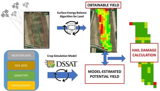
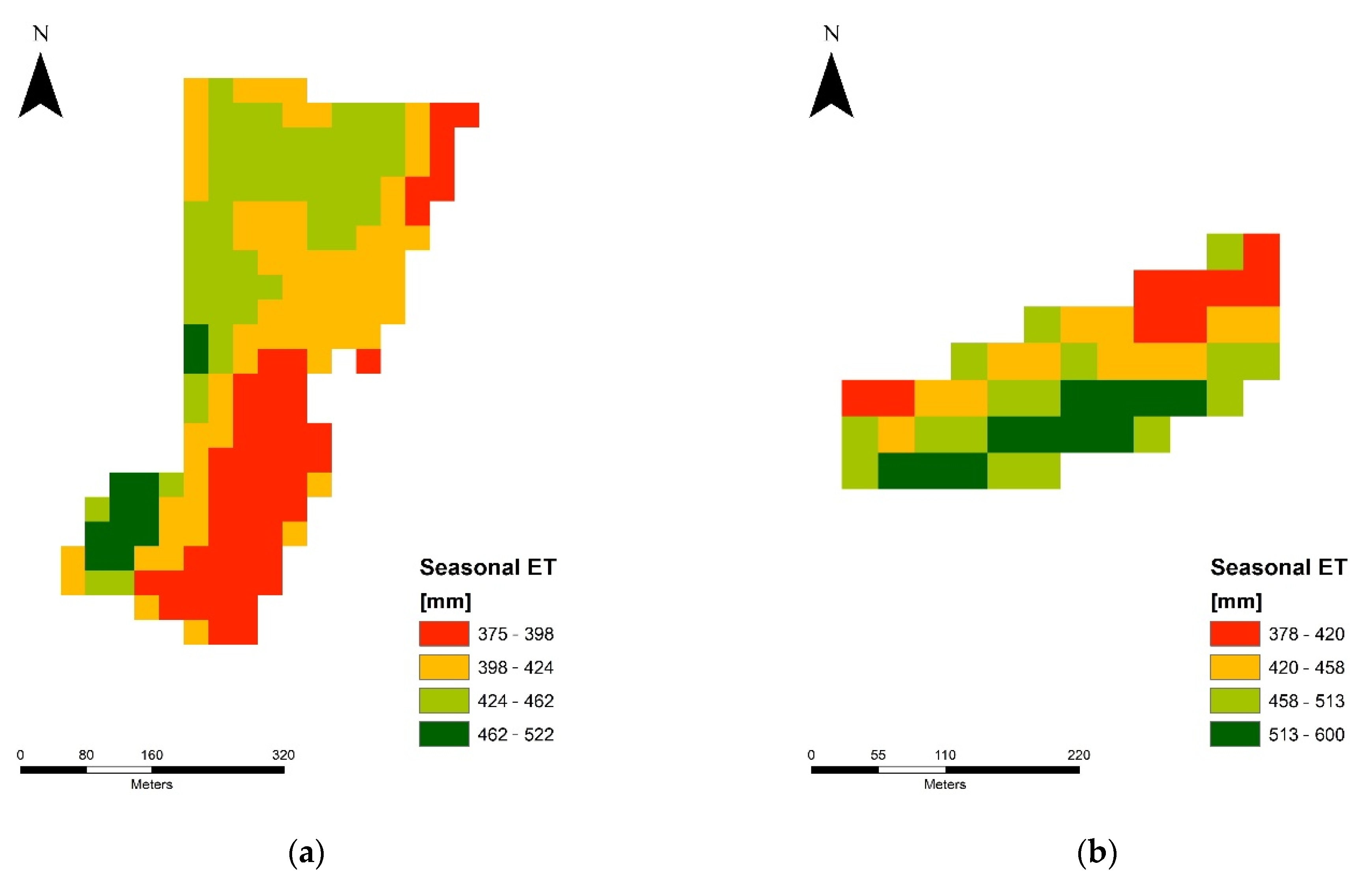
2.4. Seasonal ET, Actual Biomass and Yield Estimates Using the Surface Energy Balance Algorithm for Land (SEBAL)

The Surface Energy Balance Algorithm for Land (SEBAL) determines the actual evapotranspiration (ET_r) of each pixel by solving the energy balance equation (Equation (3); [24]):

$$\lambda E=R_n-G_0-H$$

(3)

where R_n is the net radiation, λE is the latent heat flux, G₀ is the soil heat flux, and H is the sensible heat flux. ET_r temporal integration was based on the calculation of j-th day fraction ETrF_j = ET_Sebal,j/ET_0,j (where j refers to the satellite image acquisition date and ET_0,j to the potential evapotranspiration for day j). ETrF_j, as an estimate of crop stress coefficient, was linearly interpolated for the period between two consecutive satellite images to compute the seasonal ET (termed ET_s) using the following equation:

$$E{T}_s={\displaystyle \sum }_j\left({\displaystyle \sum }_{i=t_j}^{t_{j+1}}E{T}_r{F}_{i}XET{o}_i\right)$$

(4)

where t_j and t_j+1 delimit a short period around the acquisition date j, ETrFi is the linearly interpolated evapotranspiration fraction at day i. Landsat 7 and 8 images from 30 March, 15 April, 30 April, 1 May, 16 May, 24 May, 1 June, 9 June, 18 June, 25 June, 3 July, 20 July, 4 August, and 20 August 2019 were downloaded and processed to calculate the energy balance components. All the selected images had favorable clear-sky weather conditions. Visible, NIRs and SWIRs bands (bands 1–5 and 7 for Landsat 7; 2–7 for Landsat 8) with a spatial resolution of 30 × 30 m were used for albedo (α), and NDVI calculations. Thermal band (band 6 for Landsat 7, and band 10 for Landsat 8) downscaled at 30 × 30 m were used to estimate surface temperature (T_s), and H. Atmospheric correction was performed to convert the top-of-atmosphere (TOA) radiance into surface reflectance using the second simulation of the satellite signal in the solar spectrum algorithm (6S) [25].

Maize total biomass accumulation (in kg DM ha⁻¹ day⁻¹) was calculated for all the satellite images using the fraction of absorbed photosynthetically active radiation (fPAR), the ETfr, and light use efficiency factor (e′) set at 4 g/MJ [24]. fPAR was estimated from NDVI values, as shown in Equation (5) [26]:

$$fPAR=-0.161+1.257\times NDVI$$

(5)

Total biomass (BIO) was converted into total aboveground biomass, excluding root biomass, as total biomass × 0.77. The formula assumes that root biomass represents approximately 23% of the total biomass at harvest (Equation (6); [25]).

$$\mathrm{total}\mathrm{aboveground}\mathrm{biomass} \left({\mathrm{kg}\mathrm{DM}\mathrm{ha}}^{-1}\right)=e^{\prime }\times ETfr\times fPAR\times 0.84\times 0.77$$

(6)

Maize yield was obtained by multiplying the total aboveground biomass for each pixel by the average HI calculated for each field from biomass samples, as discussed in 2.2 (Equation (1)). The field-to-field variability in HI was considered instead of using a flat HI value which often leads to over or underestimating the actual crop yield [26,27]. Moreover, model sensitivity to HI parameter was tested feeding the model with literature HI values (0.4, 0.45 and 0.5).

SEBAL-derived average yield values were then calculated for each field, except for field 8, and compared to the real yield averages determined with the yield maps at harvest. Relative percentage error was calculated for each pixel, comparing SEBAL and real yield averages (Equation (7)).

$$\mathrm{RELATIVE}\mathrm{ERROR}=\left|\frac{\left(\mathrm{REAL}\mathrm{YIELD}-\mathrm{SEBAL}\mathrm{YIELD}\right)}{\mathrm{REAL}\mathrm{YIELD}}\right|\times 100$$

(7)

2.5. The Decision Support System for Agrotechnology Transfer (DSSAT) Crop Model

The Decision Support System for Agrotechnology Transfer (DSSAT), CERES-Maize [28] crop model was used to simulate the potential yield (undamaged) of maize cultivars [29,30]. DSSAT simulates crop growth and development as a function of weather data, soil parameters, crop management, and genotype parameters. Soil parameters and crop management data, including planting date, density and depth, row spacing, fertilization and irrigation events, are reported in Table 1 and Supplementary Materials.

Genotype parameters include thermal time from seedling emergence to the end of the juvenile phase (P1), the extent to which development is delayed for each hour increase in photoperiod above the longest photoperiod at which development proceeds at a maximum rate (P2), thermal time from silking to physiological maturity (P5), the maximum number of kernels per plant (G2), kernel filling rate during the linear grain filling stage and under optimum conditions (G3), the interval in thermal time between successive leaf tip appearances (PHINT).

Minimum weather data required to run DSSAT, solar radiation (MJ m⁻²), minimum and maximum air temperature (°C) and daily precipitation (mm) during the 2019 growing season were provided by the Agenzia Regionale per la Prevenzione e Protezione Ambientale del Veneto (ARPAV) weather station (http://www.arpa.veneto.it/ (accessed on 1 November 2020)) located in Rovigo, Italy (45°02′00.3′′N, 11°49′33.5′′E).

2.5.1. Cultivar Calibration and Potential Yield Estimates Using DSSAT

The calibration procedure of the CERES-Maize was carried out running DSSAT in its sensitivity analysis tool. Starting for the default maize cultivar included in the DSSAT. CUL file, the two maize cultivars (FAO 300 and 500) were calibrated using yield data recorded during the 2019 season at harvest, soil data and weather data only for not damaged fields.

For the FAO 300 cultivar, the calibration was performed using yield data from one field, and the FAO 500 cultivar was calibrated using yield data recorded in two fields. The cultivars were manually calibrated, adjusting the aforementioned genotypic parameters (P1, P2, P5, G2 and G3). Simulated results were then compared to the observed yield. The genetic parameters were estimated through a trial-and-error, iterative approach to minimize the error between simulated and observed yield.

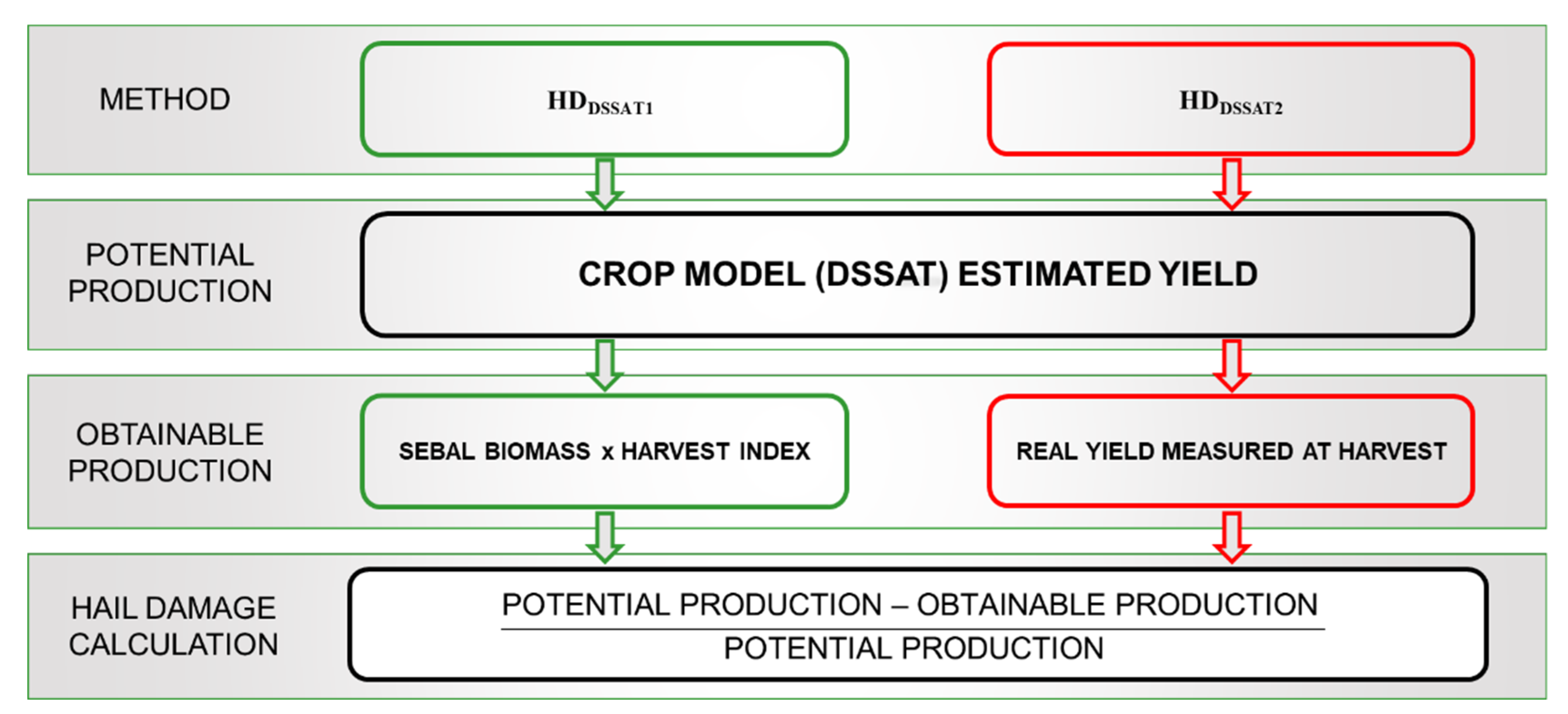
2.5.2. Estimates of Hail Damage with DSSAT and SEBAL-Based Methods

The DSSAT-calibrated FAO 300 and 500 cultivars were first used to estimate the five damaged fields’ potential yield, and later combined with the obtainable production using SEBAL (HD_DSSAT1) or real yields (HD_DSSAT2) Figure 3. The HD_DSSAT1 method was extended to estimate the potential production using HI values from the literature (0.40, 0.45, 0.50), hereafter labeled as HD_{DSSAT1_0.4}, HD_{DSSAT1_0.45}, and HD_{DSSAT1_0.5}.

Moreover, the HD_DSSAT1 calculation approach was extended to the literature HI values. These methods are labeled as HD_{DSSAT1_0.4}, HD_{DSSAT1_0.45}, and HD_{DSSAT1_0.5}. All the methodologies were compared to the HD_insurance to estimate differences between the methods. Hail damage was calculated from the DSSAT-estimated potential yields as in Figure 3.

3. Results

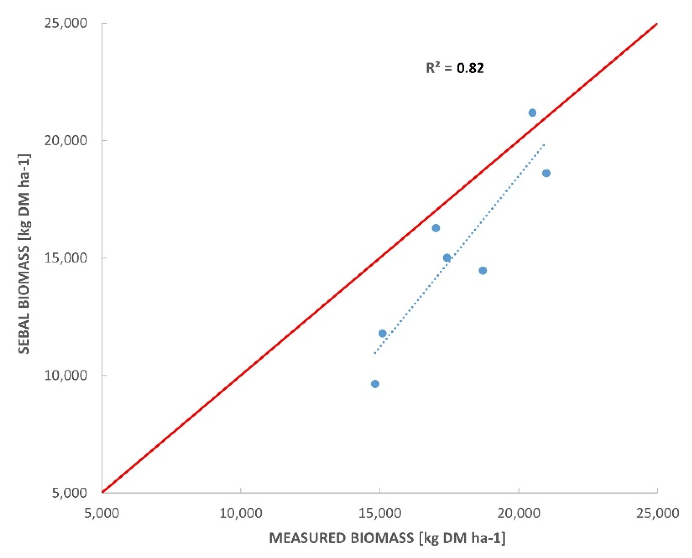
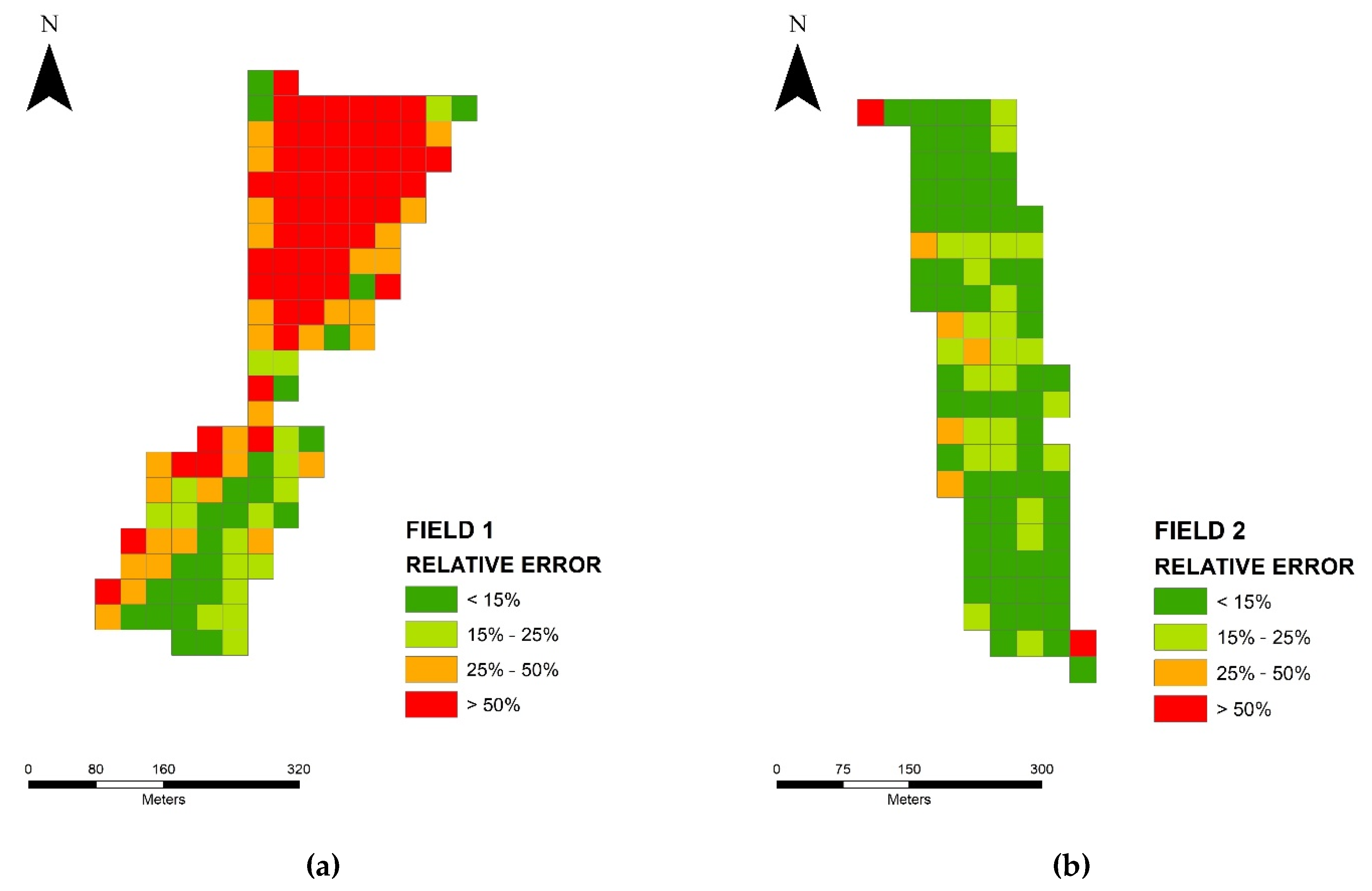
3.1. SEBAL-Based vs. Measured Biomass and Yield Estimates

Measured biomass showed high spatial variability, both within damaged and not damaged fields, varying from 14.8 to 21.0 t DM ha⁻¹ and a coefficient of variation (CV, expressed as%) ranging from a minimum of 1.3% (Field 4) to a maximum of 23.2% (field 5). Except for field 4, all the other fields had CV higher than 12%. The harvest index (HI), exhibited remarkable in- variability in field 2 (mean and CV of 0.53 and 19.0%), field 3 (mean and CV of 0.62 and 17.6% ) and field 5 (mean and CV of 0.40 and 27.8%). On the contrary, the variability was lower in field 1 (mean and CV of 0.54 and 8.2%) and field 4 (mean and CV of 0.48 and 3.7%) and not damaged fields 6 (mean and CV of 0.51 and 5.4%) and field 7 (mean and CV of 0.62 and 7.4%). Measured yield at harvest mirrored the total biomass results, ranging on average from 6.0 t DM ha⁻¹ (field 1) to 11.9 t DM ha⁻¹ (field 7).

Seasonal ET (ET_S) maps of the damaged fields calculated by SEBAL highlighted large in-field and field-to-field variability (Figure 4). Seasonal ET ranged from 282 mm (field 4) to 471 mm (field 5), with lower variability in field 1 (CV = 6.9%), field 2 (CV = 3.8%), and field 4 (CV = 8.2%) and higher in field 3 (CV = 14.0%) and 5 (CV = 12.0%).

The fraction ETrF_j ranged from a minimum average of 0.64 in field 4 to a maximum of 1.15 in field 5. Moderate variability was observed for all the investigated fields, with a coefficient of variation ranging between 3.6% (field 2) and 10.1% (field 3).

SEBAL-based algorithm well predicted the biomass at the two undamaged fields (field 6 and 7. SEBAL biomass was not calculated for field 8), with an average error of −4.0%, but underestimated (on average, −19.3%) biomass in most of the damaged fields with differences up to 35.0% as the maximum observed at Field 4. Considering all the damaged and undamaged fields, SEBAL underestimated the actual biomass by 15.1% (Figure 5).

SEBAL-based yields, calculated using literature HI (0.4, 0.45 and 0.5) values, are shown in

Table 2. Comparison between measured yield and SEBAL-estimated yield using the actual (SEBAL HI_real) and literature harvest index (SEBAL HI_0.4, SEBAL HI_0.45, SEBAL HI_0.5). Values in parenthesis represent the relative error from the measured yield at harvest. NC identifies not calculated SEBAL values.

Field ID	Measured Yld [t DM ha−1]	SEBAL HIreal [t DM ha−1]	SEBAL HI0.4 [t DM ha−1]	SEBAL HI0.45 [t DM ha−1]	SEBAL HI0.5 [t DM ha−1]
Field 1, D	6.01	7.81 (30.0)	5.79 (3.7)	6.51 (8.3)	7.23 (20.3)
Field 2, D	6.33	6.25 (1.3)	4.72 (25.5)	5.31 (16.2)	5.90 (6.9)
Field 3, D	9.17	9.31 (1.5)	6.01 (34.5)	6.76 (26.3)	7.51 (18.1)
Field 4, D	8.36	4.63 (44.6)	3.86 (53.9)	4.34 (48.1)	4.82 (42.3)
Field 5, D	6.28	6.51 (3.7)	6.51 (3.7)	7.32 (16.6)	8.14 (29.6)
Field 6, ND	9.16	10.80 (17.9)	8.47 (7.5)	9.53 (4.0)	10.59 (15.6)
Field 7, ND	11.90	11.46 (3.7)	7.44 (37.5)	8.37 (29.7)	9.30 (21.8)
Field 8, ND	10.70	NC	NC	NC	NC

. The relative errors calculated using the actual HI for damaged, not damaged, and all (damaged+not damaged) were, by far, the lowest. In fact, SEBAL-derived yield calculated using the actual HIs performed better than all the literature value-fed approaches with an average relative error of 10.8% for not damaged fields, 16.2% for damaged fields, and 14.7% combining damaged and not damaged fields.

Relative yield errors generated by SEBAL and yield map comparison presented high spatial variability (Figure 6, Supplementary Materials). The average relative error ranged from a minimum of 13.4% for field 2 to a maximum of 81.6% for field 4. High spatial variability was observed in fields 1, 4, and 5, with a standard deviation of 42.7%, 33.0%, and 54.0%. Field 2, 3, and 5 presented lower spatial variability with a standard deviation between 11.5% and 19.8%. Relative yield maps were not generated for field 7 and 8, since these fields were harvested without a yield-mapping system.

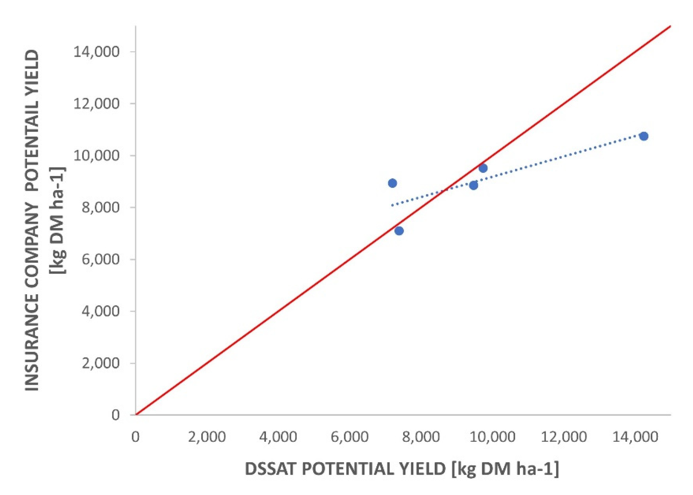
3.2. DSSAT Calibration and Potential Yield Estimates

The calibrated DSSAT well represented the measured yield for the not damaged fields. Measured and simulated yield averaged 9.1 t and 8.5 DM ha⁻¹ for field 6, 11.9 and 12.3 t DM ha⁻¹ for field 7, and 10.7 and 11.3 t DM ha⁻¹ for field 8.

After calibration, DSSAT was used to simulate the potential yield for the damaged fields and compared with the potential yields estimated by the insurance agents (Figure 7). On average, DSSAT potential yields resulted slightly higher (+5.2%) than the insurance company’s values. However, significant differences were observed for field 3 and field 5, being DSSAT predicting +32.4% in the former and −19.6% in the latter compared to insurance estimates).

3.3. Comparison of the Hail Damage Approaches

The HD_insurance, HD_DSSAT1, and HD_DSSAT2 methods presented similar values for fields 2, 3 and 5, while remarkable differences were observed for Field 1 and 4 (Table 2). In field 1, the use of the DSSAT crop simulation model and the insurance method led to similar potential yield estimates (9.74 vs. 9.52 t DM ha⁻¹). However, the measured yield was sensibly lower than the SEBAL and insurance agents’ estimates of obtainable yield. For this reason, the resulting HD_DSSAT2, using real yields, was higher (38.3%) than the other two approaches (HD_insurance = 22.8%; HD_DSSAT1 = 19.8%). Even in field 4, the SEBAL-estimated obtainable yield was notably lower than the measured yield and insurance company’s estimates (4.6 vs. 8.4 and 7.7 t DM ha⁻¹). The resulting HD_DSSAT1 was more than four times higher than the HD_insurance and HD_DSSAT2 (51.1% vs. 13.0% and 11.7%, respectively). On average, hail damage totaled 19.3%, 26.1%, and 22.5% for the HD_insurance, HD_DSSAT1, and HD_DSSAT2, respectively (

Table 3. Percentage hail damage estimates calculated for the different methodologies.

Field	HDInsurance	HDDSSAT1	HDDSSAT2	HDDSSAT1_0.4	HDDSSAT1_0.45	HDDSSAT1_0.5
	[%]	[%]	[%]	[%]	[%]	[%]
FIELD 1	22.8	19.8	38.3	40.6	33.2	25.7
FIELD 2	20.2	15.3	14.2	36.1	28.1	20.1
FIELD 3	30.8	34.6	35.6	57.8	52.5	47.3
FIELD 4	13.0	51.1	11.7	59.2	54.2	49.1
FIELD 5	9.9	9.5	12.7	9.5	0.0	0.0
AVERAGE	19.3	26.1	22.5	40.7	33.6	28.4

).

4. Discussion

In the current study, we supported the hypothesis that the integration of remote sensing and crop modeling would allow the definition of a novel, robust and objective approach to quantify hail damage on maize. While methods based on NDVI differences of pre and post-hailstorm events are highly influenced by spatial resolution, available images, and sensing period [7,18], the presented methodology, despite the limited number of investigated fields, provides objective hail damage estimates, integrating crop simulation models and the Surface Energy Balance Algorithm for Land.

SEBAL biomass estimates well agreed to in-field sampled biomass for the not damaged fields (−4%), whereas more significant differences were observed for the damaged fields with an average underestimation of 15%. This underestimation could be related to the different support size used in the two approaches, 30 m × 30 m for SEBAL and 2 m² for the hand-harvested samples, whose differences were exacerbated in heterogeneous canopy conditions such as those of damaged fields.

Similarly, the use of heterogeneous estimated HIs across fields has led to a better performance in SEBAL-derived yields than all the literature value-fed approaches. The excellent performance of the SEBAL-based model agrees with previous research findings on maize crop in the same area [26,27]. Nevertheless, some error peaks close to 40% observed in a few areas were most likely related to under or overestimating the actual harvest index. In this case, these differences could not be related to the different support size of the methods since SEBAL-based and measured yield maps were compared at the same spatial resolution of 30 × 30 m. Using the average of the five measured HI values per field could be misleading. HI was shown to have a large spatial variability even within small areas [31]. The large spatial variability in errors between SEBAL and real yield values (Figure 6) highlights the strong in-field variability in hail damage responses. These differences could be presumably linked to in-field differences in harvest index.

These findings reinforce the need for a tool that estimates, on a spatial scale, harvest index as a function of crop stresses. It could represent a viable alternative to provide more accurate SEBAL-based yield estimates, especially for those under non-optimal conditions [32].

The good cultivar calibration obtained with the crop simulation model represents a promising result, given the minimum number of undamaged fields involved in the calibration procedure (one for the FAO 300 and two for the FAO 500 cultivar). Performing the cultivar calibration on a larger dataset, including more combinations of climate and soils, would undoubtedly provide greater robustness to the model.

DSSAT potential yield estimates of damaged fields resulted slightly higher (on average +5.2%) than the insurance company’s values. These under and overestimations could be related to the insurance company’s sampling methodology, based on scouting of small survey areas coupled with the insurance agent experience. While agents provide potential yield estimates based on their experience and samples that are not always representative of the examined area and weather conditions, using an objective tool as a crop simulation model would improve the field survey procedure [7].

The comparison between the different hail damage approaches provided some interesting points. The insurance company’s hail damage method (HD_insurance) averaged 3.2% less than the reference method (HD_DSSAT2), and the novel approach (HD_DSSAT1) slightly overestimated (+3.6%) the reference hail damage. However, the three methods had similar estimates for most investigated fields, and most of the differences were observed in fields 1 and 4. These differences were related to SEBAL-based estimates of obtainable yield for the aforementioned fields (Figure 4), suggesting the need to improve the biomass accumulation algorithm.

5. Conclusions

In the present study, the SEBAL-based estimates of biomass and crop yield over 90 hectares were integrated with crop models to define a novel, objective and less labor-intensive hail damage assessment approach. Results were compared to hail damage estimates from the insurance company and to our reference method.

Hail damage estimates from the proposed method largely agreed to the estimates from the reference method and the insurance company. Some differences were observed between the methods, probably related to inaccurate SEBAL estimates of obtainable yield. Additionally, the poor performance of hail damage methodologies fed with literature HI values suggested the importance of quantifying the spatial variability in the harvest index for accurate yield estimates. The results suggest the integration of remote sensing platforms (for determining the obtainable yield) and crop models (for potential yield estimates in hail damaged fields) could be successfully employed for the definition of a novel and reliable method able to quantify crop hail damage. However, more robust estimates of the potential yield are required by calibrating models on a larger dataset, including different soil and weather conditions. Using a model able to determine the spatial variability in harvest index as a function of crop stress is necessary to improve SEBAL yield estimates’ accuracy and the resulting calculated percentage of hail damage.

The adoption of remote-sensing-based crop insurance methods has great promises for the insurance market. More robust and less time-consuming methodologies will enable insurance companies to extend their markets and change how this business is done.

A major limitation of this work is the limited number of investigated fields. Further studies will be necessary to validate the proposed methodology over different experimental areas and a broader range of hail damage intensity.

References

1. Baldi, M.; Ciardini, V.; Dalu, J.D.; De Filippis, T.; Maracchi, G.; Dalu, G. Hail occurrence in Italy: Towards a national database and climatology. Atmos. Res. 2014, 138, 268–277. [Google Scholar] [CrossRef]
2. Politeo, M. I Danni da Grandine Sulle Colture Agrarie del Veneto dal 1990 al 2004. Ph.D. Thesis, University of Padua, Padua, Italy, 2008. [Google Scholar]
3. Kunz, M.; Blahak, U.; Handwerker, J.; Schmidberger, M.; Punge, H.J.; Mohr, S.; Fluck, E.; Bedka, K.M. The severe hailstorm in southwest Germany on 28 July 2013: Characteristics, impacts and meteorological conditions. Q. J. R. Meteorol. Soc. 2018, 144, 231–250. [Google Scholar] [CrossRef]
4. Schuster, S.S.; Blong, R.J.; Speer, M.S. A hail climatology of the greater Sydney area and New South Wales, Australia. Int. J. Climatol. A J. R. Meteorol. Soc. 2005, 25, 1633–1650. [Google Scholar] [CrossRef]
5. Changnon, S.A. Increasing major hail losses in the US. Clim. Chang. 2009, 96, 161–166. [Google Scholar] [CrossRef]
6. Wang, E.; Bertis, B.L.; Jimmy, R.W.; Yu, Y. Simulation of hail effects on crop yield losses for corn-belt states in USA. Trans. Chin. Soc. Agric. Eng. 2012, 28, 177–185. [Google Scholar]
7. Young, F.R.; Apan, A.; Chandler, O. Crop hail damage: Insurance loss assessment using remote sensing. In Proceedings of the Annual Conference of the Remote Sensing and Photogrammetry Society, Aberdeen, UK, 7–10 September 2004. [Google Scholar]
8. Manzato, A. Hail in northeast Italy: Climatology and bivariate analysis with the sounding-derived indices. J. Appl. Meteorol. Climatol. 2012, 51, 449–467. [Google Scholar] [CrossRef]
9. Punge, H.J.; Bedka, K.M.; Kunz, M.; Werner, A. A new physically based stochastic event catalog for hail in Europe. Nat. Hazards 2014, 73, 1625–1645. [Google Scholar] [CrossRef]
10. Mohr, S.; Kunz, M.; Keuler, K. Development and application of a logistic model to estimate the past and future hail potential in Germany. J. Geophys. Res. Atmos. 2015, 120, 3939–3956. [Google Scholar] [CrossRef]
11. Morgan, G.M., Jr. A general description of the hail problem in the Po Valley of northern Italy. J. Appl. Meteorol. Climatol. 1973, 12, 338–353. [Google Scholar] [CrossRef] [Green Version]
12. Eldredge, J.C. The effect of injury in imitation of hail damage on the development of the maize plant. Iowa Agric. Home Econ. Exp. Stn. Res. Bull. 1935, 16, 1. [Google Scholar]
13. Shapiro, C.A.; Peterson, T.A.; Flowerday, A.D. Yield Loss Due to Simulated Hail Damage on Corn: A Comparison of Actual and Predicted Values. Agron. J. 1986, 78, 585–589. [Google Scholar] [CrossRef]
14. Vorst, J.J. Assessing Hail Damage to Corn; Iowa State University Extension: Ames, IA, USA, 1991. [Google Scholar]
15. Towery, N.G.; Eyton, J.R.; Changnon, S.A., Jr.; Dailey, C.L. Remote Sensing of Crop Hail Damage; Illinois State Water Survey: Champaign, IL, USA, 1975. [Google Scholar]
16. Erickson, B.J.; Johannsen, C.J.; Vorst, J.J.; Biehl, L.L. Using remote sensing to assess stand loss and defoliation in maize. Photogramm. Eng. Remote Sens. 2004, 70, 717–722. [Google Scholar] [CrossRef]
17. Peters, A.J.; Griffin, S.C.; Viña, A.; Ji, L. Use of remotely sensed data for assessing crop hail damage. PE&RS, Photogramm. Eng. Remote Sens. 2000, 66, 1349–1355. [Google Scholar]
18. Zhao, J.L.; Zhang, D.Y.; Luo, J.H.; Huang, S.L.; Dong, Y.Y.; Huang, W.J. Detection and mapping of hail damage to corn using domestic remotely sensed data in China. Aust. J. Crop Sci. 2012, 6, 101. [Google Scholar]
19. Zhou, J.; Pavek, M.J.; Shelton, S.C.; Holden, Z.J.; Sankaran, S. Aerial multispectral imaging for crop hail damage assessment in potato. Comput. Electron. Agric. 2016, 127, 406–412. [Google Scholar] [CrossRef] [Green Version]
20. De Leeuw, J.; Vrieling, A.; Shee, A.; Atzberger, C.; Hadgu, K.M.; Biradar, C.M.; Keah, H.; Turvey, C. The potential and uptake of remote sensing in insurance: A review. Remote Sens. 2014, 6, 10888–10912. [Google Scholar] [CrossRef] [Green Version]
21. Ministero delle Politiche Agricole e Forestali. Metodi ufficiali di analisi chimica del suolo. Decreto Ministeriale 13 settembre 1999. In Supplemento Ordinario Alla Gazzetta Ufficiale n°248 del 21 Ottobre 1999; Ministero delle Politiche Agricole e Forestali: Rome, Italy, 1999. [Google Scholar]
22. Vega, A.; Córdoba, M.; Castro-Franco, M.; Balzarini, M. Protocol for automating error removal from yield maps. Precis. Agric. 2019, 20, 1030–1044. [Google Scholar] [CrossRef]
23. Nicoli, L. Procedure per la Stima dei Danni da Avversità Atmosferiche; Veneto Agricoltura: Legnaro, Italy, 2019. [Google Scholar]
24. Bastiaanssen, W.G.; Menenti, M.; Feddes, R.A.; Holtslag, A.A.M. A remote sensing surface energy balance algorithm for land (SEBAL). 1. Formulation. J. Hydrol. 1998, 212, 198–212. [Google Scholar] [CrossRef]
25. Vermote, E.F.; Tanré, D.; Deuze, J.L.; Herman, M.; Morcette, J.J. Second simulation of the satellite signal in the solar spectrum, 6S: An overview. IEEE Trans. Geosci. Remote Sens. 1997, 35, 675–686. [Google Scholar] [CrossRef] [Green Version]
26. Grosso, C.; Manoli, G.; Martello, M.; Chemin, Y.H.; Pons, D.H.; Teatini, P.; Piccoli, I.; Morari, F. Mapping maize evapotranspiration at field scale using SEBAL: A comparison with the FAO method and soil-plant model simulations. Remote Sens. 2018, 10, 1452. [Google Scholar] [CrossRef] [Green Version]
27. Gobbo, S.; Lo Presti, S.; Martello, M.; Panunzi, L.; Berti, A.; Morari, F. Integrating SEBAL with in-Field Crop Water Status Measurement for Precision Irrigation Applications—A Case Study. Remote Sens. 2019, 11, 2069. [Google Scholar] [CrossRef] [Green Version]
28. Jones, C.A. CERES-Maize: A Simulation Model of Maize Growth and Development (No. 04; SB91. M2, J6.); Texas A&M University Press: College Station, TX, USA, 1986. [Google Scholar]
29. Jones, J.W.; Hoogenboom, G.; Porter, C.H.; Boote, K.J.; Batchelor, W.D.; Hunt, L.A.; Wilkens, P.W.; Singh, U.; Gijsman, A.J.; Ritchie, J.T. The DSSAT cropping system model. Eur. J. Agron. 2003, 18, 235–265. [Google Scholar] [CrossRef]
30. Hoogenboom, G.; Jones, J.; Wilkens, P.; Porter, C.; Boote, K.; Hunt, L.D.; Singh, U.; Lizaso, J.I.; White, J.M.; Uryasev, O.; et al. Decision Support System for Agrotechnology Transfer (DSSAT) Version 4.5; Honolulu University: Honolulu, HI, USA, 2010; Volume 1. [Google Scholar]
31. Zwart, S.J.; Bastiaanssen, W.G. SEBAL for detecting spatial variation of water productivity and scope for improvement in eight irrigated wheat systems. Agric. Water Manag. 2007, 89, 287–296. [Google Scholar] [CrossRef]
32. Scudiero, E.; Teatini, P.; Corwin, D.L.; Ferro, N.D.; Simonetti, G.; Morari, F. Spatiotemporal response of maize yield to edaphic and meteorological conditions in a saline farmland. Agron. J. 2014, 106, 2163–2174. [Google Scholar] [CrossRef] [Green Version]
Figure 1. Aerial image of the study fields (Esri, 2019) with numbers indicating the different experimental areas discussed in Table 1.
Remotesensing 13 02655 g001
Figure 2. Daily maximum (black line), minimum (red line) air temperature, reference DSSAT evapotranspiration (gray line), and rainfall (blue vertical bars) during the 2019 growing season from the Agenzia Regionale per la Prevenzione e Protezione Ambientale del Veneto (ARPAV; http://www.arpa.veneto.it/, accessed on 1 July 2021) weather station in Rovigo.
Remotesensing 13 02655 g002
Figure 3. Overview of the calculation steps performed for the investigated DSSAT and SEBAL-based methods.
Remotesensing 13 02655 g003
Figure 4. SEBAL seasonal ET maps generated for Field 1 (a) and Field 5 (b).
Remotesensing 13 02655 g004
Figure 5. Comparison between measured aboveground biomass from hand-harvested plant samples (x axis) and SEBAL-estimated aboveground biomass (y axis) for all the different experimental areas. Values are expressed as kg DM ha−1. The 1:1 line is reported in red.
Remotesensing 13 02655 g005
Figure 6. Relative error maps generated for Field 1 (a) and Field 2 (b) between measured and SEBAL-estimated yields.
Remotesensing 13 02655 g006
Figure 7. DSSAT-estimated potential yield (x axis) and potential yield estimates from the insurance agents (y axis) for the five damaged fields. Values are expressed as kg DM ha−1. The 1:1 line is reported in red.
Remotesensing 13 02655 g007