Abstract
Hyperspectral remote sensing across multiple spatio-temporal scales allows for mapping and monitoring mangrove habitats to support urgent conservation efforts. The use of hyperspectral imagery for assessing mangroves is less common than for terrestrial forest ecosystems. In this study, two well-known measures in statistical physics, Mean Information Gain (MIG) and Marginal Entropy (ME), have been adapted to high spatial resolution (2.5 m) full range (Visible-Shortwave-Infrared) airborne hyperspectral imagery. These two spectral complexity metrics describe the spatial heterogeneity and the aspatial heterogeneity of the reflectance. In this study, we compare MIG and ME with surface reflectance for mapping mangrove extent and species composition in the Sierpe mangroves in Costa Rica. The highest accuracy for separating mangroves from forest was achieved with visible-near infrared (VNIR) reflectance (98.8% overall accuracy), following by shortwave infrared (SWIR) MIG and ME (98%). Our results also show that MIG and ME can discriminate dominant mangrove species with higher accuracy than surface reflectance alone (e.g., MIG–VNIR = 93.6% vs. VNIR Reflectance = 89.7%).
1. Introduction
Mangroves are considered to be among the most threatened ecosystems on Earth [1], despite their ecological and economical importance. Globally, mangroves cover 137,760 km2 [2] and are estimated to be disappearing at a rate of approximately 1% annually, primarily caused by human alteration to the landscape [1,3]. Conversion of mangrove habitats to agriculture, aquaculture, urbanization, and their over-exploitation are among the leading causes for their loss and there is an urgent need for conservation and restoration [1,4,5]. Structurally, mangroves are characterized by a unique composition of tree and shrub species capable of thriving in saline conditions [4]. They are primarily found in coastal environments in the tropical and subtropical regions of the world, forming an interface between the sea and terrestrial environment [6,7]. They serve as an important ecological and economic resource providing many ecosystem services [8,9,10]. For instance, mangroves serve both as a barrier that protects coastlines and as significant carbon sinks (blue carbon) [11], thus serving as a key natural climate solution to mitigate global warming [4,12]. The structural complexity of mangrove forests makes them highly efficient in trapping laterally imported carbon from riverine and oceanic sources [11]. It has therefore become increasingly important to monitor the periodic changes of their extent and distribution to assist in conservation planning [13]. However, the inundation and inaccessibility that regularly characterizes mangroves makes it extremely challenging to conduct field observations using conventional survey methods [9]. The cost, logistics, and time investment required for such field observations are often deemed impractical and a major concern to ecologists, particularly when considering data collection over a large spatial extent [14]. Remote sensing has shown great promise in overcoming these constraints (e.g., [2,15]).
Until recently, the primary utility of remote sensing has been to map mangrove extent at different scales [6,9,16], predominantly from moderate spatial resolution (i.e., ≥10 m) satellite imagery such as Sentinel-2 [17,18]. The Global Mangrove Distribution map was developed based on Landsat imagery [2], and, subsequently, Global Mangrove Watch (GMW) produced an updated global baseline map of mangrove extent using a combination of Synthetic Aperture Radar (SAR) data acquired by the Advanced Land Observing Satellite (ALOS) Phased-Array L-band Synthetic Aperture Radar (PALSAR) and a composite of Landsat imagery [19]. Despite the promising results attained by the ALOS PALSAR products, they depend on flooding of mangrove habitats for optimal performance. Seasonally flooded mangroves may result in sub-optimal mangrove classification performance and the 1 ha spatial constraints of ALOS PALSAR products makes it difficult to accurately detect smaller fragmented areas of mangroves [19]. Therefore, a high spatial resolution optical image mapping approach is still needed to delineate fragmented mangrove areas.
Mangrove species have also been mapped using data from Earth observation satellites and manned and unmanned aerial systems across multiple spatio-temporal scales. For instance, multispectral imagery acquired from the Landsat series, Sentinel-2, and SPOT have been used for mapping species composition [6,9]. Mangrove species were also mapped successfully by extracting image texture and spectral statistics from IKONOS and Quickbird multispectral imagery, with IKONOS showing superior results [20]. However, due to limitations in spectral resolution, conventional satellite imagery is somewhat restricted in its ability to effectively separate mangrove species [15].
The limitations of multispectral satellite imagery can impact mangrove classification accuracy [6,15]. Hyperspectral imagery (HSI) can overcome these constraints and potentially attain better classification results. HSI is characterized by substantially higher spectral resolution compared to conventional multispectral sensors. The predominant features often used to discriminate mangrove communities using HSI are mainly spectral characteristics (both at canopy and leaf levels) as well as texture [21,22]. Pixel based supervised classification methods and machine learning techniques (e.g., maximum likelihood, support vector machine, random forest classification, etc.) that utilize the spectral characteristics of materials have dominated studies involving mangrove classification [9,23]. For instance, mangrove species mapping based on the spectral angle from Hyperion imagery attained an overall classification accuracy of 76.4% [24]. Mangrove habitats have also been mapped with airborne HSI using three different methods (i.e., band ratio, supervised and unsupervised classification) with resultant accuracies between 70–85%, higher than the classification accuracy attained with SPOT and Landsat multispectral imagery of the same study area [15]. Additionally, the use of object-based image analysis more accurately discriminated species (Overall Accuracy (OA) = 76%) than a pixel-based approach (OA = 56%) from airborne HSI (spatial resolution = 4 m) [25]. By incorporating a digital surface model with object-based analysis of UAV-HSI (spatial resolution = 2 cm), the classification accuracy of mangrove species improved by approximately 6% (OA = 82.09% vs. 88.66%) [22]. Nonetheless, virtually all classification methods are affected by the spectral variability in HSI [26]. Therefore, for optimal classification performance or target detection, an understanding of the spectral variability is required to ensure the approach chosen is robust to the inherent spectral variability captured by HSI [26].
Although HSI has been shown to be very promising, the development of methods that advance HSI analysis to assist in mapping mangrove extent and species composition is in the initial stages [9]. Continued development of more reliable and robust techniques for rapid assessment of vegetation at multiple spatial scales has been encouraged for conservation planning [27]. Recently, there have been substantial research efforts concentrating on the development of methods for quantifying ecosystem structural complexity [28]. For instance, spatial and aspatial measures of complexity known as the Mean Information Gain (MIG) and Marginal Entropy (ME) derived from a single band of RGB photographs (from digital cameras) have been developed for rapid assessments of ecosystems [28,29]. MIG is a measure of the randomness of a given landscape, considering the spatial variation in reflected radiation across the landscape. In other words, MIG provides an estimate of the spatial heterogeneity of the reflectance in the landscape being studied. In contrast, ME (i.e., Shannon Entropy) provides an estimate of aspatial spectral heterogeneity, which is the probability of observing a pixel value independent of its location in the scene [30]. Several studies have demonstrated the utility of these metrics for biodiversity assessments, with promising results. For instance, an empirical relationship was established between MIG estimated from digital photographs and benthic epibiota richness and evenness [27], and MIG computed from digital photographs and satellite imagery has been linked to habitat complexity of a coral reef [31]. Similarly, a positive relationship was established between biodiversity metrics of understory vegetation in a temperate forest and MIG and ME derived from digital RGB photographs [30,32]. Despite the promising results attained in these studies, MIG and ME metrics have not yet been applied to HSI for mangrove forest extent and species mapping. The MIG and ME adapted to HSI are referred to as spectral complexity metrics (SCM), where MIG is the spectral reflectance spatial heterogeneity (spectro-spatial heterogeneity) and ME is the spectral reflectance aspatial heterogeneity (aspatial spectral complexity) [28,33].
In this study, MIG and ME are applied to high spatial resolution (2.5 m) full range (Visible-Shortwave-Infrared) airborne hyperspectral imagery acquired over the Sierpe mangroves in southern Costa Rica. The three main objectives of our study are: (1) To determine the utility of the spectral complexity metrics (MIG and ME) for discriminating mangrove extent from terrestrial forest, (2) To compare the separability of predominant mangrove species using spectral complexity metrics and surface reflectance, and (3) To examine the spectral variability of the predominant mangrove species across the visible to shortwave infrared regions. It is expected that the results from this study will support landscape mapping of mangrove forest extent and species distribution to complement global mangrove conservation efforts.
2. Materials and Methods
2.1. Study Site
Our study focused on approximately 18,000 ha of mangrove forest in Sierpe, along the southwest Pacific coast of Costa Rica (Figure 1). The Térraba-Sierpe mangroves, as they are known in Costa Rica, are found in the estuary of the Rio Grande de Térraba and Rio Sierpe rivers [34]. This large mangrove ecosystem constitutes approximately 40% of all mangroves in the country. The adjacent old-growth tropical wet forest on the Osa peninsula is known for its high biodiversity. It is part of a large conservation area known as the Área de Conservación de Osa (ACOSA) [35,36] (Figure 2). Although the study area is considered to have undergone minimal disturbance compared to other similar habitats in Costa Rica, it is threatened due to anthropogenic activities and economic factors [37].
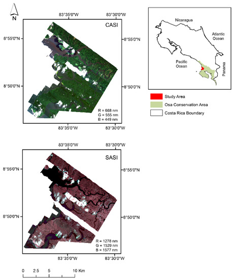
Figure 1.
Térraba-Sierpe mangrove forest ecosystem located on the Osa Peninsula, Costa Rica. The map contains two mosaics: A mosaic of imagery acquired with the Compact Airborne Spectrographic Imager–CASI 1500 (R = 668 nm G = 555 nm B = 449 nm) and a mosaic of imagery acquired with Shortwave Airborne Spectrographic Imager–SASI 644 (R = 1278 nm G = 1529 and B = 1577 nm).

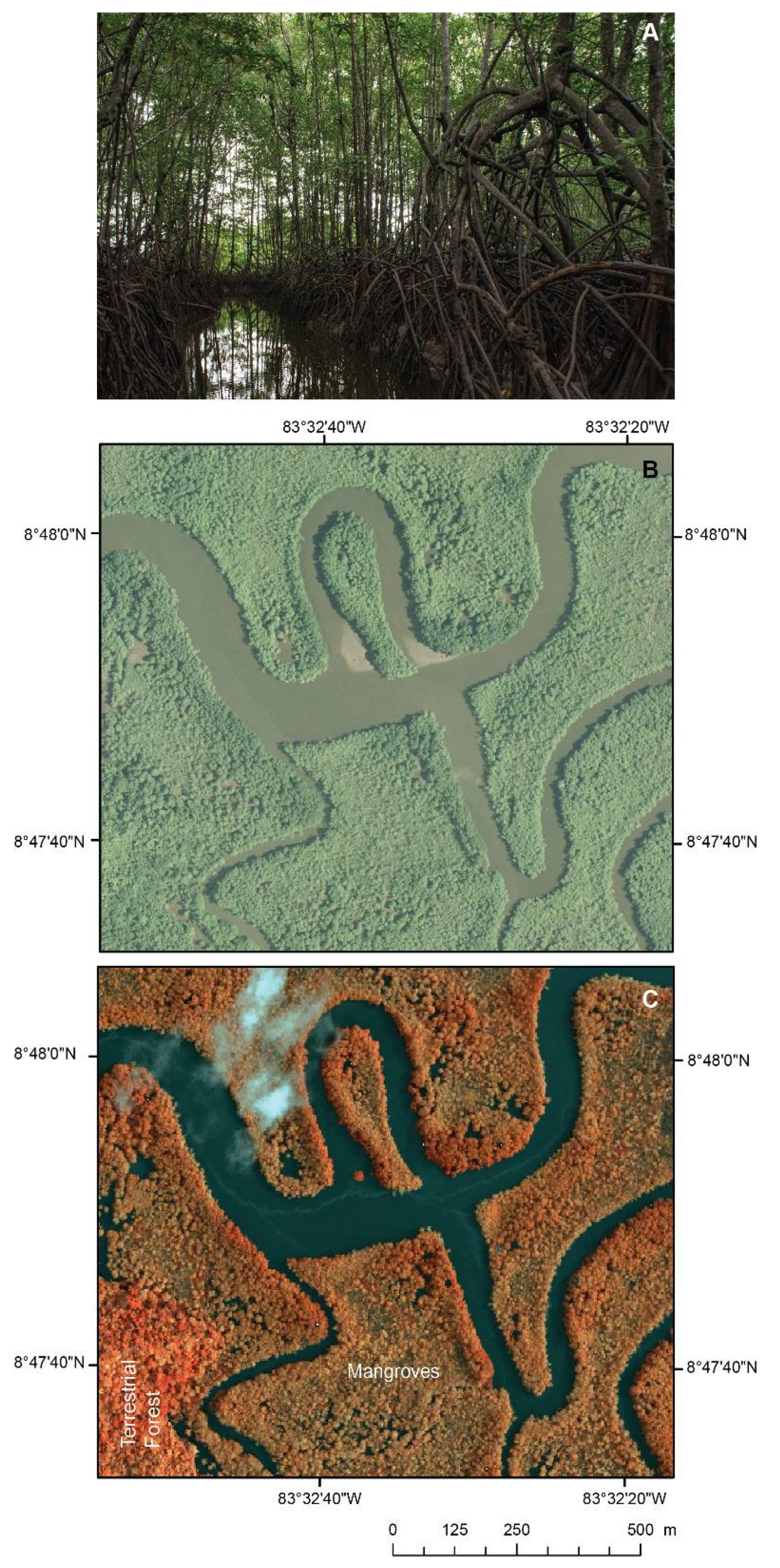
Figure 2.
(A) Ground photograph from the Sierpe mangroves, (B) Subset of the CARTA 2005 aerial photographs from the mangroves, (C) Subset of a CASI 1500 HSI (R: 748 nm G: 550 nm B: 519 nm) flight line acquired in 2013 illustrating the same subset of mangroves as seen in B. The delimitation of terrestrial forest and mangroves is more apparent from the HSI than from the aerial photograph.
Despite these ongoing threats, very few studies have attempted to map the recent status and extent of the mangroves on a landscape scale. Apart from global efforts to map overall mangrove extent [2,38], some large-scale mapping of mangrove extent was conducted two decades ago using moderate resolution (30 m) Landsat TM satellite imagery and SPOT-2 Imagery (60 m resolution) [39]. Although some recent landscape scale species distribution mapping efforts have also been conducted with RapidEye satellite imagery (e.g., [40]) and a combination of field surveys, aerial photographs from the Costa Rican Airborne Research and Technology Applications (CARTA) mission along with Quickbird imagery [41], continued temporal monitoring of mangrove extent and species distribution on a landscape scale is needed for conservation planning and decision making. The predominant species in Sierpe include Rhizophora racemosa (mangrove tree), Pelliciera rhizophorae (mangrove tree), Rhizophora mangle (mangrove tree) and Acrostichum aureum (fern) [40].
2.2. Airborne Hyperspectral Imagery (HSI)
We used airborne HSI acquired by Mission Airborne Carbon 2013 (MAC13) [42]. The imagery consists of data from two distinct pushbroom sensors, the Compact Airborne Spectrographic Imager 1500 (CASI) and the Shortwave Airborne Spectrographic Imager 644 (SASI). The CASI-1500 acquired 199 spectral bands across the 375 nm to 1050 nm wavelength range, while the SASI acquired 160 spectral bands across the 883 nm to 2523 nm range. Characteristics of the sensors and sample flight planning parameters are outlined in Table 1 and Table 2.

Table 1.
Characteristics of CASI-1500 and SASI-644 Sensors used in the Mission Airborne Carbon 2013 (MAC13) project for collecting HSI over the study area.
Table 2.
Sample flight planning parameters for the study region for both CASI and SASI modified from [42].
2.3. Pre-Processing
The raw images were preprocessed to radiance following the standard methodology described in [42,44]. The Atmospheric and Topographic correction module implemented in ATCOR-4 (rugged terrain) (Version 7.3.0 2019) was used to account for the influence of the atmosphere, terrain, solar illumination geometry, and viewing geometry of the sensor to derive surface reflectance. Although our study was focused on the mangroves, surrounding terrestrial forests were characterized by highly variable topographic complexity, with a mean elevation and standard deviation of 100 m and 119 m, representing an elevation range of 0–669 m [42]. Topographic differences are known to cause variability in the incident radiation [45]; as a result, bidirectional reflectance effects are inevitable, with potential implications on the quality of the spectral information [46]. This topographic influence traceable to individual pixels must be accounted for during the preprocessing stage to ensure consistency in the spectra [45,46]. The incident angle topographic BRDF effect was corrected using the Modified Minnaert (MM) topographic correction routine available in ATCOR-4 [46].
The low signal and noisy regions of the CASI (<400 nm and >900 nm) were excluded from further analysis. For the SASI, bands in the wavelength ranges between 1367 nm–1492 nm and 1800 nm–2200 nm were excluded from the analysis due to atmospheric water absorption and known low signal-to-noise ratio. Finally, because spectral artefacts tend to remain after atmospheric correction, particularly for high spectral resolution datasets [47], spectral polishing was applied in ATCOR-4 to reduce these residual artefacts. The final number of bands that remained for the CASI and SASI were 174 and 65, respectively. The parameters used for the atmospheric correction are shown in Table S1 (Supplementary Material).
After atmospheric correction, the flight lines were geocorrected following [42,44], using the NASADEM [48] digital elevation model. Typically, airborne HSI over large geographic areas requires multiple flight lines. These images are characterized by distinct acquisition times, and thus, differing illumination geometry, which usually results in variable illumination effects. Therefore, to map on a landscape scale the extent and distribution of mangrove species, it was important to have spectrally consistent datasets covering the landscape. Hence, after atmospheric correction, it was necessary to normalize the illumination differences observed between individual flight lines to ensure spectral consistency across entire image scene.
During data acquisition, the last flight line on the 29 April was repeated on the 30 April. Pixels from these repeated flight lines were used to compute scaling constants for normalizing the illumination effects before applying them to the other flight lines. Over 100,000 cloud free pixels were selected from same areas in both images. Pearson’s correlation coefficient was computed for each pixel pair to determine the correlation of their reflectance spectra. Differences in reflectance were estimated between pixel pairs for each band and the results averaged for use as scaling constants to account for the variable illumination effects.
The CASI and SASI sensors have different along and across track pixel resolutions in the original acquisition geometry (Table 1), because they have different point spread functions (PSF), FOVs, sensor characteristics, and integration times. Considering the FWHM of the PSF in the determination of the pixel resolution, with the acquisition parameters (i.e., altitude, speed, integration time, frame time) following the methodology described by [43], approximately only 58% of the spectrum from a given pixel originates from materials that fall within the area of the raw pixel resolution in both across and along track directions. This emphasizes that there are differences in the material contributions to the pixels from the two sensors. Therefore, all analyses were performed on the two datasets separately.
2.4. Non-Overlapping Window Size Determination
The implementation of SCM is based on a non-overlapping window (i.e., edges of a square blocks or tiles of imagery) approach. Before its calculation, determining the optimal window size for the computation was a key consideration in our analysis. First, we explored different window sizes to ensure appropriate pixel pairs are captured that could depict both the spatial and aspatial heterogeneity within a unit area [49]. To determine the suitable window size for both CASI and SASI imagery for separating mangrove from forest, three window sizes were explored, starting from a 25 × 25 pixel window, which represents 0.4 ha, to 100 × 100 pixels (6.25 ha) and 200 × 200 pixels (25 ha). To discriminate mangrove species, we examined two additional smaller windows sizes 10 × 10 pixels (0.063 ha) and 5 × 5 pixels (0.016 ha). Since, the predominant mangrove species in the study area occur in stands > 1 ha (40 × 40 pixels), the above-mentioned window sizes were deemed suitable for species classification. Next, the SCM were computed for both the CASI and SASI imagery (Figure 3). As seen in Figure 3, windows that span the NoData region outside the flight line boundaries will have an influence on the SCM estimates at the edges of the images. We consider this influence to be minimal in this analysis considering the landscape scale at which the implementation was done (HSI mosaic > 18,000 ha).
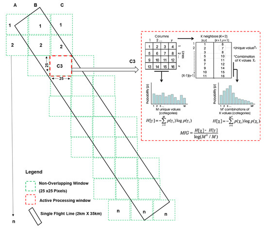
Figure 3.
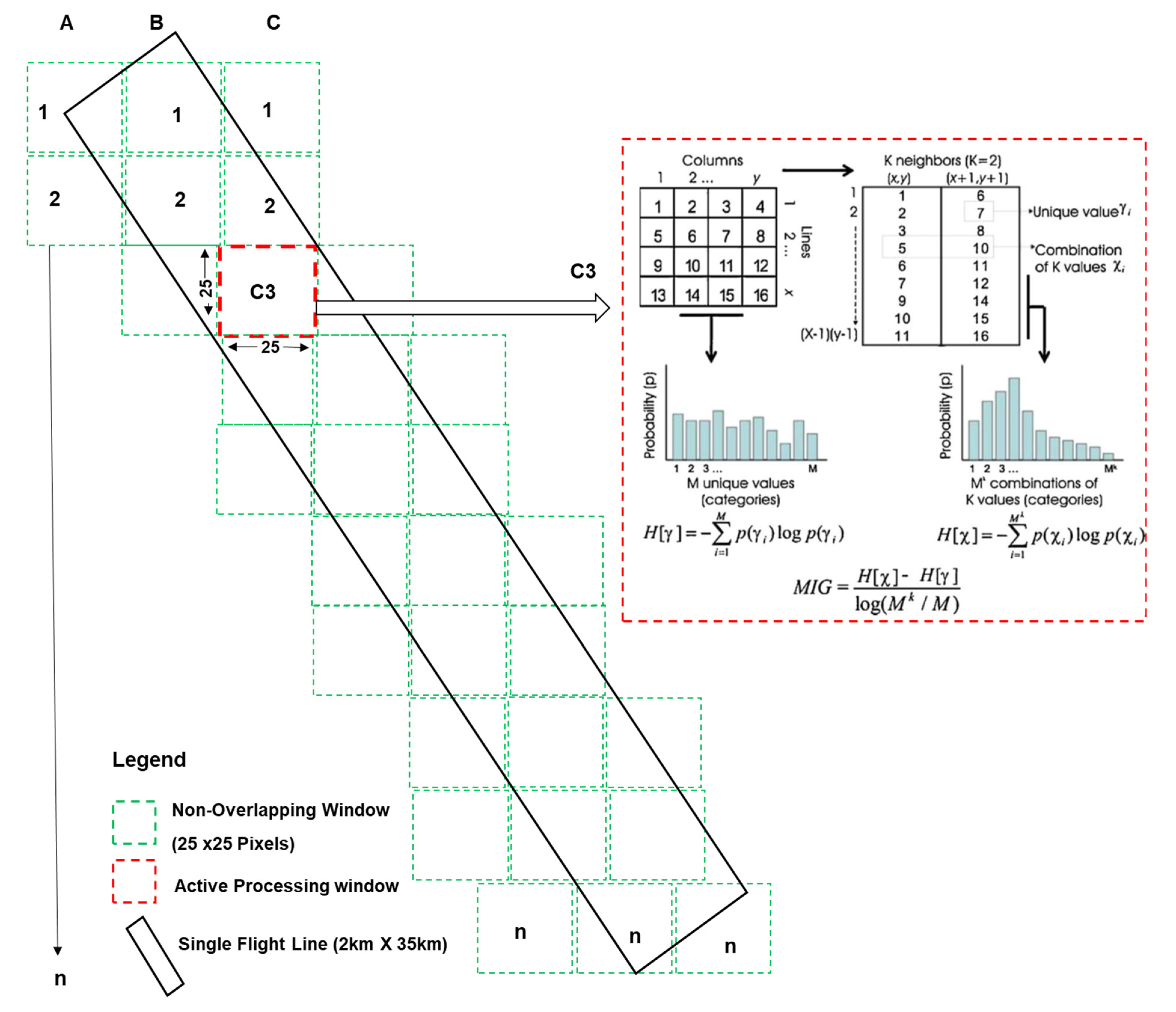
Schematic diagram showing the non-overlapping window approach adopted in the implementation of spectral complexity metrics on hyperspectral imagery. The non-overlapping window outlines are not drawn to scale. Red dashed lines show an active processing window with a diagram showing an example of the MIG (k = 2) computation reprinted from Ecological Indicators, 9/1248–1256, Raphaël Proulx, Lael Parrott, Structural complexity in digital images as an ecological indicator for monitoring forest dynamics across scale, space and time, page 1251, Copyright (2009), with permission from Elsevier.
Spectral Complexity Metrics (SCM)
The SCM were computed in MATLAB v2018b for each spectral band of the CASI (VNIR = 174 bands) and SASI (SWIR = 65 bands) imagery. The methods proposed by [30,32] were followed to compute MIG and ME as described below.
The MIG (Equation (1)) computes the spectro-spatial heterogeneity (p(Xi)) for a given image that is exclusive of the portion of aspatial spectral heterogeneity (p(Yi)) [32].
where:
- k = 4 (i.e., the observed 2 × 2-pixel neighborhood; when k = 4, it means the combination of positions (x, y), (x + 1, y), (x, y + 1) and (x + 1, y + 1) in the image);
- Nk signifies the maximum number of possible reflectance combinations, given a set number of reflectance values (bins), N;
- log (Nk⁄N) is used to normalize MIG values between 0 and 1;
- p(Xi) is the probability of locating a specific 2 × 2 combination of pixel reflectance; and
- p(Yi) is the relative frequency or probability of locating reflectance value (Yi) in the image irrespective of its location.
To avoid biasing due to undersampling of the 2 × 2 reflectance combination in the image, it is generally recommended that the ratio of the total number of pixels in the image to Nk should be greater than 100. Based on this, we chose a bin value (classes of reflectance values), N = 18. We chose the highest theoretically feasible 2 × 2 reflectance combination to preserve as much information as possible [32].
The ME was computed according to Equation (2):
where p(Yi) is the probability of locating a specific pixel reflectance value in a 2-dimensional image independent of the position of that pixel in the image.
The MIG and ME values ranges from 0 to 1 with the 0 corresponding to patterns with uniform spectral composition whilst high values close to 1 depict random or highly differentiable patterns (Figure 4).
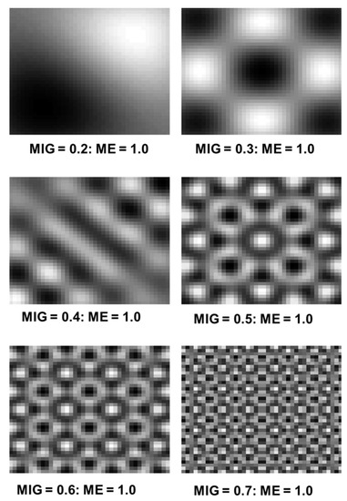
Figure 4.
Comparison of changing MIG (0.2–0.7) with a constant ME. Reprinted from Ecological Indicators, 8/270–84, Raphaël Proulx, Lael Parrott, ‘Measures of structural complexity in digital images for monitoring the ecological signature of an old-growth forest ecosystem’, page 15, Copyright (2008), with permission from Elsevier.
2.5. Mangrove-Forest Classification
A forward feature selection (FFS) [50] was implemented on all three versions of the data (i.e., spectral reflectance, ME, and MIG) with the PRTools toolbox version 5.4.2 [51,52] in Matlab v2018b to reduce the dimensions of the data while identifying the optimal bands that best separates the classes. For the mangrove extent classification, 500 pixels of SCM and 6000 pixels of reflectance at the native spatial resolution (2.5 m) representing both terrestrial forest and mangroves were selected from one of the flight lines. We then implemented the FFS on these data based using the nearest neighbor (NN) criterion. The FFS algorithm selects the features (i.e., bands) by first identifying the most distinct, sequentially adding bands to the set in the order that they improve the separability of the classes [50].
Theoretically, to avoid overfitting, the maximum number of bands (F) necessary for separation of the number of classes can be determined from Equation (3) [53].
where n is the number of samples and g is the number of classes.
Next, we extracted the optimal bands from the FFS to train and evaluate the classification performance of selected machine learning (ML) algorithms in MATLAB R2018b. Four ML classifiers frequently used in the literature, namely, k-nearest neighbor (KNN), quadratic support vector machine (Q-SVM), linear and quadratic discriminant (LDA and QDA) classifiers were tested. The classification performance of each ML algorithm was assessed using a 20% hold-out equivalent to minimum of 50 samples per class (i.e., using 80% of the dataset for training and 20% for testing).
2.6. Mangrove Species Classification
We used ArcGIS 10.7.1 to georeference published ground data of mangrove species distribution over the study area [41]. This reference map from [43] was produced using a combination of aerial photographs, Quickbird satellite imagery, and 1127 sample points from 77 field plots (60 m × 10 m) distributed across the study area. We overlaid the reference map on the HSI and extracted 181 ground truth regions of interest randomly distributed across the study area (Figure S1). Each region covered approximately 1.6 ha and represented the six predominant classes (five mangrove species classes and a forest class). The mangrove species classes included 3 pure stands: Acrostichum aureum (ACAU), Pelliciera rhizophorae (PERH), Rhizophora racemosa (RHRA); two mixed stands: Acrostichum aureum–Rhizophora racemosa (ACAU–RHRA), Rhizophora racemosa–Pelliciera rhizophorae (RHRA–PERH); and a forest class. To compare the separability of these predominant mangrove species, the spectral reflectance data were re-sampled to the same spatial resolution as the SCM (nearest neighbor resampling). Next, an FFS was run separately on the reflectance data (both native resolution and spatially resampled) and the SCM using pixels within the ground truth target areas. Table 3 provides a summary of the number of training pixels used for the analysis per metric. We increased the total sample size to 30,000 pixels to constitute 5000 pixels per class to capture spectral variability of the reflectance for classification, due to the small pixel size of the reflectance data at the native spatial resolution.
Table 3.
Total number of training pixels used for FFS and classification for each metric at different spatial resolutions.
Using the optimal bands selected from the FFS, we trained KMM, LDA, and Q-SVM classifiers in MATLAB v2018b.
Next, the accuracy of each classifier was assessed using a confusion matrix. The sample size (i.e., >150 pixels) used for the calculation of the error matrix was consistent with the minimum sample requirement, as determined using a multinomial distribution equation [54]. For the six predominant species classes (k = 6) and a desired confidence level (α) of 90%, the minimum sample size can be calculated (Equation (4)):
where:
- B = Upper (α/k) × 100th percentile determined from an χ2 distribution table with 1 degree of freedom
- = Proportion of area occupied by class (i)
- bi = precision for each class (i.e., 0.1)
2.7. Computation of Spectral Beta (β) Diversity
Finally, to determine the spectral variability of the predominant mangrove species, we calculated a measure of spectral β diversity for each mangrove class. For the reflectance data (2.5 m) from within each of the ground truth regions of interest for each class, 500 randomly sampled pixels were used (n = 83,500). For the SCM (25 m) and spatially resampled reflectance, (25 m), approximately 2000 pixels representing all 6 classes were used for the computation of β diversity. The spectral β diversity is a measure of the spectral variation of each mangrove class. Following [55], we calculated the spectral β diversity of the predominant mangrove species classes using MIG and ME at a spatial resolution of 25 m, and spectral reflectance at both 2.5 and 25 m. For the sum-of-squares partitioning approach to calculating the spectral β diversity it is imperative that all communities (regions of interest: ROI) have an equal number of pixels [55]. To achieve this, we sampled a constant (m) number of pixels in each ROI selected for each input data (i.e., SCM and reflectance). By extracting the mean of the (m) pixels in each ROI (k) and grouping per class, we computed β diversity (SSβ,k) using Equations (5) and (6).
where:
- Skj = Squared deviation of the kth community (ROI) and jth band.
- ŷkj = The mean of m pixels of ROI (k) per class corresponding to the jth band.
- ŷj = The mean of each class (column) and corresponding to the jth band.
A Shapiro–Wilk test of normality was conducted for SSβ,k of all classes. Based on the outcome of the normality test, either a Tukey post-hoc test or Kruskal–Wallis test was implemented to examine the differences in spectral variability between each pair of the mangrove species at a 95% confidence level.
3. Results
3.1. Spectral Consistency
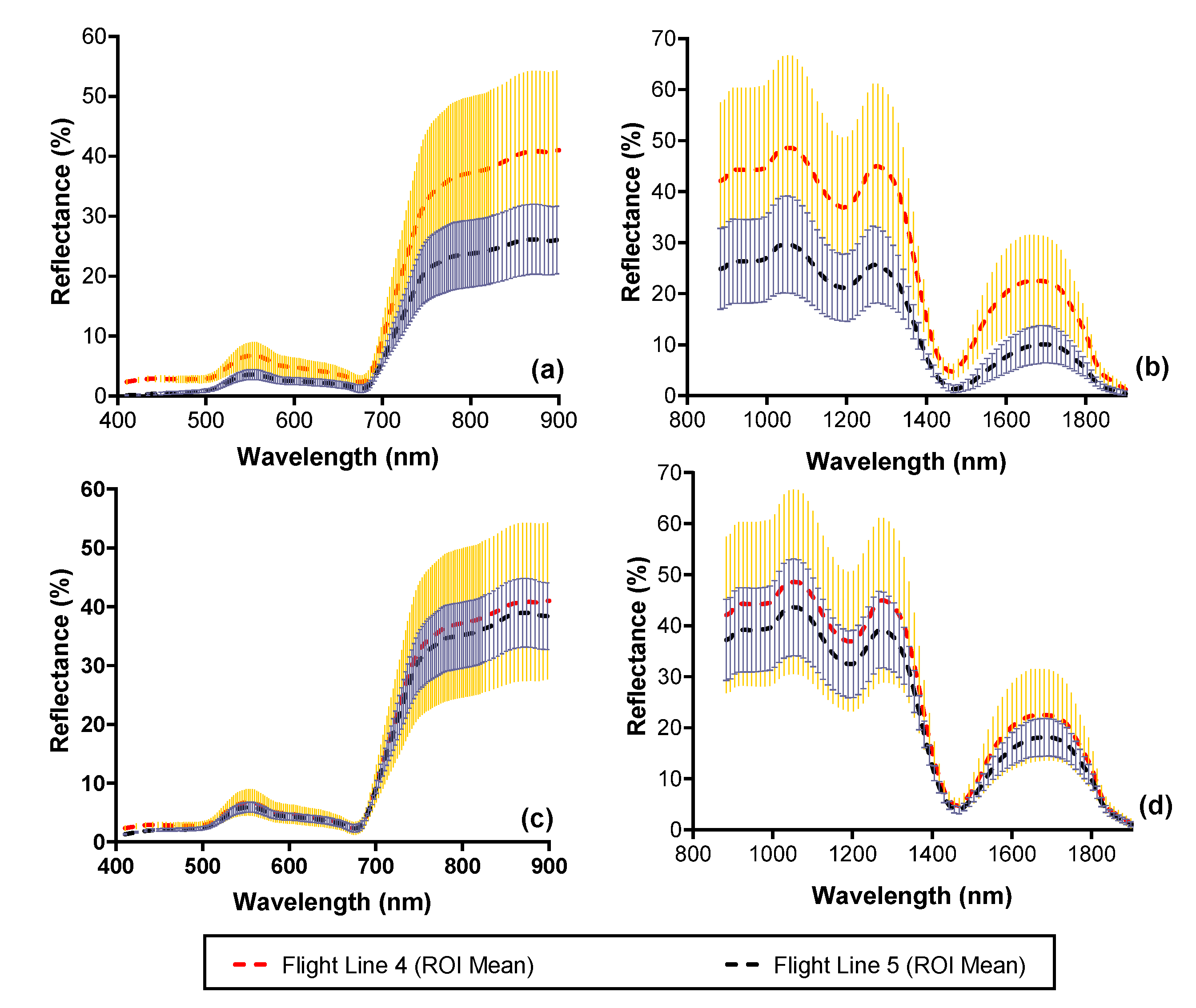
An example of the mean and standard deviation of vegetation spectra representing the same mangrove vegetation covering 41.8 ha (~67,000 pixels) from two neighboring flight lines before and after illumination normalization is shown in Figure 5. Prior to the illumination normalization, the spectra were quite dissimilar with differences of up to 30% for the VNIR and up to 20% for the SWIR. After normalization, the spectral similarity improved with differences < 5% across the spectral range indicating an improvement in the spectral consistency (Figure 5c,d) across the two flight lines.
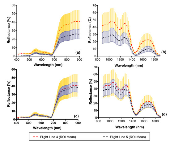
Figure 5.
Mean and standard deviation of reflectance of mangrove vegetation covering 41.8 ha (67,000 pixels) from the CASI and SASI imagery before (black dashed line) and after (red dashed line) applying the BRDF correction. Plots a and b show the difference in reflectance spectra before correction for the CASI (a) and SASI (b). Plots c and d show the reflectance spectra for the CASI (c) and SASI (d) after correction. Error bars illustrate one standard deviation.
3.2. Spectral Reflectance and Spectral Complexity Metrics
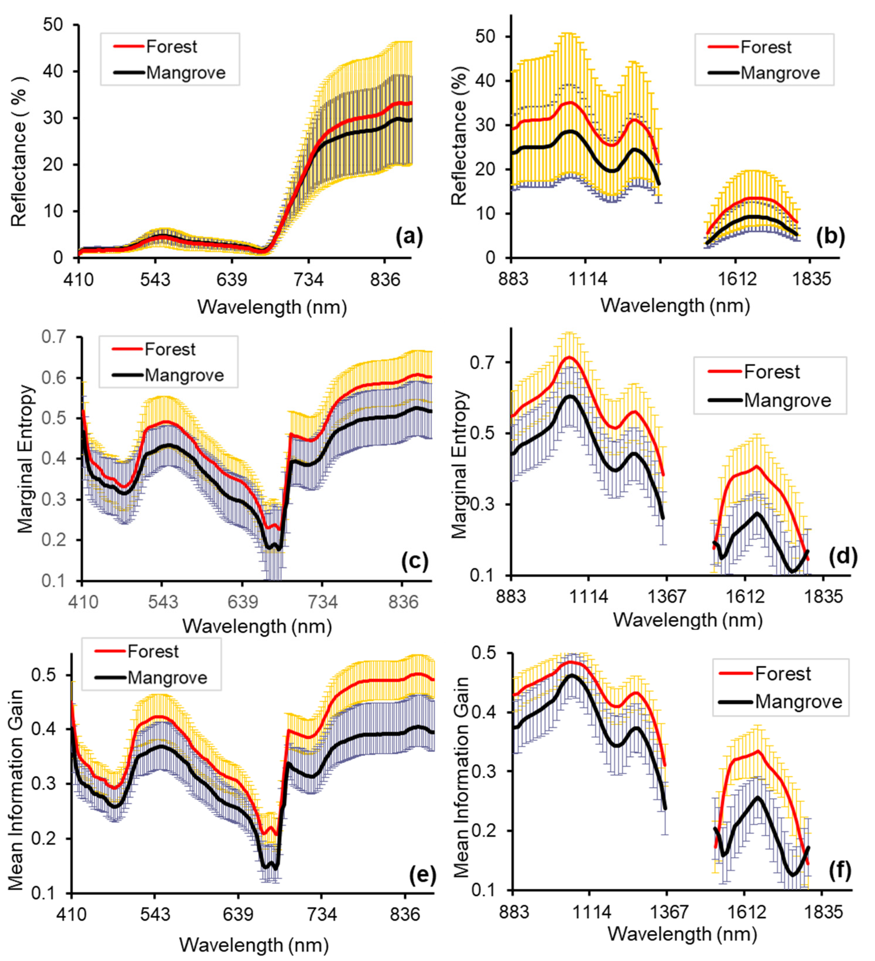
The mean and standard deviation of the spectral reflectance, ME, and MIG representing forest and mangrove, are shown in Figure 6. For the reflectance data, across the blue through red-edge wavelength range, the mean spectra of mangrove and forest are very similar (<1% difference). The difference increased to 1–4% difference in the NIR and up to 7% in the SWIR (Figure 6).
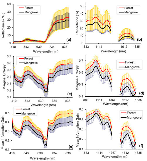
Figure 6.
Comparison of mangrove and forest reflectance (%) (mean and standard deviation of 250 pixels), Marginal Entropy (ME), and Mean Information Gain (MIG): (a) spectral reflectance in the VNIR (2.5 m); (b) spectral reflectance in the SWIR (2.5 m); (c) ME -VNIR (250 m); (d) ME -SWIR (62.5 m); (e) MIG -VNIR (250 m); (f) MIG-SWIR (62.5 m). Scales with the best separability between forest and mangrove for the SCM are shown (see Section 3.3). The MIG and ME values of forest were larger than that of mangrove from the VNIR to the SWIR region of the electromagnetic spectrum except at 1516 nm and 1792 nm. In the VNIR portion of the spectrum, the difference between forest and mangrove ranged between 0.03–0.1 for MIG and 0.02–0.08 for ME. In the SWIR portion of the electromagnetic spectrum, the difference between forest and mangrove ranged between 0.01 to 0.13 for MIG and 0.02–0.18 for ME. The greatest differences between both mean MIG and ME of forest and mangrove were recorded in the NIR (>765 nm) and between the wavelength ranges 1553 nm–1738 nm for SWIR (Figure 6).
3.3. Mangrove Extent Classification
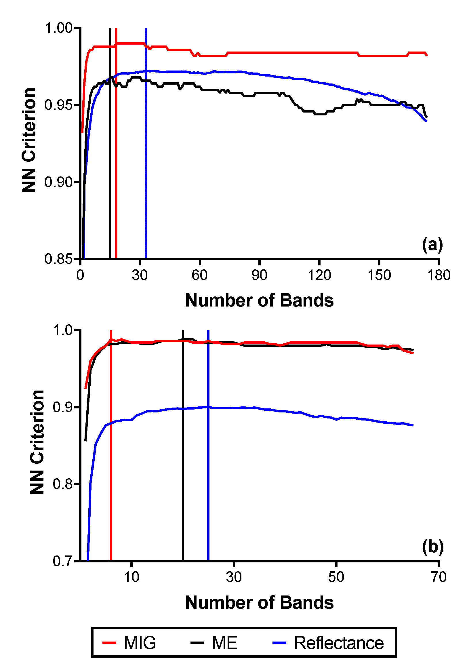
The summaries of the results for the FFS (reflectance and SCM) are presented in Figure 7 and Figure S2. With the reflectance data at the native spatial resolution, 33 bands were optimal in the VNIR, corresponding to a separability value of 0.97, while 26 bands were optimal (separability value = 0.90) in the SWIR. Figure 8 shows the respective positions of the optimal bands in the electromagnetic spectrum for both VNIR and SWIR reflectance (2.5 m). After the transformation of VNIR reflectance to the SCM, the best separability was achieved with a window size of 250 m (100 × 100 pixels). The optimal bands reduced to 18 for MIG, and 15 for ME, with separability values of 0.99 and 0.97, respectively (Figure 9a). For the SCM–SWIR, the best separability was achieved at the 62.5 m scale (Figure 7 and Figure S2). Six bands were optimal for MIG–SWIR with a separability value of 0.99, while 20 optimal bands corresponding to a separability value of 0.99 were selected for ME–SWIR. The position of the optimal spectral bands for MIG–SWIR is shown in Figure 9b. Figure S2 presents the results for the FFS from the other windows sizes.
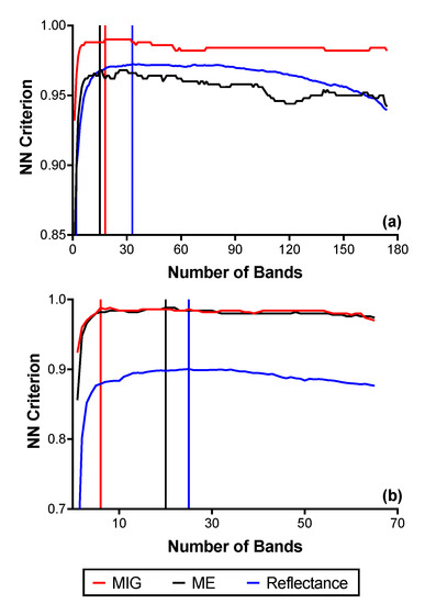
Figure 7.
Results from the forward feature selection (FFS) implemented on reflectance and SCM data with the highest NN criterion values: (a) VNIR reflectance (2.5 m), MIG–VNIR (250 m), and ME–VNIR (250 m); (b) SWIR reflectance (2.5 m), MIG–SWIR (62.5 m), and ME–SWIR (62.5 m).
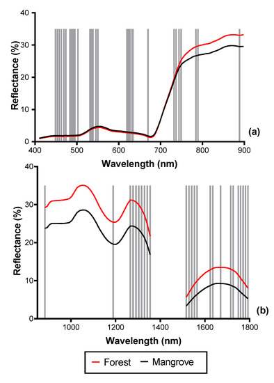
Figure 8.
Spectral reflectance of mangrove and terrestrial forest with vertical lines showing the positions of the optimal bands selected by the forward feature selection (FFS). (a) 33 bands selected from the VNIR reflectance (2.5 m), (b) 26 bands selected from the SWIR reflectance (2.5 m) data.
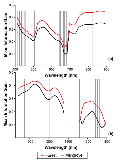
Figure 9.
SCM of mangrove and terrestrial forest with vertical lines showing the positions of the optimal bands selected by the forward feature selection (FFS). (a) Eighteen bands selected from the MIG–VNIR (250 m), (b) 6 bands selected from the MIG–SWIR (250 m) data. Because separability was higher for MIG, positions of optimal ME bands not shown.
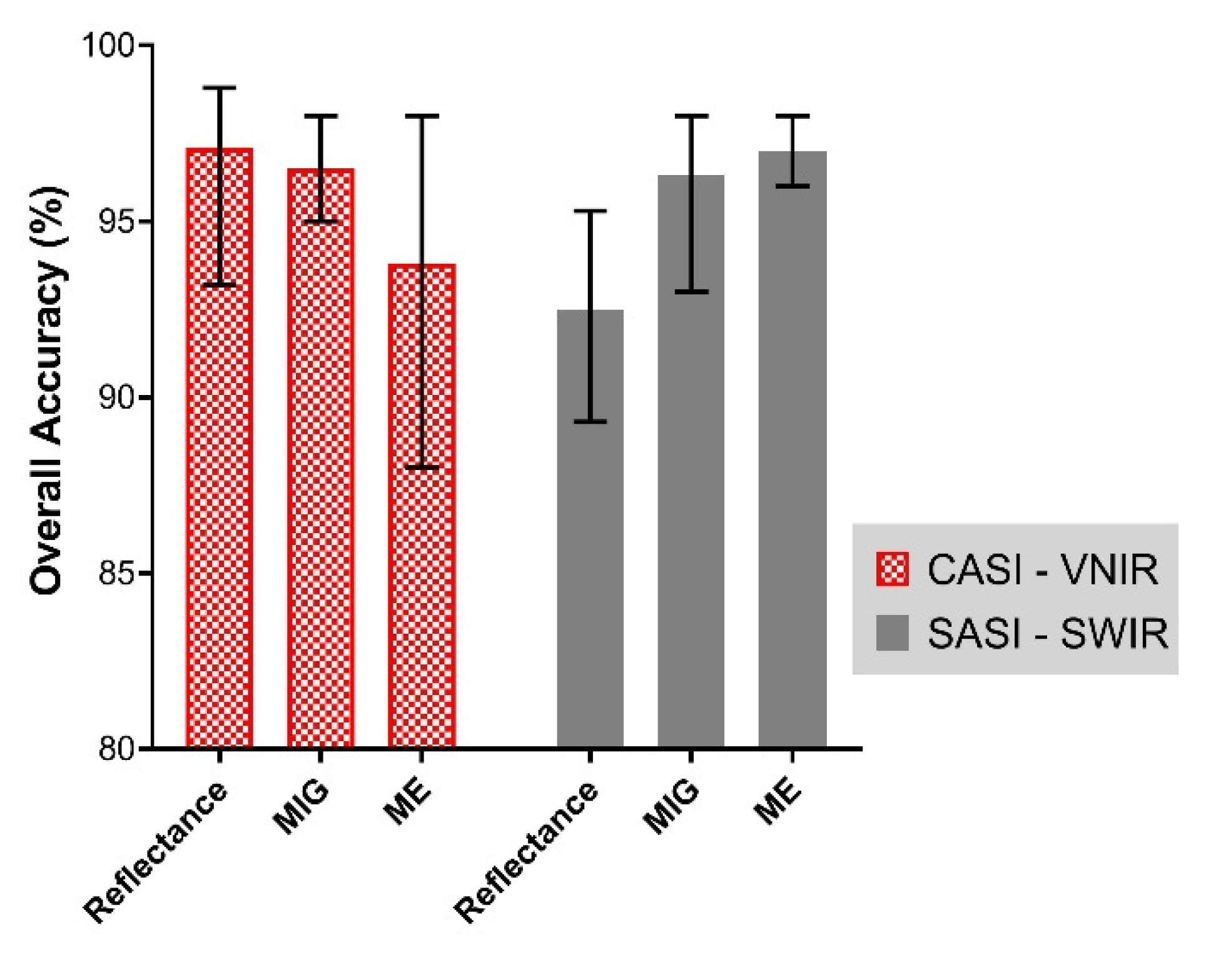
The overall best mangrove extent classification accuracy using the optimal bands (Figure 7, Figure 8 and Figure 9) is shown in Figure 10. The overall best mangrove classification accuracy attainable with the reflectance data at the native spatial resolution was 98.8% and 95.3% for CASI (VNIR) and SASI (SWIR), respectively (Q-SVM classifier). However, the SCM–SWIR (both MIG and ME) had a classification accuracy 2.7% higher than reflectance (i.e., 98%) (Figure 10) for both MIG (KNN classifier) and ME (Q-SVM classifier) The overall best classification accuracy for MIG (VNIR) and ME (VNIR) was 98% (KNN classifier for both).
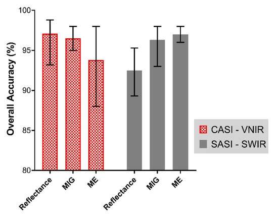
Figure 10.
The mean classification accuracy for mangrove and forest achieved for each of the input datasets assessed in this study (i.e., Reflectance, MIG, and ME) for both VNIR and SWIR imagery. The error bars illustrate the minimum and maximum overall classification accuracy achieved for each dataset.
The overall classification performance was comparable for reflectance (VNIR) and SCM (VNIR). However, with the SCM (SWIR) data, the overall classification was more accurate compared to reflectance (SWIR). The summary of classification performance of the different metrics is presented in Figure 10.
3.4. Feature Selection for Species Discrimination
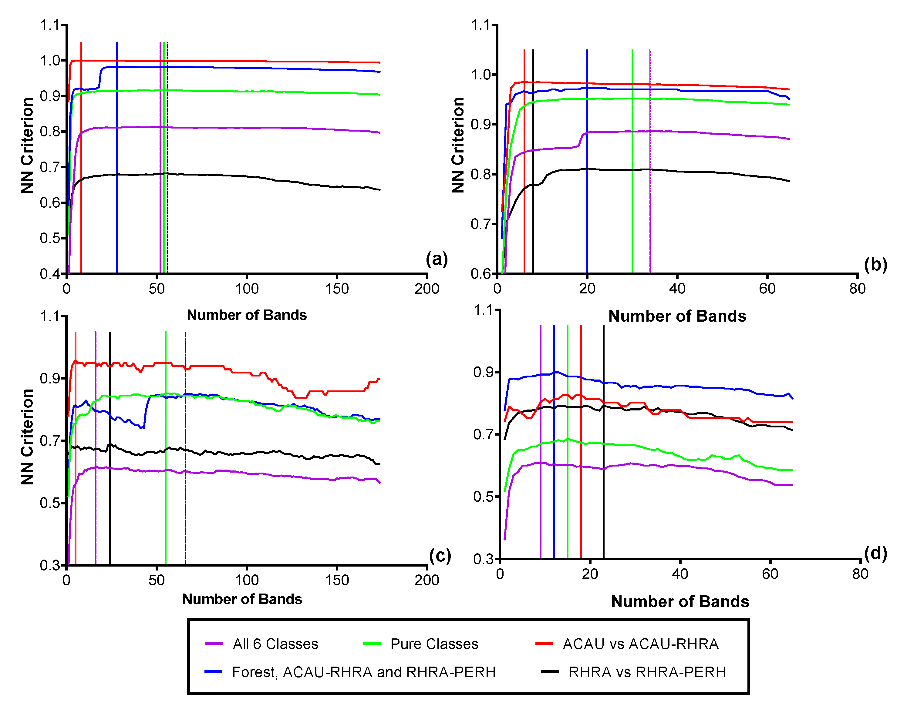
Based on the FFS at the native spatial resolution of 2.5 m, for the spectral reflectance, 52 optimal bands (VNIR) were needed to separate the six classes resulting in a nearest-neighbor (NN) criterion value of 0.81 (Figure 11a). For the SWIR reflectance data at 2.5 m, 34 bands were optimal (NN Criterion = 0.89) for the six classes (Figure 11b). This shows a better separability in the SWIR between the six predominant species classes compared to VNIR reflectance. It is important to note that due to the small pixel size of the imagery, different sets of randomly selected representative pixels will result in different sets of optimal bands. At the coarsest SCM scale (62.5 m), a maximum criterion value of 0.92 (38 optimal bands) was achieved for MIG–VNIR (Figure 12), while for ME–VNIR, 30 bands were optimal with a criterion value of 0.90. For MIG–SWIR, (62.5 m), 26 optimal bands achieved the highest overall separability value of 0.85. For ME (62.5 m), 21 optimal bands resulted in a separability of 0.81.

Figure 11.
Optimal bands from the FFS for discriminating the six predominant species classes from (a) VNIR reflectance (2.5 m), (b) SWIR reflectance (2.5 m), (c) VNIR reflectance resampled to the coarsest SCM spatial (62.5 m), (d) SWIR reflectance resampled to the coarsest SCM spatial resolution (62.5 m).
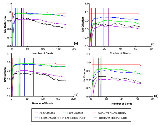
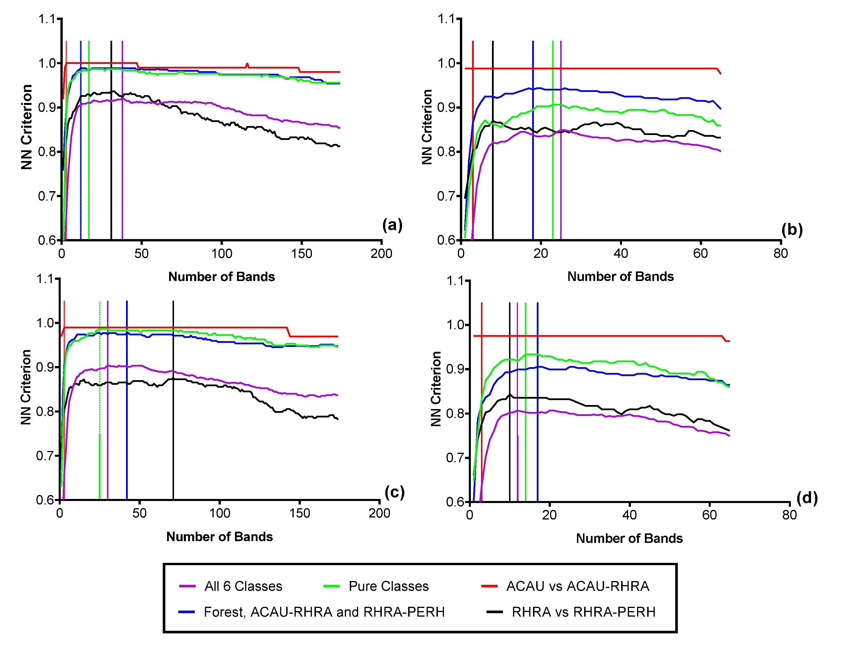
Figure 12.
Results of the forward feature selection to determine the separability and optimal bands necessary for discriminating the six predominant species using SCM at the coarsest scale (62.5 m): (a) MIG–VNIR (b) MIG–SWIR, (c) ME–VNIR and (d) ME–SWIR.
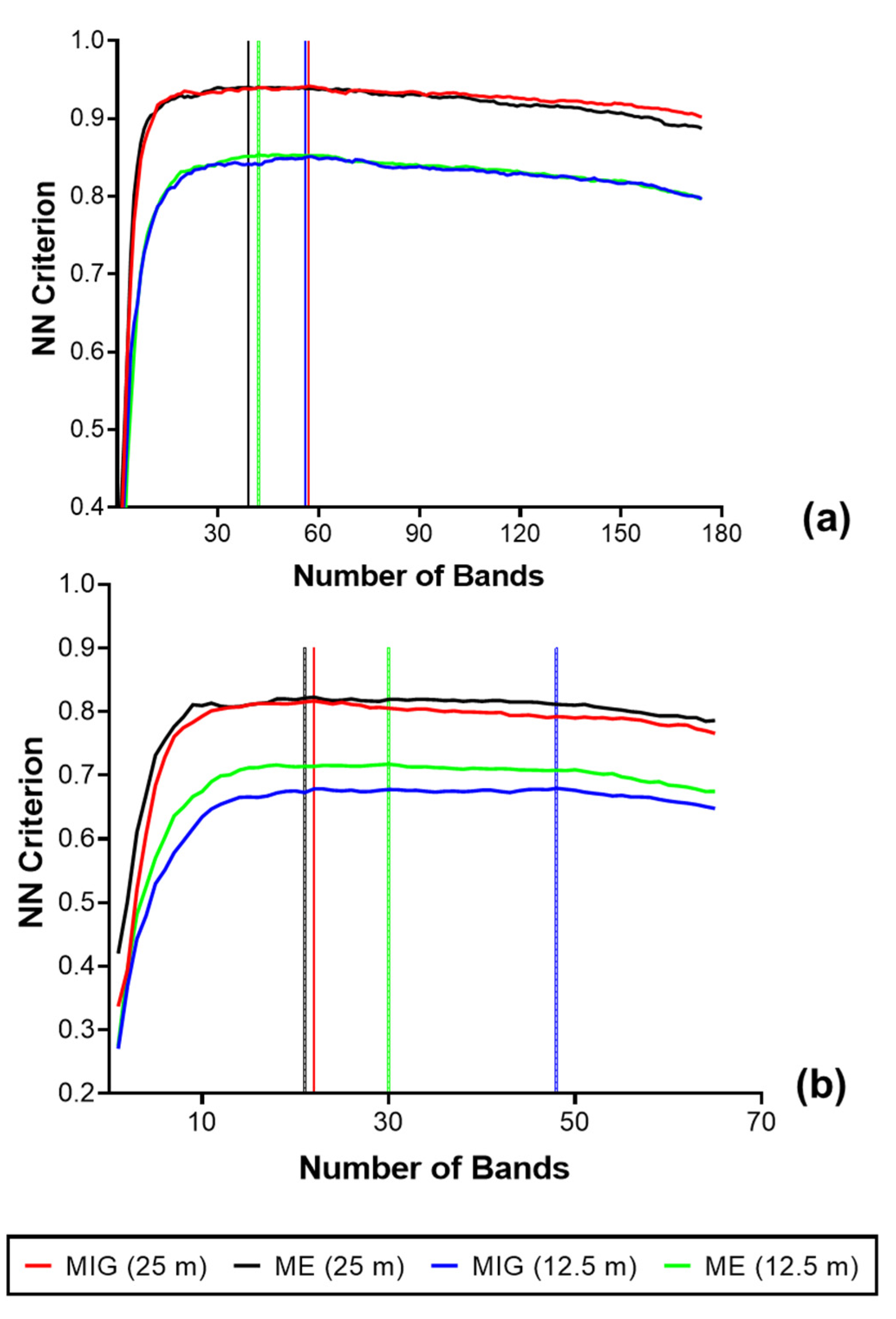
The greatest separability between the species classes was found for an SCM window size of 25 m with 0.94 for both ME–VNIR (39 optimal bands) and MIG–VNIR (57 optimal bands) (Figure 13). At the smallest SCM window size of 12.5 m, the separability of the six classes was the lowest at 0.85 for both ME–VNIR and MIG–VNIR. For SCM–SWIR, a separability of 0.82 was recorded for both ME and MIG (25 m spatial resolution). The lowest separability was recorded for the SWIR at the 12.5 m resolution: 0.68 for MIG and 0.72 for ME.
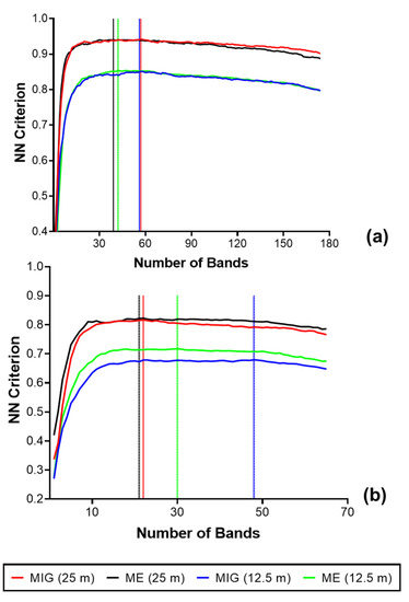
Figure 13.
Results of the FFS to determine the separability and optimal bands necessary for discriminating predominant species and forest class using SCM computed at 12.5 and 25 m: (a) VNIR (b) SWIR.
Additionally, the results of the FFS for only the pure classes made up of PERH, ACAU, and RHRA show that at 2.5 m, 54 bands in the VNIR and 30 bands in the SWIR reflectance could attain a high NN criterion of 0.92 and 0.95, respectively. With 22 optimal bands, MIG–VNIR (25 m) and ME–VNIR (25 m) recorded criterion values of 1 to constitute the best separability for the pure classes. In contrast, the SCM–VNIR recorded a criterion value of 0.987 (17 optimal bands) for MIG and 0.987 (25 optimal bands) for ME at the coarsest scale (62.5 m). The outcome of the FFS also shows SCM–VNIR (25 m) having better separate specific class combinations (such as ACAU–RHRA versus RHRA–PERH) than the reflectance at native resolution. The results further show that the NN criterion values of all the metrics were highest for ACAU versus ACAU–RHRA ranging between 0.976–1. This indicates a greater separability of the ACAU and ACAU–RHRA class pair compared to the other classes examined in this study.
3.5. Species Classification
Figure 14 shows a comparison of the classification accuracies attained when the window size is varied from 12.5 to 62.5 m. For the VNIR, the lowest classification error was achieved with ME (93.6%, Q-SVM classifier) at a window size of 25 m. In comparison, the highest classification accuracy from the reflectance at the native spatial resolution was 89.7% (Q-SVM classifier). The best classification accuracy for the SWIR was achieved by ME (84.5%, Q-SVM classifier, 25 m). However, the best SWIR classification was found for reflectance at the native spatial resolution (2.5 m) resulting in an accuracy of 94.8% with the Q-SVM classifier (Figure 14).
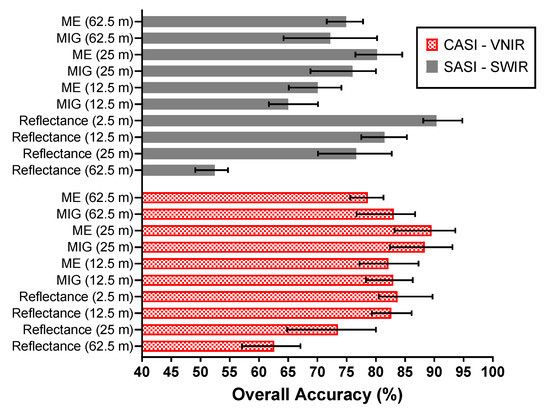
Figure 14.
A comparison of the mean classification accuracies for different window sizes 62.5 m, 25 m, and 12.5 m of reflectance data and SCM. The error bars illustrate the minimum and maximum overall classification accuracy achieved for each dataset.
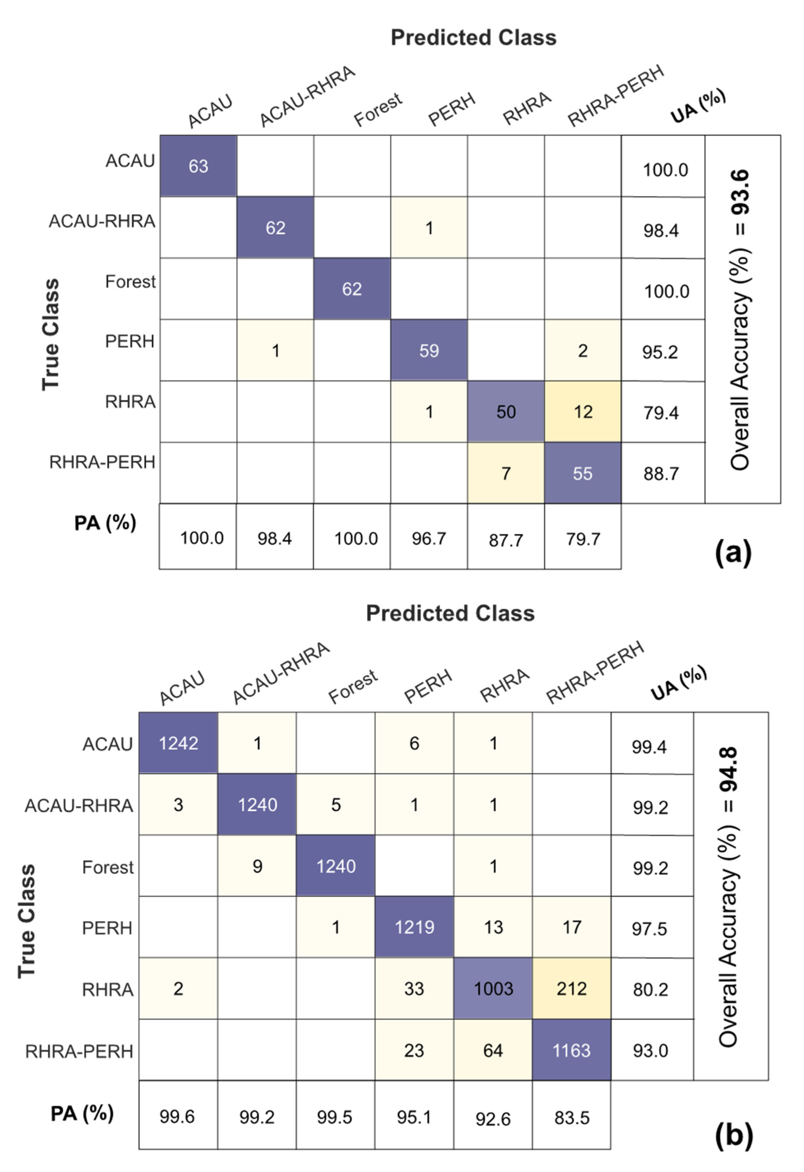
The overall best SCM–VNIR classification performance was found with the 25 m (10 × 10 pixel window) 93.1% and 93.6% for MIG and ME, respectively, in comparison to 80% for 25 m spatially resampled VNIR reflectance (Figure 14). At 25 m, SCM–SWIR recorded a classification accuracy between 68.8–83.7% comparable to what was recorded for SWIR reflectance (25 m) in the range of 70.1–82.7%. Figure 15 illustrates the confusion matrix of the best performing classifiers ME–VNIR at 25 m spatial resolution (Q-SVM classifier) and 2.5 m SWIR reflectance (Q-SVM classifier). The producer’s accuracy for ME–VNIR ranged between 79.7–100% whilst the user’s accuracy ranged between 79.4–100% (Figure 15a). The producer’s accuracy for SWIR 2.5 m reflectance ranged from 83.5% to 99.6% and the user’s accuracy ranged from 80.2% to 99.4% (Figure 15b). The best classification outcome for SCM–SWIR was achieved by ME (25 m) with an accuracy of 84.5%. Further evaluation of the confusion matrix of the best VNIR classifier revealed that most of the confusion was between the RHRA and RHRA–PERH classes. For the best SWIR classifier (Figure 15b), the majority of the confusion was between PERH, RHRA, and RHRA–PERH. The confusion matrices for the other classifiers and scales are presented in Figures S3–S11. A species distribution map using ME–VNIR data (25 m) with the Q-SVM classifier is shown in Figure 16.
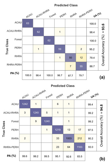
Figure 15.
Confusion matrices for the best VNIR and SWIR classifications: (a) ME–VNIR (25 m) with the Q-SVM classifier; (b) SWIR reflectance (2.5 m) with the Q-SVM classifier. PA = Producer’s Accuracy; UA = User’s Accuracy.

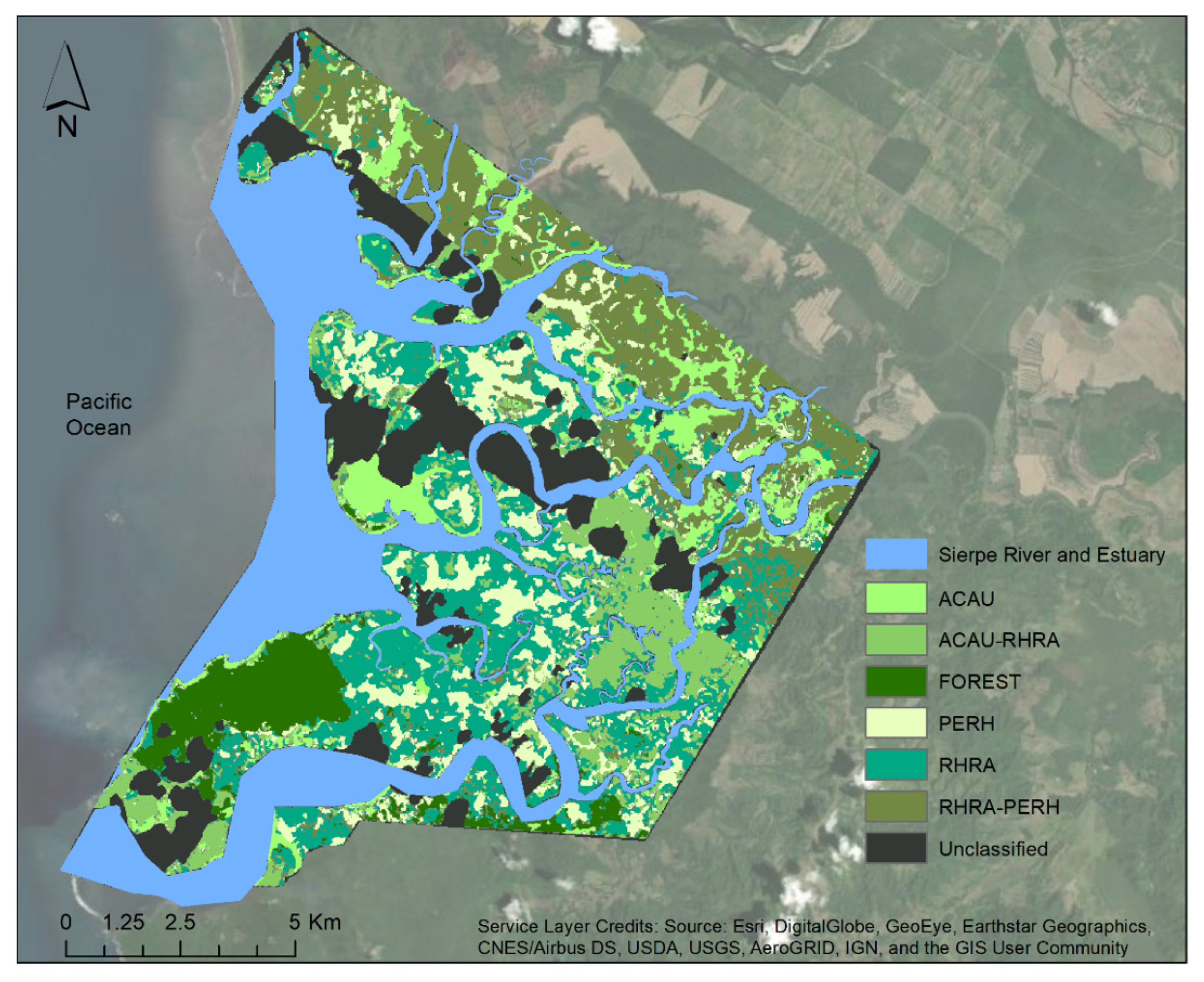
Figure 16.
Species distribution map of Terraba Sierpe Mangroves produced from VNIR–ME (25 m window size) as input for a Q-SVM classifier. The unclassified areas are the pixels with clouds and cloud shadows.
3.6. Spectral Beta (β) Diversity
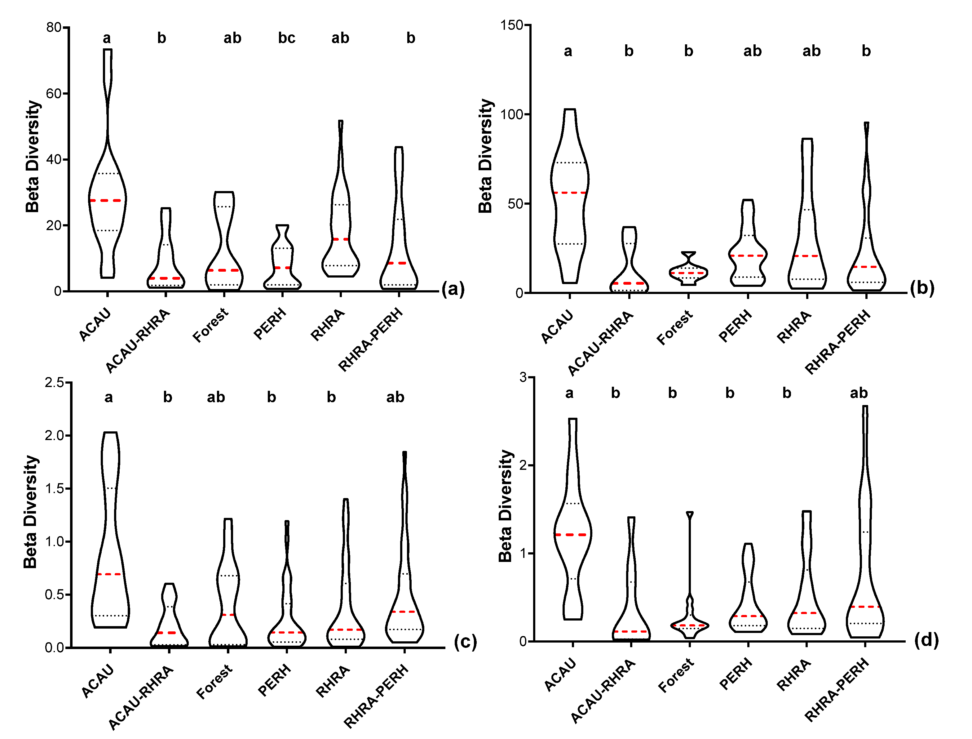
For reflectance data (VNIR) at the native pixel size of 2.5 m, the spectral β diversity was highest for ACAU (µ = 29.51 ± 18.13) and lowest for PERH (µ = 8.1 ± 6.3) (Figure 17a). Similarly, ACAU and the forest class recorded the highest (µ = 52.4 ± 27.22) and lowest (µ = 11.88 ± 5.4) spectral variability, respectively, in the SWIR reflectance (Figure 17b). The spectral β diversity of the reflectance data (both VNIR and SWIR) at 2.5 m did not always follow a normal distribution; the post-hoc Kruskal–Wallis test showed significant differences (p < 0.05) between ACAU versus forest, ACAU–RHRA and RHRA–PERH. In addition, a significant difference (p < 0.05) was observed between PERH and RHRA for the VNIR reflectance. After resampling the reflectance data to the same spatial scale as the SCM (25 m), the overall values of β diversity decreased. At the 25 m pixel size, in the VNIR, β diversity was highest for ACAU (µ = 0.87 ± 0.64) and lowest for ACAU–RHRA (µ = 0.21 ± 0.20) (Figure 17c). For the SWIR (25 m), RHRA–PERH and forest recorded the highest (µ = 0.77 ± 0.75) and the lowest spectral β diversity (µ = 0.29 ± 0.35) (Figure 17d). Significant differences (p < 0.05) were observed between ACAU and other classes except RHRA–PERH for SWIR reflectance (25 m) while the differences between ACAU versus PERH, RHRA, and ACAU–RHRA were significant for VNIR spatially resampled reflectance (25 m).
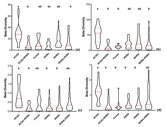
Figure 17.
Violin plots showing the 10th and 90th percentiles range of spectral β diversity for five predominant mangrove species (ACAU, ACAU–RHRA, PERH, RHRA, and RHRA–PERH) and a forest class for (a) VNIR spectral reflectance at the 2.5 m native spatial resolution. (b) SWIR spectral reflectance at the 2.5 m native spatial resolution, (c) VNIR spectral reflectance resampled to the same spatial resolution (25 m) as MIG/ME, (d) SWIR spectral reflectance resampled to the same spatial resolution (25 m) as MIG/ME. Red dashed lines represent median and the dotted lines represent the quartiles. Different superscripts letter indicates statistically significant (p < 0.05) differences between pairs of predominant mangrove species classes.
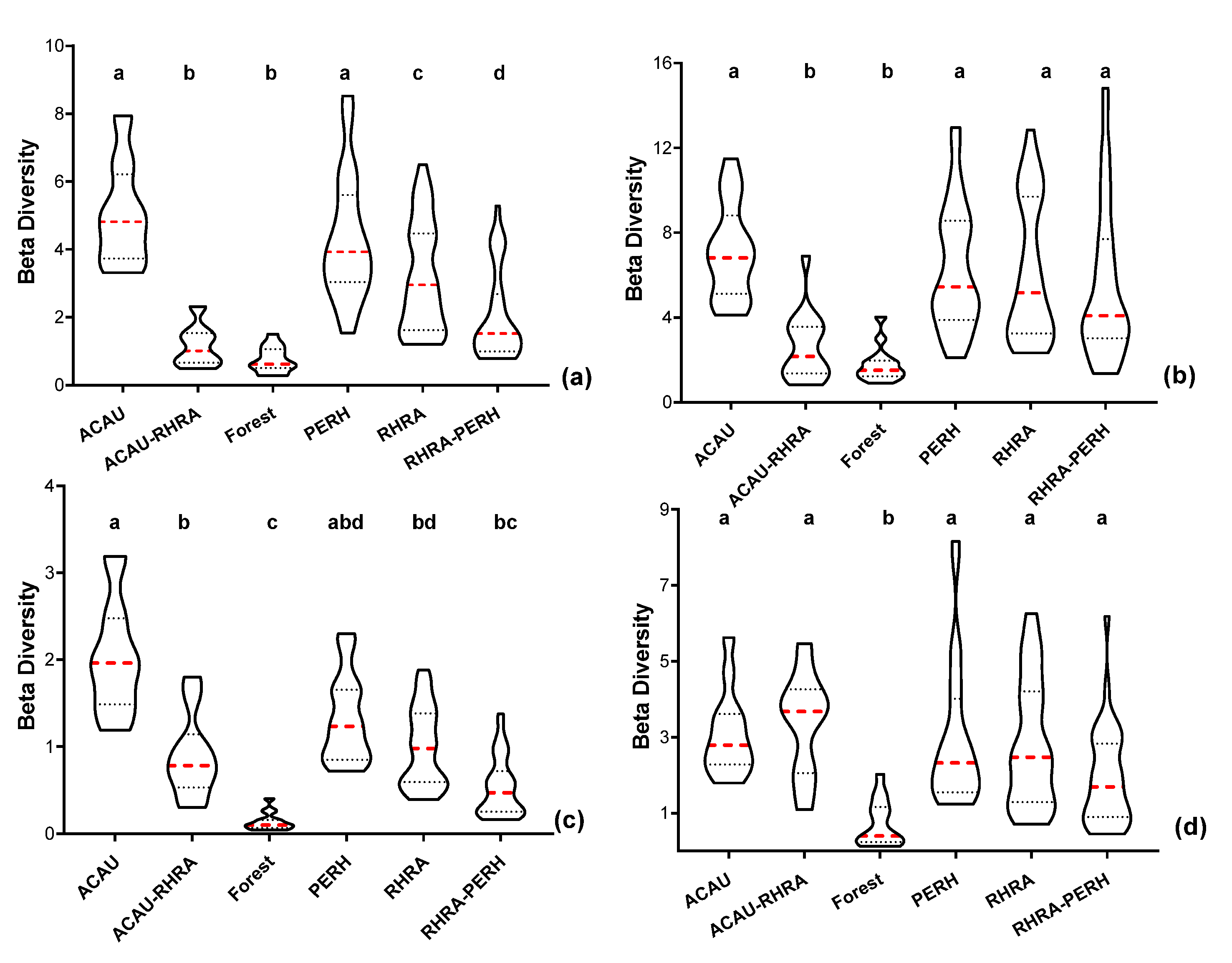
For MIG–VNIR (25 m), the variation in spectral β diversity was highest for the PERH class (µ = 4.3 ± 1.83) with the least variability recorded by forest class (µ = 0.75 ± 0.38) (Figure 18a). Additionally, for ME–VNIR, RHRA–PERH had the highest variation in spectral β diversity (µ = 5.5 ± 3.6), while the lowest was attained by the forest class (µ = 1.8 ± 0.84) (Figure 18b). Statistically significant differences (p < 0.05) were found between the forest and ACAU–RHRA versus pure species and RHRA–PERH for ME–VNIR. Additionally, for the MIG–VNIR, except for ACAU–RHRA versus forest and RHRA–PERH as well as ACAU versus PERH, significant differences (p < 0.05) were also found between a pair of the remaining classes. Considering SCM in the SWIR (25 m), MIG spectral β diversity was highest for the ACAU class (µ = 2.0 ± 0.65), while forest recorded the lowest values diversity (µ = 0.14 ± 0.10). For MIG–SWIR (25 m), the differences between the forest class and all other classes except RHRA–PERH were statistically significant (p < 0.05) (Figure 18c). In addition, the difference between ACAU versus RHRA and RHRA–PERH was also statistically different for MIG–SWIR (25 m). With regards to ME–SWIR, PERH is considered to have the highest β diversity (µ = 3.0 ± 1.9), while the forest class had the lowest β diversity (µ = 0.72 ± 0.61) (Figure 18d). The results for the post-hoc multiple comparison test for ME–SWIR (25 m) indicates that there were statistically significant differences between the forest and all other classes.
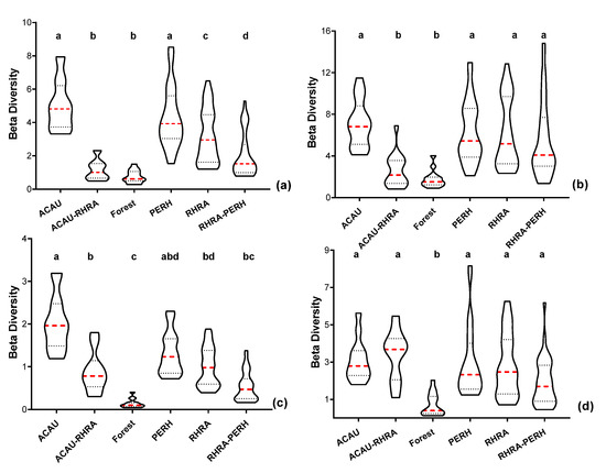
Figure 18.
Violin plots showing the 10th and 90th percentiles range of spectral β diversity computed from the SCM at 25 m spatial resolution. Each box represents one of the five predominant mangrove species classes (ACAU, ACAU–RHRA, PERH, RHRA, and RHRA–PERH) and a forest class. (a) MIG–VNIR, (b) ME–VNIR, (c) MIG–SWIR, and (d) ME–SWIR. Red dashed lines represent median and the dotted lines represent the quartiles. Different superscripts letter indicates statistically significant (p < 0.05) differences between pairs of predominant mangrove species classes.
4. Discussion
The results from our study represent the first attempt to classify mangrove extent and mangrove species using SCM: MIG (spectral reflectance spatial heterogeneity) and ME (spectral reflectance aspatial heterogeneity) derived from airborne HSI. While the highest accuracy separating mangroves from terrestrial forest in the VNIR was found for the reflectance data at the native spectral resolution (OA = 98.8%, Figure 10), classification accuracy of both SCM metrics outperformed the original spectral reflectance in the SWIR by 2.7%. In consideration of current and upcoming spaceborne HSI systems with coarser spatial resolutions (e.g., 30 m PRISMA, DESIS, EnMAP, HyspIRI), the classification accuracy from ME–VNIR with a 25 m window size also performed nearly as well (OA = 92%). Although the mean canopy spectral reflectance of forest and mangrove were comparable in the visible spectrum (Figure 6), there were differences in the amplitude in the SCM spectra (Figure 6). The observed differences in MIG and ME values for mangrove and terrestrial vegetation in the visible spectrum can be associated with differing chlorophyll absorption for those vegetation types [56]. Canopy structural differences between mangrove and forest is responsible for observable differences in MIG and ME beyond 680 nm wavelength range [57]. Furthermore, dissimilarity of the reflectance spectra for both classes in the shortwave infrared region can be attributed to differences in water content of the habitats of mangrove and terrestrial forest, with mangrove forest found in substrate with a high water content due to accumulation as a function of periodic flooding [58,59,60] (see Figure 2). Additionally, in the SWIR region, starch, sugar, lignin, protein, and nitrogen are the main canopy biochemical variables detectable at wavelengths of 1577 nm–1716 nm [61]. An earlier study conducted by [62] hypothesized that spectral differences expressed by these leaf components at a longer wavelength (e.g., SWIR and Mid infrared) can be useful for mangrove discrimination. Based on data from a field spectrometer, [9] showed that two mangrove species were separable due to their biophysical and chemical properties. This suggests that there is variability in the concentration of these components in the canopies of mangrove vegetation and terrestrial forest, thus serving as a potential indicator for separating mangrove from surrounding vegetation.
The values of the SCM are an indication of the variability of the reflectance. A value of 0.4 is generally accepted as the threshold between low and high spectral complexity. Here, forest often had a MIG and ME value above 0.4, indicating that its reflectance is more diverse than mangrove forest. Comparing both ecosystems, mangroves are considered as structurally simple (Figure 2a) in terms of species diversity with fewer microhabitats [63,64]. Conversely, tropical forests are among the most structurally complex ecosystems, characterized by high species diversity [65]. Since spectral diversity is positively correlated with species diversity [66], a unit area in an undisturbed tropical forest with high species diversity will exhibit variable spectral reflectance that can be associated with the species present. Notwithstanding, since the ME metric categorizes the landscape according to the reflectance variability, a higher ME value is expected for the adjacent tropical forest than the mangrove. Additionally, during MIG computation, spectral reflectance within a unit area is configured in a more spatially complex pattern; thus, a higher MIG value is also expected for a unit area with highly variable reflectance (high species diversity) and vice versa [27]. Computation of MIG and ME produces a spectral complexity signature that is specific to an ecosystem and can be used to discriminate different habitats [30,32]. This explains why quantifying spectral complexity from HSI in this study was largely successful in separating mangrove and terrestrial forest. Although multispectral imagery based indices such as spectral match degree (SMD), normalized difference mangrove index (NDMI), shortwave infrared absorption depth (SIAD), and a mangrove recognition index (MRI) have been proposed to discriminate mangroves from other vegetation [67,68], the classification accuracy attained in this study (OA = 98%) was higher than the overall classification accuracy (73.43–95%) reported for those indices. Additionally, the SCM also outperformed the classification accuracy (89.48%) reported for a study that employed a combination of different vegetation indices to classify mangrove forest [57].
To discriminate species, we demonstrate that unlike the SWIR reflectance, a transformation of VNIR reflectance to a measure of spectral complexity (25 m window size) can improve the classification performance (i.e., up to 93.6%) compared to the accuracy attained from the VNIR reflectance at the native spatial resolution (Figure 14). Mangrove species can grow in relatively small patches and linear stands (Figure 2). Therefore, transforming high resolution HSI to SCM with 25 m spatial resolution could highlight reflectance heterogeneity that is characteristic of specific mangrove communities to aid their separability. Additionally, reflectance heterogeneity can be associated with differences in canopy biochemical traits, and physiological and structural properties of tree species [69,70]. Hence, a transformation of high spatial resolution HSI to SCM may highlight biochemical and structural differences specific to mangrove species. In addition, by visual examination of the HSI (Figure 2), differences between the various species can be observed. These could explain the classification accuracy attained for the SCM, despite the coarser spatial resolution of the non-overlapping window (25 m), thus serving as a useful metric for mangrove species mapping. This finding is important when considering the potential utility of spaceborne HSI (e.g., Hyperion, EnMAP, etc.) for classifying mangrove species with moderate spatial resolution (i.e., 30 m).
When comparing VNIR-SCM to VNIR-reflectance at the same spatial scale, we found that a better species classification performance is possible for the SCM than when reflectance is resampled to the same spatial scale (e.g., for 25 m resolution, ME = 93.6% and Reflectance = 80%; see Figure 14 and Figure 15, and Figure S4). This is because resampling high spatial resolution HSI (2.5 m) leads to a loss of spectral detail (i.e., through averaging of mixed pixels) with potential impacts on classification accuracy [71]. Optimal detection of mangrove vegetation is feasible at specific spatial scales and pixel sizes; thus, a gradual decrease in classification accuracy is inevitable as high spatial resolution HSI is spatially degraded [71]. From Figure 2, gaps exist between the mangrove canopies; hence, spatially degrading high resolution HSI implies including non-mangrove spectra within the averaged spectra, whereas for SCM, the variability of mangrove canopies and non-trees captured within a 25 m window could highlight structural attributes. At the moderate resolution of the SCM (25 m), the accuracy attained in this study for MIG–VNIR and ME–VNIR (OA = 93.1% and 93.6%, respectively) was higher than in a recent study that employed Landsat 8 reflectance data (OA = 68.57%) [72] and also higher than the accuracy attained with AVIRIS-NG (spatial resolution = 5 m) for mangrove species classification (87.61%) [73]. A recent study that integrated LiDAR with HSI to map mangrove species reported overall accuracies varying from 86% to 88% [74]. Most hyperspectral remote sensing studies that have employed machine learning methods to map six or more mangrove species have reported an accuracy range between 76.12–93.6% [22,23,75], consistent with the accuracy range recorded in this study.
The key limitation of the SCM is the spatial resolution of the final product, equivalent to the size of the non-overlapping window used for the computation. This implies that mangrove communities smaller than the spatial extent of the window size cannot be detected. Originally, MIG and ME metrics have mostly been applied to terrestrial photographs from digital cameras which have much smaller pixels than the airborne HSI [27,32]. As demonstrated in this study, the choice of the window size impacts the classification accuracy (Figure 14). Therefore, it is recommended that the suitable window size be determined based on the spatial resolution of the imagery and the scale of the analysis, before proceeding to the computation. In the future, as datasets from spaceborne HSI such as EnMap [76,77], HISUI [78], PRISMA [79], Planet HSI constellation [80], and others become widely accessible with global coverage, and new ultra-high resolution UAV-based HSI systems [81] become fully operational, the efficacy of SCM can be tested with these datasets to map mangrove extent and species composition.
Finally, spectral variability in reflectance is crucial for inter-species discrimination [26,82]. The results from the spectral β diversity analysis indicate significant differences (p < 0.05) between some predominant mangrove species from SCM and reflectance (VNIR and SWIR) data (Figure 17 and Figure 18). At the canopy level, spectral variability is driven by factors such as vegetation type, leaf biochemical differences, plant health, background reflectance from water, soils, and other environmental factors [9,83]. Therefore, for a given neighborhood of pixels (e.g., 25 m window), the spectral composition may constitute reflected radiation from multiple targets (e.g., mangrove crowns, ferns, water, canopy shadows, gaps, etc.). These differences can result in varying estimates of SCM for each processing window even for mangrove species within the same class. Additionally, with the high spatial resolution of the airborne HSI, inter-pixel heterogeneity (e.g., locating pixels representing crown shadows or canopy gaps next to a pixel that represents tree crowns) is a common phenomenon often observed in high resolution scenes [84]. These may explain the significant differences in β diversity observed between individual classes from SCM and the reflectance data.
For SCM, except MIG–SWIR, the most variable class was found to be PERH or its association with RHRA (RHRA–PERH) while the forest class was the least variable (Figure 17 and Figure 18). Unlike the forest class, while RHRA and PERH are similar in terms of anatomical and physiological attributes, they differ in terms of stand heights, diameters, density, and flowering periods [85,86]; which are factors that influence spectral characteristics of those species [9]. Additionally, anthropogenic factors such as selective logging and agricultural activities commonly affect PERH, thus causing variation in stand structure [85,87], and usually colonization of the disturbed area by ACAU, a native fern whose occurrence often indicates habitat disturbance [87]. ACAU also prevents the establishment of other mangrove species, and in the context of restoration, mapping their extent can support restoration efforts [88,89,90]. Therefore, the structural and floristic variations coupled with environmental factors such as water and soil introduced reflectance variability, thereby making the PERH class and the association of PERH with RHRA (RHRA–PERH) the most variable classes.
5. Conclusions
The present study demonstrates the utility of spectral complexity metrics (MIG and ME), an information theory measure, derived from full range airborne hyperspectral imagery for mangrove classification. The spectral complexity metrics produced spectral signatures that can be associated with the mangrove and terrestrial forest. They can be used to not only differentiate both ecosystems but also for delineating mangrove species. Moreover, the limitation of SCM due to the spatial constraint imposed by the choice of the window size during the transformation does not permit the detection of mangrove communities smaller than the selected window size. Therefore, for optimal detection of mangrove species, selection of an appropriate window size is needed. Future studies may take advantage of the ultrafine spatial resolution (<5 cm) associated with the rapidly evolving UAV hyperspectral systems to quantify SCM to a finer spatial scale (e.g., <4 m) necessary for the detection of mangrove species at the tree level. Additionally, the results from this study suggest that SCM can be implemented on hyperspectral imagery from current and forthcoming spaceborne systems to permit monitoring of temporal trends in mangrove extent and species at large geographic scales (i.e., landscape, national, and global scales). Finally, SCM can serve as alternative tools for monitoring temporal changes in mangrove forests and potentially other habitat types to support conservation initiatives.
Supplementary Materials
The following are available online at https://www.mdpi.com/article/10.3390/rs13132604/s1.
Author Contributions
Conceptualization, P.O.D., M.K., J.P.A.-M. and M.E.F.; methodology, P.O.D., M.K., J.P.A.-M. and M.E.F.; validation, P.O.D.; formal analysis, P.O.D.; data curation, P.O.D., M.K., J.P.A.-M. and M.E.F.; writing—original draft preparation, P.O.D.; writing—review and editing, P.O.D., M.K., J.P.A.-M. and M.E.F.; visualization, P.O.D. All authors have read and agreed to the published version of the manuscript.
Funding
The study was supported by the Natural Sciences and Engineering Research Council of Canada NSERC grant and financial support from the Canadian Space Agency through the Flights for the Advancement of Science and Technology (FAST) program for Mission Airborne Carbon 13 (MAC13).
Institutional Review Board Statement
Not applicable.
Informed Consent Statement
Not applicable.
Data Availability Statement
The data used in this study are available on request from the corresponding author.
Acknowledgments
The authors thank Gail L. Chmura and Oliver Lucanus for their comments and edits of the manuscript. The authors also thank the three anonymous reviewers for their comments which helped improve the manuscript.
Conflicts of Interest
The authors declare no conflict of interest. The funders had no role in the design of the study; in the collection, analyses, or interpretation of data; in the writing of the manuscript, or in the decision to publish the results.
References
- Valiela, I.; Bowen, J.L.; York, J.K. Mangrove Forests: One of the World’s Threatened Major Tropical Environments: At least 35% of the area of mangrove forests has been lost in the past two decades, losses that exceed those for tropical rain forests and coral reefs, two other well-known threatened environments. Bioscience 2001, 51, 807–815. [Google Scholar]
- Giri, C.; Ochieng, E.; Tieszen, L.L.; Zhu, Z.; Singh, A.; Loveland, T.; Masek, J.; Duke, N. Status and distribution of mangrove forests of the world using earth observation satellite data. Glob. Ecol. Biogeogr. 2011, 20, 154–159. [Google Scholar] [CrossRef]
- Wilkie, M.L.; Fortuna, S. Status and Trends in Mangrove Area Extent Worldwide; FAO: Rome, Italy, 2003. [Google Scholar]
- Alongi, D.M. Present state and future of the world’s mangrove forests. Environ. Conserv. 2002, 29, 331–349. [Google Scholar] [CrossRef] [Green Version]
- Sandilyan, S.; Kathiresan, K. Mangrove conservation: A global perspective. Biodivers. Conserv. 2012, 21, 3523–3542. [Google Scholar] [CrossRef]
- Wang, L.; Jia, M.; Yin, D.; Tian, J. A review of remote sensing for mangrove forests: 1956–2018. Remote Sens. Environ. 2019, 231, 111223. [Google Scholar] [CrossRef]
- Bryan-Brown, D.N.; Connolly, R.M.; Richards, D.R.; Adame, F.; Friess, D.A.; Brown, C.J. Global trends in mangrove forest fragmentation. Sci. Rep. 2020, 10, 1–8. [Google Scholar] [CrossRef] [PubMed]
- Brander, L.M.; Wagtendonk, A.J.; Hussain, S.S.; McVittie, A.; Verburg, P.H.; de Groot, R.S.; van der Ploeg, S. Ecosystem service values for mangroves in Southeast Asia: A meta-analysis and value transfer application. Ecosyst. Serv. 2012, 1, 62–69. [Google Scholar] [CrossRef] [Green Version]
- Kuenzer, C.; Bluemel, A.; Gebhardt, S.; Quoc, T.V.; Dech, S. Remote sensing of mangrove ecosystems: A review. Remote Sens. 2011, 3, 878–928. [Google Scholar] [CrossRef] [Green Version]
- Duke, N.; Nagelkerken, I.; Agardy, T.; Wells, S.; Van Lavieren, H. The Importance of Mangroves to People: A Call to Action; United Nations Environment Programme World Conservation Monitoring Centre: Cambridge, UK, 2014. [Google Scholar]
- Mcleod, E.; Chmura, G.L.; Bouillon, S.; Salm, R.; Björk, M.; Duarte, C.M.; Lovelock, C.E.; Schlesinger, W.H.; Silliman, B.R. A blueprint for blue carbon: Toward an improved understanding of the role of vegetated coastal habitats in sequestering CO2. Front. Ecol. Environ. 2011, 9, 552–560. [Google Scholar] [CrossRef] [Green Version]
- Forestry Economics and Policy Division. The World’s Mangroves 1980–2005; FAO: Rome, Italy, 2007. [Google Scholar]
- Jia, M.; Wang, Z.; Zhang, Y.; Mao, D.; Wang, C. Monitoring loss and recovery of mangrove forests during 42 years: The achievements of mangrove conservation in China. Int. J. Appl. Earth Obs. Geoinf. 2018, 73, 535–545. [Google Scholar] [CrossRef]
- Yevugah, L.L.; Osei Jnr, E.M.; Ayer, J.; Osei Nti, J. Spatial Mapping of Carbon Stock in Riverine Mangroves Along Amanzule River in the Ellembelle District of Ghana. Earth Sci. Res. 2017, 6, 120. [Google Scholar] [CrossRef] [Green Version]
- Green, E.P.; Clark, C.D.; Mumby, P.J.; Edwards, A.J.; Ellis, A. Remote sensing techniques for mangrove mapping. Int. J. Remote Sens. 1998, 19, 935–956. [Google Scholar] [CrossRef]
- Cassidy, E. Using Satellites to Measure the Size and Shape of Mangroves; NASA: Washington, DC, USA, 2020. [Google Scholar]
- Zhao, C.; Qin, C.-Z. 10-m-resolution mangrove maps of China derived from multi-source and multi-temporal satellite observations. ISPRS J. Photogramm. Remote Sens. 2020, 169, 389–405. [Google Scholar] [CrossRef]
- Hu, L.; Xu, N.; Liang, J.; Li, Z.; Chen, L.; Zhao, F. Advancing the Mapping of Mangrove Forests at National-Scale Using Sentinel-1 and Sentinel-2 Time-Series Data with Google Earth Engine: A Case Study in China. Remote Sens. 2020, 12, 3120. [Google Scholar] [CrossRef]
- Bunting, P.; Rosenqvist, A.; Lucas, R.M.; Rebelo, L.-M.; Hilarides, L.; Thomas, N.; Hardy, A.; Itoh, T.; Shimada, M.; Finlayson, C.M. The global mangrove watch—A new 2010 global baseline of mangrove extent. Remote Sens. 2018, 10, 1669. [Google Scholar] [CrossRef] [Green Version]
- Wang, L.; Sousa, W.P.; Gong, P.; Biging, G.S. Comparison of IKONOS and QuickBird images for mapping mangrove species on the Caribbean coast of Panama. Remote Sens. Environ. 2004, 91, 432–440. [Google Scholar] [CrossRef]
- Ramsey, E.W., III; Jensen, J.R. Remote Sensing of Mangrove Wetlands: Relating Canopy Spectra to Site-Specific Data; ASPRS: Bethesda, MA, USA, 1996. [Google Scholar]
- Cao, J.; Leng, W.; Liu, K.; Liu, L.; He, Z.; Zhu, Y. Object-based mangrove species classification using unmanned aerial vehicle hyperspectral images and digital surface models. Remote Sens. 2018, 10, 89. [Google Scholar] [CrossRef] [Green Version]
- Wan, L.; Lin, Y.; Zhang, H.; Wang, F.; Liu, M.; Lin, H. GF-5 Hyperspectral Data for Species Mapping of Mangrove in Mai Po, Hong Kong. Remote Sens. 2020, 12, 656. [Google Scholar] [CrossRef] [Green Version]
- Demuro, M.; Chisholm, L. Assessment of Hyperion for characterizing mangrove communities. In Proceedings of the 12th JPL AVIRIS Airborne Earth Science Workshop, Pasadena, CA, USA, 24–28 February 2003. [Google Scholar]
- Kamal, M.; Phinn, S. Hyperspectral data for mangrove species mapping: A comparison of pixel-based and object-based approach. Remote Sens. 2011, 3, 2222–2242. [Google Scholar] [CrossRef] [Green Version]
- Theiler, J.; Ziemann, A.; Matteoli, S.; Diani, M. Spectral variability of remotely sensed target materials: Causes, models, and strategies for mitigation and robust exploitation. IEEE Geosci. Remote Sens. Mag. 2019, 7, 8–30. [Google Scholar] [CrossRef]
- Tanner, J.E.; Mellin, C.; Parrott, L.; Bradshaw, C.J. Fine-scale benthic biodiversity patterns inferred from image processing. Ecol. Complex. 2015, 22, 76–85. [Google Scholar] [CrossRef]
- Parrott, L. Measuring ecological complexity. Ecol. Indic. 2010, 10, 1069–1076. [Google Scholar] [CrossRef]
- Kovalenko, K.E.; Thomaz, S.M.; Warfe, D.M. Habitat complexity: Approaches and future directions. Hydrobiologia 2012, 685, 1–17. [Google Scholar] [CrossRef]
- Proulx, R.; Parrott, L. Structural complexity in digital images as an ecological indicator for monitoring forest dynamics across scale, space and time. Ecol. Indic. 2009, 9, 1248–1256. [Google Scholar] [CrossRef]
- Mellin, C.; Parrott, L.; Andréfouët, S.; Bradshaw, C.J.; MacNeil, M.A.; Caley, M.J. Multi-scale marine biodiversity patterns inferred efficiently from habitat image processing. Ecol. Appl. 2012, 22, 792–803. [Google Scholar] [CrossRef] [Green Version]
- Proulx, R.; Parrott, L. Measures of structural complexity in digital images for monitoring the ecological signature of an old-growth forest ecosystem. Ecol. Indic. 2008, 8, 270–284. [Google Scholar] [CrossRef]
- Kalacska, M.; Lalonde, M.; Moore, T. Estimation of foliar chlorophyll and nitrogen content in an ombrotrophic bog from hyperspectral data: Scaling from leaf to image. Remote Sens. Environ. 2015, 169, 270–279. [Google Scholar] [CrossRef]
- Lahmann, E. The mangrove forests of Sierpe, Costa Rica. Towards Wise Use Wetl. 1993, 82–88. [Google Scholar]
- Sanchez-Azofeifa, G.A.; Rivard, B.; Calvo, J.; Moorthy, I. Dynamics of tropical deforestation around national parks: Remote sensing of forest change on the Osa Peninsula of Costa Rica. Mt. Res. Dev. 2002, 22, 352–358. [Google Scholar] [CrossRef]
- Cornejo, X.; Mori, S.A.; Aguilar, R.; Stevens, H.; Douwes, F. Phytogeography of the trees of the Osa Peninsula, Costa Rica. Brittonia 2012, 64, 76–101. [Google Scholar] [CrossRef]
- Wehrtmann, I.S.; Cortés, J. Marine Biodiversity of Costa Rica, Central America; Springer Science & Business Media: Berlin/Heidelberg, Germany, 2008; Volume 86. [Google Scholar]
- Thomas, N.; Bunting, P.; Lucas, R.; Hardy, A.; Rosenqvist, A.; Fatoyinbo, T. Mapping mangrove extent and change: A globally applicable approach. Remote Sens. 2018, 10, 1466. [Google Scholar] [CrossRef] [Green Version]
- Lizano, O.; Amador, J.; Soto, R. Caracterización de Manglares de Centroamérica Con Sensores Remotos. Rev. De Biol. Trop. 2001, 49, 331–340. [Google Scholar]
- Acuña-Piedra, J.F.; Quesada-Román, A.; Vargas-Bolaños, C. Cobertura y Distribución de las Especies de Mangle en el Humedal Nacional Térraba-Sierpe, Costa Rica. Anuário Do Inst. De Geociências 2019, 41, 120–129. [Google Scholar] [CrossRef]
- Barrantes Leiva, R.M.; Cerdas Salas, A. Spatial distribution of mangrove species and their association with the substrate sediment types, estuarine sector Térraba-Sierpe National Wetlands, Costa Rica. Rev. De Biol. Trop. 2015, 63, 47–60. [Google Scholar]
- Kalacska, M.; Arroyo-Mora, J.P.; Soffer, R.; Leblanc, G. Quality control assessment of the mission airborne carbon 13 (mac-13) hyperspectral imagery from Costa Rica. Can. J. Remote Sens. 2016, 42, 85–105. [Google Scholar] [CrossRef]
- Inamdar, D.; Kalacska, M.; Leblanc, G.; Arroyo-Mora, J.P. Characterizing and Mitigating Sensor Generated Spatial Correlations in Airborne Hyperspectral Imaging Data. Remote Sens. 2020, 12, 641. [Google Scholar] [CrossRef] [Green Version]
- Soffer, R.J.; Ifimov, G.; Arroyo-Mora, J.P.; Kalacska, M. Validation of Airborne Hyperspectral Imagery from Laboratory Panel Characterization to Image Quality Assessment: Implications for an Arctic Peatland Surrogate Simulation Site. Can. J. Remote Sens. 2019, 45, 476–508. [Google Scholar] [CrossRef]
- Manley, M.; McGoverin, C.M.; Engelbrecht, P.; Geladi, P. Influence of grain topography on near infrared hyperspectral images. Talanta 2012, 89, 223–230. [Google Scholar] [CrossRef] [PubMed]
- Richter, R.; Schläpfer, D. Atmospheric and Topographic Correction (ATCOR Theoretical Background Document). DLR IB 2019, 564-03. [Google Scholar]
- Schläpfer, D.; Richter, R. Spectral polishing of high resolution imaging spectroscopy data. In Proceedings of the 7th SIG-IS Workshop on Imaging Spectroscopy, Edinburgh, UK, 11–13 April 2011; pp. 11–13. [Google Scholar]
- Crippen, R.; Buckley, S.; Agram, P.; Belz, E.; Gurrola, E.; Hensley, S.; Kobrick, M.; Lavalle, M.; Martin, J.; Neumann, M.; et al. Nasadem Global Elevation Model: Methods and Progress. ISPRS—Int. Arch. Photogramm. Remote Sens. Spat. Inf. Sci. 2016, XLI-B4, 125–128. [Google Scholar] [CrossRef] [Green Version]
- Vega-García, C.; Chuvieco, E. Applying local measures of spatial heterogeneity to Landsat-TM images for predicting wildfire occurrence in Mediterranean landscapes. Landsc. Ecol. 2006, 21, 595–605. [Google Scholar] [CrossRef]
- Arroyo-Mora, J.P.; Kalacska, M.; Caraballo, B.; Trujillo, J.; Vargas, O. Assessing Recovery Following Selective Logging of Lowland Tropical Forests Based on Hyperspectral Imagery; CRC Press: Boca Raton, FL, USA, 2005. [Google Scholar]
- Van Der Heijden, F.; Duin, R.P.; De Ridder, D.; Tax, D. Classification, parameter estimation and state estimation. In An Engineering Approach using Matlab; Wiley Online Library: Hoboken, NJ, USA, 2004. [Google Scholar]
- Lei, B.; Xu, G.; Feng, M.; Zou, Y.; Van der Heijden, F.; De Ridder, D.; Tax, D. Classification, Parameter Estimation and State Estimation; Wiley Online Library: Hoboken, NJ, USA, 2017. [Google Scholar]
- Defernez, M.; Kemsley, E.K. The use and misuse of chemometrics for treating classification problems. TrAC Trends Anal. Chem. 1997, 16, 216–221. [Google Scholar] [CrossRef]
- Congalton, R.G.; Green, K. Assessing the Accuracy of Remotely Sensed Data: Principles and Practices; CRC Press: Boca Raton, FL, USA, 2019. [Google Scholar]
- Laliberté, E.; Schweiger, A.K.; Legendre, P. Partitioning plant spectral diversity into alpha and beta components. Ecol. Lett. 2020, 23, 370–380. [Google Scholar] [CrossRef] [PubMed] [Green Version]
- Pastor-Guzman, J.; Atkinson, P.M.; Dash, J.; Rioja-Nieto, R. Spatiotemporal variation in mangrove chlorophyll concentration using Landsat 8. Remote Sens. 2015, 7, 14530–14558. [Google Scholar] [CrossRef] [Green Version]
- Kumar, T.; Mandal, A.; Dutta, D.; Nagaraja, R.; Dadhwal, V.K. Discrimination and classification of mangrove forests using EO-1 Hyperion data: A case study of Indian Sundarbans. Geocarto Int. 2019, 34, 415–442. [Google Scholar] [CrossRef]
- Kumar, L.; Schmidt, K.; Dury, S.; Skidmore, A. Imaging spectrometry and vegetation science. In Imaging spectrometry; Springer: Berlin/Heidelberg, Germany, 2002; pp. 111–155. [Google Scholar]
- Eismann, M. Hyperspectral Remote Sensing; SPIE: Bellingham, WA, USA, 2012. [Google Scholar]
- Mitsch, W.J.; Gosselink, J.G.; Zhang, L.; Anderson, C.J. Wetland Ecosystems; John Wiley & Sons: Hoboken, NJ, USA, 2009. [Google Scholar]
- Curran, P.J. Remote sensing of foliar chemistry. Remote Sens. Environ. 1989, 30, 271–278. [Google Scholar] [CrossRef]
- Vaiphasa, C.; Ongsomwang, S.; Vaiphasa, T.; Skidmore, A.K. Tropical mangrove species discrimination using hyperspectral data: A laboratory study. Estuar. Coast. Shelf Sci. 2005, 65, 371–379. [Google Scholar] [CrossRef]
- Dangan-Galon, F.; Dolorosa, R.G.; Sespeñe, J.S.; Mendoza, N.I. Diversity and structural complexity of mangrove forest along Puerto Princesa Bay, Palawan Island, Philippines. J. Mar. Isl. Cult. 2016, 5, 118–125. [Google Scholar] [CrossRef] [Green Version]
- Feller, I.C.; Lovelock, C.E.; Berger, U.; McKee, K.L.; Joye, S.B.; Ball, M. Biocomplexity in mangrove ecosystems. Annu. Rev. Mar. Sci. 2010, 2, 395–417. [Google Scholar] [CrossRef] [Green Version]
- Nageswara-Rao, M.; Soneji, J.R.; Sudarshana, P. Structure, diversity, threats and conservation of Tropical Forests. Trop. For. 2012, 3–18. [Google Scholar]
- Rocchini, D.; Balkenhol, N.; Carter, G.A.; Foody, G.M.; Gillespie, T.W.; He, K.S.; Kark, S.; Levin, N.; Lucas, K.; Luoto, M. Remotely sensed spectral heterogeneity as a proxy of species diversity: Recent advances and open challenges. Ecol. Inform. 2010, 5, 318–329. [Google Scholar] [CrossRef]
- Shi, T.; Liu, J.; Hu, Z.; Liu, H.; Wang, J.; Wu, G. New spectral metrics for mangrove forest identification. Remote Sens. Lett. 2016, 7, 885–894. [Google Scholar] [CrossRef]
- Gupta, K.; Mukhopadhyay, A.; Giri, S.; Chanda, A.; Majumdar, S.D.; Samanta, S.; Mitra, D.; Samal, R.N.; Pattnaik, A.K.; Hazra, S. An index for discrimination of mangroves from non-mangroves using LANDSAT 8 OLI imagery. MethodsX 2018, 5, 1129–1139. [Google Scholar] [CrossRef] [PubMed]
- Schneider, F.D.; Morsdorf, F.; Schmid, B.; Petchey, O.L.; Hueni, A.; Schimel, D.S.; Schaepman, M.E. Mapping functional diversity from remotely sensed morphological and physiological forest traits. Nat. Commun. 2017, 8, 1–12. [Google Scholar] [CrossRef] [Green Version]
- White, J.C.; Gómez, C.; Wulder, M.A.; Coops, N.C. Characterizing temperate forest structural and spectral diversity with Hyperion EO-1 data. Remote Sens. Environ. 2010, 114, 1576–1589. [Google Scholar] [CrossRef]
- Kamal, M.; Phinn, S.; Johansen, K. Characterizing the spatial structure of mangrove features for optimizing image-based mangrove mapping. Remote Sens. 2014, 6, 984–1006. [Google Scholar] [CrossRef] [Green Version]
- Wang, D.; Wan, B.; Qiu, P.; Su, Y.; Guo, Q.; Wang, R.; Sun, F.; Wu, X. Evaluating the performance of sentinel-2, landsat 8 and pléiades-1 in mapping mangrove extent and species. Remote Sens. 2018, 10, 1468. [Google Scholar] [CrossRef] [Green Version]
- Hati, J.P.; Samanta, S.; Chaube, N.R.; Misra, A.; Giri, S.; Pramanick, N.; Gupta, K.; Majumdar, S.D.; Chanda, A.; Mukhopadhyay, A. Mangrove classification using airborne hyperspectral AVIRIS-NG and comparing with other spaceborne hyperspectral and multispectral data. Egypt. J. Remote Sens. Space Sci. 2020, 24, 273–281. [Google Scholar]
- Li, Q.; Wong, F.K.K.; Fung, T. Mapping multi-layered mangroves from multispectral, hyperspectral, and LiDAR data. Remote Sens. Environ. 2021, 258, 112403. [Google Scholar] [CrossRef]
- Hoa, P.; Giang, N.; Binh, N.; Hieu, N.; Trang, N.; Toan, L.; Long, V.; Ai, T.; Hong, P.; Hai, L. Mangrove Species Discrimination in Southern Vietnam Based on in-situ Measured Hyperspectral Reflectance. Int. J. Geoinformatics 2017, 13. [Google Scholar]
- Kaufmann, H.; Segl, K.; Foerster, S.; Kuester, T.; Rogass, C.; Chabrillat, S.; Scheffler, D.; Mielke, C.; Bösche, N.; Hostert, P.; et al. The Environmental Mapping and Analysis Program (EnMAP)—Current Status and Science Activities. In Proceedings of the 5th EARSeL Land Use and Land Cover, Berlin, Germany, 17–18 March 2014. [Google Scholar]
- Kaufmann, H.; Segl, K.; Chabrillat, S.; Hofer, S.; Stuffler, T.; Mueller, A.; Richter, R.; Schreier, G.; Haydn, R.; Bach, H. EnMAP a hyperspectral sensor for environmental mapping and analysis. In Proceedings of the 2006 IEEE International Symposium on Geoscience and Remote Sensing, Denver, CO, USA, 31 July–4 August 2006; pp. 1617–1619. [Google Scholar]
- Matsunaga, T.; Iwasaki, A.; Tsuchida, S.; Iwao, K.; Tanii, J.; Kashimura, O.; Nakamura, R.; Yamamoto, H.; Kato, S.; Obata, K. Current status of hyperspectral imager suite (HISUI) onboard International Space Station (ISS). In Proceedings of the 2017 IEEE International Geoscience and Remote Sensing Symposium (IGARSS), Fort Worth, TX, USA, 23–28 July 2017; pp. 443–446. [Google Scholar]
- Labate, D.; Ceccherini, M.; Cisbani, A.; De Cosmo, V.; Galeazzi, C. The PRISMA payload optomechanical design, a high performance instrument for a new hyperspectral mission. Acta Astronaut. 2009, 65, 1429–1436. [Google Scholar] [CrossRef]
- Planet Labs Inc. Reaching New Scales of Sight, -Monitoring the Earth in Hyperspectral. Available online: https://learn.planet.com/reaching-new-scales-datasheet.html?utm_source=website&utm_medium=carbon-mapper-page&utm_campaign=carbon-mapper-datasheet&utm_content=carbon-mapper-datasheet (accessed on 30 May 2021).
- Arroyo-Mora, J.P.; Kalacska, M.; Inamdar, D.; Soffer, R.; Lucanus, O.; Gorman, J.; Naprstek, T.; Schaaf, E.S.; Ifimov, G.; Elmer, K. Implementation of a UAV–Hyperspectral Pushbroom Imager for Ecological Monitoring. Drones 2019, 3, 12. [Google Scholar] [CrossRef] [Green Version]
- Zhang, J.K.; Rivard, B.; Sanchez-Azofeifa, A.; Castro-Esau, K. Intra and inter-class spectral variability of tropical tree species at La Selva, Costa Rica: Implications for species identification using HYDICE imagery. Remote Sens. Environ. 2006, 105, 129–141. [Google Scholar] [CrossRef]
- Ajithkumar, T.; Thangaradjou, T.; Kannan, L. Spectral reflectance properties of mangrove species of the Muthupettai mangrove environment, Tamil Nadu. J. Environ. Biol. 2008, 29, 785–788. [Google Scholar] [PubMed]
- Botha, E.J.; Brando, V.E.; Dekker, A.G. Effects of per-pixel variability on uncertainties in bathymetric retrievals from high-resolution satellite images. Remote Sens. 2016, 8, 459. [Google Scholar] [CrossRef] [Green Version]
- Gross, J.; Flores, E.E.; Schwendenmann, L. Stand structure and aboveground biomass of a Pelliciera rhizophorae mangrove forest, Gulf of Monitjo Ramsar site, Pacific Coast, Panama. Wetlands 2014, 34, 55–65. [Google Scholar] [CrossRef]
- Robadue, D., Jr.; Twilley, R.; Bodero, A. Mangrove Ecosystem Biodiversity and Conservation in Ecuador; AAAS Press: Washington, DC, USA, 1993. [Google Scholar]
- Blanco, J.F.; Estrada, E.; Ortiz, L.F.; Urrego, L.E. Ecosystem-wide impacts of deforestation in mangroves: The Urabá Gulf (Colombian Caribbean) case study. Int. Sch. Res. Not. 2012, 1–14. [Google Scholar] [CrossRef] [Green Version]
- Luis, C.S. Restoring Mangroves & Managing the Mangrove Fern. Available online: https://osaconservation.org/restoring-mangroves-managing-the-mangrove-fern/ (accessed on 6 June 2021).
- Luis, C.S. Mangrove Restoration Actions in the Térraba Sierpe National Wetland. Available online: https://osaconservation.org/mangrove-restoration-actions-terraba-sierpe-national-wetland/ (accessed on 6 June 2021).
- Abelardo, C. SINAC Will Start Process of Restoration of Térraba Sierpe Wetland. Available online: https://thecostaricanews.com/sinac-will-start-process-of-restoration-of-terraba-sierpe-wetland/ (accessed on 6 June 2021).


Publisher’s Note: MDPI stays neutral with regard to jurisdictional claims in published maps and institutional affiliations. |
© 2021 by the authors. Licensee MDPI, Basel, Switzerland. This article is an open access article distributed under the terms and conditions of the Creative Commons Attribution (CC BY) license (https://creativecommons.org/licenses/by/4.0/).