A Novel Hybrid Spatio-Temporal Forecasting of Multisite Solar Photovoltaic Generation

Abstract

Currently, the world is actively responding to climate change problems. There is significant research interest in renewable energy generation, with focused attention on solar photovoltaic (PV) generation. Therefore, this study developed an accurate and precise solar PV generation prediction model for several solar PV power plants in various regions of South Korea to establish stable supply-and-demand power grid systems. To reflect the spatial and temporal characteristics of solar PV generation, data extracted from satellite images and numerical text data were combined and used. Experiments were conducted on solar PV power plants in Incheon, Busan, and Yeongam, and various machine learning algorithms were applied, including the SARIMAX, which is a traditional statistical time-series analysis method. Furthermore, for developing a precise solar PV generation prediction model, the SARIMAX-LSTM model was applied using a stacking ensemble technique that created one prediction model by combining the advantages of several prediction models. Consequently, an advanced multisite hybrid spatio-temporal solar PV generation prediction model with superior performance was proposed using information that could not be learned in the existing single-site solar PV generation prediction model.

1. Introduction

The issue of rapid climate change caused by industrialization, fossil fuel depletion, and carbon emissions is emerging worldwide [1]. Therefore, the Kyoto Protocol (1997) and Paris Agreement (2016) have been concluded for decarbonization in countries globally [2,3]. South Korea is one of the top 10 countries with the highest per capita carbon emissions. In response, the South Korean government announced the Renewable Energy 3020 Plan (2017) to achieve 20% renewable energy generation by 2030 and supply more than 95% of new facilities with clean energy, such as solar PV and wind power [4]. For solar PV generation, the most popular are clean energy, large scale solar PV farms have been constructed worldwide because of the decline in the cost of solar panels and facilities of power generation systems over the past decade [5]. The United States, Germany, and China have representative gigawatt-scale solar PV farms. South Korea has expanded to 5.7 GW in 2017, constituting 38% of the total capacity of renewable energy in the country, starting with 467 MW solar PV farms in 2013 [6].

Solar PV generation is a technology that generates electricity by converting sunlight into electricity through the photoelectric effect when light energy from the sun passes through the atmosphere and is absorbed by the solar panel. It has the advantage of clean and infinite resources [7]. Compared to other renewable energy generation fields, installation and maintenance costs are low, and the life expectancy is more than 20 years. Furthermore, minimal damage to the nature around the power plant occurs when installing the power plant. However, solar PV generation requires a large installation area because of its low energy density, and the amount of solar PV generation reacts sensitively to fluctuations in external meteorological factors such as clouds moving by wind, naturally occurring yellow dust, or particulate matter (PM) generated from the city center. These changes in meteorological factors are fluid and complex, preventing the prediction of solar PV generation, causing anxiety in the system stability of the Smart Grid, a technology combining information and communication technology with the power grid [8]. Consequently, accurate demand forecasting technology that contributes to stabilize power supply and demand is critical. If an accurate supply and demand plan is not established, it can incur huge financial and social losses, such as blackouts and consuming more resources than necessary. Therefore, accurate forecasting of power generation for renewable energy sources is critical in establishing an efficient power supply and demand plan.

Recently, air pollution caused by PM has emerged as a social issue in South Korea [9]. As the PM concentration in the atmosphere increases, it absorbs or scatters solar radiation before passing through the atmosphere and reaching the surface, reducing the amount of irradiance reaching the solar panel. Most studies have been conducted in Southeast Asia, where the effects of red soil in the dry regions of the Middle East have been analyzed or where the natural and anthropogenic emissions of PM are higher than that in other regions [10,11,12]. Furthermore, these studies analyzed the phenomenon of various types of dust accumulated on the solar panel rather than the influence of PM concentrations distributed in the atmosphere. Therefore, this study analyzes and reflects on the effects of concentrations of other air pollutants, including PM₁₀ and PM_2.5, on solar PV generation.

Solar PV generation prediction can be classified into the direct prediction method of solar PV generation using various independent parameters and the indirect prediction method of solar PV generation using predicted irradiance as independent parameters. The prediction parameters can also be classified into two methods. The first method uses text data numerically composed of parameters, such as temperature, humidity, and precipitation, provided by the Meteorological Agency [13,14,15,16,17]. The numerical text data of various time units comprise hourly data, and the amount of solar PV generation is predicted using the time-series characteristics contained in the data organized with time. However, this method does not reflect the spatial characteristics of parameters such as clouds and PM displaced by the wind. The second method uses motion vectors or indices of clouds and aerosols in satellite images [18,19,20,21,22]. The shading from the clouds and scattering of light from yellow dust or PM cause significant fluctuations in the amount of insolation, which has the most direct influence on solar PV generation prediction. The increase or decrease in irradiance can be reflected by tracking the motion vector of cloud and aerosol movement appearing in the satellite image. However, as satellite images occupy a large area, it is challenging to obtain detailed information about a specific area to predict solar PV generation.

Clouds and PM values change with time at the observation point. However, when measured by expanding the observation area, clouds and PM have spatial characteristics that are moved by the wind. Therefore, to predict the amount of solar PV generation, a hybrid spatio-temporal model was developed by combining numerical text data and information extracted from the satellite image [23], unlike the methods using numerical text data or satellite images individually, as in previous studies [13,14,15,16,17,18,19,20,21,22]. It combines the time-series characteristics from numerical text data and spatial characteristics from satellite images simultaneously to predict solar PV generation. However, the hybrid spatio-temporal prediction model in a previous study predicted solar PV power plants in a single region [23]. The amount of solar PV generation in the single site fluctuates sensitively to climate change, however, if the solar PV generation in multiple distant regions is aggregated, extreme fluctuations in solar PV generation can be prevented using the smoothing effect to operate an efficient power supply and demand plan. Therefore, in this study, to solve the climate change sensitivity problem of a single-site solar PV generation and overcome the performance of a single-site prediction model, multiple regions were analyzed and an advanced integrated solar PV generation prediction model was developed in South Korea. The single-site solar PV generation prediction model predicted the solar PV generation of only one solar PV power plant, located in Incheon; therefore, to predict a multisite solar PV generation, the solar PV power plants in two regions, Busan and Yeongam, were added to the study. By developing an advanced multisite integrated solar PV generation prediction model in South Korea, the amount of solar PV generation for future new solar PV power plants can also be predicted by simply filling out facility and geographical information for each solar PV power plant. Therefore, this study proposed an advanced multisite integrated hybrid spatio-temporal solar PV generation prediction model in South Korea. It combined spatial information data extracted from satellite images, reflecting the analysis of wider spatial characteristics with numerical weather data mainly used in conventional solar PV generation prediction studies.

Various machine learning algorithms and prediction techniques were used to predict the amount of solar PV generation [24,25,26,27,28,29]. An hourly advanced multisite integrated hybrid spatio-temporal solar PV generation prediction model was developed that is more accurate and precise than a single-site solar PV generation prediction model. Various prediction models using machine learning algorithms such as the SARIMAX, SVR, DNN, LSTM, Random Forest, and SARIMAX-LSTM models were used.

Research Framework

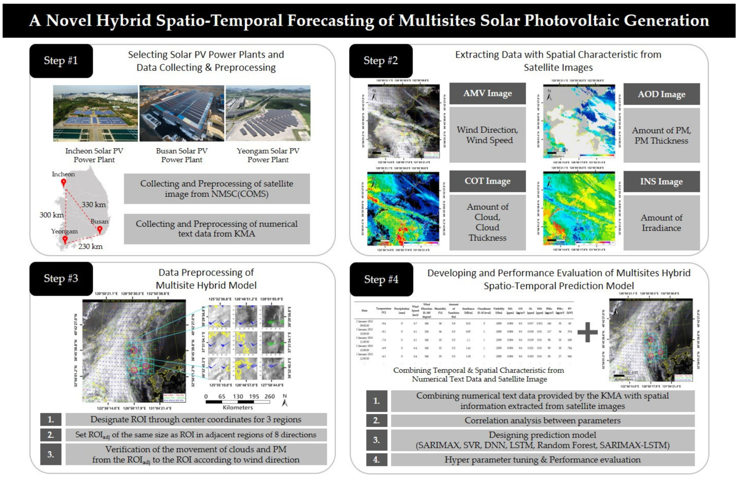
This study develops an hourly advanced multisite integrated hybrid spatio-temporal solar PV generation prediction model in South Korea. The prediction model uses meteorological numerical text data provided by the Korea Meteorological Agency (KMA) and spatial information data extracted from satellite images to reflect both temporal and spatial characteristics. By reflecting the spatio-temporal characteristics, higher prediction accuracy can be derived than the model using only existing numerical text data and satellite images. Figure 1 shows the overall flow of this study. The first step is to select solar PV power plants in three cities in South Korea, namely, Incheon, Busan, and Yeongam. A database (DB) was built by collecting and preprocessing meteorological information provided by the KMA in each region and satellite images provided by the National Meteorological Satellite Center (NMSC). The second step extracted the necessary spatial information from four satellite images. In the atmospheric motion vector (AMV) image, the wind direction vector and wind speed, the amount of cloud and thickness of the cloud in the cloud optical thickness (COT) image, the amount of PM and PM concentrations in the aerosol optical depth (AOD) image, and the amount of irradiance were extracted from the insolation (INS) image. The third step was to set the center coordinates for each region and the region of interest (ROI) around it. Furthermore, the ROI_adj is set to the same size as the ROI for the eight adjacent directions to the ROI. To learn spatial information from the solar PV generation prediction models, the effects of cloud and PM on wind direction were analyzed in ROI_adj and ROI. The fourth step was combining the meteorological numerical text data DB built in the first step and the data DB extracted from satellite images and performing a correlation analysis between each meteorological parameter, including clouds and PM, and the amount of solar PV generation. Finally, the fifth step was to develop predictions by applying the SARIMAX, traditional time-series analysis method, SVR, DNN, LSTM, Random Forest, and the SARIMAX-LSTM model, which incorporates the advantages of each method, for developing an hourly advanced multisite integrated hybrid spatio-temporal solar PV generation prediction model. Later, parameter optimization was performed for each technique to increase the prediction performance.

2. Methodology

2.1. Satellite Image Data

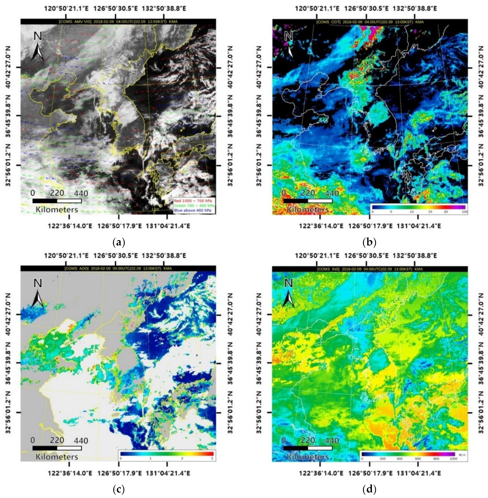
Herein, the solar PV generation prediction model should learn the spatial characteristics of each meteorological factor. Therefore, to extract spatial information, four years of satellite images from 2015 to 2018, from the Communication, Ocean, and Meteorological Satellite (COMS), were provided by the NMSC [30]. The COMS is South Korea’s first geostationary multipurpose satellite that provides meteorological and ocean observations and communication services. It was launched on 27 June 2010, from the Guiana Space Center. The COMS takes images of the Korean Peninsula of size 1024 × 1024 pixels and a spatial resolution of 1720.8 m per pixel. Every 15 min, 16 images are taken, including cloud detection, AMV, and surface temperature. In this study, four of the 16 types of images—AMV, COT, AOD, and INS images—were used [31,32,33,34]. Figure 2 shows each sample image at 13:00 on 9 February 2018. Each image’s description and methods for spatial information extraction are described in the subsections.

2.1.1. Atmospheric Motion Vector Image and Region of Interest

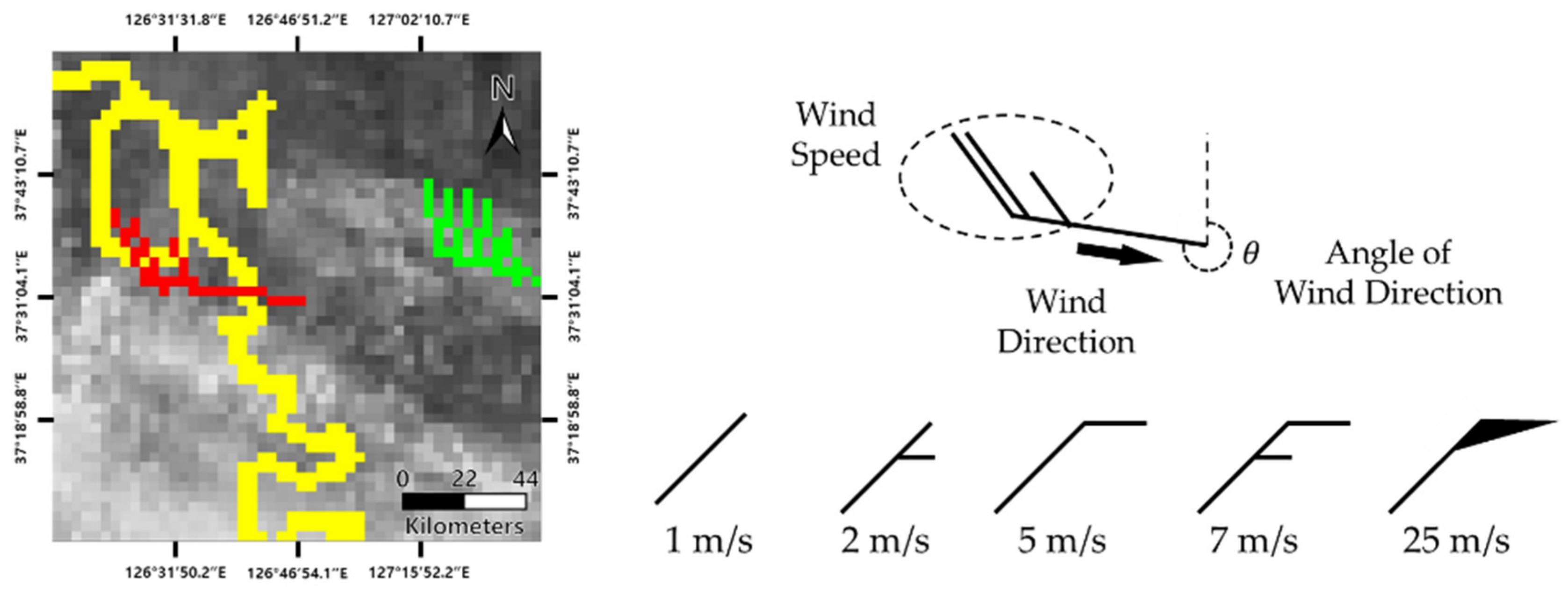
Clouds and PM significantly influence irradiance, a critical element of solar PV generation. Clouds and PM move along the wind. AMV images were used to show the effect on the spatial movement of clouds and PM. In Figure 2a, the AMV image shows the wind direction and wind speed information with arrows. The wind direction arrows are divided into red, green, and blue according to altitude. However, the AMV image does not provide numerical information on the wind direction vector. Therefore, to extract the wind direction and numerical information on the wind speed, we observed the following sequence. First, we selected the wind direction arrow closest to the target region and located the center coordinates of the wind direction arrow. The angle between the center coordinates and body of the wind direction arrow, as indicated by θ in Figure 3, was calculated to obtain the wind direction. Second, the wind direction can be calculated using the shape of the wing attached to the body of the wind direction arrow.

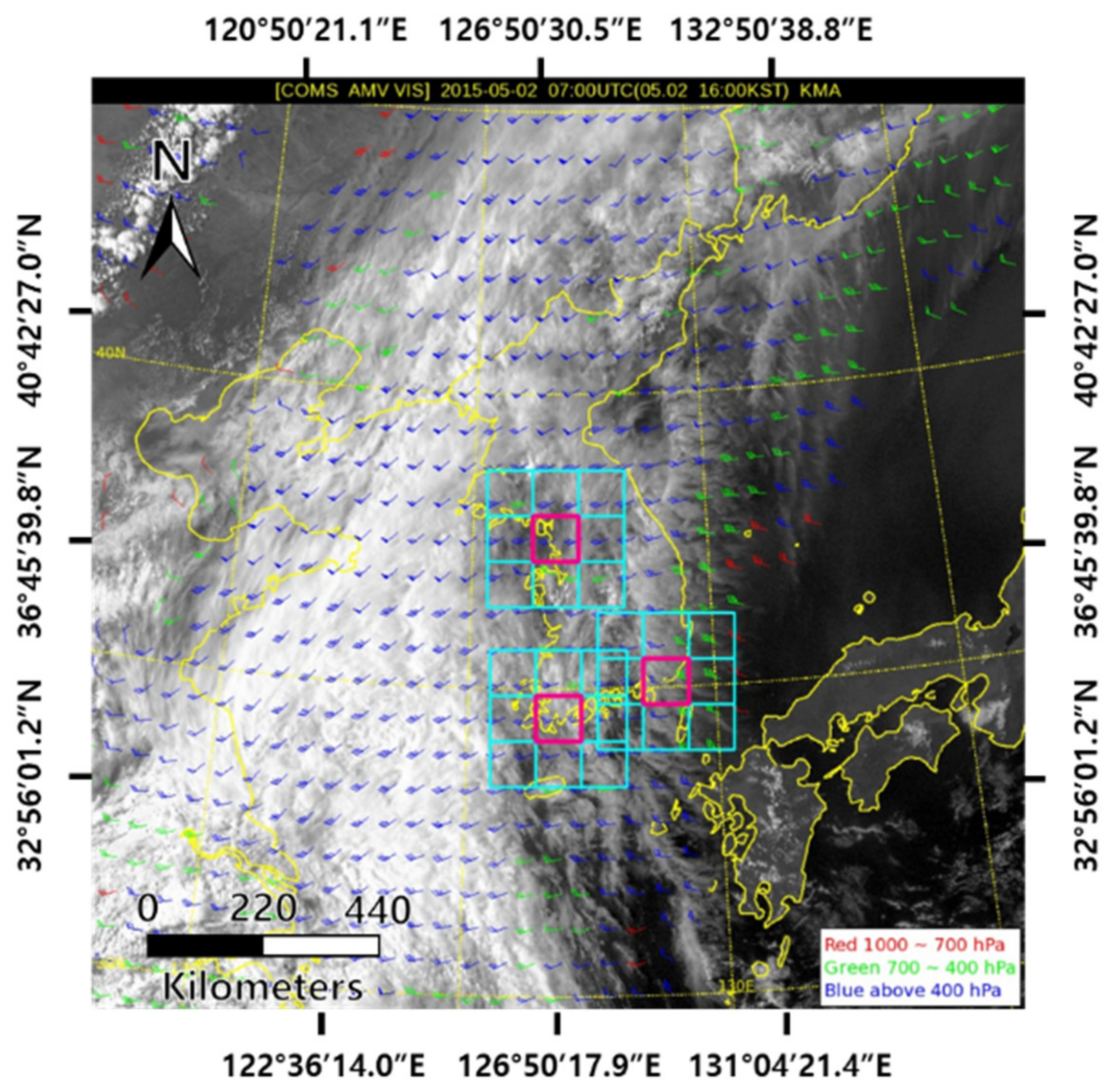
By setting the target region, where the solar PV power plant for predicting solar PV generation is located, as an ROI, the spatial characteristics of clouds and PM moving according to the wind direction were analyzed. The wind direction arrows in the AMV image rotate 360° around the center coordinates. Therefore, as the center coordinates of the wind direction arrow were fixed, the ROI is set to 50 × 50 pixels, which is a size that does not interfere with the wind direction arrow rotating with time. Furthermore, the impact on the surrounding region was identified by setting the ROI_adj for the eight adjacent directions around the ROI. Figure 4 shows the ROI and ROI_adj set in Incheon, Busan, and Yeongam in magenta and cyan, respectively.

2.1.2. Cloud Optical Thickness, Aerosol Optical Depth, and Insolation Images

Figure 2b–d show COT, AOD, and INS images, respectively. The COT image represents the thickness of the clouds through the color index in the bottom right corner, and information about the amount and thickness of clouds is extracted. The color indexes from 0 to 100 were divided into quarters and classified into clear, partly cloudy, mostly cloudy, and cloudy. Subsequently, the number of pixels for each index color belonging to the ROI and ROI_adj set through the AMV image was identified, and information about the cloud amount and thickness was saved. Similar to the COT image, the AOD image represents air pollutants, such as yellow dust and PM, as a color index. The color index is divided into good, moderate, bad, and very bad, and the PM amount and concentrations in the ROI and ROI_adj were saved. Finally, the INS image represents the amount of irradiance reaching the surface using the color index. To extract information about the amount of irradiance reaching the surface, the index information value for each pixel in the ROI was averaged and used.

Table 1. The sample of extracted cloud data from the cloud optical thickness image in the region of interest (Busan).

Date	Cloud				Particulate Matter				Irradiance
	Clear	Partly Cloudy	Mostly Cloudy	Cloudy	Good	Moderate	Bad	Very Bad
8 April 2015 09:00:00	1361	721	100	0	0	90	74	11	115.594
8 April 2015 11:00:00	763	1081	331	22	5	62	83	6	166.374
8 April 2015 12:00:00	456	741	799	224	25	74	0	0	136.422
8 April 2015 13:00:00	180	919	908	232	0	0	0	0	117.310
8 April 2015 14:00:00	436	1082	581	140	0	67	31	0	130.237
8 April 2015 15:00:00	887	894	411	31	13	96	48	0	132.545
8 April 2015 16:00:00	1369	629	168	13	153	197	59	22	117.817

shows the information extracted from three satellite images of the ROI in Busan.

2.2. Numerical Text Data

To predict the amount of hourly solar PV generation, three categories of numerical text data were used. Meteorological factors, such as temperature, humidity, and precipitation, air pollutants, such as PM₁₀ and PM_2.5, and solar PV generation data were used as parameters for predicting solar PV generation. The KMA, Air Korea, and the Open Data Portal provided the data [35,36,37], respectively. The KMA began meteorological observations in 1904 for meteorological stations in 103 regions across the country. Through this, more than 15 types of hourly data, such as temperature, precipitation, and humidity, are provided as public data. The location of the meteorological stations in each area used in the experiment was 37.4777658 lat. and 126.6223456 long. in Incheon and 35.2061563 lat. and 129.0806029 long. in Busan. Yeongam does not have a meteorological station, so the closest location, Mokpo, was used. The location of the meteorological station in Mokpo is 34.8171105 lat. and 126.3789376 long. Herein, temperature, humidity, cloudiness, wind speed, wind direction, precipitation, amount of sunlight, irradiance, and visibility were used as meteorological factors for predicting solar PV generation.

Air pollution caused by fossil fuels and the smoke of cars causes serious environmental problems. Increasing the PM concentration in the atmosphere not only harms the human body but also decreases the amount of irradiance by reducing visibility because of the effects of scattering and absorption when sunlight passes through the atmosphere. It significantly reduces solar PV generation. Therefore, Air Korea provided data for SO₂, CO, O₃, NO₂, PM₁₀, and PM_2.5, which were used as air pollution factors for predicting solar PV generation.

Finally, the Open Data Portal provided the most critical hourly solar PV generation data. Furthermore, data of latitude, longitude, and altitude were added to show the geographic information for each solar PV power plant, and facility capacity and installation angle information of solar panels were added to learn facility information. All data were collected for four years from 0:00 on 1 January 2015 to 23:00 on 31 December 2018. The k-nearest neighbors algorithm was used to interpolate missing values among the collected data, and interpolation was performed by learning data for 36 h before and after, i.e., 72 h based on the missing time point. The amount of irradiance, according to the daylight time, determines the amount of solar PV generation; hence, the daylight time of 24 h was set from 09:00 to 17:00.

Table 2. The capacity of each solar PV power plant and distance for each station.

Solar PV Power Plant	Capacity (kW)	Distance (km)
		Meteorological Station	Aerosol Station
Incheon	998.0	10.0	3.0
Busan	187.2	3.6	2.9
Yeongam	1491.6	12.7	5.0

summarizes the capacity of each solar PV power plant used in the study and the distance between each station.

Table 3. The sample of the numerical dataset.

Date	Temperature (°C)	Precipitation (mm)	Wind Speed (m/s)	Wind Direction (0–360 Degree)	Humidity (%)	Amount of Sunshine (h)	Irradiance (MJ/m2)	Cloudiness (0–10 Level)	Visibility (10 m)	SO2 (ppm)	CO (μg/m2)	O3 (ppm)	NO2 (ppm)	PM10 (μg/m2)	PM2.5 (μg/m2)	Capacity (kW)	Setting Angle (°)	Latitude (°)	Longitude (°)	Altitude (m)	PV (kW)
1 January 2015 09:00:00	−8.4	0	6.7	340	56	0.8	0.21	0	2000	0.006	0.5	0.017	0.012	145	33	998	20	37.26154	126.434	52	60
1 January 2015 10:00:00	−8.1	0	6.1	226	54	0	0.67	1	2000	0.006	0.5	0.019	0.01	117	34	998	20	37.26154	126.434	52	374
1 January 2015 11:00:00	−7.6	0	6.1	340	53	0	1.1	1	2000	0.006	0.6	0.019	0.01	98	33	998	20	37.26154	126.434	52	638
31 December 2018 15:00:00	−1.2	0	2.6	340	34	0.9	1.17	8	2000	0.006	0.6	0.024	0.026	47	15	998	20	37.26154	126.434	52	223
31 December 2018 16:00:00	−1.1	0	3.3	340	45	0.8	0.76	8	2000	0.006	0.6	0.021	0.03	40	16	998	20	37.26154	126.434	52	128
31 December 2018 17:00:00	−2.6	0	3	320	53	1	0.43	7	1680	0.005	0.6	0.023	0.024	39	13	998	20	37.26154	126.434	52	6

shows a sample of numerical text data from Incheon.

2.3. Parameter Analysis

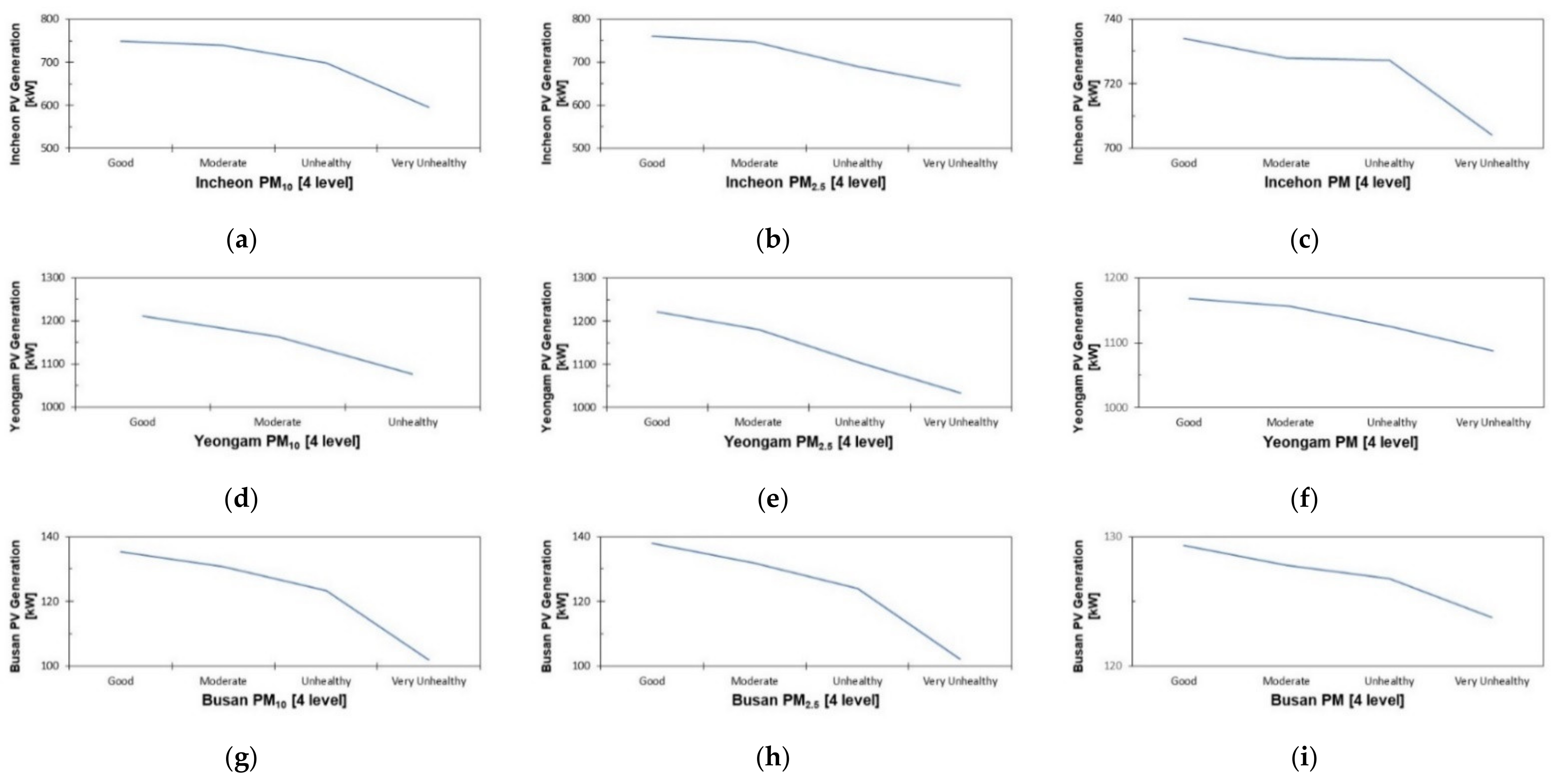
Pearson correlation analysis was conducted to analyze the correlation of parameters used to predict solar PV generation. Furthermore, additional validation was performed to analyze the effect of solar PV generation on clouds and PM of numerical text data provided by KMA and spatial information data extracted from satellite images. For clouds, the numerical text data comprise 0–10 levels, and the data extracted from the satellite image consist of four levels. For PM (

Table 4. The results of discriminant for movement of particulate matter by wind direction.

PM	Good	Moderate	Bad	Very Bad
PM10	0–30	31–80	81–150	150~
PM2.5	0–15	16–35	36–75	76~

), the numerical text data comprise four levels for both PM₁₀ and PM_2.5 according to the standards used in South Korea. The satellite image data were also analyzed by dividing them into four levels. To exclude the impact of each parameter as much as possible, when analyzing the effect on clouds, PM₁₀, and PM_2.5 were both at a good level, whereas when analyzing the effect on PM, the clouds used only 0–1 levels. Furthermore, the analysis was conducted for 2 h from 12:00 to 14:00, which is noon, when the highest amount of solar PV generation takes place. Figure 5 and Figure 6 show the graph of the correlation analysis results of the amount of solar PV generation for clouds and PM in each region. As the amount of clouds increases or the PM concentration increases, the amount of solar PV generation decreases.

As such, the spatial characteristics of each parameter are critical when learning the characteristics of clouds and PM, which significantly affect solar PV generation prediction. Therefore, spatial characteristics were verified using cloud and PM data extracted from satellite images and wind direction data extracted from AMV images. The verification methods are as follows. First, at time t, recognize the wind direction of the ROI. Next, the cloud and PM amounts are analyzed at time t of the ROI and each ROI_adj. Finally, depending on the wind direction, the increase or decrease because of the movement of clouds and PM is determined at the point t + 1 of the ROI. For example, assume that the wind direction is north, and the amounts of clouds in ROI and ROI_adj at time t are 5 and 8, respectively. At this time, when the amount of cloud of ROI is >5 at the time point t + 1, it is determined as true, and in the opposite case, it is determined as false.

Table 5. The results of cloud movement verification by wind direction.

Accuracy (%)	Clear	Partly Cloudy	Mostly Cloudy	Cloudy	Average
Incheon	73.008	78.354	85.692	93.947	82.750
Yeongam	75.401	78.457	84.792	91.644	82.574
Busan	73.680	79.529	85.662	93.896	83.192

and

Table 6. The results of particulate matter movement verification by wind direction.

Accuracy (%)	Good	Moderate	Bad	Very Bad	Average
Incheon	78.616	84.827	90.016	94.313	86.943
Yeongam	80.527	86.345	92.162	94.627	88.415
Busan	77.144	87.308	92.817	95.287	88.139

show the verified results.

3. Forecasting Solar PV Generation

3.1. Prediction Methods for Solar PV Generation

Various methods were used to predict the amount of solar PV generation. We used SARIMAX, a traditional statistical time-series analysis method, and SVR, a method that applies a loss function to the support vector machine (SVM), a representative classification algorithm. The DNN with high-level prediction performance was used by combining several nonlinear transformation techniques. As a method based on the decision tree method, a random forest model was used. The SARIMAX-LSTM model was used to create a new model by combining only the merits of each model and LSTM, which is easy for classification, processing, and prediction based on time-series data. Detailed descriptions of each method and model are provided in the following subsections.

3.1.1. Seasonal Autoregressive Integrated Moving Average with Exogenous Factors

The autoregressive integrated moving average (ARIMA) is a traditional statistical time-series analysis method developed by Newsham and Birt as a regression model that includes both the autoregressive (AR) model and the moving average (MA) model [38]. The AR model determines whether past data affect future data, and the MA model identifies a trend in which the average value of a random variable continuously increases or decreases with time. As the ARIMA is a univariate time-series model, the ARIMAX can manipulate multivariate time-series data by adding external factors to it. To apply the ARIMAX model, steady-state data are critical. If the data do not have a steady-state, the difference should be used to represent the steady state and then applied to the regression model.

The SARIMAX model adds seasonal characteristics to the ARIMAX model and can reflect the periodicity of the data [39]. The amount of solar PV generation, including the meteorological parameters used in the study, satisfies the steady-state and seasonal periodicity, as it has the characteristics of the four seasons and uses the hourly data. The SARIMAX model has the order of the nonseasonal AR (p), nonseasonal difference (d), nonseasonal MA (q), seasonal AR (P), seasonal difference (D), and seasonal MA (Q) order. In this study, SARIMAX (3, 0, 3) (3, 0, 3, 12)_s was used as the order for the solar PV generation prediction model.

3.1.2. Support Vector Regression

The SVM is a representative classification algorithm proposed by Vapnik in 1995 [40]. The SVR method introduces the loss function to SVM for regression analysis. The SVR must obtain an optimal regression function f(x) to minimize the difference between the actual and predicted values. To this end, the loss function reduces the size of the regression coefficient to find a line that flattens the regression equation and then determines all predicted values within a specific deviation ε called the support vector. The smaller the corresponding support vector, the more optimal the regression function f(x) that will be obtained. This is a typical linear regression method, but most data cannot solve the problem using only linear regression; a nonlinear regression equation should be used. The SVR can solve the problem by mapping the data of the existing input space into the feature space and using a mapping function that enables the data to be linearly expressed in a high-dimensional space. When data are mapped to a higher dimension, the regression equation becomes complex because of the curse of dimensionality, which significantly increases the computational amount. This problem can easily be solved using kernel functions, such as the radial basis function, linear, and polynomial kernels. The optimal regression function f(x) can be calculated by solving the Lagrangian problem through the dot product of the vector calculated using the kernel function. Herein, a linear kernel with the best prediction performance was used because of experimenting with various kernels of SVR models for solar PV generation prediction.

3.1.3. Deep Neural Network

Machine learning is used for classification and prediction in various fields [41]. The DNN consists of an input layer, a hidden layer, and an output layer, and more complex computation is possible by expanding the number of hidden layers in artificial neural networks (ANN) that mimic the human brain structure. The nodes at each DNN layer are interconnected, hence, they have the same effect as many neurons connected to collect and process multiple data in the human brain structure. By interacting with various nonlinear activation functions, such as Sigmoid, ReLU, and tanh in each DNN layer, the DNN model itself creates labels for each training data or distorts the space to derive optimal classification or prediction results. The conventional ANN method passes through the hidden layer from the input layer and proceeds in one direction to the output layer when calculating weights in a feed-forward method, rendering it impossible to adjust the weights. However, the prediction result’s precision can be improved by adopting the backpropagation algorithm, which computes the gradient earlier in the back layer using the gradient descent algorithm. If the number of hidden layers is simply increased to design the DNN model, the gradient might be stuck in the local minima, or a vanishing problem can occur, resulting in lower performance than a shallow ANN. Therefore, if the problem is solved using the dropout layer or applying a nonlinear activation function, higher performance prediction results can be derived by resolving vanishing gradient and overfitting problems.

Table 7. The structure of the DNN model.

Number of Hidden Layer	1	2	3	4	5	6	7
Number of Nodes	180	0.4	100	0.4	100	0.4	1
Activation Function	tanh	Drop out	ReLU	Drop out	Sigmoid	Drop out	Sigmoid

shows the structure of the DNN model used to predict solar PV generation in this study.

3.1.4. Long Short-Term Memory

The recurrent neural network (RNN) allows for effective analysis when data in the past have time-series characteristics because it can then consider sequence or temporal characteristics, through which past data can affect the future outcome [42]. Unlike other neural networks, the results of the hidden layer are linked so that they can revert to the input of the same hidden layer and share weights. However, the gradient-vanishing phenomenon, in which gradient values become exponentially smaller during the backpropagation process, and gradient expansion, in which gradient values grow exponentially during the learning process, do not accurately reflect long-term dependencies, and the model cannot proceed with learning.

Hochreiter and Schmidhuber proposed the LSTM, which can solve the long-term dependence problem of the RNN [43]. The LSTM has four layers of interaction, and through cell states, key information continues to be conveyed to the next level. Furthermore, the four layers use each gate element to add or remove various information. The gate that protects and controls the cell state is composed of forget gate, an input gate, and tanh layers, allowing information to flow selectively. It consists of a Sigmoid neural net layer and a point-by-point multiplication operation. The Sigmoid layer outputs a value of 0 or 1 to determine the effect of each component. If the output value is 0, the corresponding component does not affect the future. Conversely, when the output value is 1, the corresponding component influences the prediction result in the future.

Table 8. The structure of the LSTM model.

Number of Hidden Layer	1	2	3	4	5
Number of nodes	500	0.3	500	0.3	1
Activation function	LSTM	Drop out	Sigmoid	Drop out	tanh

shows the structure of the LSTM model used to predict solar PV generation in this study.

3.1.5. Random Forest

Random forest is an ensemble algorithm that learns multiple decision trees [44]. It is widely used in classification and regression problems because it can easily manage interactions and nonlinearities between parameters and is insensitive to outliers. The work of Yali Amit and Donald Geman [45] influenced the early concept of random forest, and Leo Breiman [46] established the present concept. Random forest can effectively prevent overfitting by adding the randomness of variable selection to the bagging method generating a model by randomly extracting a sample several times and iterating the restoration. It has high prediction stability because the average of the prediction results is used for numerous decision trees, and the optimal prediction value is derived by selecting the optimal decision tree model through a majority vote. Although prediction using a decision tree has a disadvantage because the prediction result or model performance fluctuates significantly, the randomization technique, which is a characteristic of the random forest, overcomes the disadvantage of the decision tree and has good generalization performance. The conventional random forest may be possible to cause the problem of concept drift, which deteriorates the performance of the predictive model over time. Hence, Zhukov et al. attempted to solve this problem [44]. In this study, 500 decision trees were used in the Random Forest model for solar PV generation prediction.

3.1.6. Ensemble Learning (SARIMAX-LSTM)

The key of ensemble learning is to achieve better generalization performance than individual weak learners by combining multiple single models to create one strong learner [47,48]. Representative ensemble techniques are classified into three methods. First, the bagging technique using the voting method randomly restores and extracts the target data. Using the extracted data as a sample group, the prediction results are aggregated as an average value after training each model, reducing errors in overfitting and underfitting caused by high variance or high bias. Second, the boosting technique using the weighted voting method applies weights in the restoration extraction process, unlike the bagging technique. Although the bagging technique proceeds with training in parallel, the boosting technique sequentially progresses; hence, weights are redistributed according to sequentially derived results in the training order with high accuracy. However, it has the disadvantage of being vulnerable to extreme outliers. Lastly, the stacking technique derives the performance of a new model by combining the advantages of different individual models. It adopts the characteristics of each model to highlight its advantages, complementing its disadvantages, which can improve performance over a single model.

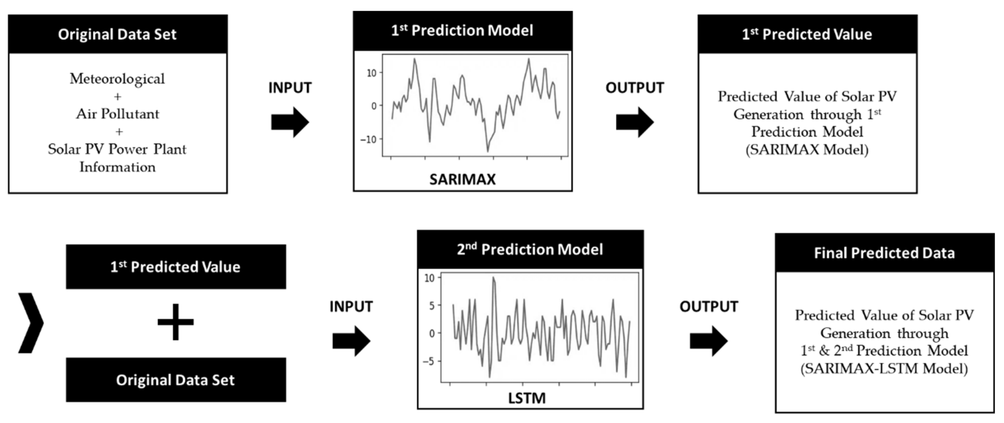
In this study, the stacking ensemble was used among various ensemble methods and the SARIMAX and LSTM models were used as weak learners to sequentially combine. This is to emphasize the time-series characteristics of various parameters, including meteorological factors, and solve the long and short-term dependency problem. Figure 7 shows the structure of the proposed SARIMAX-LSTM model. After the original data are derived from the SARIMAX model, the first result is derived, and the final predicted value is derived using it as the training data of the LSTM model.

3.2. Error Analysis for Prediction

Various methods exist to verify the error of the prediction model and can be classified into two methods: a relative error verification method and an absolute error verification method. Representative relative error verification methods are the mean square error (MAE) and the root mean square error (RMSE). The mean absolute percentage error is mainly used as an absolute error verification method. However, when the measured value is 0, it becomes infinite or undefined, and as the measured value converges to 0, it diverges to the limit. It also has the disadvantage of distorted results when there are many extreme outliers. In this study, the symmetric mean percentage error (SMAPE) was used to overcome these shortcomings. Each error verification method is expressed as Equations (1)–(3), and a value closer to 0 indicates that the model has superior performance.

Using the criteria of the American Society of Heating, Refrigerating, and Air-Conditioning Engineers (ASHRAE) Guideline 14 applied by energy managers to improve energy efficiency, we will additionally verify the performance of the solar PV generation prediction model [49]. For the objective evaluation of the solar PV generation prediction model, the mean bias error (MBE) and the coefficient of variation (Cv) criteria in the ASHRAE Guideline 14 were applied and are expressed as equations 4 and 5. For MBE, the performance increases as it converges to 0, regardless of the ± sign. However, in this study, absolute values have been taken for the results, thereby increasing intuition and convenience of comparison. From

Table 9. ASHRAE Guideline 14.

Calibration Type	Index	Acceptable Value
Monthly	MBE month	±5%
	Cv (RMSE) month	15%
Hourly	MBE hour	±10%
	Cv (RMSE) hour	30%

, according to the criteria of ASHRAE Guideline 14, the hourly prediction is defined within MBE ± 10% and Cv 30%.

$$MAE=\frac{1}{n}{\displaystyle \sum }_{i=1}^n\left|F_i-A_i\right|$$

(1)

$$RMSE=\sqrt{\frac{1}{n}{\displaystyle \sum }_{i=1}^n{\left(F_i-A_i\right)}^2}$$

(2)

$$SMAPE\left(\%\right)=\frac{1}{n}{\displaystyle \sum }_{i=1}^n\frac{\left|A_i-F_i\right|}{\left|A_i\right|+\left|F_i\right|}$$

(3)

$$MBE\left(\%\right)=\frac{{{\displaystyle \sum }}_{i=1}^n(F_i-A_i)}{{{\displaystyle \sum }}_{i=1}^n{A}_i}$$

(4)

$$Cv\left(\%\right)=\frac{RMSE}{\frac{1}{n}{{\displaystyle \sum }}_{i=1}^n{A}_i}$$

(5)

F: Forecast value, A: actual value, n: number of samples.

3.3. Cloud and PM Prediction for Solar PV Generation

Before predicting solar PV generation, clouds and PM are first predicted to reflect their spatial characteristics. During the entire experimental period, 2015–2018, the clouds and PM in the ROI and ROI_adj were learned using satellite images data from 2015 to 2017. It then predicts the hourly cloud and PM of ROI in 2018. To predict clouds and PM, data extracted from satellite images and numerical text data for meteorological factors and air pollutant factors were combined and used. The LSTM model for clouds and PM was used differently from the solar PV generation prediction LSTM model. Table 1 and Table 3 show the input parameters. Here, 15 parameters are used in Table 3, excluding the solar PV power plant’s facilities and geographical factors.

Table 10. The structure of the LSTM model for clouds and PM prediction.

Number of Hidden Layer	1	2	3
Number of nodes	500	0.3	1
Activation function	LSTM	Drop out	ReLU

shows the structure of the LSTM model used to predict clouds and PM in this study.

Table 11. The results of clouds and PM prediction.

Region	Error	Cloudiness	PM10	PM2.5
Incheon	MAE	0.977	8.248	4.223
	RMSE	1.383	14.425	6.356
	SMAPE (%)	7.701	11.601	14.729
Yeongam	MAE	1.640	7.014	5.748
	RMSE	2.040	10.007	7.626
	SMAPE (%)	11.734	10.644	13.506
Busan	MAE	1.238	7.215	4.612
	RMSE	1.595	11.266	6.197
	SMAPE (%)	9.681	8.692	11.010

shows the prediction results.

3.4. Proposed Model for Solar PV Generation

To predict hourly solar PV generation, the prediction model is learned using various meteorological parameters, including the predicted cloud amount and PM. Furthermore, to reflect the temporal characteristics in the prediction model, variables representing time, such as the month, day, and time, were added. To predict the amount of solar PV generation, the 2018 data were divided into training, verification, and test data ratio of 3:1:1 for each month. Five models were used for prediction: SARIMAX, SVR (Line kernel), DNN, LSTM, Random Forest, and SARIMAX-LSTM.

Table 12. The parameters of the solar PV generation prediction model.

Data	Parameters
Input	Year, Month, Day, Time, Temperature, Precipitation, Wind speed (numerical text data & satellite image data), Wind direction (numerical text data & satellite image data), Humidity, Amount of sunshine, Irradiance (numerical text data & satellite image data), Cloudiness, Visibility, SO2, CO, O3, NO2, PM10, PM2.5, Clouds (clear, partly cloudy, mostly cloudy, cloudy), PM (good, moderate, bad, very bad), Capacity, Setting angle, Latitude, Longitude, Altitude, PV (previous data)
Output	PV (one hour ahead)

shows the parameters for forecasting the amount of solar PV generation.

4. Experimental Results

To compare the performance of the single-site and multisite solar PV generation prediction models, 21 of 36 parameters were validated, excluding the facilities and geographic parameters of a single-site solar PV generation prediction model used in the results of a previous study [23].

Table 13. The results of the single-site solar PV generation model using the multisite data set.

Error	ARIMAX	SVR_RBF	SVR_Linear	ANN	DNN
MAE	76.176	225.020	87.082	584.648	80.959
RMSE	107.102	269.205	113.624	643.798	113.724
SMAPE	24.709	43.406	28.900	99.996	23.330
MBE	2.806	18.103	1.921	182.612	2.926
Cv	33.453	84.085	35.490	201.087	35.521

shows the results of the evaluation by applying the data of three regions to the previous study, the single-site solar PV generation prediction model. Based on the absolute evaluation method SMAPE, the prediction performance was excellent in the order of DNN model, ARIMAX model, SVR_Linear model, SVR_RBF model, and ANN model. Among all five models, the ARIMAX, which manages multivariate time-series data, was the best in all error verification methods, except the SMAPE and MBE. The ARIMAX model predicts by showing the time-series characteristics; hence, it has a certain level of predictive performance, but does not have optimal performance. The SVR_Linear model, including the ARIMAX and DNN models, shows satisfactory performance, whereas the ANN model shows severe performance degradation. However, all five models did not meet the criteria of ASHRAE Guideline 14.

Table 14. The multisite solar PV generation prediction results of the proposed model.

Error	SARIMAX	SVR_Linear	LSTM	DNN	Random Forest	SARIMAX-LSTM
MAE	76.169	84.791	76.913	70.378	69.812	64.730
RMSE	102.575	109.130	106.123	101.783	106.226	95.800
SMAPE	27.743	29.155	23.369	22.365	18.364	19.891
MBE	1.346	2.752	2.985	5.312	3.323	2.650
Cv	32.039	34.086	33.147	31.791	33.179	29.923

shows the prediction results of the five models proposed for multisite solar PV generation in this study. Based on the SMAPE, the prediction performance was excellent in the order of Random Forest model, SARIMAX-LSTM model, DNN model, LSTM model, SARIMAX model, and SVR_Linear model. The Random Forest model has the best performance based on the SMAPE, but does not meet the ASHRAE Guideline 14. For the SARIMAX model, the performance is increased compared to the ARIMAX model. Compared with the existing model, the SVR_Linear and DNN models show an increase in performance of 3.96 and 10.5%, respectively, based on RMSE. Although the performance of the LSTM model is low compared to the newly proposed DNN model, it has the best performance of all proposed models for the SARIMAX-LSTM model combined with the SARIMAX model by applying the stacking ensemble technique. Furthermore, the SARIMAX-LSTM model has MBE: 2.65; Cv: 29.92, which is the only one of 10 models meeting the criteria of ASHRAE Guideline 14.

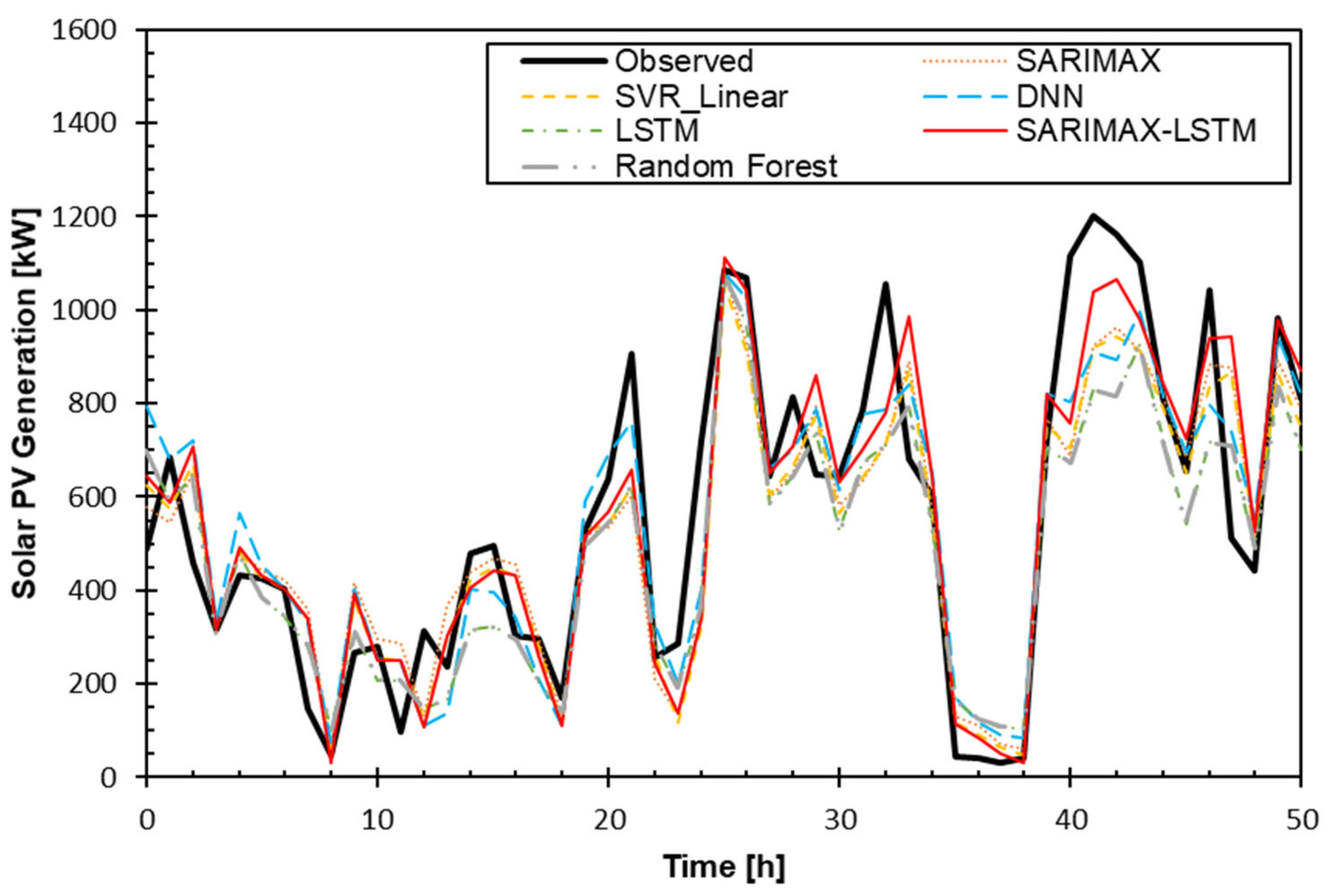
Figure 8 shows 50 h of the overall prediction results of the SARIMAX, SVR_Linear, LSTM, DNN, Random Forest, and SARIMAX-LSTM models. The thick black line is the original observation value and has a value similar to the predicted result of the overall model. The SARIMAX-LSTM model marked with solid red lines shows that it has superior performance to the other models.

5. Discussion

The single-site solar PV generation prediction model has limitations when using multisite data. The ARIMAX model shows the multivariate time-series characteristics in a single-site solar PV generation prediction model, and the SARIMAX model in a multisite solar PV generation prediction model, show higher performance than the other models but do not fulfill the criteria of ASHRAE Guideline 14. The performance of the single-site solar PV generation prediction model using multisite data set is similar to the performance of the multisite solar PV generation prediction model but does not have the optimal results because the single-site solar PV generation prediction model cannot learn on several factors, including the facility and geographic information of the solar PV power plants included in the multisite data. To improve the performance of the proposed model, finding and improving the factors hindering the prediction performance is necessary. The inhibitory factor is deemed the missing value of the AMV data. In the preprocessing step, after recognizing the wind direction arrow image of the AMV image, one must proceed to the next step. However, in this case, if there are no wind direction data in the ROI in the entire AMV image, the corresponding time zone is recognized as a missing value because there is no wind direction arrow. Therefore, if the number of missing values can be reduced when using various interpolation methods or extracting satellite image data using other methods, more improved models could have better performance.

6. Conclusions

This study proposed an advanced multisite integrated hybrid spatio-temporal solar PV generation prediction model by combining time-series-based meteorological numerical text and satellite image data with spatial information to develop a precise and accurate prediction model for solar PV power plants in multiple regions. The existing data provided by the KMA contain time-series characteristics but do not reflect the spatial characteristics of clouds and PM moving according to the wind direction. Therefore, data on clouds and PM moving according to the wind direction were extracted using satellite images to show the spatial characteristics together. It predicted the solar PV generation of existing solar PV power plants in both single and other regions. The data from 2015 to 2018 were used for three solar PV power plants in Incheon, Busan, and Yeongam in South Korea. To reflect the spatial characteristics of clouds and PM, the data from 2015 to 2017 were learned in order to predict the number of clouds and PM in 2018 first, and the amount of solar PV generation in 2018 was predicted using the predicted cloud and PM data. To develop the optimal prediction model, SARIMAX, a traditional time-series analysis method, and SVR_Linear, DNN, LSTM, Random Forest, and SARIMAX-LSTM models based on machine learning algorithms were used.

Consequently, the overall performance increased compared to the single-site solar PV generation prediction model. For the SARIMAX-LSTM model to which the stacking ensemble technique was used to make the most of the temporal characteristics of the solar power generation data, the results were MAE: 64.730; RMSE: 95.800; SMAPE: 19.891; MBE: 2.650; and Cv: 29.923. Among the proposed models, it is the only model that satisfies ASHRAE Guideline 14 and showed the best performance.

The proposed advanced multisite integrated hybrid spatio-temporal solar PV generation prediction model can predict integrated solar PV power generation for solar PV power plants in various regions in South Korea using numerical text data and satellite images. Therefore, it enables the prediction of solar PV generation for both existing and newly constructed solar PV power plants. By learning the facility and geographic information of each solar PV power plant, and the meteorological and air pollutant data of the area where the solar PV power plant is located, the amount of solar PV generation can be predicted. This reflects the spatio-temporal characteristics of solar PV generation, thereby providing guidelines for developing a precise and accurate solar PV generation prediction model for a stable power supply and demand plan.

References

1. Höök, M.; Tang, X. Depletion of fossil fuels and anthropogenic climate change—A review. Energy Policy 2013, 52, 797–809. [Google Scholar] [CrossRef] [Green Version]
2. Horowitz, C.A. Climate change. Nature 2011, 479, 267–268. [Google Scholar] [CrossRef] [Green Version]
3. Horowitz, C.A. Paris agreement. Int. Leg. Mater. 2016, 55, 740–755. [Google Scholar] [CrossRef]
4. IRENA. Energy and Renewable Energy 3020 Plan; IEA: Paris, France, 2017. [Google Scholar]
5. Haegel, N.M.; Margolis, R.; Buonassisi, T.; Feldman, D.; Froitzheim, A.; Garabedian, R.; Green, M.; Glunz, S.; Henning, H.-M.; Holder, B.; et al. Terawatt-scale photovoltaics: Trajectories and challenges. Science 2017, 356, 141–143. [Google Scholar] [CrossRef]
6. Renewable Energy Statistics. Korea Ministry of Trade, Industry and Energy. 2014. Available online: http://www.motie.go.kr (accessed on 9 May 2021).
7. Tyagi, V.; Rahim, N.A.; Rahim, N.A.; Jeyraj, A.; Selvaraj, L. Progress in solar PV technology: Research and achievement. Renew. Sustain. Energy Rev. 2013, 20, 443–461. [Google Scholar] [CrossRef]
8. Fang, X.; Misra, S.; Xue, G.; Yang, D. Smart grid—The new and improved power grid: A survey. IEEE Commun. Surv. Tutor. 2012, 14, 944–980. [Google Scholar] [CrossRef]
9. Kang, H. An analysis of the causes of fine dust in Korea considering spatial correlation. Environ. Resour. Econ. Rev. 2019, 28, 327–354. [Google Scholar] [CrossRef]
10. Peters, I.M.; Karthik, S.; Liu, H.; Buonassisi, T.; Nobre, A. Urban haze and photovoltaics. Energy Environ. Sci. 2018, 11, 3043–3054. [Google Scholar] [CrossRef] [Green Version]
11. Darwish, Z.A.; Kazem, H.A.; Sopian, K.; Al-Goul, M.; Alawadhi, H. Effect of dust pollutant type on photovoltaic performance. Renew. Sustain. Energy Rev. 2015, 41, 735–744. [Google Scholar] [CrossRef]
12. Maghami, M.R.; Hizam, H.; Gomes, C.; Radzi, M.A.; Rezadad, M.I.; Hajighorbani, S. Power loss due to soiling on solar panel: A review. Renew. Sustain. Energy Rev. 2016, 59, 1307–1316. [Google Scholar] [CrossRef] [Green Version]
13. Hiyama, T.; Kitabayashi, K. Neural network based estimation of maximum power generation from PV module using environmental information. IEEE Power Eng. Rev. 1997, 17, 241–247. [Google Scholar] [CrossRef]
14. Chow, S.K.; Lee, E.W.; Li, D.H. Short-term prediction of photovoltaic energy generation by intelligent approach. Energy Build. 2012, 55, 660–667. [Google Scholar] [CrossRef]
15. Liu, L.; Zhao, Y.; Chang, D.; Xie, J.; Ma, Z.; Sun, Q.; Yin, H.; Wennersten, R. Prediction of short-term PV power output and uncertainty analysis. Appl. Energy 2018, 228, 700–711. [Google Scholar] [CrossRef]
16. Kim, G.; Choi, J.H.; Park, S.Y.; Bhang, B.G.; Nam, W.J.; Cha, H.L.; Park, N.; Ahn, H.-K. Prediction model for PV performance with correlation analysis of environmental variables. IEEE J. Photovoltaics 2019, 9, 832–841. [Google Scholar] [CrossRef]
17. Monfared, M.; Fazeli, M.; Lewis, R.; Searle, J. Day-ahead prediction of pv generation using weather forecast data: A case study in the UK. In Proceedings of the 2nd Intetnational Conference on Electrical, Communication and Computer Engineering (ICECCE), Istanbul, Turkey, 12–13 June 2020. [Google Scholar] [CrossRef]
18. Dev, S.; Savoy, F.M.; Lee, Y.H.; Winkler, S. Short-term prediction of localized cloud motion using ground-based sky imagers. In Proceedings of the 2016 IEEE Region 10 Conference (TENCON), Singapore, 22–25 November 2016; pp. 2563–2566. [Google Scholar]
19. Cheng, H.-Y. Cloud tracking using clusters of feature points for accurate solar irradiance nowcasting. Renew. Energy 2017, 104, 281–289. [Google Scholar] [CrossRef]
20. Jang, H.S.; Bae, K.Y.; Park, H.-S.; Sung, D.K. Solar Power Prediction Based on Satellite Images and Support Vector Machine. IEEE Trans. Sustain. Energy 2016, 7, 1255–1263. [Google Scholar] [CrossRef]
21. Chow, C.W.; Urquhart, B.; Lave, M.; Dominguez, A.; Kleissl, J.; Shields, J.; Washom, B. Intra-hour forecasting with a total sky imager at the UC San Diego solar energy testbed. Sol. Energy 2011, 85, 2881–2893. [Google Scholar] [CrossRef] [Green Version]
22. Catalina, A.; Torres-Barrán, A.; Alaíz, C.M.; Dorronsoro, J.R. Machine learning nowcasting of PV energy using satellite data. Neural Process. Lett. 2020, 52, 97–115. [Google Scholar] [CrossRef]
23. Kim, B.; Suh, D. A Hybrid spatio-temporal prediction model for solar photovoltaic generation using numerical weather data and satellite images. Remote Sens. 2020, 12, 3706. [Google Scholar] [CrossRef]
24. Khandakar, A.; Chowdhury, M.E.H.; Kazi, M.-K.; Benhmed, K.; Touati, F.; Al-Hitmi, M.; Gonzales, A.J.S.P. Machine learning based photovoltaics (PV) power prediction using different environmental parameters of Qatar. Energies 2019, 12, 2782. [Google Scholar] [CrossRef] [Green Version]
25. Preda, S.; Oprea, S.-V.; Bâra, A.; Belciu, A. PV Forecasting using support vector machine learning in a big data analytics context. Symmetry 2018, 10, 748. [Google Scholar] [CrossRef] [Green Version]
26. Ahmad, M.W.; Mourshed, M.; Rezgui, Y. Tree-based ensemble methods for predicting PV power generation and their comparison with support vector regression. Energy 2018, 164, 465–474. [Google Scholar] [CrossRef]
27. Vagropoulos, S.I.; Chouliaras, G.I.; Kardakos, E.G.; Simoglou, C.K.; Bakirtzis, A.G. Comparison of SARIMAX, SARIMA, modified SARIMA and ANN-based models for short-term PV generation forecasting. In Proceedings of the 2016 IEEE International Energy Conference (ENERGYCON), Leuven, Belgium, 4–8 April 2016; pp. 8–13. [Google Scholar] [CrossRef]
28. Gensler, A.; Henze, J.; Sick, B.; Raabe, N. Deep Learning for Solar Power Forecasting—An Approach Using AutoEncoder and LSTM Neural Networks. In Proceedings of the 2016 IEEE International Conference on Systems, Man and Cybernetics (SMC 2016), Budapest, Hungary, 9–12 October 2017; pp. 2858–2865. [Google Scholar] [CrossRef]
29. Liu, F.; Li, R.; Li, Y.; Yan, R.; Saha, T. Takagi–Sugeno fuzzy model-based approach considering multiple weather factors for the photovoltaic power short-term forecasting. IET Renew. Power Gener. 2017, 11, 1281–1287. [Google Scholar] [CrossRef]
30. National Meteorogical Satellite Center. Available online: https://nmsc.kma.go.kr/ (accessed on 9 May 2021).
31. N.M.S. Center. Atmospheric Motion Vector Algorithm Theoretical Basis; NMSC National Meteorological Satellite Center: Guam-gil, Korea, 2012.
32. N.M.S. Center. COT Algorithm Theoretical Basis Document; NMSC National Meteorological Satellite Center: Guam-gil, Korea, 2012.
33. N.M.S. Center. AOD Algorithm Theoretical Basis Document; NMSC National Meteorological Satellite Center: Guam-gil, Korea, 2012.
34. N.M.S. Center. INS Algorithm Theoretical Basis Document; NMSC National Meteorological Satellite Center: Guam-gil, Korea, 2012.
35. Korea Meteorolgical Administration. Available online: https://data.kma.go.kr/ (accessed on 9 May 2021).
36. Air Korea. Available online: https://www.airkorea.or.kr/ (accessed on 9 May 2021).
37. Open Data Portal. Available online: https://www.data.go.kr/ (accessed on 9 May 2021).
38. Newsham, G.R.; Birt, B.J. Building-level occupancy data to improve ARIMA-based electricity use forecasts. In Proceedings of the 2nd ACM Workshop Embedded Sensing Systems Energy-Efficiency in Building, Zurich, Switzerland, 2 November 2010; pp. 13–18. [Google Scholar] [CrossRef] [Green Version]
39. Sheng, F.; Jia, L. Short-term load forecasting based on SARIMAX-LSTM. In Proceedings of the 5th International Conference on Power Renewable Energy (ICPRE), Shanghai, China, 12–14 September 2020; pp. 90–94. [Google Scholar] [CrossRef]
40. Cortes, C.; Vapnik, V. Support-vector networks. Mach. Learn. 1995, 20, 273–297. [Google Scholar] [CrossRef]
41. Kalogirou, S.A. Artificial neural networks in renewable energy systems applications: A review. Renew. Sustain. Energy Rev. 2000, 5, 373–401. [Google Scholar] [CrossRef]
42. Biehl, M. Supervised sequence labelling with recurrent neural neural networks. Neural Netw. 2005, 1999, 160. Available online: http://www.amazon.com/Supervised-Labelling-Recurrent-Computational-Intelligence/dp/3642247962 (accessed on 9 May 2021).
43. Greff, K.; Srivastava, R.K.; Koutnik, J.; Steunebrink, B.R.; Schmidhuber, J. LSTM: A search space odyssey. IEEE Trans. Neural Netw. Learn. Syst. 2017, 28, 2222–2232. [Google Scholar] [CrossRef] [Green Version]
44. Zhukov, A.V.; Sidorov, D.N.; Foley, A.M. Random forest based approach for concept drift handling. Commun. Comput. Inf. Sci. 2017, 661, 69–77. [Google Scholar] [CrossRef] [Green Version]
45. Amit, Y.; Geman, D. Shape quantization and recognition with randomized trees. Neural Comput. 1997, 9, 1545–1588. [Google Scholar] [CrossRef] [Green Version]
46. Breiman, L. Random forests. Random For. 2001, 45, 5–32. [Google Scholar] [CrossRef]
47. Kwon, H.; Ruy, W. A study on the work-time estimation for block erections using stacking ensemble learning. J. Soc. Nav. Archit. Korea 2019, 56, 488–496. [Google Scholar] [CrossRef]
48. Lee, S.; Kim, H. A new ensemble machine learning technique with multiple stacking. J. Soc. E-Bus. Stud. 2020, 25, 1–13. [Google Scholar]
49. ANSI/ASHRAE. ASHRAE Guideline 14-2002 Measurement of Energy and Demand Savings; 2002; Volume 8400, p. 170. Available online: http://www.eeperformance.org/uploads/8/6/5/0/8650231/ashrae_guideline_14-2002_measurement_of_energy_and_demand_saving.pdf (accessed on 9 May 2021).
Figure 1. The research framework of this study.
Remotesensing 13 02605 g001
Figure 2. Four satellite images at 13:00 on 28 February 2016: (a) atmospheric motion vector image; (b) cloud optical thickness image; (c) aerosol optical depth image; (d) insolation image.
Remotesensing 13 02605 g002
Figure 3. A standard station model for wind direction and speed.
Remotesensing 13 02605 g003
Figure 4. The region of interest (ROI) and ROIadj for Incheon, Busan, and Yeongam in the atmospheric motion vector image.
Remotesensing 13 02605 g004
Figure 5. The reduction rates of solar PV generation according to cloudiness: (a) The reduction rates in Incheon (KMA); (b) The reduction rates in Incheon (NMSC); (c) The reduction rates in Yeongam (KMA); (d) The reduction rates in Yeongam (NMSC); (e) The reduction rates in Busan (KMA); (f) The reduction rates in Busan (NMSC).
Remotesensing 13 02605 g005
Figure 6. The reduction rates of solar PV generation according to particulate matter (PM): (a) The reduction rates in Incheon (KMA PM10); (b) The reduction rates in Incheon (KMA PM2.5); (c) The reduction rates in Incheon (NMSC PM); (d) The reduction rates in Yeongam (KMA PM10); (e) The reduction rates in Yeongam (KMA PM2.5); (f) The reduction rates in Yeongam (NMSC PM); (g) The reduction rates in Busan (KMA PM10); (h) The reduction rates in Busan (KMA PM2.5); (i) The reduction rates in Busan (NMSC PM).
Remotesensing 13 02605 g006
Figure 7. The architecture of the SARIMAX-LSTM model.
Remotesensing 13 02605 g007
Figure 8. The result of multisite solar PV generation prediction of each model.
Remotesensing 13 02605 g008