Mixed Noise Estimation Model for Optimized Kernel Minimum Noise Fraction Transformation in Hyperspectral Image Dimensionality Reduction

Abstract

Dimensionality reduction (DR) is of great significance for simplifying and optimizing hyperspectral image (HSI) features. As a widely used DR method, kernel minimum noise fraction (KMNF) transformation preserves the high-order structures of the original data perfectly. However, the conventional KMNF noise estimation (KMNF-NE) uses the local regression residual of neighbourhood pixels, which depends heavily on spatial information. Due to the limited spatial resolution, there are many mixed pixels in HSI, making KMNF-NE unreliable for noise estimation and leading to poor performance in KMNF for classification on HSIs with low spatial resolution. In order to overcome this problem, a mixed noise estimation model (MNEM) is proposed in this paper for optimized KMNF (OP-KMNF). The MNEM adopts the sequential and linear combination of the Gaussian prior denoising model, median filter, and Sobel operator to estimate noise. It retains more details and edge features, making it more suitable for noise estimation in KMNF. Experiments using several HSI datasets with different spatial and spectral resolutions are conducted. The results show that, compared with some other DR methods, the improvement of OP-KMNF in average classification accuracy is up to 4%. To improve the efficiency, the OP-KMNF was implemented on graphics processing units (GPU) and sped up by about 60× compared to the central processing unit (CPU) implementation. The outcome demonstrates the significant performance of OP-KMNF in terms of classification ability and execution efficiency.

1. Introduction

Hyperspectral remote sensing combines imaging technology and spectroscopy technology to obtain continuous and narrow-band image data with high spectral resolution [1], which improves the ability to monitor the Earth’s systems and human activities [2,3]. However, the high-dimensional data obtained by the hyperspectral sensor are challenging to analyse and apply [4,5]. In hyperspectral image (HSI) classification, with limited training samples, the classifier performance first improves as the dimension increases but degrades when the dimension is higher than an optimal value (the Hughes phenomenon) [6,7]. Dimensionality reduction (DR) is a powerful tool to solve this problem and has become a critical step in HSI processing tasks because of its effectiveness at simplifying and optimizing HSI features [8].

DR methods are generally divided into two major categories: band selection and feature extraction. Band selection methods select a subset of spectral features from the original data [9,10]. These methods can be split into six groups [11]: ranking-based methods [12,13,14], search-based methods [15,16], clustering-based methods [17,18,19], sparsity-based methods [20,21,22], embedding-learning-based methods [11], and hybrid-scheme-based methods [23,24,25]. Although band selection retains valuable bands for subsequent processing, the algorithms have a large computational burden and often are not robust in complex scenes. Moreover, it is difficult to determine the optimal number of bands [11]. Unlike band selection, the feature extraction methods transform the original data into an optimized feature space with mathematical manipulation [26]. These methods can be divided into two classes. The first class consists of linear feature extraction methods such as non-negative matrix factorization (NMF) [27], non-negative matrix underapproximation (NMU) [28], linear discriminant analysis (LDA) [29], principal component analysis (PCA) [30], and minimum noise fraction (MNF) transformation [31]. The second class consists of non-linear feature extraction methods, which can be categorized into three groups: manifold-learning-based methods [32,33,34], graph-theory-based methods [35], and kernel-based methods [36,37]. NMF preserves the non-negativity of HSIs in low-dimensional space by imposing the nonnegative constrain. NMU is closely related to NMF but enables a recursive procedure for NMF and has the advantage of identifying features sequentially. However, both NMF and NMU ignore the intrinsic geometric structure information of data, which makes it difficult to obtain the desired results when the data are nonlinear [38]. LDA is a practical subspace technology that concentrates on mathematically manipulating the original high-dimensional space to a lower-dimensional space, where the class separation is maximized [29]. This method needs to annotate the data firstly, which undoubtedly increases the workload for the DR process. PCA is an orthogonal linear transformation based on information content, yet when the noise is unevenly distributed in each band, it cannot guarantee that the components are arranged following the image quality [31]. In contrast, the components are sorted by image quality after MNF transformation, no matter how the noise distributes in each band [31].

Due to factors such as the absorption and scattering of the atmosphere, and the interaction of terrain objects within a pixel in the imaging process, there are non-linear characteristics inherent in HSI [39]. The linear feature extraction methods mentioned above cannot handle the non-linear characteristics of data excellently. Kernel MNF (KMNF) transformation is proposed to solve this problem in MNF. As a kernel-based method, KMNF adopts kernel functions to transform the original data from the input space to the high-dimensional feature space to ensure data linear separability, and then, the non-linear features can be effectively extracted. Because of the kernel functions in KMNF, the computational complexity increased and the execution efficiency was reduced [38,40,41]. Although KMNF is widely used in non-linear feature extraction, it has been shown that KMNF cannot produce the expected results because of the inaccurate noise estimation [5,26,42,43]. The conventional MNF noise estimation (MNF-NE) and KMNF noise estimation (KMNF-NE) utilize the residual of a local regression in 3 $\times$ 3 neighbourhood pixels to a paraboloid or a plane, which depends heavily on the relationship between adjacent pixels [38,44]. The pixels obtained by hyperspectral sensors are mixtures of terrain objects located in the field of view. Due to the limited spatial resolution, there are many mixed pixels in HSI, making the spatial information unreliable for noise estimation [26]. In order to solve this problem in MNF, Gao et al. proposed optimized MNF (OMNF) employing spectral and spatial decorrelation (SSDC) to produce more precise noise estimation and significant improvements in MNF for classification [2,42,45,46]. Like OMNF, Gao et al. proposed an optimized KMNF (OKMNF), which used SSDC to improve the noise estimation during KMNF [26]. It was found that OKMNF is unsuitable for processing HSIs with complex scenes due to the weakness of SSDC in estimating noise. Zhao et al. introduced image segmentation to improve the performance of KMNF, which combines the spectral decorrelation and the spatial information of a homogeneous region generated by image segmentation to estimate noise. It produced better results than KMNF but was more time-consuming [5].

For instrumental noise and atmospheric effects, HSIs often suffer from annoying degradations during the imaging process by a mixture of various types of noise that include thermal noise, quantization noise, and sparse noise. Thermal noise and quantization noise in HSI is subject to Gaussian additive noise, which is signal-independent. Due to the imperfect instrument, sparse noise such as missing pixels, salt and pepper noise, and other outliers often exist in HSI [47]. In terms of the inaccurate noise estimation in KMNF and considering the types of noise in HSIs, this paper proposes a mixed noise estimation model (MNEM) during KMNF for optimized KMNF (OP-KMNF). Instead of using the residual of a local regression in the nearest neighbourhood pixels, the MNEM adopts the sequential and linear combination of the Gaussian prior denoising model, the median filter, and the Sobel operator to estimate noise during KMNF. To improve the execution efficiency, the OP-KMNF is implemented on graphics processing units (GPU). It achieves significant acceleration compared to the central processing unit (CPU) implementation.

It is worthwhile highlighting several aspects of the proposed method here: (1) aiming at the problem of inaccurate noise estimation during KMNF transformation, a new noise estimation method, MNEM, that is more suitable for noise estimation in KMNF is proposed. It is more effective and more robust, retains more details and edge features, and is more suitable than KMNF-NE and SSDC for noise estimation in KMNF. Experimental results, conducted using multiple hyperspectral datasets (including the Indian Pines, Salinas, and Xiong’an datasets), show that the OP-KMNF overperforms other traditional DR methods (including LDA, PCA, MNF, OMNF, factor analysis (FA), kernel PCA (KPCA), KMNF, OKMNF, and local preserving projections (LPP)) by 4% in average classification accuracy. (2) Different DR methods have different applicable conditions. In this paper, the adaptability of OP-KMNF and other data dimension reduction methods (including LDA, PCA, MNF, OMNF, FA, KPCA, KMNF, OKMNF, and LPP) in hyperspectral images with different spatial and spectral resolutions are assessed. The experimental results show the adaptability and robustness of OP-KMNF transformation. (3) In order to solve the problem of low execution efficiency of the OP-KMNF algorithm caused by introducing the kernel function, we introduce GPU-based parallel computing, testing the execution efficiency of the algorithm on two different computing systems. The execution efficiency speeds up by about 60× compared to the CPU implementation. Moreover, the calculation cost of the OP-KMNF is introduced in detail, which provides a reference for implementing the OP-KMNF real-time algorithm in the future.

The remainder of this paper is organized as follows. The procedures of MNEM and OP-KMNF transformation are described in detail in Section 2. The experiments and results for the proposed methods in this paper and other traditional DR methods are shown in Section 3. Section 4 presents the performance of the proposed methods in classification and execution efficiency quantitatively. The conclusions are given in Section 5.

2. Proposed Method

For optical images, it is generally assumed that signal and noise are independent of each other; that is, an HSI is composed of signal and noise [37]:

$$\overrightarrow{y}\left(x\right)={\overrightarrow{y}}_s\left(x\right)+{\overrightarrow{y}}_N\left(x\right),$$

(1)

where $\overrightarrow{y}\left(x\right)$ is the pixel vector at location $x$; ${\overrightarrow{y}}_s\left(x\right)$ and ${\overrightarrow{y}}_N\left(x\right)$ are the signal and noise in $\overrightarrow{y}\left(x\right)$. For a hyperspectral image $Y$ containing $n$ pixels and $b$ bands, it can be expressed as a matrix with $n$ rows and $b$ columns.

The covariance matrix ${{\displaystyle \sum }}_Y$ of image $Y$ can be expressed as the sum of the signal covariance matrix ${{\displaystyle \sum }}_{Y_S}$ and the noise covariance matrix ${{\displaystyle \sum }}_{Y_N}$, which can be expressed as in Equation (2):

$${{\displaystyle \sum }}_Y={{\displaystyle \sum }}_{Y_S}+{{\displaystyle \sum }}_{Y_N}$$

(2)

Treating ${\overline{y}}_i$ as the average value of the $i$th band, a matrix $Y_{mean}$ with $n$ rows and $b$ columns can be obtained, which can be expressed as follows:

$$Y_{mean}=\left[\begin{array}{cc}\begin{array}{cc}{\overline{y}}_1& {\overline{y}}_2\\ {\overline{y}}_1& {\overline{y}}_2\end{array}& \begin{array}{cc}\cdots & {\overline{y}}_b\\ \cdots & {\overline{y}}_b\end{array}\\ \begin{array}{cc}⋮& ⋮\\ {\overline{y}}_1& {\overline{y}}_2\end{array}& \begin{array}{cc}\ddots & ⋮\\ \cdots & {\overline{y}}_b\end{array}\end{array}\right]$$

(3)

Then, we centralize the matrix $Y,$ with the center matrix $Y_C$ given by:

$$Y_C=Y-Y_{mean}$$

(4)

The covariance matrix ${{\displaystyle \sum }}_Y$ of $Y$ can be expressed as follows:

$${{\displaystyle \sum }}_Y=Y_C^T{Y}_C/\left(n-1\right)$$

(5)

Similarly, ${{\displaystyle \sum }}_{Y_S}$ and ${{\displaystyle \sum }}_{Y_N}$ can be obtained.

$NF$, which is shown in Equation (6), is defined as the ratio of the noise covariance matrix to the image covariance matrix:

$$NF=a^T{{\displaystyle \sum }}_{Y_N}a/a^T{{\displaystyle \sum }}_{Y}a=a^T{Y}_N^T{Y}_{N}a/a^T{Y}^{T}Ya,$$

(6)

where $a$ is the eigenvector matrix of $NF$. Minimizing $NF$ is equivalent to maximizing $1/NF$:

$$1/NF=a^T{{\displaystyle \sum }}_{Y}a/a^T{{\displaystyle \sum }}_{Y_N}a=a^T{Y}^{T}Ya/a^T{Y}_N^T{Y}_{N}a$$

(7)

The dualistic formulation is got by re-parameterizing and setting $a\propto Y^{T}b$:

$$1/NF=b^{T}Y{Y}^{T}Y{Y}^{T}b/b^{T}Y{Y}_N^T{Y}_N{Y}^{T}b.$$

(8)

Introducing a non-linear mapping $\mathsf{\Phi }:y\to \mathsf{\Phi }\left(y\right)$ to kernelized $1/NF$ can be expressed as follows:

$$1/K\_NF=b^T\mathsf{\Phi }\left(Y\right)\mathsf{\Phi }{\left(Y\right)}^T\mathsf{\Phi }\left(Y\right)\mathsf{\Phi }{\left(Y\right)}^{T}b/b^T\mathsf{\Phi }\left(Y\right)\mathsf{\Phi }{\left(Y_N\right)}^T\mathsf{\Phi }\left(Y_N\right)\mathsf{\Phi }{\left(Y\right)}^{T}b$$

(9)

$$1/\mathrm{K}\_NF=b^T{\mathrm{K}}^{2}b/b^T{\mathrm{K}}_N{\mathrm{K}}_N^{T}b,$$

(10)

where $\mathsf{\Phi }\left(Y\right)$ is the matrix after mapping of $Y,$ $\mathsf{\Phi }\left(Y_N\right)$ is the matrix after mapping of $Y_N$, $\mathrm{K}=\mathsf{\Phi }\left(Y\right)\mathsf{\Phi }{\left(Y\right)}^T$, and ${\mathrm{K}}_N=\mathsf{\Phi }\left(Y\right)\mathsf{\Phi }{\left(Y_N\right)}^T$.

In KMNF, in order to extract the components arranged by image quality after KMNF, we need to maximize $1/\mathrm{K}\_NF$ according to Equation (10) [26]. Solving the maximized $1/\mathrm{K}\_NF$ maximizes the Rayleigh quotient, which can be solved using the maximized Rayleigh entropy [5,37]. It can be written as follows:

$$K^{2}b=\lambda K_N{K}_N^{T}b$$

(11)

$$K^{2}b=\lambda {\left(K_N{K}_N^T\right)}^{\frac{1}{2}}{\left(K_N{K}_N^T\right)}^{\frac{1}{2}}b$$

(12)

$${\left(K_N{K}_N^T\right)}^{-\frac{1}{2}}{K}^2{\left(K_N{K}_N^T\right)}^{-\frac{1}{2}}\left[{\left(K_N{K}_N^T\right)}^{\frac{1}{2}}b\right]=\lambda \left[{\left(K_N{K}_N^T\right)}^{\frac{1}{2}}b\right] ,$$

(13)

where $\lambda$ is the eigenvalues of ${\left(K_N{K}_N^T\right)}^{-\frac{1}{2}}{K}^2{\left(K_N{K}_N^T\right)}^{-\frac{1}{2}}$; ${\left(K_N{K}_N^T\right)}^{\frac{1}{2}}b$ is the eigenvectors of ${\left(K_N{K}_N^T\right)}^{-\frac{1}{2}}{K}^2{\left(K_N{K}_N^T\right)}^{-\frac{1}{2}}$. Then, we get the matrix of $b$ from this formula.

As mentioned above, $a\propto Y^{T}b$; after non-linear mapping, $Y^{T}b$ is transformed to $\mathsf{\Phi }{\left(Y\right)}^{T}b.$ The feature extraction result $R$ can be obtained by:

$$\begin{array}{l}R=\mathsf{\Phi }\left(Y\right)a\\ R=\mathsf{\Phi }\left(Y\right)a\\ \hspace{1em}=Kb .\end{array}$$

(14)

Through the above analysis, it can be seen that the calculation accuracy of $1/{K}\_NF$ mainly depends on the noise estimation results, so noise estimation is a key step in the KMNF transformation. The KMNF-NE uses the residual of a local regression in a 3 $\times$ 3 neighbourhood to apply to a paraboloid or a plane, which can be regarded as a filtering problem [37,44]. However, recent studies show that space-based noise estimation methods like KMNF-NE are data-selective and unstable [46].

Considering the types of noise in HSIs, we propose an MNEM that combines a Gaussian prior denoising model, median filter, and Sobel operator to estimate noise during KMNF.

2.1. Mixed Noise Estimation Model

The Gaussian prior denoising model learns the Gaussian model from the image itself, which enables it to better adapt to the data and achieve better denoising results in the images mixed with Gaussian noise [48].

For images mixed with Gaussian noise, the noise model can be expressed as follows:

$$Z_G=S_G+N_G ,$$

(15)

where $Z_G$ is an image mixed with Gaussian noise,$S_G$ is the clean image, and $N_G$ is the noise subject to a Gaussian distribution.

In the prior Gaussian model, it was assumed that the clean image patch satisfies the Gaussian distribution, that is $S_G~N\left(\mathsf{\mu },{\displaystyle \sum }\right)$; the result of denoising $R_G$ with Gaussian parameters can be obtained by maximizing the posterior probability $p$ as in Equation (16) [48]:

$$\begin{array}{l}\hspace{1em}\hspace{1em}\hspace{1em}{R}_G=\underset{S_G}{\mathrm{argmax}} p\left(S_G/Z_G\right)\mathrm{ne}\\ \hspace{1em}\hspace{1em}\hspace{1em}=\underset{S_G}{\mathrm{argmax}} p\left(Z_G/S_G\right)p\left(S_G\right)\\ \hspace{1em}=\underset{S_G}{\mathrm{argmax}}\frac{1}{{\left(2\pi {\sigma }^2\right)}^{\frac{d}{2}}}\exp \left(-\frac{1}{2{\sigma }^2}\Vert Z_G-S_G{\Vert }_2^2\right)\\ \hspace{1em}\times \frac{1}{{\left(2\pi \right)}^{\frac{d}{2}}{\left|{\displaystyle \sum }\right|}^{\frac{1}{2}}}\exp \left(-\frac{1}{2}{\left(S_G-\mathsf{\mu }\right)}^T{{\displaystyle \sum }}_i^{-1}\left(S_G-\mathsf{\mu }\right)\right)\\ =\underset{S_G}{argmin}\frac{1}{2{\sigma }^2}\Vert Z_G-S_G{\Vert }_2^2+\frac{1}{2}{\left(S_G-\mathsf{\mu }\right)}^T{{\displaystyle \sum }}_i^{-1}\left(S_G-\mathsf{\mu }\right),\end{array}$$

(16)

where $S_G$ is the clean image patch, $\mathsf{\mu }$ is the mean value of the clean image patch, ${\displaystyle \sum }$ is the covariance of the clean image, and $\sigma$ is the standard deviation of Gaussian noise.

In Equation (16), the second line is derived from the first line by the Bayes theorem, and the last line is obtained from the logarithmic multiplier of the third line. The result depends on the balance of the first term (fidelity term) and the second term (prior term) in the equation. When ${\displaystyle \sum }$ is a positive semidefinite matrix, Equation (16) can be regarded as a convex optimization problem [48]. Thus, setting the derivative to 0, we obtain Equation (17) as follows:

$$R_G={\left({\displaystyle \sum }+{\sigma }^{2}I\right)}^{-1}\left({\displaystyle \sum }{Z}_G+{\sigma }^2\mathsf{\mu }\right).$$

(17)

Then, the Gaussian noise mixed in the image can be expressed as in Equation (18):

$$N_G=Z_G-R_G.$$

(18)

Recent works show the validity of this method for filtering out Gaussian noise in HSI [48].

The median filter, a typical non-linear filter for signal restoration based on order statistics, replaces the value of the pixel with the median value of the grayscale in a N $\times$ N neighbourhood. It protects details perfectly while filtering out noise (especially impulse noise) but cannot effectively maintain the edge feature of the image.

As a widely used edge detection algorithm, the Sobel operator produces a better edge detection result and has a smooth suppression effect on noise. The Sobel operator is a discrete difference operator. Applying this operator to any pixels in the image produces the corresponding gray vector or its normal vector [49].

The Sobel operator adopts the spatial neighbourhood (3 $\times$ 3) feature of an image to detect edge information, as shown in the following equation:

$$\begin{array}{l}{N}_{SX}{}_{x,y,i}=Z_S{}_{x+1,y-1,i}+2\ast Z_S{}_{x+1,y,i}+Z_S{}_{x+1,y+1,i}\\ \hspace{1em}\hspace{1em}\hspace{1em}\hspace{1em}\hspace{1em}\hspace{1em}-Z_S{}_{x-1,y-1,i}-2\times Z_S{}_{x-1,y,i}-Z_S{}_{x-1,y+1,i}\end{array}$$

(19)

$$\begin{array}{l}{N}_{SY}{}_{x,y,i}=Z_S{}_{x-1,y-1,i}+2\ast Z_S{}_{x,y-1,i}+Z_S{}_{x+1,y-1,i}\\ \hspace{1em}\hspace{1em}\hspace{1em}\hspace{1em}\hspace{1em}\hspace{1em}-Z_S{}_{x-1,y+1,i}-2\ast Z_S{}_{x,y+1,i}-Z_S{}_{x+1,y+1,i}\end{array}$$

(20)

$$N_S{}_{x,y,i}=\sqrt{N_{SX}{{}_{x,y,i}}^2+N_{SY}{{}_{x,y,i}}^2},$$

(21)

where $Z_S{}_{x,y,i}$ is the value of the pixel located at line $x$, column $y$, and band $i$ of the hyperspectral image $Z_S$; $N_{SX}{}_{x,y,i}$ is the transverse edge detection value; $N_{SY}{}_{x,y,i}$ is the longitudinal edge detection value; and $N_S{}_{x,y,i}$ is the edge detection value of the Sobel operator.

As mentioned above, HSIs often suffer from annoying degradations by a mixture of various types of noise that include thermal noise, quantization noise, and sparse noise [47]. According to the types of mixed noise in HSIs, the MNEM, which combines a Gaussian prior denoising model, median filter, and Sobel operator, is proposed in this paper to estimate noise.

The flowchart of the noise estimation process is shown in Figure 1. It adopts two different ways of using multiple filters. In image denoising, a filter can suppress or filter out different types of noise in the image. A linear combination processing is introduced in this paper to combine multiple filters for noise estimation. The linear combination processing method is the MNEM-Ratio shown in Figure 1. The sequential processing method is the MNEM-Order shown in Figure 1. First, the median filter is used to filter out the impulse noise in each band of HSIs. Second, considering that the median filter cannot retain the edge features of the image well, the Sobel operator is used for edge detection to enhance the edge information. Finally, the prior Gaussian denoising model is utilized to suppress the Gaussian noise, and the residual between the denoised image and the original image is calculated to estimate the noise in HSIs.

For the MNEM-Ratio, mean spectral angle distance (MSAD), which is expressed as in Equation (24), is used as the evaluation criteria to determine $P_M, P_S,$ and $P_G$. In evaluating the noise estimation performance, the smaller the value of MSAD, the better the denoised results. The procedure is shown in Algorithm 1.

Algorithm 1. The procedure of determining $P_M,P_S$ and $P_G$ in MENM-Ratio

Input: hyperspectral image Y.

Step 1: input Y into the median filter to obtain the median filter denoised image Y_Median.

Step 2: Sobel operator is used in Y to get the Sobel denoised image Y_DeNoise_Sobel = Y − Y_Sobel.

Step 3: Y is input into the Gaussian prior denoising model to obtain the denoised image Y_Gaussian.

Step 4: calculate the MSAD values $MSAD\_Median$, $MSAD\_Sobel$ and $MSAD\_Gaussian$ between the input image and the denoised images Y_Median, Y_DeNoise_Sobel and Y_Gaussian.

Step 5: take the reciprocals, that is $MSA{D}_M=1/MSAD\_Median$, $MSA{D}_S=1/MSAD\_Sobel$ and $MSA{D}_G=1/MSAD\_Gaussian$.

Step 6: $P_M=\frac{MSA{D}_M}{MSA{D}_M+MSA{D}_S+MSA{D}_G}$, $P_S=\frac{MSA{D}_S}{MSA{D}_M+MSA{D}_S+MSA{D}_G}$ and $P_G=\frac{MSA{D}_G}{MSA{D}_M+MSA{D}_S+MSA{D}_G}$.

Output: the values of $P_M,P_S$ and $P_G$.

To evaluate the noise estimation performance of the MNEM, we apply the proposed method to each band in HSI. The following evaluation criteria are used [50,51]:

1. Mean peak signal-to-noise ratio (MPSNR)

$$MPSNR=\frac{1}{M}{\displaystyle \sum }_{m=1}^{M}PSN{R}_m,$$

(22)

where $PSN{R}_m$ is the PSNR in band $m$, and $M$ is the number of HSI bands.

2. Mean structure similarity (MSSIM)

$$MSSIM=\frac{1}{M}{\displaystyle \sum }_{m=1}^{M}SSI{M}_m,$$

(23)

where $SSI{M}_m$ is the structure similarity (SSIM) in band $m$, and $M$ is the number of HSI bands.

3. Mean spectral angle distance (MSAD)

$$MSAD=\frac{1}{xSize\times ySize}{\displaystyle \sum }_{p=1}^{xSize\times ySize}\frac{180}{\pi }arc\cos \frac{{\left(z_p\right)}^T·\left(r_p\right)}{\Vert z_p{\Vert }_2·\Vert r_p{\Vert }_2},$$

(24)

MSAD is calculated between the original image pixel $z_p$ and the denoised image pixel $r_p$ and then averaged for all pixels over the entire spatial domain. The larger the values of MPSNR and MSSIM, the smaller the value of MSAD and the better the denoised results.

2.2. Optimized Kernel Minimum Noise Fraction (OP-KMNF) Transformation

Instead of using the residual of a local regression in the nearest neighbourhood pixels, we adopt MNEM-Ratio and MNEM-Order to estimate noise during KMNF for optimized OP-KMNF. The OP-KMNF-Ratio and OP-KMNF-Order transformation procedures are shown in Algorithm 2 and Algorithm 3.

Algorithm 2. The procedure of OP-KMNF-Ratio

Input: hyperspectral image Y

Step 1: input Y into the median filter to obtain Y_Median, and then Noise_Median = Y − Y_Median.

Step 2: Sobel operator is used in Y to get Noise_Sobel = Y_Sobel.

Step 3: Y is input into the Gaussian prior denoising model to obtain Y_Gaussian, and then Noise_Gaussian = Y − Y_Gaussian.

Step 4: noise estimation: MNEM-Ratio=PM × Noise_Median+ PS × Noise_Sobel + PG × Noise_Gaussian.

Step 5: transformation and kernelization of noise fraction $1/NF$ according to Equation (10).

Step 6: calculate the eigenvectors of ${\left(K_N{K}_N^T\right)}^{-\frac{1}{2}}{K}^2{\left(K_N{K}_N^T\right)}^{-\frac{1}{2}}$, and obtain the matrix of b.

Step 7: map all pixels onto the transformation matrix using Equation (14).

Output: hyperspectral image feature extraction result $R$.

Algorithm 3. The procedure of OP-KMNF-Order

Input: hyperspectral image Y

Step 1: input Y into the median filter to obtain Y_Median.

Step 2: Sobel operator is used in Y_Median to get Noise_Sobel, and then     Y_Sobel = Y_Median + Noise_Sobel.

Step 3: Y_Sobel is input into the Gaussian prior denoising model to obtain Y_Gaussian, and then     MNEM-Order = Y − Y_Gaussian.

Step 4: transformation and kernelization of noise fraction $1/NF$ according to Equation (10).

Step 5: calculate the eigenvectors of ${\left(K_N{K}_N^T\right)}^{-\frac{1}{2}}{K}^2{\left(K_N{K}_N^T\right)}^{-\frac{1}{2}}$, and obtain the matrix of b.

Step 6: map all pixels onto the transformation matrix using Equation (14).

Output: hyperspectral image feature extraction result $R$.

2.3. Graphics Processing Units (GPU)-Based Parallel Computing

Due to the kernel functions in KMNF, the computational complexity increased and the execution efficiency decreased. Recently, parallel processing has attracted more and more attention because of its powerful data processing capacity. The parallel platforms mainly include the CPU, field programmable gate array (FPGA), and graphics processing units (GPU). Compared to FPGA and CPU, GPU is excellent in floating-point operations and more flexible in programming [52,53].

Basic linear algebra subroutines (BLAS) are a set of kernels that provide a standard builder for executing basic vector and matrix operations [54]. BLAS specifications are widely used to develop high-quality linear algebra software, such as LAPACK and FLAME [55,56]. Based on the GPU parallel platform, NVIDIA computing unified device architecture (CUDA) provides a BLAS library (called CUBLAS) [57]. Recent works show the superior performance of CUBLAS in processing matrix and vector operations [54,57,58]. An analysis of OP-KMNF shows voluminous matrix and vector operations in the program, so this paper realizes the parallel processing of OP-KMNF based on the CUBLAS of GPU.

In this paper, the parallel computing performance of OP-KMNF is evaluated in two different computing systems. Computing system No. 1 consists of an Intel Core i5-4460 CPU at 3.20 GHz with four cores and an NVIDIA GeForce GTX745 GPU card, and computing system No. 2 consists of an Intel Core i7-10750H CPU at 2.60 GHz with six cores and an NVIDIA GeForce RTX2060 GPU card. The hardware specifications of NVIDIA GeForce GTX745 and NVIDIA GeForce RTX2060 are shown in

Table 1. Hardware parameters of the NVIDIA GeforceGTX745 and the NVIDIA GeforceRTX2060.

Parameter	GeForce GTX 745	GeForce RTX 2060
CUDA Cores	$384$	$1920$
Global Memory	4096 MBytes	6144 MBytes
Shared Memory	49,152 bytes	49,152 bytes
Constant Memory	65,536 bytes	65,536 bytes
Clock Rate	1.03 GHz	1.20 GHz
Memory Bus Width	128 bit	192 bit

.

3. Results

The experiments were conducted on three datasets (the Salinas dataset, Indian Pines dataset, and Xiong’an dataset), introduced in Section 3.1. All DR algorithms are implemented on Visual Studio 2015, and when using median filtering and the Sobel operator, Opencv3.1.0 is used as the dependency library to obtain the results. The first experiment used MPSNR, MSSIM, and MSAD as evaluation criteria to evaluate the denoised results of MNEM adopted in OP-KMNF, and the results are shown in Section 3.2. The second experiment took the average accuracy as the evaluation criterion to assess the performance of OP-KMNF in terms of the support vector machine (SVM) classifier. The SVM classifier with radial basis function (RBF) kernel was applied in this experiment. In all experiments, 25% of the samples are randomly selected for training and the rest are employed for testing, and the ten-fold cross-validation is used to find the best parameters in SVM. The experimental results are given in Section 3.3. In order to verify the adaptability of OP-KMNF to HSIs with different spatial resolutions and spectral resolutions, pixel merging and band merging were performed on the Xiong’an dataset to obtain images with different spatial resolutions and spectral resolutions. The experimental results of HSIs with different spatial resolutions are given in Section 3.4. The experimental results of HSIs with different spectral resolutions are given in Section 3.5. The last experiment was to verify the execution efficiency of OP-KMNF, implemented on GPU by increasing the data volume in processing, and the computational costs of OP-KMNF were analysed in detail with a data volume of 400 $\times$ 400 $\times$ 250. The results are given in Section 3.6. In order to ensure the reliability of the experimental results, each experiment was conducted five times, and the average values and confidence intervals were taken and are reported in this paper.

3.1. Input Data

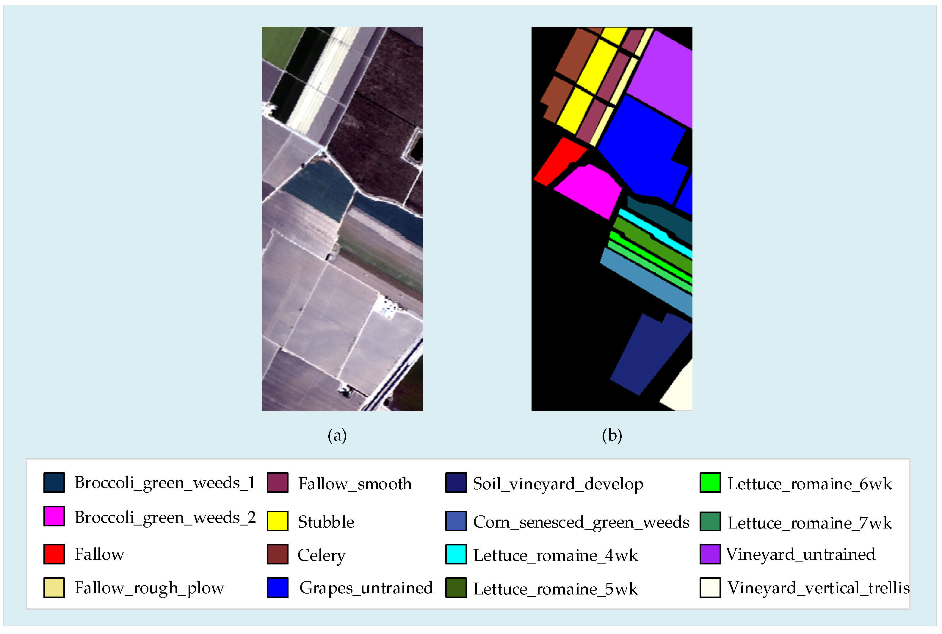
3.1.1. Salinas Dataset

The Salinas dataset is an image of the Salinas Valley in California, USA, collected by an airborne visible infrared imaging spectrometer (AVIRIS), which consists of 512 × 217 pixels, and the spatial resolution is 3.7 m. This dataset has 224 spectral bands originally. In experiments, we used 204 bands after discarding the 108th–112th, 154–167th, and 224th bands because of the water absorption phenomenon. The pseudo-colour image and the ground truth classification map of Salinas are shown in Figure 2.

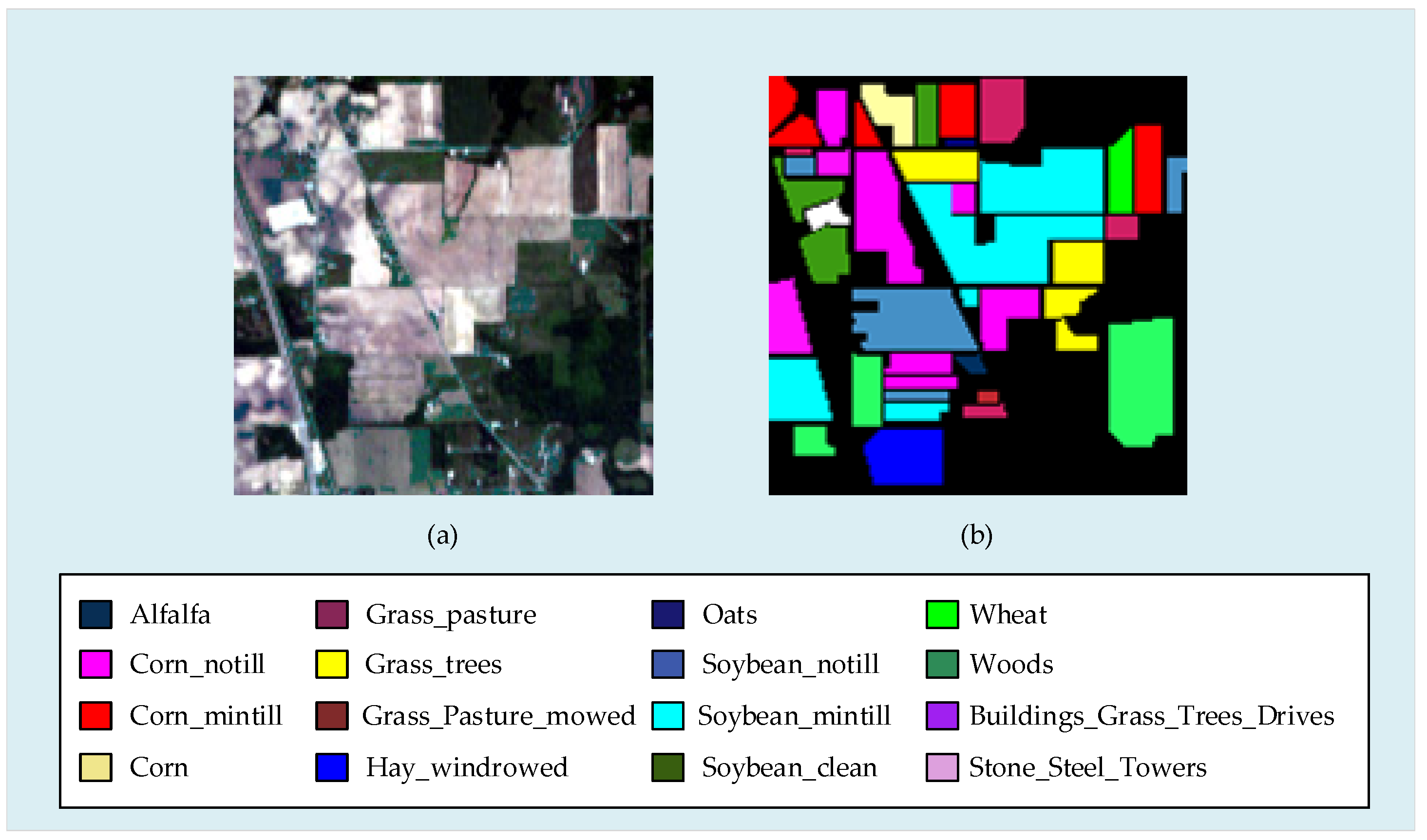
3.1.2. Indian Pines Dataset

Indian Pines is the earliest dataset used for hyperspectral image classification, collected by AVIRIS in Indiana, USA. This dataset consists of 145 × 145 pixels, and the spatial resolution is 20 m. It has 220 spectral bands originally. In the experiments, we used 200 bands after discarding the 104th–180th, 150th–163rd, and 220th bands because of the water absorption phenomenon. The pseudo-colour image and the ground truth classification map of Indian Pines are shown in Figure 3.

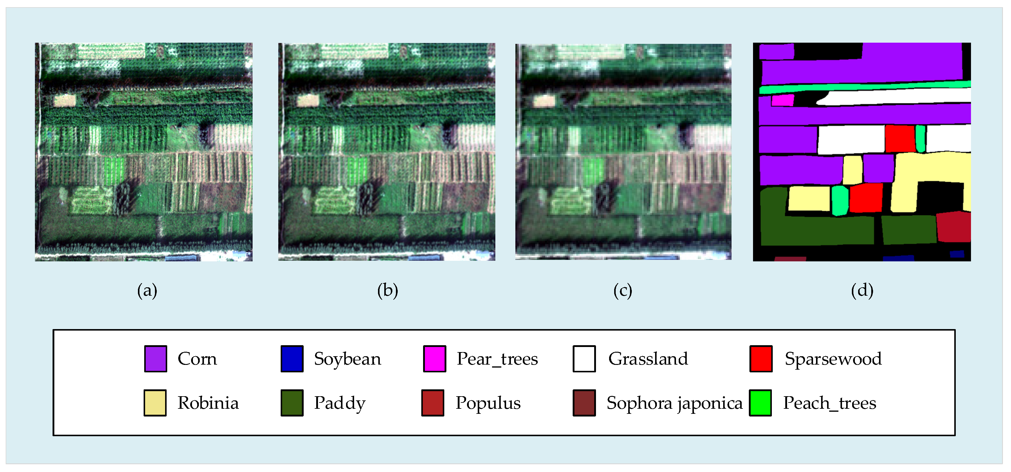
3.1.3. Xiong’an Dataset

Xiong’an is collected in New District, Hebei Province, China by an airborne multi-modular imaging spectrometer (AMMIS), a next-generation Chinese airborne hyperspectral imager. Funded by the China High-Resolution Earth Observation Project, AMMIS was designed and manufactured by the Shanghai Institute of Technical Physics, Chinese Academy of Sciences. This dataset consists of 512 × 512 pixels and 250 spectral bands, the wavelength range is 0.4–1.0 $\mathsf{\mu }\mathrm{m}$, and the spatial resolution is 0.5 m [59,60,61,62,63]. The pseudo-colour image and the ground truth classification map of Xiong’an are shown in Figure 4.

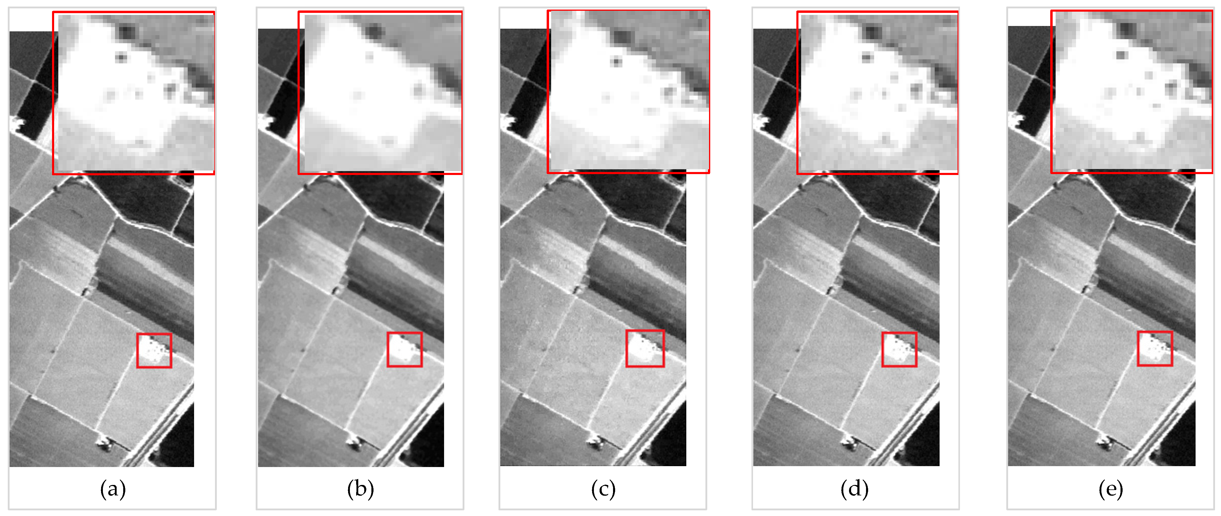
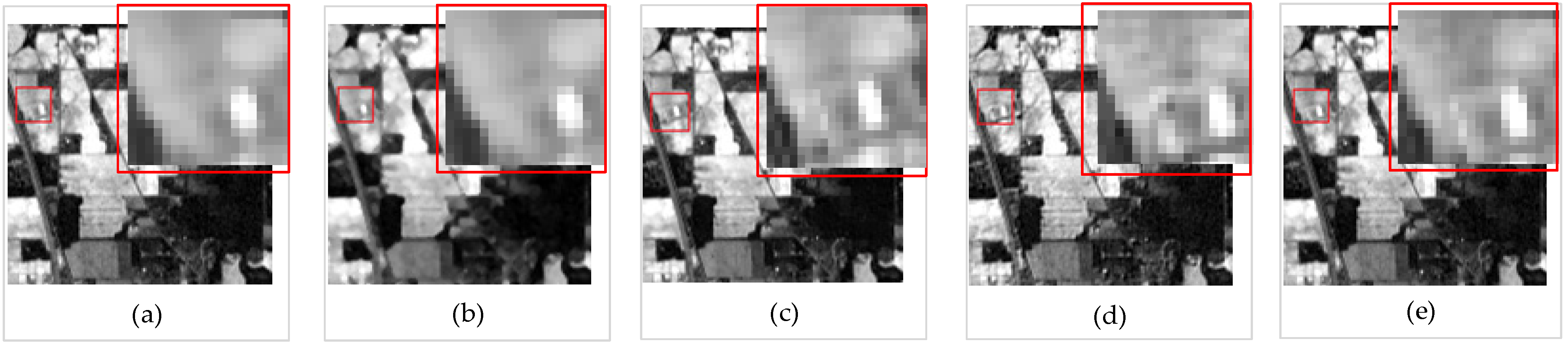
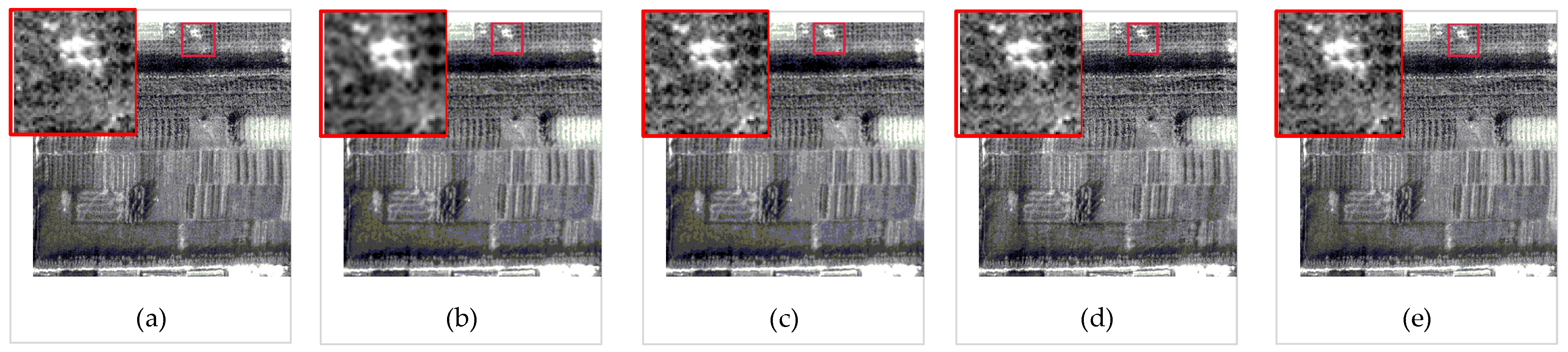
3.2. Experiments on Noise Estimation

The denoised results of KMNF-NE, SSDC, and MNEM were compared, and the MPSNR, MSSIM, and MSAD values on the Salinas, Indian Pines, and Xiong’an datasets are shown in

Table 2. Mean peak signal-to-noise ratio (MPSNR), mean structure similarity (MSSIM) and mean spectral angle distance (MSAD) of different methods on Salinas, Indian Pines, and Xiong’an datasets.

Method	MPSNR	MSSIM	MSAD
Salinas
KMNF-NE	38.43	0.9889	2.3579
SSDC	33.73	0.9377	8.1005
MNEM-Order	26.97	0.9734	2.3828
MNEM-Ratio	43.69	0.9985	0.4701
Indian Pines
KMNF-NE	29.78	0.9487	2.1644
SSDC	26.47	0.8793	6.0796
MNEM-Order	46.29	0.9794	0.1983
MNEM-Ratio	29.76	0.9519	0.5402
Xiong’an
KMNF-NE	33.58	0.9785	2.0654
SSDC	37.86	0.9864	0.8181
MNEM-Order	43.71	0.9787	0.5339
MNEM-Ratio	36.96	0.9907	1.3098

. To visualize the denoised results, we show the denoise results of band 5 in the Salinas dataset, band 187 in the Indian Pines dataset, and band 15 in the Xiong’an dataset in Figure 5, Figure 6 and Figure 7.

In this section, experiments were conducted to assess the noise estimation performance of MENM. As mentioned above, the larger the values of MPSNR and MSSIM and the smaller the value of MSAD, the better the denoised results. Experimental results in this section show that MNEM is more effective, more robust, and retains more details and edge features than KMNF-NE and SSDC. Therefore, we adopt MNEM as the noise estimation method during KMNF for OP-KMNF.

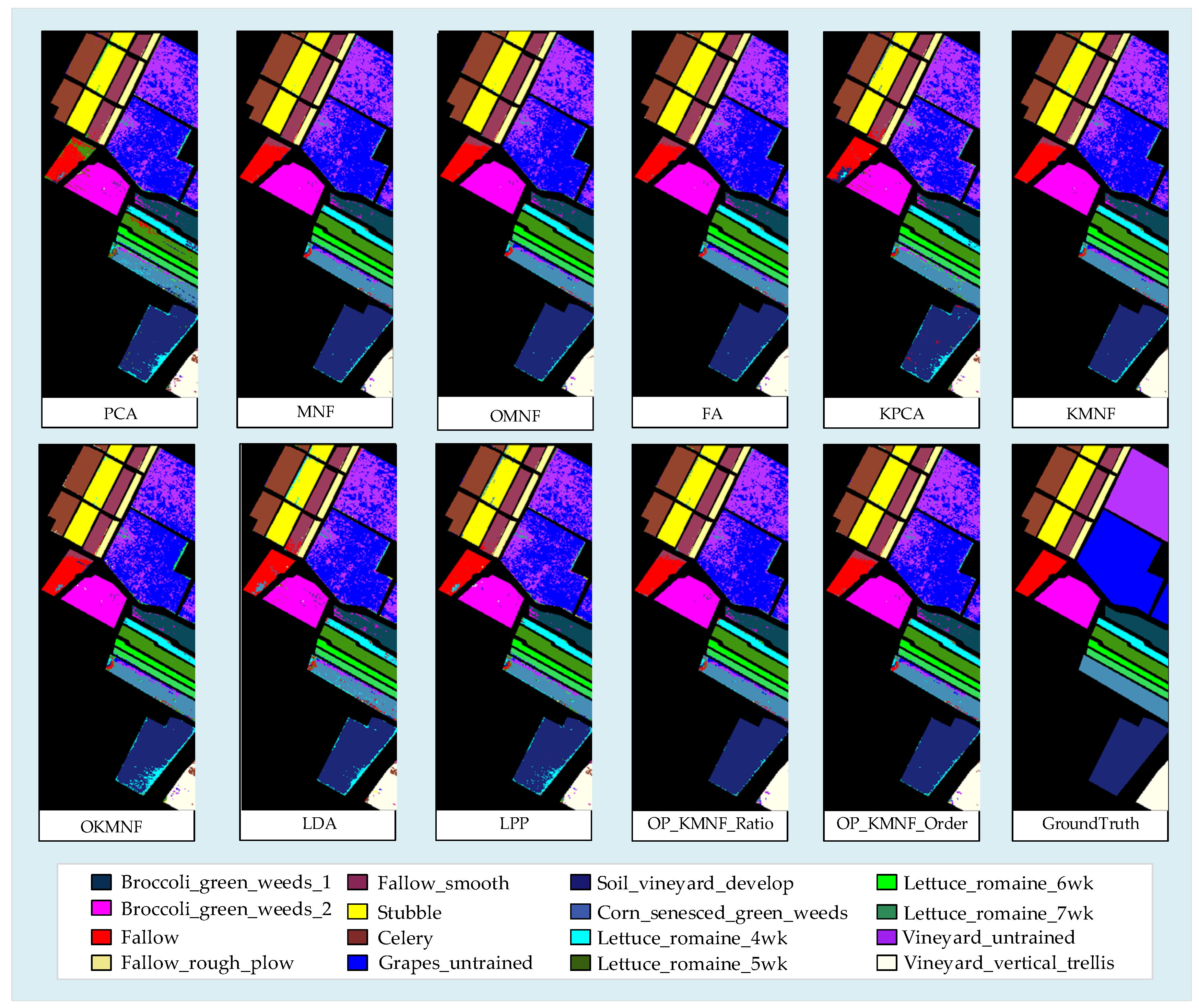
3.3. Experiments on OP-KMNF

The numbers of samples and training samples of the Salinas, Indian Pines, and Xiong’an datasets are listed in

Table 3. Samples and training samples used for the Salinas and Indian Pines datasets.

Classes	Salinas		Classes	Indian Pines
	Samples	Training		Samples	Training
Broccoli_green_weeds_1	2009	502	Alfalfa	46	12
Broccoli_green_weeds_2	3726	932	Corn_notill	1428	357
Fallow	1976	494	Corn_mintill	830	208
Fallow_rough_plow	1394	349	Corn	237	59
Fallow_smooth	2678	670	Grass_pasture	483	121
Stubble	3959	990	Grass_trees	730	183
Celery	3579	895	Grass_pasture_mowed	28	7
Grapes_untrained	11,271	2818	Hay_windrowed	478	120
Soil_vineyard_develop	6203	1551	Oats	20	5
Corn_senesced_green_weeds	3278	820	Soybean_notill	972	243
Lettuce_romaine_4wk	1068	267	Soybean_mintill	2455	614
Lettuce_romaine_5wk	1927	482	Soybean_clean	593	148
Lettuce_romaine_6wk	916	229	Wheat	205	51
Lettuce_romaine_7wk	1070	268	Woods	1265	316
Vineyard_untrained	7268	1817	Buildings_Grass_Trees_Drives	386	97
Vineyard_vertical_trellis	1807	452	Stone_Steel_Towers	93	23

and

Table 4. Samples and training samples used for the Xiong’an dataset.

Classes	Samples	Training
Corn	84,496	21,124
Soybean	10,562	2641
Pear_trees	1303	326
Grassland	27,703	6926
Sparsewood	9292	2323
Robinia	25,761	6440
Paddy	30,029	7507
Populus	5534	1384
Sophora japonica	811	203
Peach_trees	1498	375

. The average accuracies of different DR methods for SVM classification on the Salinas, Indian Pines, and Xiong’an datasets are shown in

Table 5. The average accuracies of support vector machine (SVM) classification in the Salinas, Indian Pines, and Xiong’an datasets after different dimensionality reduction (DR) methods. All the results are percentages.

Salinas
Number of Features	3	4	5	15	25	35	45	55	65
PCA	82.04 $\pm$ 2.13	85.07 $\pm$ 1.50	86.53 $\pm$0.95	90.54 $\pm$1.71	90.93 $\pm$1.55	90.85 $\pm$1.71	91.02 $\pm$1.75	91.23 $\pm$1.57	91.22 $\pm$1.44
MNF	88.42 $\pm$ 1.44	89.15 $\pm$ 1.64	89.22 $\pm$ 1.44	92.30 $\pm$ 0.97	92.80 ± 1.22	92.74 $\pm$ 1.62	92.59 $\pm$ 1.65	92.53 ± 1.59	92.40 $\pm$ 1.69
OMNF	88.55 ± 1.30	89.27 $\pm$ 1.55	89.31 $\pm$ 1.31	92.30 $\pm$ 1.17	92.78 $\pm$ 1.30	92.74 $\pm$ 1.60	92.54 $\pm$ 1.66	92.42 $\pm$ 1.79	92.29 $\pm$ 1.85
FA	85.87 $\pm$ 0.21	89.04 $\pm$ 1.58	89.02 $\pm$ 1.63	91.66 $\pm$ 1.65	92.15 $\pm$ 1.78	92.01 $\pm$ 2.08	93.12 $\pm$ 1.44	93.80 $\pm$ 0.97	93.76 $\pm$ 0.84
KPCA	86.14 $\pm$ 0.61	88.37 $\pm$ 0.67	88.48 $\pm$ 0.84	90.26 ± 1.61	90.85 $\pm$ 1.75	91.09 $\pm$ 1.87	91.37 $\pm$ 1.84	91.45 $\pm$ 1.96	91.40 $\pm$ 1.95
KMNF	88.42 $\pm$ 1.44	89.15 ± 1.64	89.22 $\pm$ 1.44	92.30 $\pm$ 0.97	92.80 $\pm$ 1.22	92.74 $\pm$ 1.62	92.60 $\pm$ 1.64	92.54 $\pm$ 1.58	92.41 $\pm$ 1.68
OKMNF	87.32 $\pm$ 1.19	88.55 $\pm$ 1.13	88.43 $\pm$ 1.05	92.01 $\pm$ 1.14	92.97 $\pm$ 1.32	93.21 $\pm$ 1.29	93.25 $\pm$ 1.31	93.59 $\pm$ 1.46	93.66 $\pm$ 1.26
LDA	86.27 $\pm$ 1.84	86.72 $\pm$ 1.47	88.61 $\pm$ 1.85	90.79 $\pm$ 2.12	91.46 $\pm$ 1.96	91.37 $\pm$ 1.88	91.35 $\pm$ 1.83	91.49 $\pm$ 1.51	91.48 ± 1.53
LPP	86.30 $\pm$ 0.96	88.86 $\pm$ 1.43	89.22 $\pm$ 1.43	91.36 $\pm$ 2.28	91.94 $\pm$ 1.90	92.05 $\pm$ 2.00	91.91 $\pm$ 1.88	91.88 $\pm$ 1.81	91.85 $\pm$ 2.04
OP-KMNF-Ratio	87.25 $\pm$ 0.46	91.12 $\pm$1.62	91.64 $\pm$1.70	93.92 $\pm$1.16	94.25 $\pm$1.20	94.50 $\pm$1.36	94.63 $\pm$1.59	94.61 $\pm$1.72	94.69 $\pm$1.81
OP-KMNF-Order	89.86 $\pm$ 0.45	90.80 $\pm$ 1.66	90.66 $\pm$ 1.44	93.27 $\pm$ 0.98	94.02 $\pm$ 1.21	94.36 $\pm$ 1.62	94.23 $\pm$ 1.64	94.12 $\pm$ 1.59	94.09 $\pm$ 1.67
Indian Pines
Number of Features	3	4	5	6	7	8		9
PCA	36.45 $\pm$ 3.49	43.97 $\pm$ 3.43	44.92 $\pm$ 1.79	44.83 $\pm$ 1.46	49.87 $\pm$ 1.05	52.91 $\pm$ 2.93		53.65 $\pm$ 1.98
MNF	55.33 $\pm$ 0.04	57.84 $\pm$ 1.32	58.88 $\pm$ 0.79	59.66 $\pm$ 2.25	60.97 $\pm$ 0.85	61.85 $\pm$ 1.38		60.94 $\pm$ 2.20
OMNF	54.49 $\pm$ 0.59	57.06 $\pm$ 1.40	58.40 $\pm$ 1.06	59.38 $\pm$ 2.59	60.97 $\pm$ 1.70	61.83 $\pm$ 1.21		60.94 $\pm$ 1.91
FA	47.14 $\pm$ 0.52	54.49 $\pm$ 0.94	55.94 $\pm$ 0.59	57.40 $\pm$ 3.57	59.22 $\pm$ 2.67	61.41 $\pm$ 0.12		61.13 $\pm$ 1.54
KPCA	36.36 $\pm$ 0.63	39.69 $\pm$ 0.61	41.55 $\pm$ 0.69	43.85 $\pm$ 0.76	47.01 $\pm$ 0.23	47.60 $\pm$ 0.12		52.86 $\pm$ 0.42
KMNF	52.25 $\pm$ 1.18	55.05 $\pm$ 0.70	55.83 $\pm$ 1.38	58.54 $\pm$ 0.43	56.87 $\pm$0.09	58.38 $\pm$ 0.04		60.90 $\pm$ 2.30
OKMNF	32.67 $\pm$ 0.42	43.99 $\pm$ 1.79	43.51 $\pm$ 1.75	46.30 $\pm$ 0.31	49.55 $\pm$ 1.68	51.30 $\pm$ 2.17		54.47 $\pm$ 2.10
LDA	31.92 $\pm$ 0.98	39.32 $\pm$ 0.12	49.51 $\pm$ 1.83	52.44 $\pm$ 0.28	54.86 $\pm$ 1.15	54.90 $\pm$ 0.60		55.57 $\pm$ 1.17
LPP	36.55 $\pm$ 0.68	42.49 $\pm$ 0.26	44.94 $\pm$ 1.32	55.86 $\pm$ 5.62	54.76 $\pm$ 3.73	58.20 $\pm$ 2.78		59.26 $\pm$ 0.62
OP-KMNF-Ratio	56.00 $\pm$ 0.19	58.54 $\pm$ 0.20	59.54 $\pm$0.64	55.99 $\pm$ 0.35	56.54 $\pm$ 1.36	60.80 $\pm$ 1.04		60.71 $\pm$ 0.87
OP-KMNF-Order	53.72 $\pm$ 0.20	57.25 $\pm$ 1.04	56.88 $\pm$ 0.08	61.50 $\pm$ 1.47	61.79 $\pm$ 0.52	61.90 $\pm$ 0.29		62.98 $\pm$ 1.27
Xiong’an
Number of Features	3	4	5	6	7	8		9
PCA	31.05 $\pm$ 1.78	31.70 $\pm$ 1.91	36.03 $\pm$ 2.64	36.82 $\pm$ 2.97	37.00 $\pm$ 2.75	44.25 $\pm$ 3.04		46.36 $\pm$ 1.94
MNF	38.12 $\pm$ 0.45	51.98 $\pm$ 1.37	55.93 $\pm$ 2.62	60.17 $\pm$ 1.69	62.83 $\pm$ 0.85	64.11 $\pm$ 1.95		67.03 $\pm$ 0.90
OMNF	38.15 $\pm$ 0.51	53.39 ± 1.47	58.54 $\pm$ 2.63	60.01 $\pm$ 1.77	62.94 $\pm$ 0.81	63.98 $\pm$ 1.98		66.91 $\pm$ 0.88
FA	40.39 $\pm$ 2.56	51.82 $\pm$ 1.94	54.59 $\pm$ 2.14	57.03 $\pm$ 1.55	57.88 $\pm$ 1.24	58.74 $\pm$ 0.97		59.54 $\pm$ 1.14
KPCA	29.60 $\pm$ 2.54	34.12 $\pm$ 1.40	34.75 $\pm$ 1.90	34.83 $\pm$ 1.64	35.58 $\pm$ 1.71	37.97 $\pm$ 1.77		38.34 $\pm$ 1.65
KMNF	43.82 $\pm$ 2.30	51.27 $\pm$ 2.16	54.37 $\pm$ 2.40	58.61 $\pm$ 1.56	61.71 $\pm$ 2.15	60.57 $\pm$ 1.87		63.38 $\pm$ 2.11
OKMNF	39.42 $\pm$ 1.74	53.34 $\pm$ 1.32	58.98 $\pm$ 1.48	59.61 $\pm$ 1.66	61.41 $\pm$ 2.17	63.18 $\pm$ 0.85		65.71 $\pm$ 0.83
LDA	37.57 $\pm$ 2.35	40.93 $\pm$ 3.65	42.25 $\pm$ 3.21	43.00 $\pm$ 1.11	44.94 $\pm$ 2.31	49.51 $\pm$ 2.18		55.88 $\pm$ 2.19
LPP	30.03 $\pm$ 1.13	41.48 $\pm$ 3.86	46.29 $\pm$ 3.96	47.75 $\pm$ 4.06	52.96 $\pm$ 3.69	53.21 $\pm$ 2.32		54.35 $\pm$ 2.05
OP-KMNF-Ratio	43.99 $\pm$ 2.02	54.03 $\pm$ 1.69	58.47 $\pm$ 1.46	61.42 $\pm$ 0.99	64.42 $\pm$ 1.30	68.03 $\pm$ 0.52		70.14 $\pm$ 0.23
OP-KMNF-Order	48.36 $\pm$ 0.98	54.32 $\pm$ 1.20	59.53 $\pm$ 2.95	61.73 $\pm$ 0.75	62.38 $\pm$ 1.42	65.60 $\pm$ 2.16		67.35 $\pm$ 1.97

. Taking the feature extracted by each method in the Xiong’an dataset (number of features = 9) as an example, the statistics on the classification accuracies of each class are given in

Table 6. The class accuracies of SVM classification on Xiong’an with number of features = 9. All the results are percentages.

Classes	Corn	Soybean	Pear_Trees	Grassland	Sparsewood	Robinia	Paddy	Populus	Sophora Japonica	Peach_Trees
PCA	69.72	28.10	51.11	39.88	8.09	69.22	63.74	13.28	29.10	91.32
MNF	79.33	88.54	77.13	65.15	47.18	78.34	75.48	23.49	48.46	87.25
OMNF	79.25	88.62	76.90	64.94	46.86	78.37	75.39	23.40	48.09	87.25
FA	74.98	76.97	73.98	46.20	29.60	75.40	66.89	25.03	36.00	90.39
KPCA	69.17	19.63	37.68	33.76	3.95	69.06	50.52	6.27	0.00	93.32
KMNF	77.40	83.59	77.21	61.32	44.64	77.21	59.73	31.91	31.44	89.32
OKMNF	76.54	83.13	74.52	52.80	40.17	83.32	77.75	32.62	47.84	88.38
LDA	73.54	73.69	70.22	43.43	22.31	70.98	72.47	29.80	12.08	90.25
LPP	71.13	63.98	73.98	46.16	30.28	68.72	67.16	32.06	0.00	89.99
OP-KMNF (Ratio)	78.17	87.67	75.98	52.60	44.19	80.54	81.14	42.84	69.30	88.99
1Rank 2Improve	3 −1.16	3 −0.87	4 −1.23	5 −12.55	4 −2.99	2 −2.77	1 +3.39	1 +10.22	1 +20.84	7 −4.33
OP-KMNF (Order)	79.42	84.65	76.82	45.35	44.07	83.42	76.39	43.02	48.71	91.66
Rank Improve	1 +0.09	3 −3.89	4 −0.39	7 −19.80	5 −3.11	1 +0.10	2 −1.36	1 +10.40	1 +0.25	2 −1.66

¹ The rank of OP-KMNF in class accuracy. ² The improvement of OP-KMNF compared with the method that has the best class accuracy.

. In order to visualize the classification results, the SVM classification results of the Indian Pines, Salinas, and Xiong’an datasets after different DR methods (number of features = 5) are shown in Figure 8, Figure 9 and Figure 10.

In this section, SVM is used as the classification algorithm, and the average accuracy is used to assess the results. Experimental results, obtained using multiple hyperspectral datasets (including the Indian Pines dataset, Salinas dataset, and Xiong’an dataset), show that OP-KMNF overperforms other traditional DR methods (including LDA, PCA, MNF, OMNF, FA, KPCA, KMNF, OKMNF, and LPP) in terms of the average classification accuracy. The improvements of OP-KMNF in terms of the average accuracy on the Salinas, Indian Pines, and Xiong’an datasets were 2.33%, 1.85%, and 4.54%, respectively, and, compared with KMNF, the improvements were 2.42%, 4.92%, and 7.64%. Taking the feature extracted by each method in the Xiong’an dataset (number of features = 9) as an example, the classification accuracy of each class was assessed. In the classification of Corn, Robinia, Populus and Sophora japonica, OP-KMNF showed a significant improvement compared with the other methods.

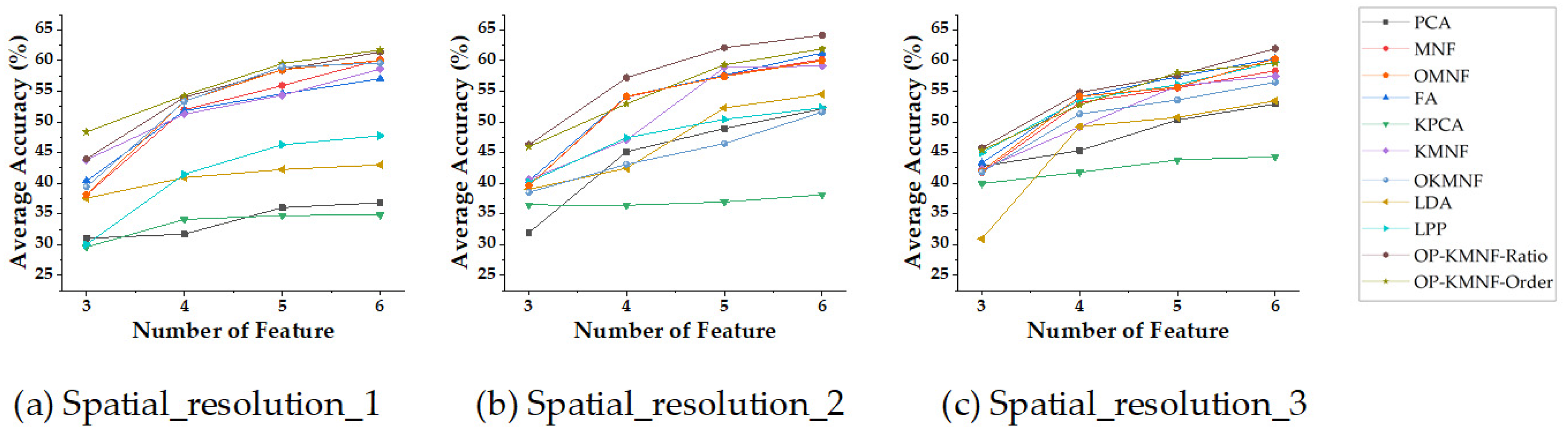
3.4. Adaptability of OP-KMNF to Hyperspectral Images with Different Spatial Resolutions

HSIs with different spatial resolutions are obtained after pixel merging on the Xiong’an dataset. We treat the Xiong’an dataset as Spatial_resolution_1, and for each band, four adjacent pixels are averaged to obtain Spatial_resolution_2, and eight adjacent pixels are averaged to obtain Spatial_resolution_3. The spatial resolution of Spatial_resolution_1 is 0.5 m, the spatial resolution of Spatial_resolution_2 is 1 m, and the spatial resolution of Spatial_resolution_3 is 2 m. The pseudo-colour images and the ground truth classification map are shown in Figure 11.

The numbers of samples and training samples used in the Xiong’an dataset with different spatial resolutions are listed in

Table 7. Samples and training samples used in Xiong’an dataset with different spatial resolutions.

Classes	Spatial_Resolution_1 (0.5 m)		Spatial_Resolution_2 (1 m)		Spatial_Resolution_3 (2 m)
	Samples	Training	Samples	Training	Samples	Training
Corn	84,496	21,124	20,728	5182	4925	1231
Soybean	10,562	2641	2474	618	523	130
Pear_trees	1303	326	312	78	71	18
Grassland	27,703	6926	6734	1683	1583	396
Sparsewood	9292	2323	2254	563	534	133
Robinia	25,761	6440	6274	1568	1508	377
Paddy	30,029	7507	7364	1841	1761	440
Populus	5534	1384	1345	336	318	80
Sophora japonica	811	203	182	45	36	9
Peach_trees	1498	375	348	87	73	18

. The average accuracies of different DR methods for SVM classification are shown in Figure 12.

In this section, experiments are conducted to verify the adaptability of OP-KMNF to HSIs with different spatial resolutions. For experiments on Spatial_resolution_1, Spatial_resolution_2, and Spatial_resolution_3, the OP-KMNF showed better performance compared with some other DR methods (including LDA, PCA, MNF, OMNF, FA, KPCA, KMNF, OKMNF, and LPP).

3.5. Adaptability of OP-KMNF to Hyperspectral Images with Different Spectral Resolutions

HSIs with different spectral resolutions were obtained after band merging on the Xiong’an dataset. We treat the Xiong’an dataset as Spectral_resolution_1, and for each pixel, two adjacent bands are averaged to obtain Spectral_resolution_2, and four adjacent bands are averaged to obtain Spectral_resolution_3. The spectral resolution of Spectral_resolution_1 is 2.4 nm, the spectral resolution of Spectral_resolution_2 is 4.8 nm, and the spectral resolution of Spectral_resolution_3 is 9.6 nm. The pseudo-colour images and the ground truth classification map are shown in Figure 13.

The numbers of samples and training samples used in the Xiong’an dataset with different spectral resolutions are listed in

Table 8. Samples and training samples used in the Xiong’an with different spectral resolutions.

Classes	Spectral_Resolution_1 (2.4 nm)		Spectral _Resolution_2 (4.8 nm)		Spectral _Resolution_3 (9.6 nm)
	Samples	Training	Samples	Training	Samples	Training
Corn	84,496	21,124	84,496	21,124	84,496	21,124
Soybean	10,562	2641	10,562	2641	10,562	2641
Pear_trees	1303	326	1303	326	1303	326
Grassland	27,703	6926	27,703	6926	27,703	6926
Sparsewood	9292	2323	9292	2323	9292	2323
Robinia	25,761	6440	25,761	6440	25,761	6440
Paddy	30,029	7507	30,029	7507	30,029	7507
Populus	5534	1384	5534	1384	5534	1384
Sophora japonica	811	203	811	203	811	203
Peach_trees	1498	375	1498	375	1498	375

. The average accuracies of different DR methods for SVM classification are shown in Figure 14.

In this section, experiments are conducted to verify the adaptability of OP-KMNF to HSIs with different spectral resolutions. For experiments on Spectral_resolution_1, Spectral_resolution_2, and Spectral_resolution_3, the OP-KMNF showed better performance compared with some other DR methods (including LDA, PCA, MNF, OMNF, FA, KPCA, KMNF, OKMNF, and LPP).

3.6. GPU Implementation of OP-KMNF

Table 9. The runtimes and speedups of OP-KMNF on two different computing systems.

Data Sizes	CPU Runtime	GPU1 Runtime	Speedups1	GPU2 Runtime	Speedups2
OP-KMNF-Order
100 × 100 × 250	307.730 s	20.924 s	14.92×	12.251 s	25.12×
150 × 150 × 250	678.703 s	30.373 s	22.35×	17.352 s	39.11×
200 × 200 × 250	1177.293 s	44.535 s	26.44×	23.923 s	49.21×
250 × 250 × 250	1837.850 s	63.312 s	29.03×	34.143 s	53.83×
300 × 300 × 250	2627.564 s	85.893 s	30.59×	45.275 s	58.04×
350 × 350 × 250	3586.769 s	113.238 s	31.67×	58.944 s	60.85×
400 × 400 × 250	4682.999 s	142.582 s	32.84×	73.232 s	63.95×
OP-KMNF-Ratio
100 × 100 × 250	317.973 s	21.906 s	14.52×	12.511 s	25.42×
150 × 150 × 250	704.654 s	32.255 s	21.85×	18.161 s	38.80×
200 × 200 × 250	1234.365 s	46.222 s	26.71×	24.101 s	51.22×
250 × 250 × 250	1918.372 s	66.053 s	29.04×	34.686 s	55.31×
300 × 300 × 250	2742.355 s	88.857 s	30.86×	46.064 s	59.53×
350 × 350 × 250	3739.979 s	119.276 s	31.36×	59.001 s	63.39×
400 × 400 × 250	4877.802 s	151.954 s	32.10×	75.891 s	64.27×

shows the runtimes and speedups of OP-KMNF before parallel computing and after on two different computing systems with different data volumes. The CPU runtime was tested on computing system No. 1. Taking the processing with the data volume is 400 × 400 $\times$ 250 as an example, we detail the computational costs of OP-KMNF, and the result is shown in

Table 10. The computational costs of OP-KMNF when the data volume is 400 × 400 × 250.

Program × Execution	OP-KMNF-Order			OP-KMNF-Ratio
	CPU Runtime	GPU1 Runtime	GPU2 Runtime	CPU Runtime	GPU1 Runtime	GPU2 Runtime
Data reading	29.342 s	29.342 s	3.365 s	29.342 s	29.342 s	3.365 s
Noise estimation	2300.203 s	82.571 s	61.605 s	2471.537 s	91.206 s	63.606 s
KMNF transformation	2402.198 s	13.804 s	4.292 s	2402.198 s	13.804 s	4.292 s
Output	31.525 s	31.525 s	0.202 s	31.525 s	31.525 s	0.202 s

.

In this section, experiments were conducted to compare the time consumption before and after parallel computing in OP-KMNF with identical data volumes on two different computing systems. The experimental results show that OP-KMNF implemented in parallel on GPU leads to a significant improvement in efficiency. For experiments on a data volume of 400 $\times$ 400 $\times$ 250, the improvements of OP-KMNF-Order and OP-KMNF-Ratio sped up by 63.95× and 64.27×, respectively. For the computational costs of OP-KMNF with a data volume of 400 $\times$ 400 $\times$ 250, it can be seen that, in computing system No. 1, the execution efficiency of OP-KMNF-Order and OP-KMNF-Ratio in noise estimation sped up by 27.86× and 27.10× and that, in computing system No. 2, they sped up by 37.34× and 38.86×. For KMNF transformation, the execution efficiency sped up by 174.02× in computing system No. 1 and 559.69× in computing system No. 2.

4. Discussion

In this section, we discuss the performance of MNEM, OP-KMNF, and parallel computing on GPU that are proposed in this paper. The results were given in Section 3.

We conducted experiments to assess the noise estimation performance of MENM, and the results demonstrate that MNEM is more effective, more robust, and retains more details and edge features than KMNF-NE. From the experimental results of the Salinas dataset (spatial resolution: 3.7 m), Indian Pines dataset (spatial resolution: 20 m), and Xiong’an dataset (spatial resolution: 0.5 m), the improvements of MENM in MPSNR, MSSIM, and MASD were greatest for the Indian Pines dataset, which shows that MENM had better performance than KMNF-NE and SSDC on a dataset with limited spatial resolution and lots of mixed pixels. As mentioned above, noise estimation is a crucial component in KMNF, so we adopted MNEM for noise estimation during KMNF for OP-KMNF.

We validated the performance of DR methods in terms of SVM, and the average accuracy was used to assess the results. Experimental results obtained using three real hyperspectral datasets (the Indian Pines dataset, Salinas dataset, and Xiong’an dataset) showed that, (1) compared with other DR methods (including LDA, PCA, MNF, OMNF, FA, KPCA, KMNF, OKMNF, and LPP), OP-KMNF led to significant improvements in terms of the average classification accuracy; (2) it is not the case that the more features are extracted, the higher the classification accuracy will be, so the number of features should be selected to achieve the highest classification accuracy; (3) in practice, FA can be used as a dimensionality reduction method, and in many cases, it has better performance than MNF and KMNF; and (4) the experimental results prove the importance of accurate noise estimation for the KMNF algorithm and provide a way to optimize KMNF in the future. Compared to the other nine DR algorithms under the same experimental conditions, OP-KMNF handles the non-linear features well and performs better in subsequent classification processing.

To verify the adaptability of OP-KMNF to HSIs with different spatial resolutions, we obtained HSIs with different spatial resolutions by using pixel merging on the Xiong’an dataset. The spatial resolution of Spatial_resolution_1, Spatial_resolution_2, and Spatial_resolution_3 was 0.5 m, 1 m, and 2 m, respectively. Experimental results obtained using these images showed that, (1) compared with other DR methods (including LDA, PCA, MNF, OMNF, FA, KPCA, KMNF, OKMNF, and LPP), OP-KMNF led to significant improvements in average classification accuracy on HSIs with different spatial resolutions; (2) in most cases, the performance of DR methods (including LDA, PCA, MNF, OMNF, FA, KPCA, KMNF, OKMNF, LPP, and OP-KMNF) in classification was improved with the decrease in spatial resolution; and (3) the MNEM adapts HSIs with different spatial resolutions well during KMNF and, the lower the spatial resolution, the more the performance improvement of OP-KMNF over KMNF.

To verify the adaptability of OP-KMNF to HSIs with different spectral resolutions, we obtained HSIs with different spectral resolutions by using band merging on the Xiong’an dataset; the spectral resolution of Spectral_resolution_1, Spectral_resolution_2, and Spectral_resolution_3 was 2.4 nm, 4.8 nm, and 9.6 nm, respectively. Experimental results obtained using these images showed that, (1) compared with other DR methods (including LDA, PCA, MNF, OMNF, FA, KPCA, KMNF, OKMNF, and LPP), OP-KMNF led to significant improvements in terms of average classification accuracy on HSIs with different spectral resolutions; (2) the performance of LDA and LPP in classification improved with the decrease in spectral resolution, while the performance of KMNF and OKMNF worsened with the decrease in spectral resolution; and (3) the MNEM adapts the HSIs with different spectral resolutions during KMNF well and the lower the spectral resolution, the greater the performance improvement of OP-KMNF over KMNF.

In practice, we need to consider both the performance and the efficiency. We introduced GPU-based parallel computing to improve the execution efficiency of OP-KMNF and compared the time consumption before and after parallel computing under the same data volumes on two different computing systems. The results showed that the implementation in parallel on GPU led to a significant improvement in efficiency. The analysis of the experimental results in Table 9 and Table 10 showed that, (1) the larger the data volume, the more significant the acceleration effect; (2) when the data volume was 400 $\times$ 400 $\times$ 251, the execution efficiency sped up by about 60× compared to the CPU implementation; and (3) with the development of parallel systems, the execution efficiency of the algorithm is further improved.

From the experimental results, we can see that the MNEM-Order and MNEM-Ratio have different adaptability on different datasets. For the experimental results on the Salinas dataset, the MNEM-Ratio shows better noise estimation performance, while on the Indian Pines and Xiong’an datasets, MNEM-Order shows better performance. In most cases, OP-KMNF-Ratio shows better performance on the Salinas dataset in terms of the average classification accuracy, while OP-KMNF-Order shows better performance when the feature number is 3. Similar experimental results have also appeared in the Indian Pines dataset and Xiong’an dataset. The reason for this phenomenon is still incompletely understood.

To further analyse the causes of this phenomenon, the PSNR and SSIM values of each band on the Salinas, Indian Pines, and Xiong’an datasets are shown in Figure 15 and Figure 16. It can be seen that each noise estimation method has different adaptability to different bands. For KMNF transformation, it is not the case that the more features are extracted, the higher the classification accuracy will be; the noise fraction matrix of the HSI is processed as a whole during the KMNF transformation, and the impact of the noise estimation results of each band on the final results has not been quantitatively assessed. All of these factors have an impact on the final results. In future work, we will perform more in-depth research to explain this phenomenon.

5. Conclusions

The MNEM proposed in this paper can estimate the noise of HSI more effectively, is more robust, retains more details and edge features than KMNF-NE, and further optimizes the DR performance of KMNF in terms of classification. In consideration of the computational cost, we introduce GPU-based parallel computing to OP-KMNF. Experimental results show that this algorithm handles non-linear features well and perfectly adapts HSIs with different spatial resolutions and spectral resolutions. Additionally, it is superior to other commonly used DR algorithms in terms of classification. The experiments on two different computing systems proved that the execution efficiency is further improved with parallel system development, which clarifies the real-time dimensionality reduction for HSI. In the future, the performance of OP-KMNF in other applications (e.g., anomaly detection), and the implementation of its real-time algorithm will be studied.

References

1. Keshava, N.; Mustard, J.F. Spectral unmixing. IEEE Signal Process. Mag. 2002, 19, 44–57. [Google Scholar] [CrossRef]
2. Gao, L.; Du, Q.; Zhang, B.; Yang, W.; Wu, Y. A Comparative study on linear regression-based noise estimation for hyperspectral imagery. IEEE J. Sel. Top. Appl. Earth Obs. Remote Sens. 2013, 6, 488–498. [Google Scholar] [CrossRef] [Green Version]
3. Jia, J.; Wang, Y.; Chen, J.; Guo, R.; Shu, R.; Wang, J. Status and application of advanced airborne hyperspectral imaging technology: A review. Infrared Phys. Technol. 2020, 104, 103115. [Google Scholar] [CrossRef]
4. Bruce, L.; Koger, C.; Li, J. Dimensionality reduction of hyperspectral data using discrete wavelet transform feature extraction. IEEE Trans. Geosci. Remote Sens. 2002, 40, 2331–2338. [Google Scholar] [CrossRef]
5. Zhao, B.; Gao, L.; Liao, W.; Zhang, B. A new kernel method for hyperspectral image feature extraction. Geospat. Inf. Sci. 2017, 20, 309–318. [Google Scholar] [CrossRef] [Green Version]
6. Zhou, Y.; Peng, J.; Chen, C.L.P. Dimension Reduction Using Spatial and Spectral Regularized Local Discriminant Embedding for Hyperspectral Image Classification. IEEE Trans. Geosci. Remote Sens. 2015, 53, 1082–1095. [Google Scholar] [CrossRef]
7. Hughes, G. On the mean accuracy of statistical pattern recognizers. IEEE Trans. Inf. Theory 1968, 14, 55–63. [Google Scholar] [CrossRef] [Green Version]
8. Liang, L.; Xia, Y.; Xun, L.; Yan, Q.; Zhang, D. Class-Probability Based Semi-Supervised Dimensionality Reduction for Hyperspectral Images. In Proceedings of the 2018 IEEE 9th International Conference on Software Engineering and Service Science (ICSESS), Beijing, China, 23–25 September 2018; pp. 460–463. [Google Scholar]
9. Feng, J.; Jiao, L.; Liu, F.; Sun, T.; Zhang, X. Mutual-information-based semi-supervised hyperspectral band selection with high discrimination, high information, and low redundancy. IEEE Trans. Geosci. Remote Sens. 2014, 53, 2956–2969. [Google Scholar] [CrossRef]
10. Chen, W.; Yang, Z.; Cao, F.; Yan, Y.; Wang, M.; Qing, C.; Cheng, Y. Dimensionality reduction based on determinantal point process and singular spectrum analysis for hyperspectral images. IET Image Process. 2019, 13, 299–306. [Google Scholar] [CrossRef] [Green Version]
11. Sun, W.; Du, Q. Hyperspectral band selection: A review. IEEE Geosci. Remote Sens. Mag. 2019, 7, 118–139. [Google Scholar] [CrossRef]
12. Chang, C.-I.; Du, Q.; Sun, T.-L.; Althouse, M. A joint band prioritization and band-decorrelation approach to band selection for hyperspectral image classification. IEEE Trans. Geosci. Remote Sens. 1999, 37, 2631–2641. [Google Scholar] [CrossRef] [Green Version]
13. Bajcsy, P.; Groves, P. Methodology for hyperspectral band selection. Photogramm. Eng. Remote Sens. 2004, 70, 793–802. [Google Scholar] [CrossRef]
14. Yang, H.; Du, Q.; Su, H.; Sheng, Y. An efficient method for supervised hyperspectral band selection. IEEE Geosci. Remote Sens. Lett. 2010, 8, 138–142. [Google Scholar] [CrossRef]
15. Keshava, N. Distance metrics and band selection in hyperspectral processing with applications to material identification and spectral libraries. IEEE Trans. Geosci. Remote Sens. 2004, 42, 1552–1565. [Google Scholar] [CrossRef]
16. Su, H.; Du, Q.; Chen, G.; Du, P. Optimized hyperspectral band selection using particle swarm optimization. IEEE J. Sel. Top. Appl. Earth Obs. Remote Sens. 2014, 7, 2659–2670. [Google Scholar] [CrossRef]
17. Martínez-Usómartinez-Uso, A.; Pla, F.; Sotoca, J.M.; García-Sevilla, P. Clustering-based hyperspectral band selection using information measures. IEEE Trans. Geosci. Remote Sens. 2007, 45, 4158–4171. [Google Scholar] [CrossRef]
18. Cariou, C.; Chehdi, K.; Le Moan, S. BandClust: An unsupervised band reduction method for hyperspectral remote sensing. IEEE Geosci. Remote Sens. Lett. 2010, 8, 565–569. [Google Scholar] [CrossRef]
19. Zhang, M.; Ma, J.; Gong, M. Unsupervised hyperspectral band selection by fuzzy clustering with particle swarm optimization. IEEE Geosci. Remote Sens. Lett. 2017, 14, 773–777. [Google Scholar] [CrossRef]
20. Li, J.-M.; Qian, Y.-T. Clustering-based hyperspectral band selection using sparse nonnegative matrix factorization. J. Zhejiang Univ. Sci. C 2011, 12, 542–549. [Google Scholar] [CrossRef]
21. Li, S.; Qi, H. Sparse Representation-Based Band Selection for Hyperspectral Images. In Proceedings of the 18th IEEE International Conference on Image Processing, Brussels, Belgium, 11–14 September 2011; pp. 2693–2696. [Google Scholar] [CrossRef]
22. Sun, W.; Zhang, L.; Du, B.; Li, W.; Lai, Y.M. Band selection using improved sparse subspace clustering for hyperspectral imagery classification. IEEE J. Sel. Top. Appl. Earth Obs. Remote Sens. 2015, 8, 2784–2797. [Google Scholar] [CrossRef]
23. Yin, J.; Wang, Y.; Zhao, Z. Optimal Band Selection for Hyperspectral Image Classification Based on Inter-Class Separability. In Proceedings of the 2010 Symposium on Photonics and Optoelectronics, Chengdu, China, 19–21 June 2010; pp. 1–4. [Google Scholar] [CrossRef]
24. Sildomar, T.-M.; Yukio, K. A Particle Swarm Optimization-Based Approach for Hyperspectral Band Selection. In Proceedings of the 2007 IEEE Congress on Evolutionary Computation, Singapore, 25–28 September 2007; pp. 3335–3340. [Google Scholar] [CrossRef]
25. Wang, Q.; Lin, J.; Yuan, Y. Salient band selection for hyperspectral image classification via manifold ranking. IEEE Trans. Neural Netw. Learn. Syst. 2016, 27, 1279–1289. [Google Scholar] [CrossRef] [PubMed]
26. Gao, L.; Zhao, B.; Jia, X.; Liao, W.; Zhang, B. Optimized kernel minimum noise fraction transformation for hyperspectral image classification. Remote Sens. 2017, 9, 548. [Google Scholar] [CrossRef] [Green Version]
27. Berry, M.; Browne, M.; Langville, A.N.; Pauca, V.P.; Plemmons, R.J. Algorithms and applications for approximate nonnegative matrix factorization. Comput. Stat. Data Anal. 2007, 52, 155–173. [Google Scholar] [CrossRef] [Green Version]
28. Casalino, G.; Gillis, N. Sequential dimensionality reduction for extracting localized features. Pattern Recognit. 2017, 63, 15–29. [Google Scholar] [CrossRef] [Green Version]
29. Bandos, T.V.; Bruzzone, L.; Camps-Valls, G. Classification of hyperspectral images with regularized linear discriminant analysis. IEEE Trans. Geosci. Remote Sens. 2009, 47, 862–873. [Google Scholar] [CrossRef]
30. Roger, R.E. Principal Components transform with simple, automatic noise adjustment. Int. J. Remote Sens. 1996, 17, 2719–2727. [Google Scholar] [CrossRef]
31. Green, A.; Berman, M.; Switzer, P.; Craig, M. A transformation for ordering multispectral data in terms of image quality with implications for noise removal. IEEE Trans. Geosci. Remote Sens. 1988, 26, 65–74. [Google Scholar] [CrossRef] [Green Version]
32. Jia, X.; Kuo, B.-C.; Crawford, M.M. Feature mining for hyperspectral image classification. Proc. IEEE 2013, 101, 676–697. [Google Scholar] [CrossRef]
33. Wong, W.K.; Zhao, H. Supervised optimal locality preserving projection. Pattern Recognit. 2012, 45, 186–197. [Google Scholar] [CrossRef]
34. Roweis, S.T. Nonlinear Dimensionality Reduction by Locally Linear Embedding. Science 2000, 290, 2323–2326. [Google Scholar] [CrossRef] [PubMed] [Green Version]
35. Chen, P.; Jiao, L.; Liu, F.; Gou, S.; Zhao, J.; Zhao, Z. Dimensionality reduction of hyperspectral imagery using sparse graph learning. IEEE J. Sel. Top. Appl. Earth Obs. Remote Sens. 2016, 10, 1165–1181. [Google Scholar] [CrossRef]
36. Schölkopf, B.; Smola, A.J.; Müller, K.-R. Kernel Principal Component Analysis. In Transactions on Petri Nets and Other Models of Concurrency XV; Springer Science and Business Media LLC: Berlin, Germany, 1997; pp. 583–588. [Google Scholar]
37. Nielsen, A.A. Kernel maximum autocorrelation factor and minimum noise fraction transformations. IEEE Trans. Image Process. 2010, 20, 612–624. [Google Scholar] [CrossRef] [PubMed] [Green Version]
38. Gillis, N.; Plemmons, R.J. Sparse nonnegative matrix underapproximation and its application to hyperspectral image analysis. Linear Algebra Appl. 2013, 438, 3991–4007. [Google Scholar] [CrossRef]
39. Bachmann, C.; Ainsworth, T.; Fusina, R. Exploiting manifold geometry in hyperspectral imagery. IEEE Trans. Geosci. Remote Sens. 2005, 43, 441–454. [Google Scholar] [CrossRef]
40. Gomez-Chova, L.; Nielsen, A.A.; Camps-Valls, G. Explicit Signal to Noise Ratio in Reproducing Kernel Hilbert Spaces. In Proceedings of the 2011 IEEE International Geoscience and Remote Sensing Symposium, Vancouver, BC, Canada, 24–29 July 2011; pp. 3570–3573. [Google Scholar] [CrossRef]
41. Nielsen, A.A.; Vestergaard, J.S. Parameter Optimization in the Regularized Kernel Minimum Noise Fraction Transformation. In Proceedings of the 2012 IEEE International Geoscience and Remote Sensing Symposium, Munich, Germany, 22–27 July 2012; pp. 370–373. [Google Scholar] [CrossRef]
42. Gao, L.; Zhang, B.; Chen, Z.; Lei, L. Study on the Issue of Noise Estimation in Dimension Reduction of Hyperspectral Images. In Proceedings of the 2011 3rd Workshop on Hyperspectral Image and Signal Processing: Evolution in Remote Sensing, Lisbon, Portugal, 6–9 June 2011; pp. 1–4. [Google Scholar] [CrossRef]
43. Zhao, B.; Gao, L.; Zhang, B. An Optimized Method of Kernel Minimum Noise Fraction for Dimensionality Reduction of Hyperspectral Imagery. In Proceedings of the 2016 IEEE International Geoscience and Remote Sensing Symposium (IGARSS), Beijing, China, 10–15 July 2016; pp. 48–51. [Google Scholar] [CrossRef]
44. Nielsen, A.A. An Extension to a Filter Implementation of a Local Quadratic Surface for Image Noise Estimation. In Proceedings of the 10th International Conference on Image Analysis and Processing, Venice, Italy, 27–29 September 1999; pp. 119–124. [Google Scholar] [CrossRef] [Green Version]
45. Gao, L.; Du, Q.; Yang, W.; Zhang, B. A Comparative Study on Noise Estimation for Hyperspectral Imagery. In Proceedings of the 4th Workshop on Hyperspectral Image and Signal Processing, Shanghai, China, 4–7 June 2012; pp. 1–4. [Google Scholar] [CrossRef]
46. Gao, L.; Zhang, B.; Sun, X.; Li, S.; Du, Q.; Wu, C. Optimized maximum noise fraction for dimensionality reduction of Chinese HJ-1A hyperspectral data. EURASIP J. Adv. Signal Process. 2013, 2013, 65. [Google Scholar] [CrossRef] [Green Version]
47. Rasti, B.; Scheunders, P.; Ghamisi, P.; Licciardi, G.; Chanussot, J. Noise reduction in hyperspectral imagery: Overview and application. Remote Sens. 2018, 10, 482. [Google Scholar] [CrossRef] [Green Version]
48. Hu, Z.; Huang, Z.; Huang, X.; Luo, F.; Ye, R. An adaptive nonlocal gaussian prior for hyperspectral image denoising. IEEE Geosci. Remote Sens. Lett. 2019, 16, 1487–1491. [Google Scholar] [CrossRef]
49. Sullivan, R. Introduction; Greenleaf Publishing Limited: Sheffield, UK, 2013; pp. 13–20. [Google Scholar]
50. Xie, T.; Li, S.; Sun, B. Hyperspectral images denoising via nonconvex regularized low-rank and sparse matrix decomposition. IEEE Trans. Image Process. 2019, 29, 44–56. [Google Scholar] [CrossRef]
51. Chen, Y.; Guo, Y.; Wang, Y.; Wang, D.; Peng, C.; He, G. Denoising of hyperspectral images using nonconvex low rank matrix approximation. IEEE Trans. Geosci. Remote Sens. 2017, 55, 5366–5380. [Google Scholar] [CrossRef]
52. Fykse, E. Performance Comparison of GPU, DSP and FPGA Implementations of Image Processing and Computer Vision Algo-rithms in Embedded Systems. Ph.D. Thesis, Department of Electronic Systems, Norwegian University of Science and Technology, Trondheim, Norway, 2013. [Google Scholar]
53. Fowers, J.; Brown, G.; Wernsing, J.; Stitt, G. A performance and energy comparison of convolution on GPUs, FPGAs, and multicore processors. ACM Trans. Arch. Code Optim. 2013, 9, 1–21. [Google Scholar] [CrossRef] [Green Version]
54. Barrachina, S.; Castillo, M.; Igual, F.D.; Mayo, R.; Quintana-Orti, E.S. Evaluation and Tuning of the Level 3 CUBLAS for Graphics Processors. In Proceedings of the 22nd IEEE International Parallel & Distributed Processing Symposium, Miami, FL, USA, 14–18 April 2008; pp. 1–8. [Google Scholar]
55. Anderson, E.; Bai, Z.; Bischof, C.; Blackford, L.S.; Demmel, J.; Dongarra, J.; Du Croz, J.; Greenbaum, A.; Hammarling, S.; McKenney, A.; et al. LAPACK Users’ Guide; Society for Industrial and Applied Mathematics: Philadelphia, PA, USA, 1999. [Google Scholar]
56. Bientinesi, P.; Gunnels, J.A.; Myers, M.E.; Quintana-Ortí, E.S.; Van De Geijn, R.A. The science of deriving dense linear algebra algorithms. ACM Trans. Math. Softw. 2005, 31, 1–26. [Google Scholar] [CrossRef]
57. Fujimoto, N. Faster Matrix-Vector Multiplication on GeForce 8800GTX. In Proceedings of the 2011 IEEE International Parallel & Distributed Processing Symposium, Anchorage, AK, USA, 16–20 May 2008; pp. 1–8. [Google Scholar]
58. Barrachina, S.; Castillo, M.; Igual, F.D.; Mayo, R.; Quintana-Ortí, E.S.; Quintana-Ortí, G. Exploiting the capabilities of modern GPUs for dense matrix computations. Concurr. Comput. Pract. Exp. 2009, 21, 2457–2477. [Google Scholar] [CrossRef]
59. Jia, J.; Wang, Y.; Cheng, X.; Yuan, L.; Zhao, D.; Ye, Q.; Zhuang, X.; Shu, R.; Wang, J. Destriping algorithms based on statistics and spatial filtering for visible-to-thermal infrared pushbroom hyperspectral imagery. IEEE Trans. Geosci. Remote Sens. 2019, 57, 4077–4091. [Google Scholar] [CrossRef]
60. Jia, J.; Zheng, X.; Guo, S.; Wang, Y.; Chen, J. Removing stripe noise based on improved statistics for hyperspectral images. IEEE Geosci. Remote Sens. Lett. 2020, 1–5. [Google Scholar] [CrossRef]
61. Cen, Y.; Zhang, L.; Zhang, X.; Wang, Y.; Qi, W.; Tang, S.; Zhang, P. Aerial hyperspectral remote sensing classification dataset of Xiong’an new area (Matiwan Village). J. Remote Sens. 2020, 24, 1299–1306. [Google Scholar] [CrossRef]
62. Liu, H.; Zhang, D.; Wang, Y. Preflight spectral calibration of airborne shortwave infrared hyperspectral imager with water vapor absorption characteristics. Sensors 2019, 19, 2259. [Google Scholar] [CrossRef] [PubMed] [Green Version]
63. Zhang, D.; Yuan, L.; Wang, S.; Yu, H.; Zhang, C.; He, D.; Han, G.; Wang, J.; Wang, Y. Wide swath and high resolution airborne hyperspectral imaging system and flight validation. Sensors 2019, 19, 1667. [Google Scholar] [CrossRef] [Green Version]
Figure 1. Flowchart of Noise Estimation. P M ,   P s   and P G are the coefficients of Noise_Median, Noise_Sobel, and Noise_Gaussian in mixed noise estimation model (MNEM)-Ratio.
Remotesensing 13 02607 g001
Figure 2. (a) The pseudo-colour image of Salinas; (b) ground truth classification map of Salinas.
Remotesensing 13 02607 g002
Figure 3. (a) The pseudo-colour image of Indian Pines; (b) ground truth classification map of Indian Pines.
Remotesensing 13 02607 g003
Figure 4. (a) The pseudo-colour image of Xiong’an; (b) ground truth classification map of Xiong’an.
Remotesensing 13 02607 g004
Figure 5. The denoising results of band 5 in Salinas. (a) Original image; (b) denoised result of KMNF-NE; (c) denoised result of SSDC; (d) denoised result of MNEM-Order; (e) denoised result of MNEM-Ratio.
Remotesensing 13 02607 g005
Figure 6. The denoising results of band 187 in Indian Pines. (a) Original image; (b) denoised result of KMNF-NE; (c) denoised result of SSDC; (d) denoised result of MNEM-Order; (e) denoised result of MNEM-Ratio.
Remotesensing 13 02607 g006
Figure 7. The denoising results of band 15 in Xiong’an. (a) Original image; (b) denoised result of KMNF-NE; (c) denoised result of SSDC; (d) denoised result of MNEM-Order; (e) denoised result of MNEM-Ratio.
Remotesensing 13 02607 g007
Figure 8. The SVM classification results of Salinas after different DR methods (number of features = 5).
Remotesensing 13 02607 g008
Figure 9. The SVM classification results of Indian Pines after different DR methods (number of features = 5).
Remotesensing 13 02607 g009
Figure 10. The SVM classification results of Xiong’an after different DR methods (number of features = 5).
Remotesensing 13 02607 g010
Figure 11. (a) The pseudo-colour image of Spatial_resolution_1 (0.5 m); (b) The pseudo-colour image of Spatial_resolution_2 (1 m); (c) The pseudo-colour image of Spatial_resolution_3 (2 m); (d) ground truth classification map.
Remotesensing 13 02607 g011
Figure 12. Comparison of the average accuracies of SVM classification on (a) Spatial_resolution_1, (b) Spatial_resolution_2, and (c) Spatial_resolution_3 after using different DR methods.
Remotesensing 13 02607 g012
Figure 13. (a) The pseudo-colour image of Spectral_resolution_1 (2.4 nm); (b) The pseudo-colour image of Spectral_resolution_2 (4.8 nm); (c) The pseudo-colour image of Spectral_resolution_3 (9.6 nm); (d) ground truth classification map.
Remotesensing 13 02607 g013
Figure 14. Comparison of the average accuracies of SVM classification on Spectral_resolution_1, Spectral_resolution_2, and Spectral_resolution_3 after using different DR methods.
Remotesensing 13 02607 g014
Figure 15. The peak signal-to-noise ratio (PSNR) of each band on the (a) Salinas, (b) Indian Pines, and (c) Xiong’an datasets.
Remotesensing 13 02607 g015
Figure 16. The structure similarity (SSIM) of each band on the (a) Salinas, (b) Indian Pines, and (c) Xiong’an datasets.
Remotesensing 13 02607 g016