Abstract
The catastrophic implication of harmful algal bloom (HAB) events in the Arabian Gulf is a strong indication that the study of the spatiotemporal distribution of chlorophyll-a and its relationship with other variables is critical. This study analyzes the relationship between chlorophyll-a (Chl-a) and sea surface temperature (SST) and their trends in the Arabian Gulf and the Gulf of Oman along the United Arab Emirates coast. Additionally, the relationship between bathymetry and Chl-a and SST was examined. The MODIS Aqua product with a resolution of 1 × 1 km2 was employed for both chlorophyll-a and SST covering a timeframe from 2003 to 2019. The highest concentration of chlorophyll-a was seen in the Strait of Hormuz with an average of 2.8 mg m−3, which is 1.1 mg m−3 higher than the average for the entire study area. Three-quarters of the study area showed a significant correlation between the Chl-a and SST. The shallow (deep) areas showed a strong positive (negative) correlation between the Chl-a and SST. The results indicate the presence of trends for both variables across most of the study area. SST significantly increased in more than two-thirds of the study area in the summer with no significant trends detected in the winter.
1. Introduction
The Arabian Sea is one of the most essential bodies of water not only for the local economy, but also for the global one, because it serves as a route to a significant portion of the world’s oil supply. The ecosystems of the Arabian seas (Arabian Gulf (thereafter AG), Gulf of Oman (thereafter GO), and Arabian Sea) are fragile, and susceptible to pollution. Among these pollutants are algal blooms, particularly red tide [1,2,3]. The bloom’s growth and biomass depend on the availability of nutrients in the surface layer. Therefore, the processes by which the nutrients reach the surface are of crucial importance. The main source of nutrients to the surface layer is the deep water, which is rich in nutrients [4]. The transfer of these deep nutrients is affected by wind-induced or thermohaline upwelling, vertical diffusion, deepening of the surface layer, and vertical overturning [4]. In the Arabian Sea, the transfer of nutrients is related to the summer (southwest) and winter (northeast) monsoon seasons. The distinct direction of the summer monsoon from the southwest, which is almost parallel to the Oman coastline in the northern Arabian Sea, produces a strong coastal upwelling system that highly contributes to bringing the nutrient-rich deep water to the surface and supporting phytoplankton blooms [5,6,7]. The northeast monsoon drives convective mixing in the northern Arabian Sea, resulting in an upward transport of nutrients from the base of the mixed layer and upper thermocline [2,8,9,10]. These processes make the conditions conducive for phytoplankton growth and development in the AG and GO all year around. The timely identification of the location and extent of the blooms is crucial for assessing and managing the coastal environment as well as forecasting and mitigating their negative impact [11].
Mapping, monitoring, and forecasting algal blooms in an efficient manner is critical for mitigating their impacts. However, monitoring of algal blooms using traditional methods, such as near coastal line and shipboard measurements, is very difficult because of spatial and temporal data gaps. These problems can be addressed using remote sensing data, which offer a supplement to local measurements by providing comprehensive coverage of large areas, which are reliable data and are regularly updated.
Satellite ocean color data, remote sensing techniques, and algorithms are widely used for the detection, measuring, mapping, monitoring, modeling, and managing of phytoplankton blooms because satellite earth observation derived from various sensors provides a synoptic view of the ocean, both spatially and temporally [12]. The main limitation of these sensors is their inability to penetrate clouds, which makes their data limited to only clear-sky conditions [13,14]. To fill in the gaps of remote sensing data, several interpolation techniques are employed. One of these techniques is the data interpolating empirical orthogonal function (DINEOF) method, which is used to reconstruct the monthly mean datasets [15]. Other interpolation techniques are also used which are simpler and computationally less expensive. These techniques can be very useful, especially in regions and/or times where clouds do not cover a significant portion of the study area [16].
Numerous studies have been conducted to investigate and assess the spatial and temporal distribution of phytoplankton and red tides from remotely sensed data. For example, Brewin [17] used MODIS/Aqua data to assess the spatial and temporal distribution of Chl-a in the Red Sea. The operational Chl-a algorithm, National Aeronautics and Space Administration (NASA) OC3, and the Color Index (CI) algorithm developed by Hu [18] were employed in the study. The OC3 algorithm is a polynomial function that relates the remote sensing reflectance at wavelengths 443, 488, and 547 nm to the Chl-a concentration. The CI is defined as the difference between the reflectance in the green region and the blue and red regions of the visible spectrum. Their results revealed that OC3 and CI-derived Chl-a concentrations were comparable to the in situ measurements and to other areas in the global ocean.
Nezlin [19] and Tang [20] investigated the seasonal and inter-annual variations of surface Chl-a concentration and their causes in the Black Sea and southwest of the Luzon Strait in the South China Sea, respectively, from CZCS data collected during the period 1978 to 1986. They concluded that remotely sensed data are useful in detecting Chl-a concentration over large areas. MERIS and MODIS data have been used by Gurlin [21] to estimate Chl-a concentrations in turbid water of the Fremont Lakes State Recreation Area in Nebraska, USA. Gower [22] and Gower [23] studied the global algal blooms from MERIS data using the maximum Chl-a Index (MCI).
Cannizzaro [24] used SeaWifs and MODIS data for the detection of the toxic dinoflagellate, Karenia brevis, in the Gulf of Mexico. Hu [25] used the Floating Algae Index (FAI) to characterize the cyanobacteria (Microcystis aeruginosa) blooms primarily in Taihu Lake, China, using MODIS time series of nine years (2000 to 2008). Anderson [26] demonstrated the combined use of the empirical harmful algal blooms (HABs) models, MODIS/Aqua data, and a regional ocean model for the prediction of the toxic Pseudo-nitzschia bloom events in the Santa Barbara Channel.
SST is one of the main factors that affects the growth of phytoplankton in oceans, especially at an optimum temperature when the correlation is significantly high [27]. However, as Nurdin [28] reported, an excessive increase in SST would hinder the growth of phytoplankton. Another factor that affects the growth of phytoplankton is the amount of nutrients loaded with the freshwater from river discharges. Jutla [29] found a positive correlation between seasonal river discharges, SST, and Chl-a and vice versa in the coastal Bay of Bengal region. Seawater current is also one of the main factors that drive the Chl-a concentration in the water bodies. Kouketsu [30] and Chu [31] suggest that in the Kuroshio Extension the cyclonic eddies are related to high area-averaged Chl-a concentration and anti-cyclonic eddies are often related to low area-averaged Chl-a.
The existence of large spatial and temporal gaps in in situ measurements hamper the complete understanding of Chl-a behavior. Our work utilizes satellite data that provide regular long-term temporal and spatial continuity to comprehend the pattern and change of Chl-a characteristics in both space and time. The main goal of this study is to examine the spatiotemporal variability of Chl-a and other oceanography variables over the AG and GO for the period span between 2003 and 2019. The spatiotemporal analysis elucidates the impact of the SST on the growth of phytoplankton over the region. Additionally, we investigated the variability of both SST and Chl-a over the coastal areas of the UAE using the empirical orthogonal function (EOF). The objectives of this research are to (i) conduct frequency analysis of the mode of the variability in SST and Chl-a and their relationship with regional wind circulations, and (ii) investigate the presence of trends in both variables and their seasonal decomposition.
2. Study Area and Dataset
2.1. Study Area
The study area is shown in Figure 1. The area covers the AG and GO along the UAE coasts (1318 km). The AG is located in the Middle East between latitude 24.0° N and 30.0° N and longitude 48.0° E and 56.5° E. The AG is separated from the northern Indian Ocean by the Strait of Hormuz and the GO [3,6]. The AG is 990 km long with a maximum width of 338 km and an average depth of 36 m for much of the Arabian coast and 60 m depth along the Iranian coast [32,33]. The GO is situated between 22.0° N to 26.0° N and 56.5° E to 61.7° E. The GO is 320 km wide between Ra’s Al-Ḥadd in Oman and Gwādar Bay on the Pakistan–Iran border. It is 560 km long and connects with AG through the Strait of Hormuz [34]. Although the AG is located entirely north of the Tropic of Cancer, its climate is tropical in the summer and temperate in the winter (Reynolds, 1993). The climate of the AG has two main seasons: winter (December to March) and summer (June to September), and two transition periods, fall (October to November), and spring (April to May) [35]. In the summer, the air temperature reaches up to 51°C with an average of 41 °C, while in winter the air temperature drops to as low as 15 °C [33]. Due to the surrounding arid climate, evaporation surpasses the combination of precipitation and runoff resulting in hypersaline water mass production [36]. The climate of the GO and the northern Arabian Sea is significantly influenced by the summer and winter monsoons driven by land–sea latent heat differences. The summer monsoon occurs from July to September and the winter monsoon from November to April [5,7]. The SST is a considerably variable in both Gulfs due to the effects of the surrounding landmass and air temperatures [37].

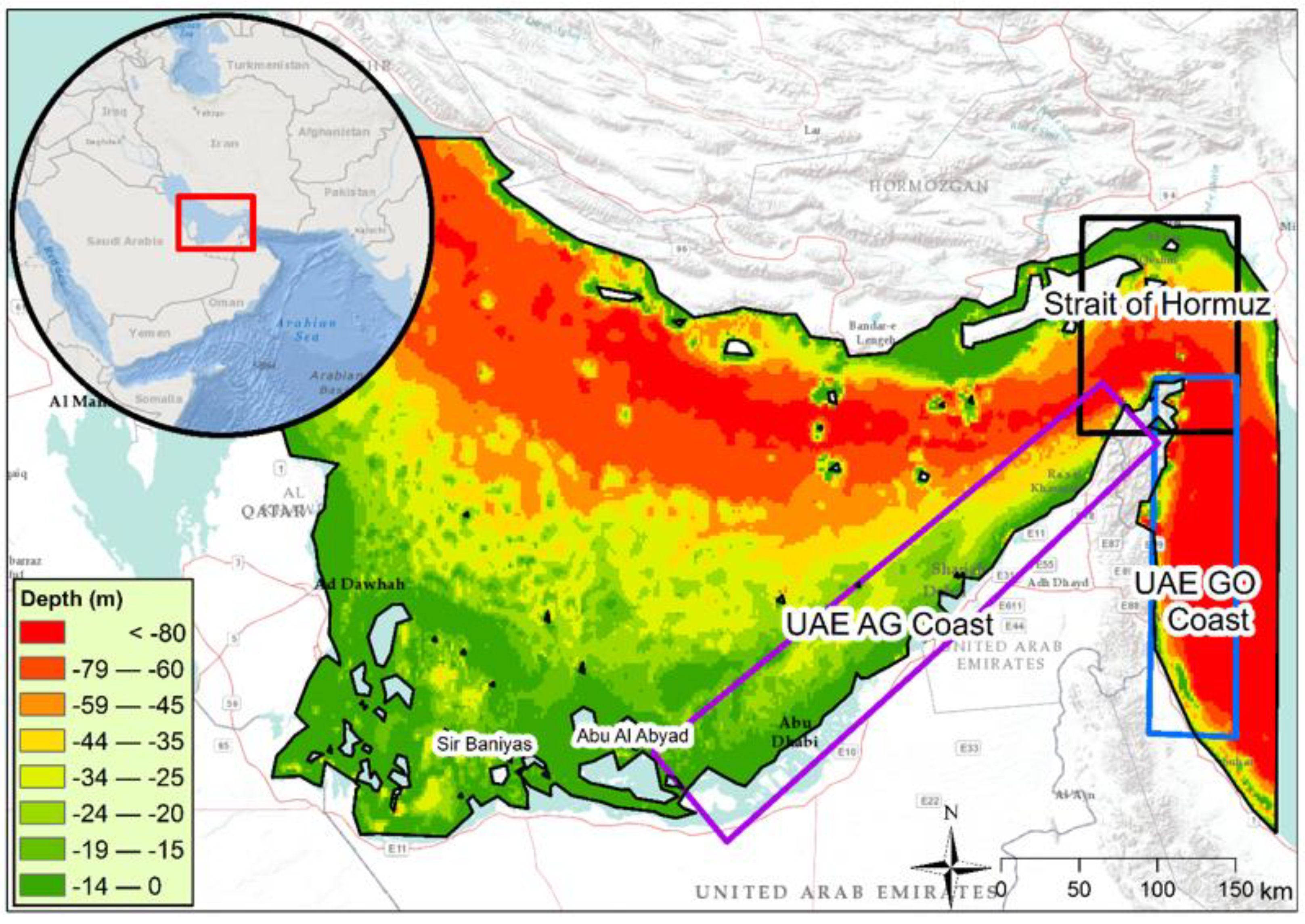
Figure 1.
Map of the study area with bathymetric data of the Arabian and Oman Gulfs and the location of the three sections (UAE Arabian Gulf (AG) Coast, UAE Gulf of Oman (GO), and Strait of Hormuz) that were used for the empirical orthogonal function (EOF) analysis.
2.2. Dataset
2.2.1. Chl-a Data
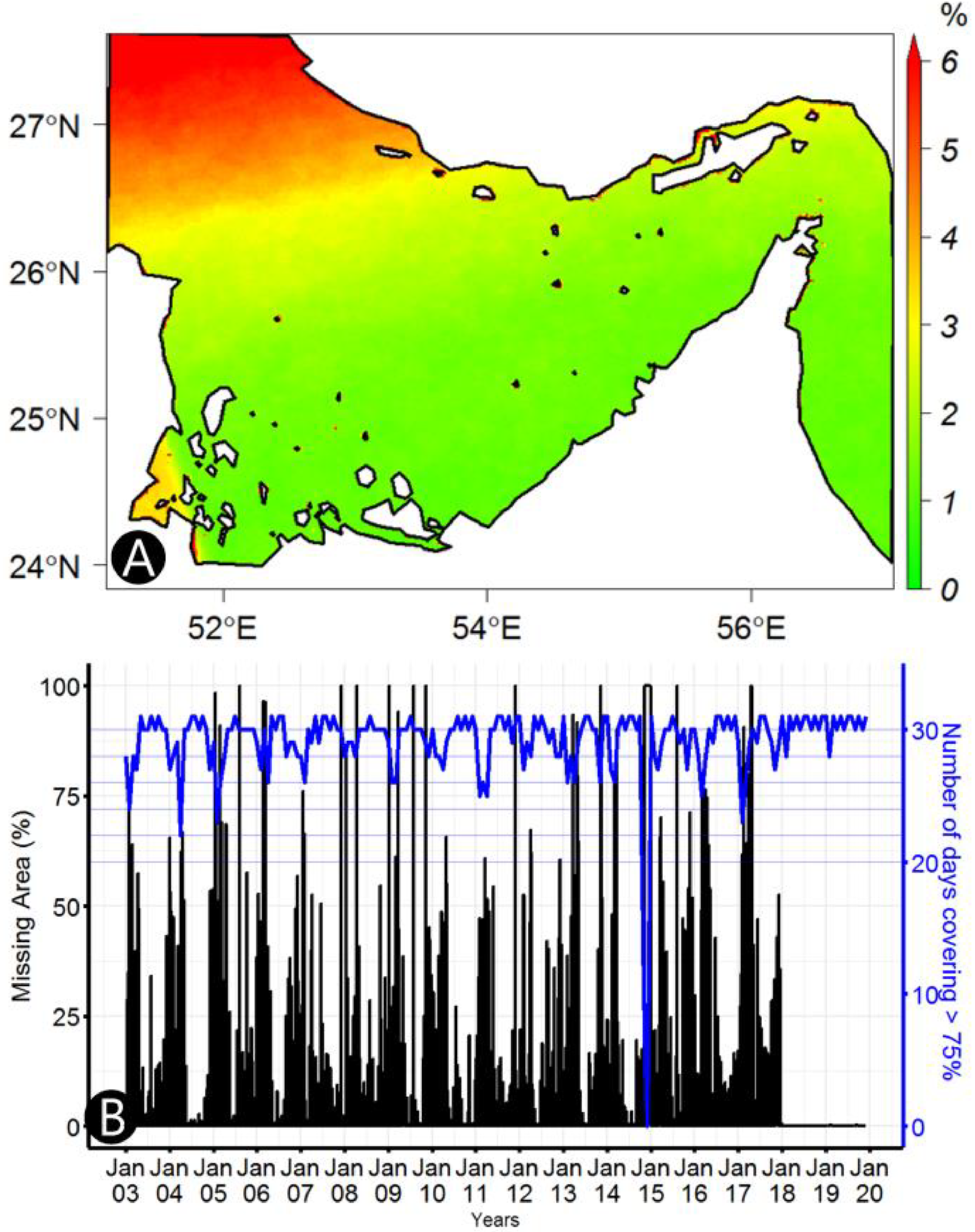
To characterize the spatial and temporal distribution of algal blooms along the coast of the UAE, daily remotely sensed Chl-a concentration and SST were obtained for the period between 2003 and 2019. Level 2 product with a spatial resolution of 1 × 1 km2 of the Chl-a concentration from MODIS onboard Aqua satellite were downloaded from the NASA MODIS standard products at https://oceancolor.gsfc.nasa.gov/cgi/browse.pl. These data are in the netCDF-4 format (.nc), which contains multi-object files [38]. The Band Select of Data Conversion tool from Sentinel Application Platform (SNAP) was used to extract the products of both Chl-a and SST and mosaicked using the Geospatial Data Abstraction Library (GDAL) merge tool by pyQGIS. The Chl-a data contain gaps mainly due to the inability of the sensors to perpetrate through clouds. From the study period (1 January 2003 to 31 December 2019), out of 6208 days, 6149 daily imageries were available in the archive. Out of the available daily images, 217 images were found to be covered by clouds for more than 75% of the study area. The temporal distribution showed that the daily images were missing around 5% of the study area every day before January 2018 (Figure 2B). The spatial distribution suggested that the area that failed to be covered consistently was the northwestern tip (Figure 2A). The areal coverage drops to below 75% during only a few days for a small number of months. Due to a lack of sufficient data, the areas with a dataset that are missing more than 75% (~5% of the study area) of their observations were masked out before the analysis was conducted. The areal average amount of missing data over the entire Arabian Sea was recorded as 16.3%. The month of July had most of the missing data, including on seven occasions wherein the daily images failed to cover more than 25% of the study area. Moradi [39] also suggested that the data of July included the highest missing values in the region followed by August and June.
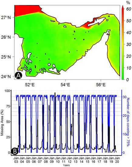
Figure 2.
(A) Spatial distribution of the missing data of the Chl-a concentration across the study area. (B) Temporal distribution of the missing data of the Chl-a concentration (black line represents a daily fraction of missing area and the blue line represents the number of days in a month with data coverage fraction greater than 75%).
2.2.2. SST Data
Level 2 product with a spatial resolution of 1 × 1 km2 of the SST from MODIS onboard Aqua satellite was downloaded from the NASA MODIS standard products at https://oceancolor.gsfc.nasa.gov/cgi/browse.pl. For the MODIS data, thermal channels 31 (10.780 to 11.280 μm) and 32 (11.770 to 12.270 μm) are particularly suited to estimate the surface temperature [40]. The MODIS sea surface temperature data have been widely validated for open waters and therefore are widely accepted as accurate [37,41,42,43,44,45].
The SST data have relatively better coverage than the Chl-a data described above. The study spanned for a period (1 January 2003 to 31 December 2019) of 6208 days, out of which 6144 daily images were available in the archive. The notable missing data from the archive is that only 10 days of data were available for the months of November and December 2014. However, only 19 daily images out of the available 6144 imageries had a missing area of more than 75% of the study area (mainly due to clouds). The temporal distribution of the missing data shows that the cloud coverage is much higher in the winter months (from November to April), as shown in Figure 3B. The areal coverage drops to below 75% during only a few days for a small number of months. The spatial distribution of the missing data indicates that the northwestern tip of the study area is the area with the most missing data (~6%). The areal average of missing data was 2.4%. The amount of missing data decreases as you move from the northwestern to the southeastern corner (Figure 3A). Interestingly, from January 2018 to December 2019, there was no significant missing data (images covered more than 98% of the study area). That is likely due to an enhancement of the product processing algorithm.

Figure 3.
(A) Spatial distribution of the missing data of SST across the study area. (B) Temporal distribution of the missing data of SST (black line represents a daily fraction of missing area and the blue line represents the number of days in a month with data coverage fraction greater than 75%).
2.2.3. Bathymetry Data
The bathymetric data, the Global Relief Model referred to as ETOPO1, which is an improved model of the ETOPO2v2 Global Relief Model, were used in the study. The data are developed by the National Geophysical Data Center (NGDC) of the National Oceanic and Atmospheric Administration (NOAA). The ETOPO1 has two versions—Ice Surface and Bedrock. The Ice Surface version includes the top of the ice sheets (Antarctica and Greenland), while the Bedrock version depicts the base of the ice sheets [46]. For this study, the Bedrock version was used. The vertical datum is referenced from the mean sea level and the World Geodetic System of 1984 (WGS 84) datum was used as a horizontal datum. The spatial resolution of the data is one arcminute with global coverage. The bathymetry of the study area shows a shallow AG and a much deeper GO (Figure 1).
3. Methodology
3.1. Filling Missing Data
Cloud cover significantly obscures surface information; therefore, it is very important to retrieve the Chl-a and SST under overcast skies. The biggest challenge in retrieving the Chl-a and SST is to eliminate cloud contamination. Figure 4 presents how the missing data values and gaps of Chl-a and SST are filled. To fill the missing values of Chl-a, the daily Chl-a data for the study period (2003 to 2019) are used to develop the monthly composites of each Julian day. Then, the missing data values and gaps of the daily data are filled with the corresponding monthly composite values. MODIS cloud-free data composite image (SST, monthly composite product) was employed to fill in these missing pixels’ values of SST. This method was used because the amount of missing data is not as significant relative to the other regions of the world where cloud cover is a major issue. For example, Li [47] found that only 2872 daily snapshots were useful out of 3653 imageries in the Gulf of Maine. However, in this study, only 217 days of Chl-a had missing data covering more than 75% of the study area out of 6149 obtained daily images. The northwestern part of the study area was found to have significant gaps in the data. For this reason, the area which covers ~5% of the total study area was masked from the analysis. The average missing data across the study period for Chl-a was around 10%. Conversely, the average missing data of SST is ~2% of the study area after excluding the northwestern part of the study area.
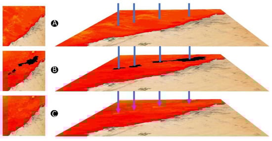
Figure 4.
Presents how the data values of Chl-a and SST are filled. (A) Monthly composites of the Julian day. (B) Original daily data with missing values and gaps (black spots are missing values). (C) Filled data.
3.2. Empirical Orthogonal Function (EOF) Analysis
The primary application of EOF is that it helps in understanding the spatial patterns of variability in spatiotemporal data by examining the EOF coefficient maps. Secondly, it can be used to reduce the dimension of the components by using the optimal number of components that explain the majority of the variability in the spatiotemporal dataset [48,49]. The EOFs analysis was conducted over the coastal areas of the UAE, the AG Coast, Strait of Hormuz, and GO Coast (Figure 1) to examine the spatial variability of the SST and Chl-a concentration.
The raw data matrix F is arranged in a matrix format M × N, where M is the time series dimension and N is the space dimension. The covariance matrix R is calculated using Equation (1). Then, the eigenvalues are solved with Equation (2), which provides the information about the amount of variability explained by each component [48]. The highest three components were selected for this study as they explain more than three-quarters of the variability in both Chl-a and SST.
is a diagonal matrix containing eigenvalues of R where i is the length of the time series ranges from 1 to (size of ). The column vectors of are the eigenvectors of that corresponds to the eigenvalues which contain information about the spatial distribution of the eigenvalues.
The raw data can be reconstructed from the EOFs and the eigenvectors using the following:
The amount of variability explained by one EOFs component a can be estimated as a fraction of the total variability using Equation (4).
3.3. Correlation Analysis
The Pearson correlation coefficient (PCC) statistical tool was used to evaluate the impact of SST on Chl-a concentration. If the value approaches 1/−1, it indicates that the relationship is strongly positive/negative, and if the coefficient is closer to 0, it indicates that the relationship between the variables is weak. Cross-correlation was conducted to assess the possible lag time of the impact of the SST over the formation of the Chl-a concentration. The mathematical formula used is obtained from Pearson [50]:
where n is the sample size, and are records of the variables (SST and Chl-a in this case), and are the average values of the variables, and and are the standard deviations of the variables.
3.4. Correlated Seasonal Mann–Kendal Trend Test
The corrected seasonal Mann–Kendal trend test was used to investigate the presence of a significant trend in the data. This test was a modified version of the original Mann–Kendal test to accommodate seasonally correlated data. The adjustment was used by Hirsch [51] and Libiseller [52] to reduce the seasonal autocorrelation in the dataset. The Mann–Kendall scores are first computed for each month separately as follows:
where is a sign function obtaining the sign of real number, xij and xik are monthly series values for the periods and , respectively, and i represent the month. The variance for each month is given by:
where is the number of tied groups for the ith month and is the number of observations in the pth group for the ith month. Then, the Mann–Kendall score and variance for the entire series are computed as follows:
where is the Mann–Kendall score of an individual month and m, the number of months in this study, is 12. Similarly, is the variance of individual months. The seasonal adjusted Mann–Kendall test statistics for the series () is given by:
Finally, for the areas with a significant trend, the magnitude of the trend was computed using a linear model (y = α + βx). Moreover, trend analysis was conducted over the summer and winter months separately to assess the influence of seasonality.
4. Results and Discussion
4.1. Spatiotemporal Distribution of Chl-a and SST
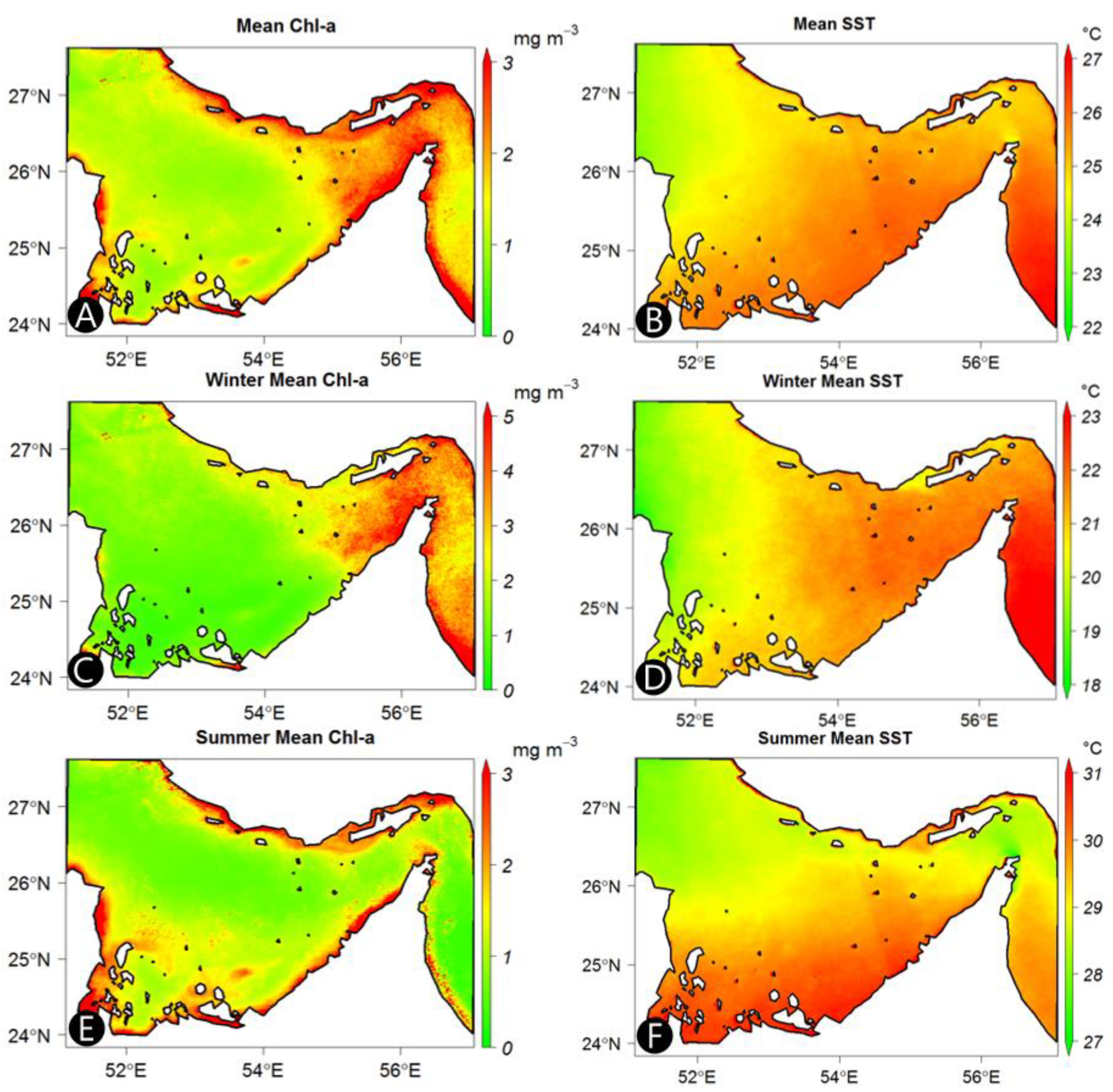
The spatial distribution of the long-term average of Chl-a concentration was unevenly distributed across the Arabian Sea. The Chl-a concentration was high in the coastal areas and the Strait of Hormuz (Figure 5A). The coastal hotspots of Chl-a concentration are usually created due to the loading of nutrients with the discharge from the Wadis and artificial loading of nutrients from agricultural and aquaculture activities around the shores [3,5]. The areal average concentration of Chl-a in the Strait of Hurmuz was 2.8 mg m−3, whereas the areal average concentration across the entire study area was 1.7 mg m−3. The seasonal distribution shows that February and March are the months with the highest Chl-a concentration, especially in the Strait of Hormuz and GO (Appendix A). The main reasons for such a high concentration of Chl-a in the Strait of Hormuz are seasonal upwelling, mixing of the AG and GO, and the high concentration of pollutants and river discharge from the northern coast [53]. Over the study period of 17 years, 2008 and 2009 showed peak concentration of Chl-a with an average concentration of 2.4 mg m−3 and 2.1 mg m−3, respectively (Appendix C). This period includes the red tide events that were reported by Richlen [54]. Moreover, the seasonal mean distribution showed a distinct pattern between winter and summer. The winter had a higher concentration of Chl-a, which was clearly observed in the Strait of Hormuz (Figure 5C). However, in summer, the coastal areas exhibited a relatively high concentration of Chl-a (Figure 5E).
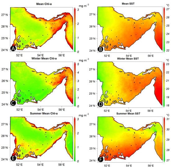
Figure 5.
Spatial distribution of the long-term average of (A) Chl-a concentration, (B) SST, (C) long-term winter Chl-a average, (D) long-term winter SST average, (E) long-term summer Chl-a, and (F) long-term summer SST average across the Arabian Sea (Arabian and Oman Gulfs) during the study period (1 January 2003 to 31 December 2019).
The spatial distribution of the long-term average of Chl-a concentration was unevenly distributed across the Arabian Sea. The Chl-a concentration was high in the coastal areas and the Strait of Hormuz (Figure 5A). The coastal hotspots of Chl-a concentration are usually created due to the loading of nutrients with the discharge from the Wadis and artificial loading of nutrients from agricultural and aquaculture activities around the shores [3,5]. The areal average concentration of Chl-a in the Strait of Hurmuz was 2.8 mg m−3, whereas the areal average concentration across the entire study area was 1.7 mg m−3. The seasonal distribution shows that February and March are the months with the highest Chl-a concentration, especially in the Strait of Hormuz and GO (Appendix A). The main reasons for such a high concentration of Chl-a in the Strait of Hormuz are seasonal upwelling, mixing of the AG and GO, and the high concentration of pollutants and river discharge from the northern coast [53]. Over the study period of 17 years, 2008 and 2009 showed peak concentration of Chl-a with an average concentration of 2.4 mg m−3 and 2.1 mg m−3, respectively (Appendix C). This period includes the red tide events that were reported by Richlen [54]. Moreover, the seasonal mean distribution showed a distinct pattern between winter and summer. The winter had a higher concentration of Chl-a, which was clearly observed in the Strait of Hormuz (Figure 5C). However, in summer, the coastal areas exhibited a relatively high concentration of Chl-a (Figure 5E).
Unlike Chl-a concentration, the spatial distribution of the average SST for the period 2003 to 2019 shows a uniform linear increase in the west–east direction, as shown in Figure 5B. The GO experienced an average SST of about 26 °C, which makes it the hottest region in the study area. The areal average SST over the entire study area was around 25 °C. A difference of ~3 °C was observed between the hottest region (GO) and the coldest region (northwestern AG) in the long-term average of SST. The monthly distribution of SST showed very little spatial variability (Appendix B). The annual average suggests that the hottest years were 2018 and 2019 with an average SST of 26. 3 °C and 26. 4 °C, respectively (Appendix D). The AG and GO experience different winter and summer temperature patterns. The southern AG was warmer than GO in the summer (Figure 5F), whereas the GO was warmer than AG in the winter (Figure 5D).
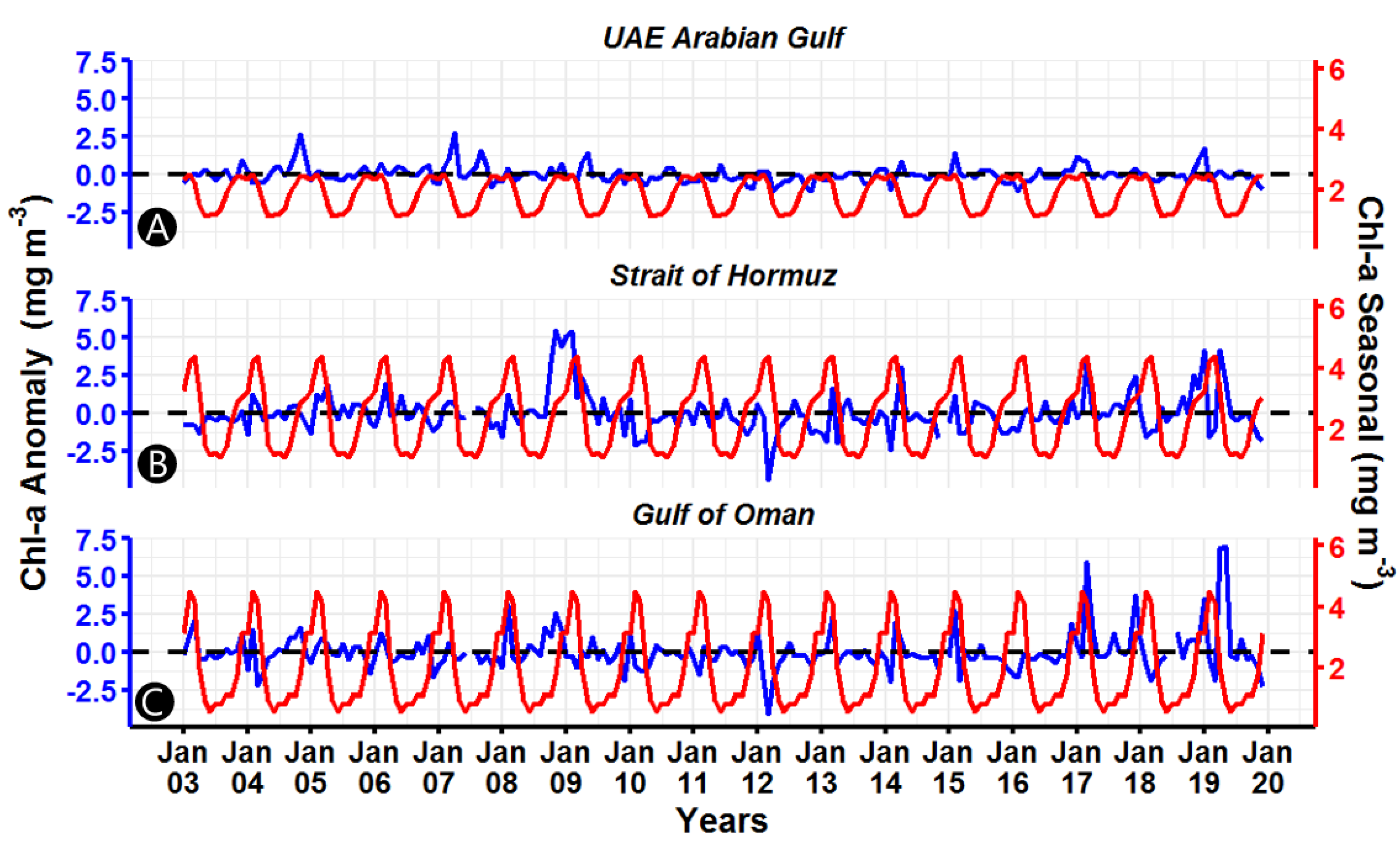
The temporal distribution of the Chl-a concentration suggests that different parts of the Arabian Sea express different seasonal variability. The shape of the seasonal cycle appears to be a smooth sinusoidal curve with relatively smaller amplitude in the case of the AG coast of UAE and a more pointed shape with a higher variability for both the Strait of Hormuz and the GO. The UAE’s coast across the AG experiences small seasonal variability with the peak concentration seen in November and the lowest concentration observed in May (Figure 6A). The highest variability is seen in the time series of the GO with the peak concentration observed in February and the lowest reported in May (Figure 6C). In the summer of 2012 (April, May, and June), the entire region experienced the lowest concentration of Chl-a (Figure 6). After that point, the Chl-a concentration was above normal in winter and below normal in the summer, especially in the Strait of Hormuz and the GO.
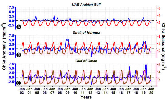
Figure 6.
The time series of Chl-a concentration across different sections of the Arabian Sea (A) UAE Arabian Gulf coast, (B) Strait of Hurmuz, and (C) Gulf of Oman coast (the red line is the seasonal cycle, which is the average of each month; the blue line is the anomaly, which is the difference between monthly average and seasonal cycle).
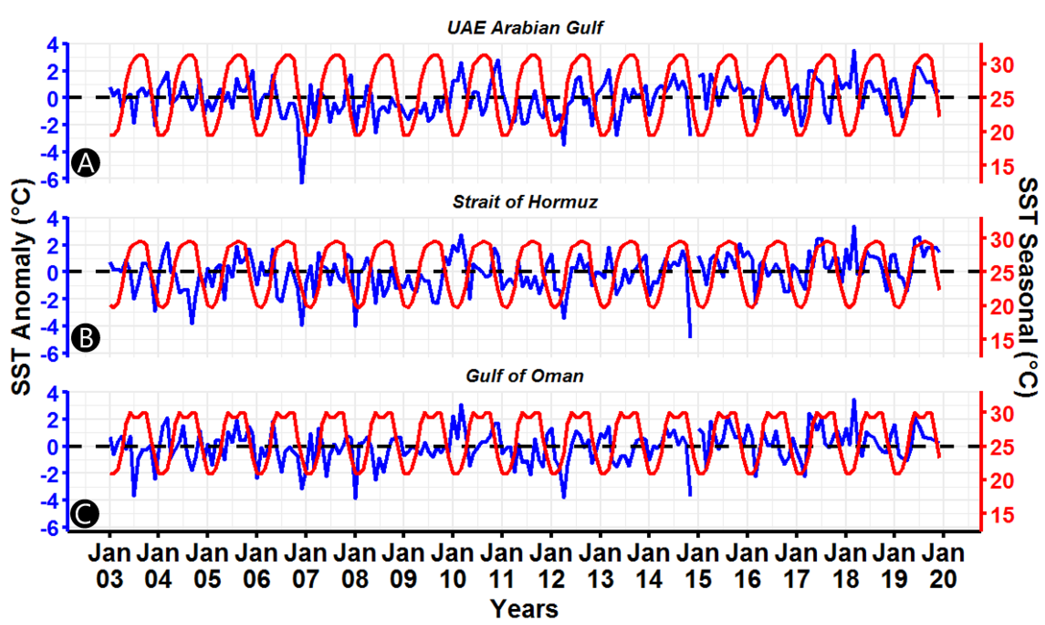
The temporal distribution of SST reveals different behaviors among the three sample regions. The UAE’s AG coast showed a smooth sinusoidal seasonal cycle with the highest variability between winter and summer (Figure 7). The SST ranges from 19 °C in January to as high as 31 °C in September. The GO showed a bimodal seasonal cycle with peaks in June (30 °C) and September (30 °C) and February as the coldest month with 21 °C (Figure 7). This bimodal cycle is due to the decrease of the temperature during the southwest monsoon that occurs from June to September [55]. The time series showed that the Arabian Sea, in general, experienced cooler than usual winters between 2005 and 2008. Towards the end of the study period (2014 to 2019), the summers became hotter than the typical summer. The northeast monsoon is the main reason for cool SST across the entire AG and the GO from November to March [56].
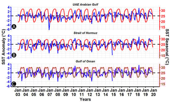
Figure 7.
The time series of SST across different sections of the Arabian Sea (A) UAE Arabian Gulf coast, (B) Strait of Hurmuz, and (C) Gulf of Oman coast (the red line is the seasonal cycle, which is the average of each month; the blue line is the anomaly, which is the difference between monthly average and seasonal cycle).
4.2. Variability in Chl-a and SST
The best way to display the EOFs components as meaningful indicators is to represent them as homogeneous correlation maps. The homogenous correlation map of the EOFs’ first component is the correlation of the raw data with the expansion coefficient of the first component of EOFs [57]. With regard to the mode of variability of the Chl-a concentration, the first three components captured 74% of the variability on average. The first component, which explains 42% of the variability, had a strong relationship in the Strait of Hormuz and GO, as shown in Figure 8A. The first component is related to the northeast monsoon winds that move heat from the surface of the Arabian Sea, which occurs from early November to March. Lower solar radiation and increased salinity create convective mixing that drives upward transport of nutrients [2]. The availability of nutrients with optimal atmospheric conditions results in excessive growth of phytoplankton biomass. The second component, with an average variability of 24%, had the reverse impact of the first component with the western coast of the UAE affected significantly more than the rest of the area (Figure 8B). The spikes of Chl-a concentration over the coast of UAE (AG) at the end of 2004, 2007, and 2018 to 2019 were related to the second component (Figure 8D). The third component, responsible for 8% of the variability, was highly related to the Strait of Hormuz, which captured the peaks in Chl-a concentration observed in 2008 to 2009 (Figure 8D). The 2008 to 2009 algal blooms were catastrophic to the infrastructure of the countries in the AG, especially in the water supply system and tourism industry. The blooms dissipated in August 2009 about nine months after they first appeared on the coast [54].
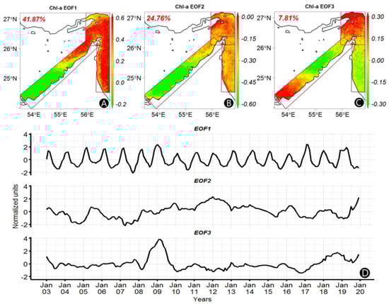
Figure 8.
Spatial distribution of the homogenous correlation map of the first three EOFs components of the Chl-a concentration ((A–C), respectively), and their time-series component (D).
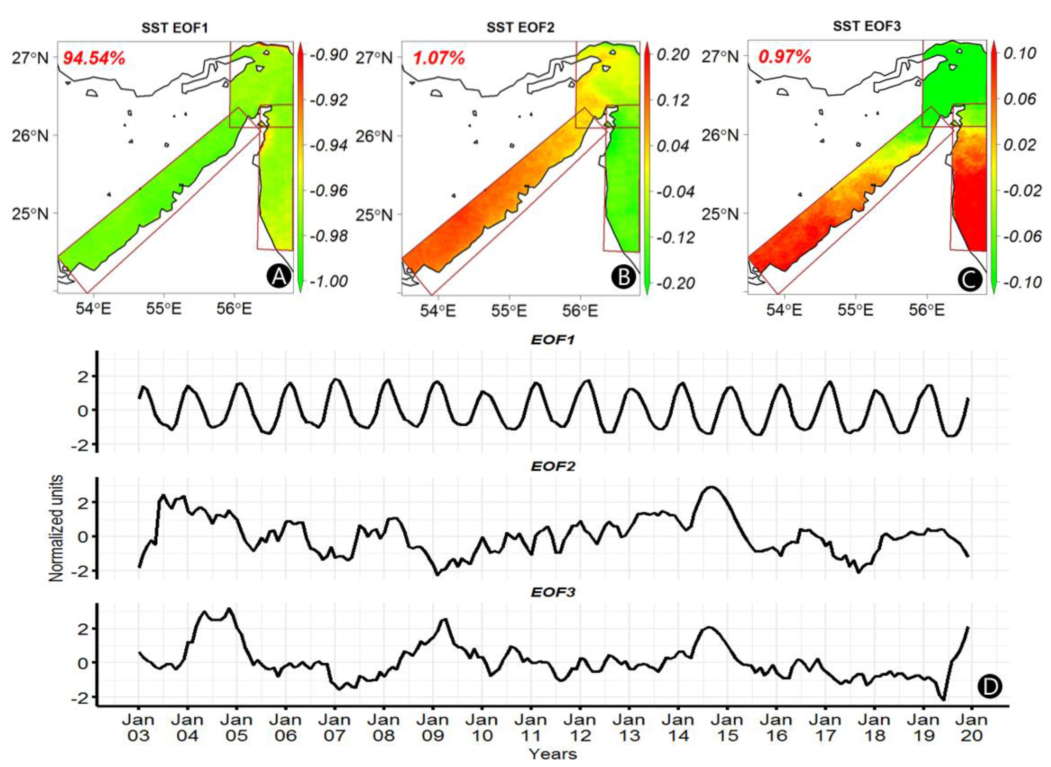
The first three EOFs modes of SST captured more than 96% of the variability in the dataset. The first EOF component, which represents the annual seasonal component of SST, accounts for more than 94% of the variability, as shown in Figure 9A. The entire study area showed a strong homogeneous correlation coefficient of more than 0.9. This means that the EOF first component is highly influenced by the annual periodicity that reaches its peak in summer and its lowest in winter. The spatial variability is very small, indicating that the seasonal variability is uniform across the entire area. This shows that the annual variability of the SST (that represents 95% of the total variability) showed a very small spatial variability across the coasts of the UAE. This is evident in the fact that the entire UAE coast demonstrates an interquartile range of only 0.7 °C in the long-term average SST. However, the second EOF component of SST, accounting for 1.07% of the total variance, showed a significant spatial variability (Figure 9B). The UAE’s AG coast is positively correlated, whereas the GO coast is negatively correlated. The second component seems to capture the impact of the southwest monsoon with a spatial variability that is oriented in the east–west direction. The southwest monsoon decreases the temperature of the GO, causing a bimodal cycle. The southwest monsoon does not have a significant impact on the SST of the AG; on the contrary, SST increases during that period. This result is in line with the findings of Nandkeolyar [56]. The third component of SST also revealed a significant spatial variability, whereas the Strait of Hormuz is negatively correlated and the rest of the coasts are positively correlated. The spatial variability is oriented in the north–south direction (Figure 9C).

Figure 9.
Spatial distribution of the homogenous correlation map of the first three EOFs components of the SST ((A–C), respectively), and their time-series component (D).
4.3. Correlation of Chl-a and SST
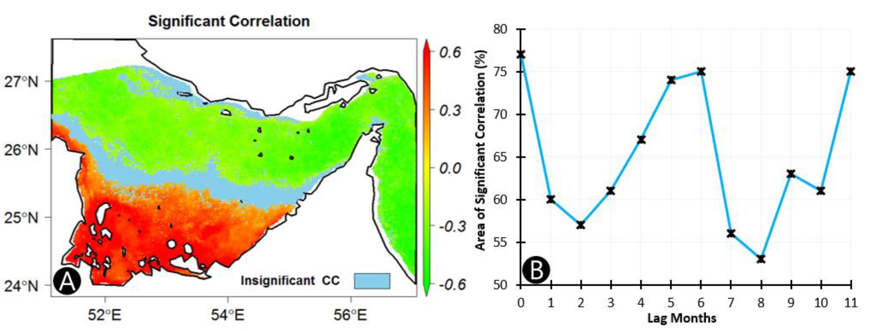
The correlation coefficient of Chl-a and SST indicates that around 75% of the study area exhibits significant correlation as shown in Figure 10A. The coastal area of western UAE showed a significant positive correlation which suggests that the SST affects the concentration of Chl-a. However, more than half of the study area indicated that SST negatively influenced the Chl-a concentration in the AG and GO, whereas more than a quarter of the area showed a positive relationship. The southern coast of the AG showed a significant positive correlation coefficient of 0.44 on average and standard deviation (SD) of 0.15. The areas with positive correlation had an average Chl-a of 1.36 mg m−3 (SD of 0.51 mg m−3) and an average SST of 25.39 °C (SD of 0.61 °C). On the other hand, the negatively correlated areas had an average correlation coefficient of −0.33 (SD of 0.09). The negatively correlated areas have shown a compact distribution of the correlation coefficient despite covering an area almost twice the size of the positively correlated areas. This shows that the variability in the negatively correlated areas is small relative to the positively correlated places. The average Chl-a of the negatively correlated areas was 1.66 mg m−3 (SD of 0.66 mg m−3) and the average SST was 25.18 °C (SD of 0.77 °C). Additionally, cross-correlation analysis revealed that the best correlation between Chl-a and SST was found without any lag, i.e. the largest area with a significant correlation coefficient (Figure 10B).

Figure 10.
(A) The spatial distribution of the correlation coefficients over the Arabian and Oman Gulfs. (B) The relationship between the percentages of the area with a significant correlation coefficient and the time lag of the SST (zero meaning without any lag).
The spatial distribution of the correlation indicates that the UAE’s AG coast showed a positive correlation between the Chl-a concentration and the SST and especially coasts near the Abu Al Abyad and Sir Baniyas islands. However, the northeastern coast of the UAE (from Dubai northward) showed a significant negative correlation covering around one-third of the study area. Along the coasts of the GO and the Strait of Hormuz, the correlation was almost uniform, with more than 80% of the area showing a negative correlation. Detailed summary statistics of the correlation in the three regions are shown in Table 1.

Table 1.
Basic statistics of the variables in the three main regions of interest.
Moreover, the relationship between the Chl-a concentration and the SST was highly dependent on the bathymetry of the seawaters. This relationship is due to the difference in gaining the solar heat between the shallow (warmer) and deeper portions (colder) of the sea. The deeper sea areas have greater thermal memory; in turn, they require a longer time to heat and never reach the optimum temperature for algal blooms (Chl-a) growth. Therefore, the surface water in the middle (deep) sea generally gains lower temperature than the surface water near the shore [16]. All the areas that showed a significant positive correlation were in the shallow coastal areas. On the contrary, the deeper areas seem to have an inverse relationship between Chl-a and SST (Figure 11). In the areas where the depth of the sea is less than 20 m below sea level, the average correlation coefficient between Chl-a concentration and SST was 0.43, whereas an average correlation of −0.34 was found in waters deeper than 40 m. Moreover, the areas that did not exhibit a significant correlation have an average depth of 33 m and a median of 28 m below the sea level. This means an increase in SST increases the concentration of Chl-a in shallow water with less than 20 m depth, while an increase in SST tends to decrease the concentration of Chl-a in the deeper waters below 40 m sea level. The full relationship between the bathymetry and the correlation of the Chl-a and SST concentration is shown in Figure 11B.
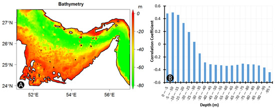
Figure 11.
(A) Bathymetry of the Arabian Gulf and Gulf of Oman. (B) The relationship between the correlation coefficient and the depth of the seawater.
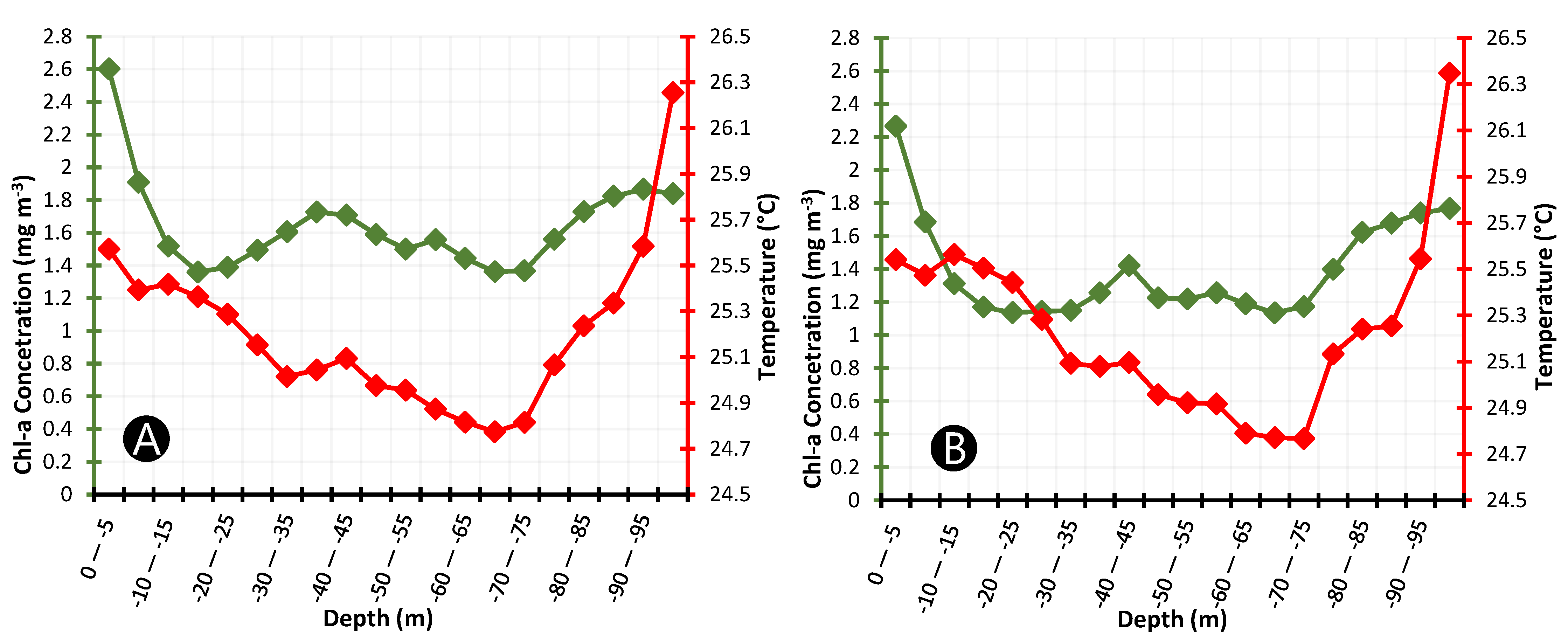
The relationship between bathymetry, Chl-a, and SST follows a U-shaped curve with the shallow and very deep seas having higher Chl-a and SST, respectively, as shown in Figure 12. The shallow waters experienced the highest Chl-a concentration in terms of average and median values. The deeper areas were observed to have the highest SST (Figure 12). Eventually, as the depth increases, both Chl-a and SST start to decline rapidly until 20 m below sea level. Then, the Chl-a concentration remains relatively stable while SST decreases until it reaches 24.7 °C at a depth of 70 m. Then, the SST begins to increase, reaching more than 26 °C at the depth of >95 m while the Chl-a also rises but at a lower rate, reaching 1.8 mg m−3 from 1.4 mg m−3. The deepest region is the GO with the highest SST was also one of the areas with a high concentration of Chl-a.
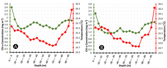
Figure 12.
The relationship between the Chl-a and SST with respect to the depth of the seawaters using (A) the long-term average and (B) the long-term median of Chl-a and SST.
4.4. Trend Analysis
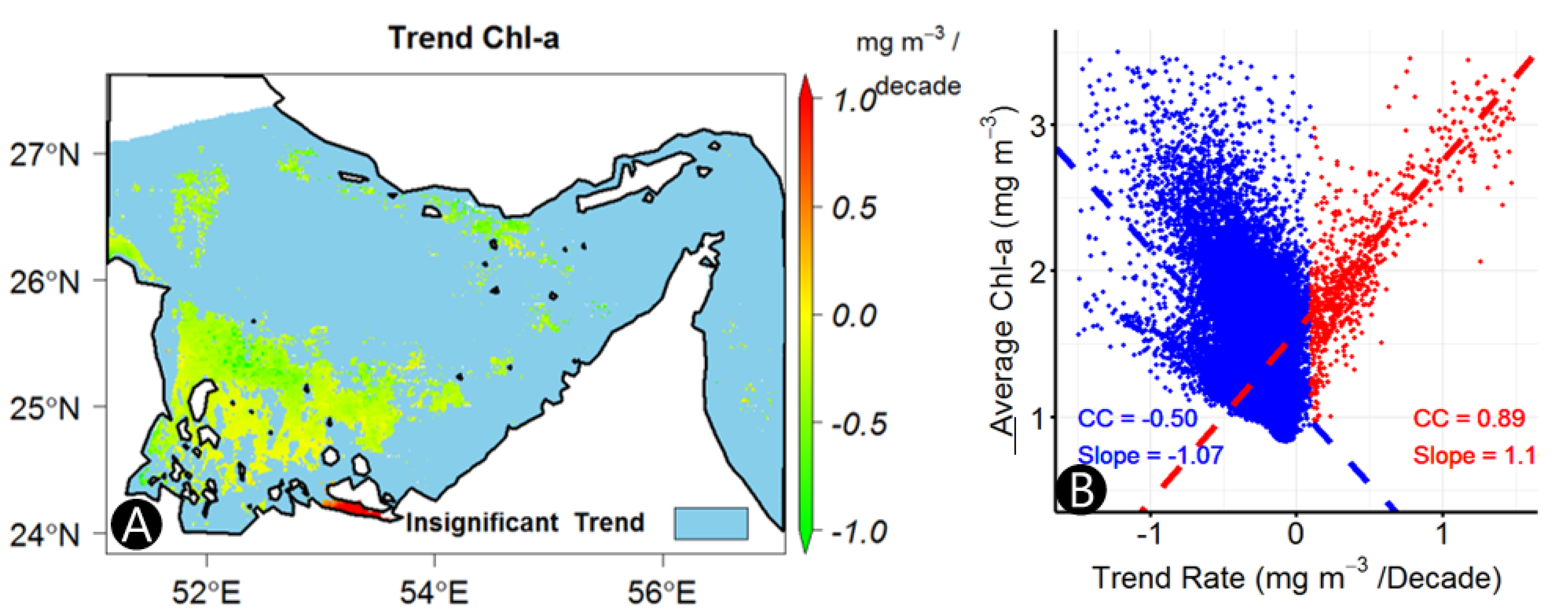
Mann–Kendal trend analysis was carried out to investigate the possibility of a significant trend in both variables (Chl-a and SST) over the span of 17 years. The Chl-a showed a decreasing trend in most areas, except on the coast of Abu Al Abyad Island, which is located in the western part of the UAE. This is mainly due to nutrient leaching from the orchards’ soil and aquafarming drainage that contains nutrients useful for algae growth. Overall, 21% of the study area had a significant trend in Chl-a concentration. The majority (95%) of this area experienced a decreasing trend in the concentration of the Chl-a with an average of −0.28 mg m−3 per decade rate of decline (Figure 13A). The decreasing trend appears to increase in areas with higher average Chl-a concentration (Figure 13B). This suggests that the concentration of Chl-a is decreasing and at a higher rate in areas with a relatively high concentration during the last two decades. However, the areas with the highest concentration of Chl-a (Strait of Hormuz and the GO) did not experience a significant trend. In the places where the trend was increasing (Abu Abyad Island), the trend rate was increased as the average concentration increased. This is mainly due to the agricultural and aquaculture activities involved in Abu Abyad Island and the results suggest that the activities have increased over time (Figure 13B).
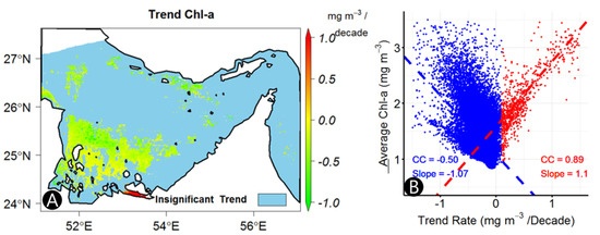
Figure 13.
(A) Spatial distribution of the estimated trend using linear regression over the Arabian and Oman Gulfs for Chl-a and (B) scatter plot of the estimated rate of trend versus the long-term average of Chl-a concentration. Red points represent a positive trend and blue points represent a negative trend (n = 35,358).
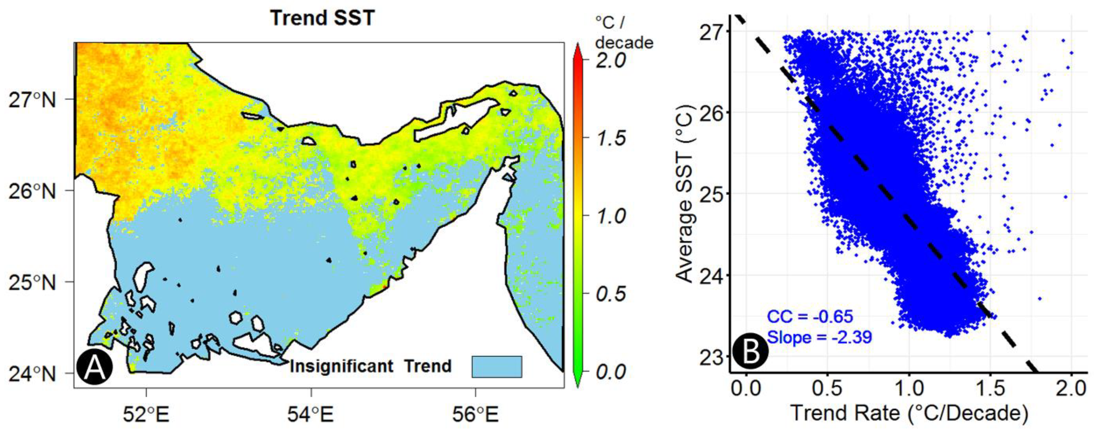
The trend test indicated that 52% of the study area, mainly located in the northern part, experienced a significant SST-positive trend (Figure 14). The average rate of increase in these regions is estimated as 0.91 °C per decade. Most of the areas that showed an increasing trend are places with relatively lower mean SST. As the long-term average SST decreases, the rate of trend increases sharply, as shown in Figure 14B. This means that the cooler regions of the AG are experiencing an increase in temperature at an alarming rate.

Figure 14.
(A) Spatial distribution of the estimated trend using a linear regression model over the Arabian and Oman Gulfs for SST and (B) scatter plot of the estimated rate of trend versus the long-term average of SST (n = 85,693).
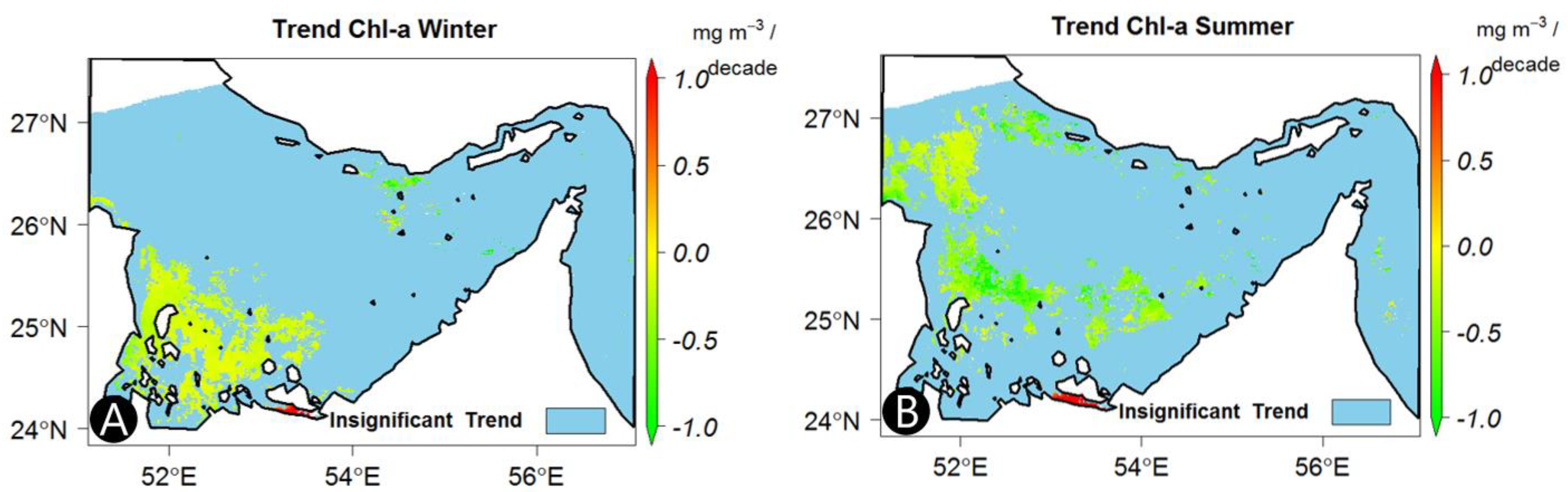
The trend in both the winter and summer seasons has been further analyzed to investigate the seasonality of the trends. The time series is divided into two six-month periods of summer and winter. Summer months (May to October) are categorized as very hot and humid and the winter months (November to April) are characterized by relatively cooler months (Appendix B). The seasonal trend analysis of the Chl-a indicated that 18% and 13% of the study area have a significant trend for the months of summer and winter, respectively. Less than 1% of the area with a significant trend showed a positive trend. The Abu Abyad Island and its surroundings showed an increasing trend in both seasons. This further supports the aforementioned reasoning that the higher concentration of Chl-a near the island is not related to climatological phenomena but to activities on the island. The spatial distribution showed that the trend in the winter is concentrated in the coastal area located between Qatar and UAE, whereas in summer, the trend is experienced further from the seashore (Figure 15A,B). The rate of decline was higher during summer with an average rate of −0.41 mg m−3 compared to the average rate of −0.22 mg m−3 in winter. Similar to the results of the trend analysis, the areas with higher average Chl-a concentration (Strait of Hormuz and GO as shown in Figure 2B) did not show a significant trend in both seasons over the last two decades.

Figure 15.
Spatial distribution of the seasonal trend of Chl-a in (A) winter (November to April) and (B)summer (May to October).
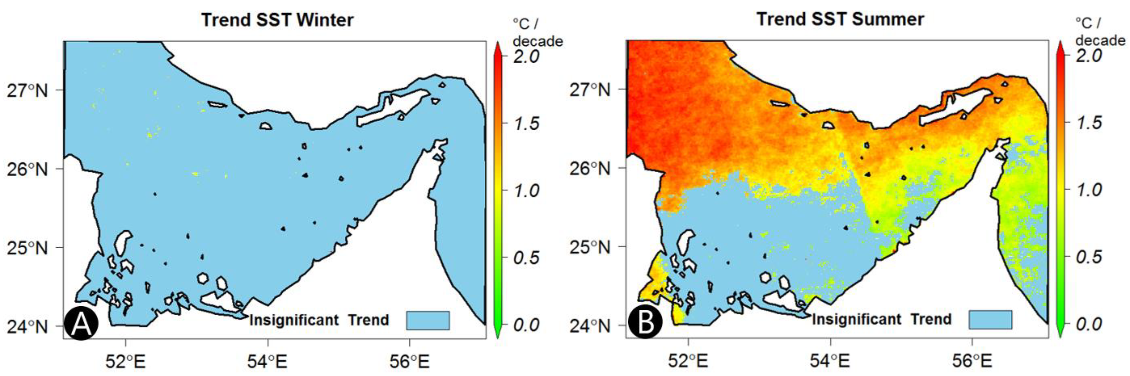
The seasonal trend analysis of the SST showed that the winter months had no significant trend over the entire area (Figure 16A). On the contrary, the summer was the dominant season of the trend. The summer months demonstrated an increasing trend in more than two-thirds of the study area (Figure 16B). The results indicated that the summer months are becoming hotter at a rate of higher than 1.0 °C per decade in half of the area. Around 20% of the study area (almost all of them located in the northeastern tip) exhibits an increasing trend rate higher than 1.5 °C per decade. The regions that are warming at a higher rate are the areas with relatively lower average SST. Previous studies also reached a similar conclusion, which indicates that the summer months are becoming hotter at a much higher rate [56,58]. Piontkovski [58] showed that the trend of SST in June and July was more than double the trend of average annual SST.

Figure 16.
Spatial distribution of the seasonal trend of SST in (A) winter (November to April) and (B) summer (May to October).
5. Summary and Conclusions
The ecosystems of the Arabian seas (Arabian Gulf, Gulf of Oman, and Arabian Sea) are fragile and susceptible to pollution. Among these pollutants are algal blooms. The most effective approach for estimating the Chl-a concentration and assessing the spatiotemporal distribution of algal blooms is the employment of remotely sensed data and remote sensing techniques. This study analyzed the spatiotemporal variability of the Chl-a concentration and SST in the Arabian Gulf and the Gulf of Oman along the UAE coasts. The correlation between the Chl-a and SST is also investigated as it sheds light on the impact of the SST on the growth of phytoplankton. The variability of both Chl-a and SST is also examined using the empirical orthogonal function (EOF) analysis, which helps in understanding the impact of major wind currents in the area.
The spatial distribution of the Chl-a concentration showed that the highest concentration was observed in the Strait of Hormuz with an average of 2.8 mg m−3, which is 1.1 mg m−3 higher than the average for the entire study area. The Gulf of Oman was also the hottest region with an average of 26 °C, which is one degree hotter than the average of the total area. Moreover, SST showed a uniform gradient in the northwest to southeast direction. The summer months (May to October) were the hottest months, with an average of ~31 °C, whereas in the winter months (November to April), the SST reached as low as ~19 °C.
The first EOF component of Chl-a is related to the northeast monsoon winds (November to March), which cools the sea surface. The Chl-a concentration increased in the Strait of Hormuz and the Gulf of Oman due to the availability of nutrients in addition to the optimal atmospheric conditions. The spikes in concentration over the coast of UAE (AG) at the end of 2004, 2007, and 2018 to 2019 were related to the second component.
Three quarters of the study area experienced a significant correlation between the Chl-a and SST. The coastal areas of western UAE and Qatar showed a significant positive correlation, which suggests that the SST affects the concentration of Chl-a. However, more than half of the study area indicated that SST negatively influenced the Chl-a concentration in the Arabian Gulf and the Gulf of Oman, especially areas in the deep sea. Furthermore, the correlation coefficient and the bathymetry of the seas showed a strong relationship. The shallow areas had a strong positive correlation between the SST and Chl-a, whereas the deeper areas were inclined to have a negative correlation.
Lastly, trend analysis was carried out to investigate the presence of significant trends using the correlated seasonal Mann–Kendal trend test. The Chl-a data showed the presence of a trend in just 21% of the study area, of which 95% indicated a decreasing trend. Most of the area with a decreasing trend is located in the southern region, which is closer to the coasts of the UAE and Qatar. The rate at which the trend is decreasing is also related to the average Chl-a concentration. Higher average values of Chl-a concentration are associated with a higher rate of decline, and vice versa. The SST also showed the presence of a significant trend in more than 52% of the study area. However, in this case, an increasing trend is observed. Similarly, the rate of trend showed an inverse relationship with the average SST, the higher the average SST, the smaller the rate of increase, and vice-versa.
The main limitations of the study are the missing data due to cloud cover and the relatively short period of the dataset (2003 to 2019). Even though a mature technique of filling the data was followed, a relatively large amount of missing data can cause uncertainty in the results. The conclusions of this research were similar to previously conducted studies. However, the authors feel that these limitations are worth mentioning.
Author Contributions
K.A.H. and K.A.A. guided this research and contributed significantly to preparing the manuscript for publication; K.A.H., P.P., K.A.A., N.A.H. and H.O.S. developed the research methodology; K.A.H., K.A.A., P.P. and D.T.G. downloaded and processed the remote sensing products; D.T.G. and P.P. developed the scripts used in the analysis. K.A.H., K.A.A., N.A.H., H.O.S. and D.T.G. prepared the first draft; K.A.H., D.T.G., K.A.A. and H.O.S. performed the final overall proofreading of the manuscript. All authors have read and agreed to the published version of the manuscript.
Funding
This research was partially funded through the UAEU Research and sponsored Projects Office (Grant: G00002687).
Data Availability Statement
Publicly available datasets were analyzed in this study. Chlorophyll-a Level 2 data can be found at [https://oceancolor.gsfc.nasa.gov/cgi/browse.pl?sen=amod]. Publicly available datasets were analyzed in this study. SST Level 2 data presented in this study are openly available at [https://podaac.jpl.nasa.gov/dataset/MODIS_A-JPL-L2P-v2019.0] at [doi: 10.5067/GHMDA-2PJ19].
Acknowledgments
The United Arab Emirates University—Research Affairs is gratefully acknowledged for their support. Gratitude is also extended to Marwan Almubarak and Rowan and Linda Hussein for following up with editing.
Conflicts of Interest
The authors declare no conflict of interest.
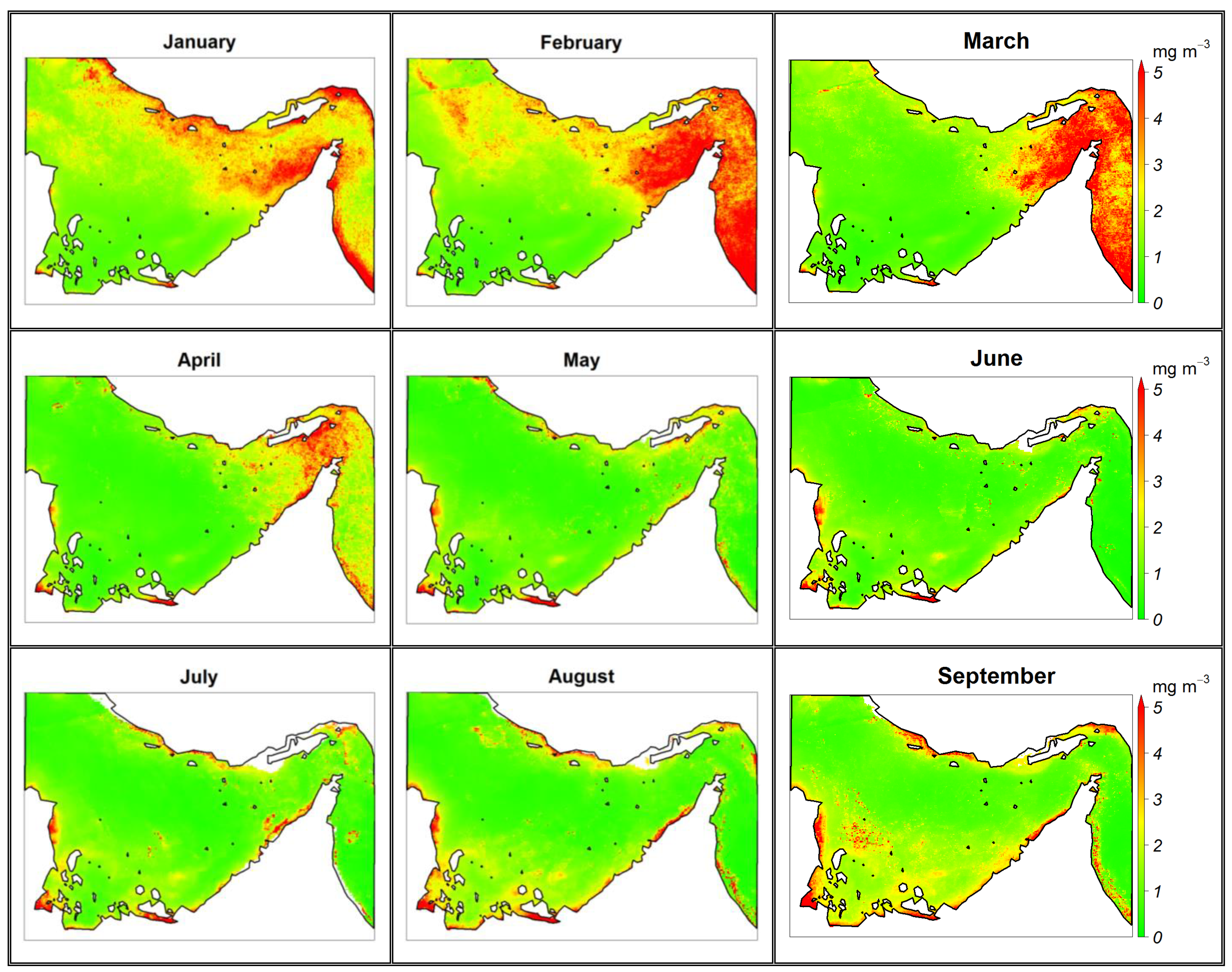
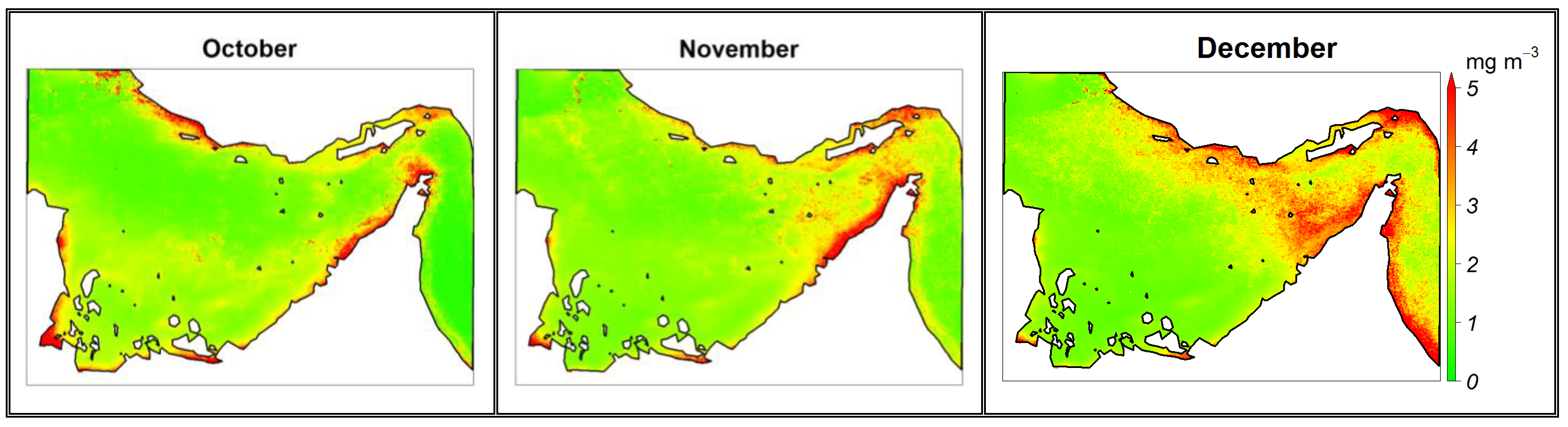
Appendix A

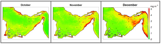
Figure A1.
The spatial distribution of the average monthly Chl-a concentration across the Arabian and Oman Gulfs.
Figure A1.
The spatial distribution of the average monthly Chl-a concentration across the Arabian and Oman Gulfs.
Appendix B
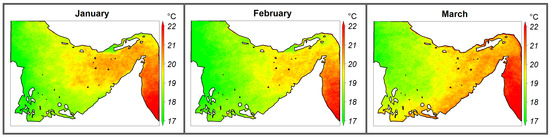
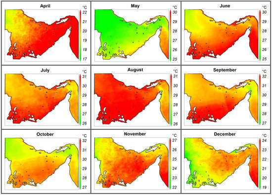
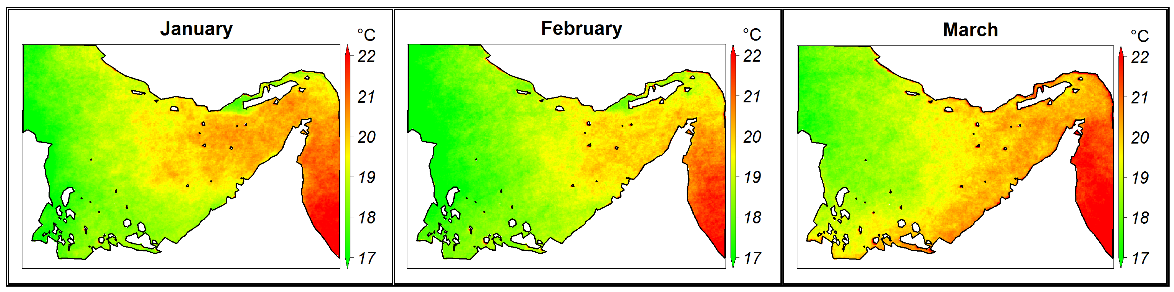
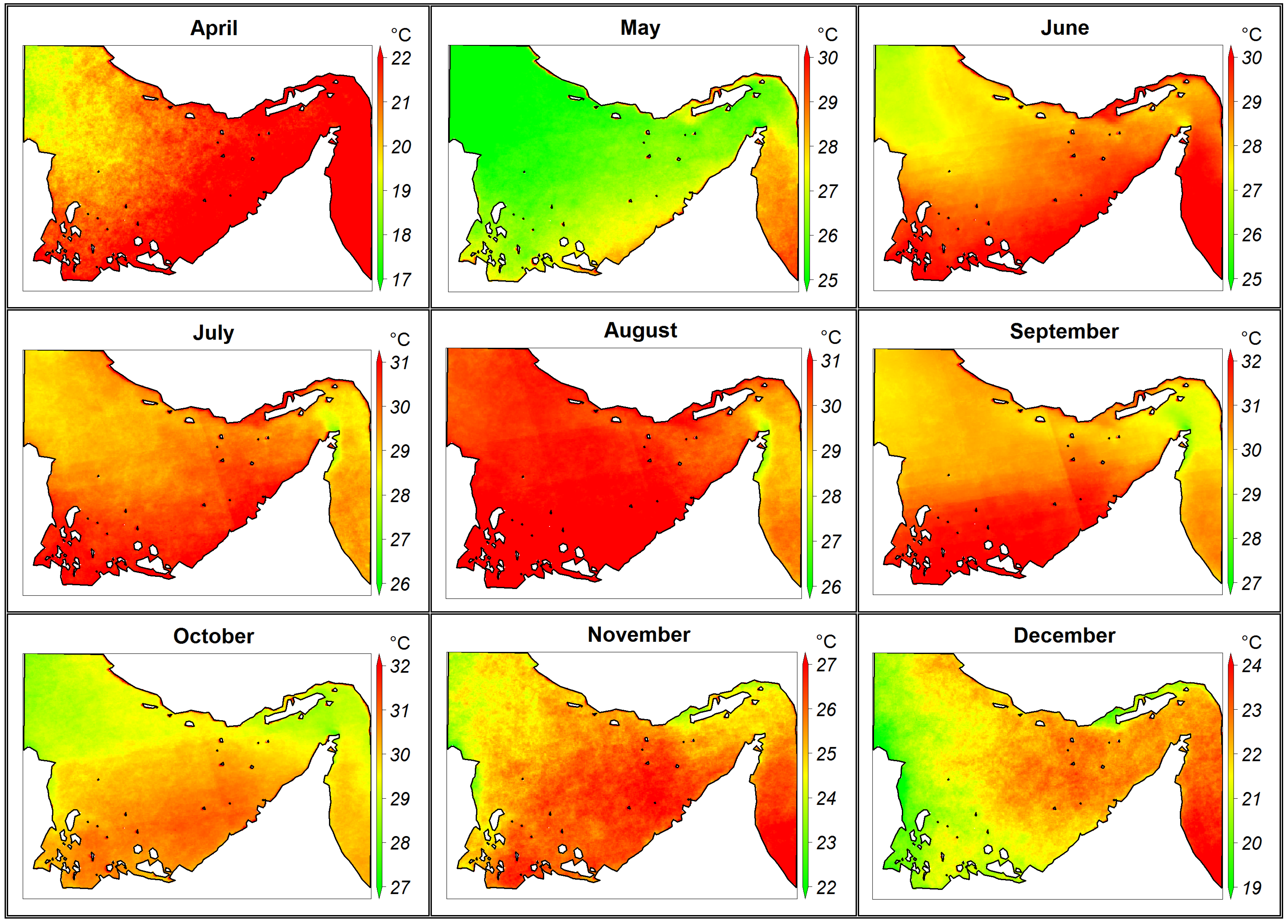
Figure A2.
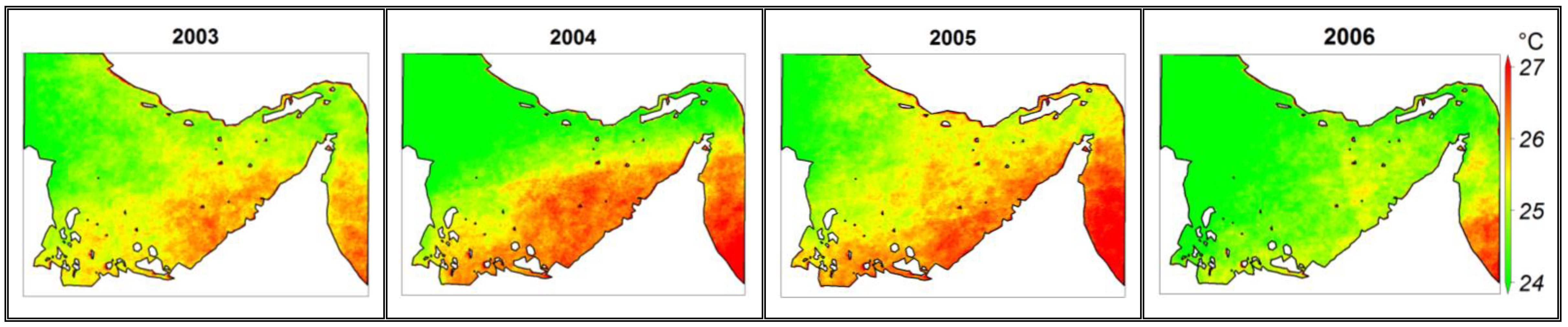
The spatial distribution of the average monthly sea surface temperature (SST) across the Arabian and Oman Gulfs (N.B. the color bar scale varies from figure to figure).
Figure A2.
The spatial distribution of the average monthly sea surface temperature (SST) across the Arabian and Oman Gulfs (N.B. the color bar scale varies from figure to figure).
Appendix C

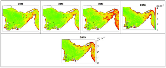
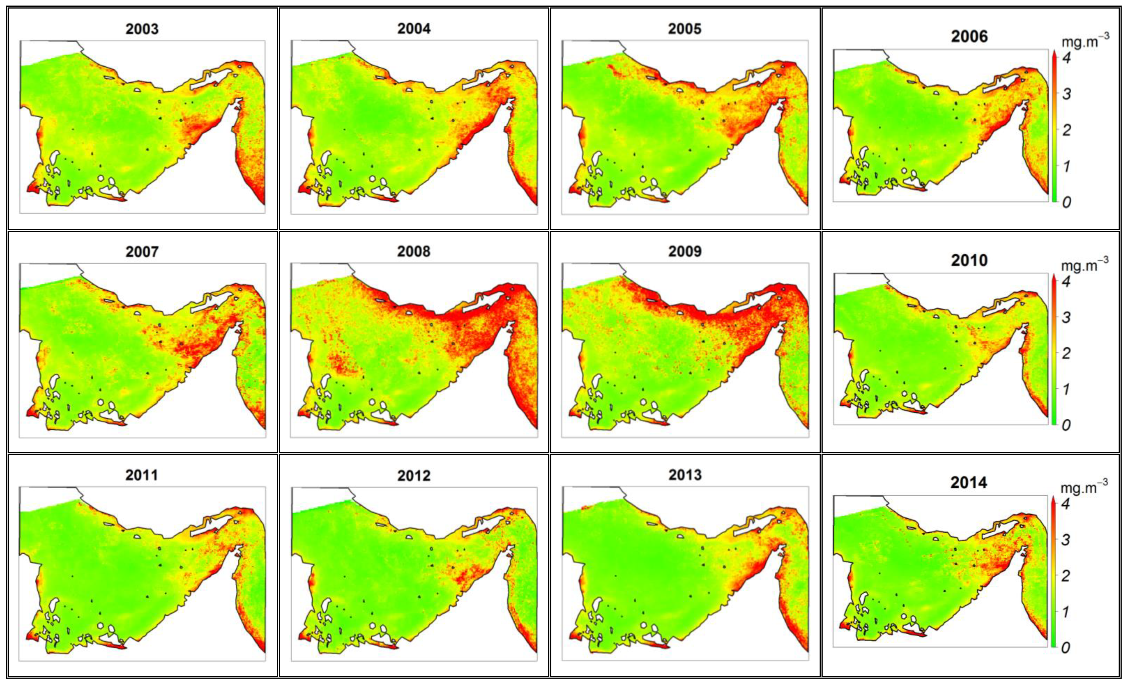
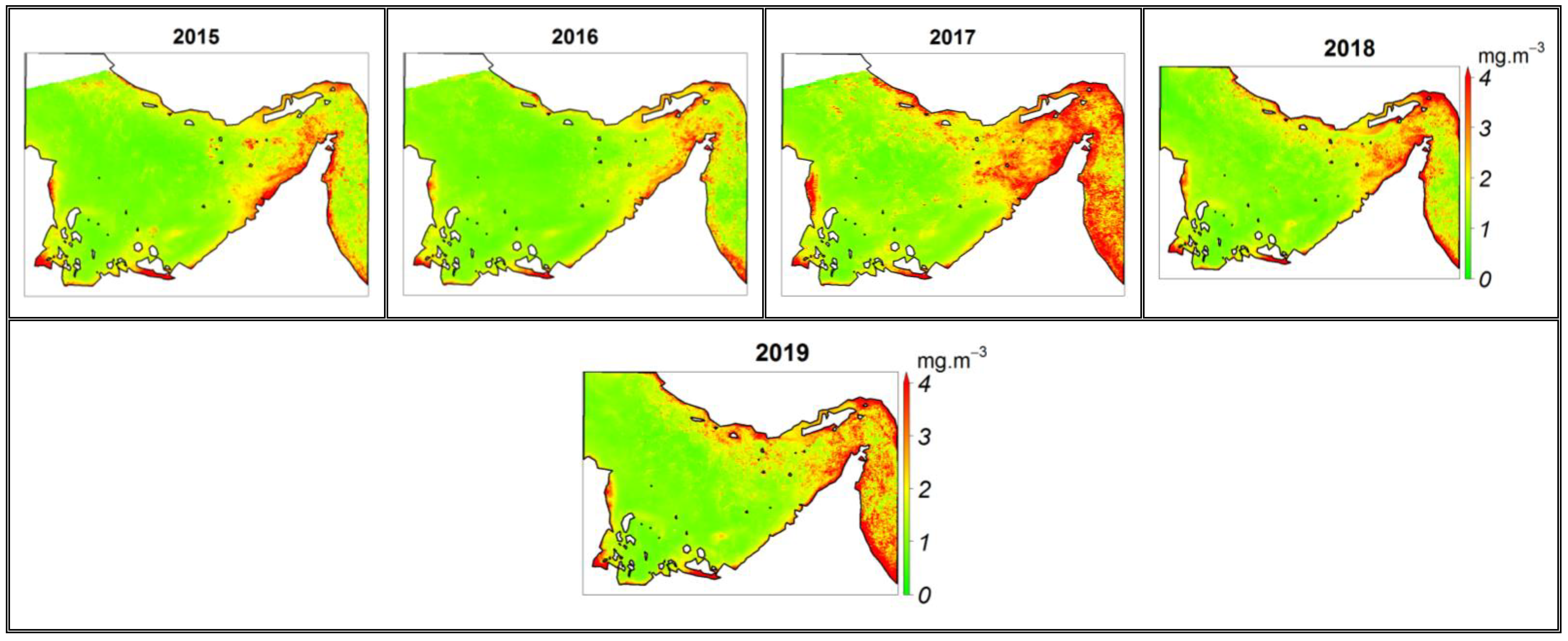
Figure A3.
The spatial distribution of the annual average Chl-a concentration across the Arabian and Oman Gulfs.
Figure A3.
The spatial distribution of the annual average Chl-a concentration across the Arabian and Oman Gulfs.
Appendix D
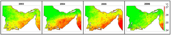
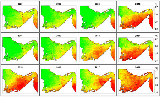

Figure A4.
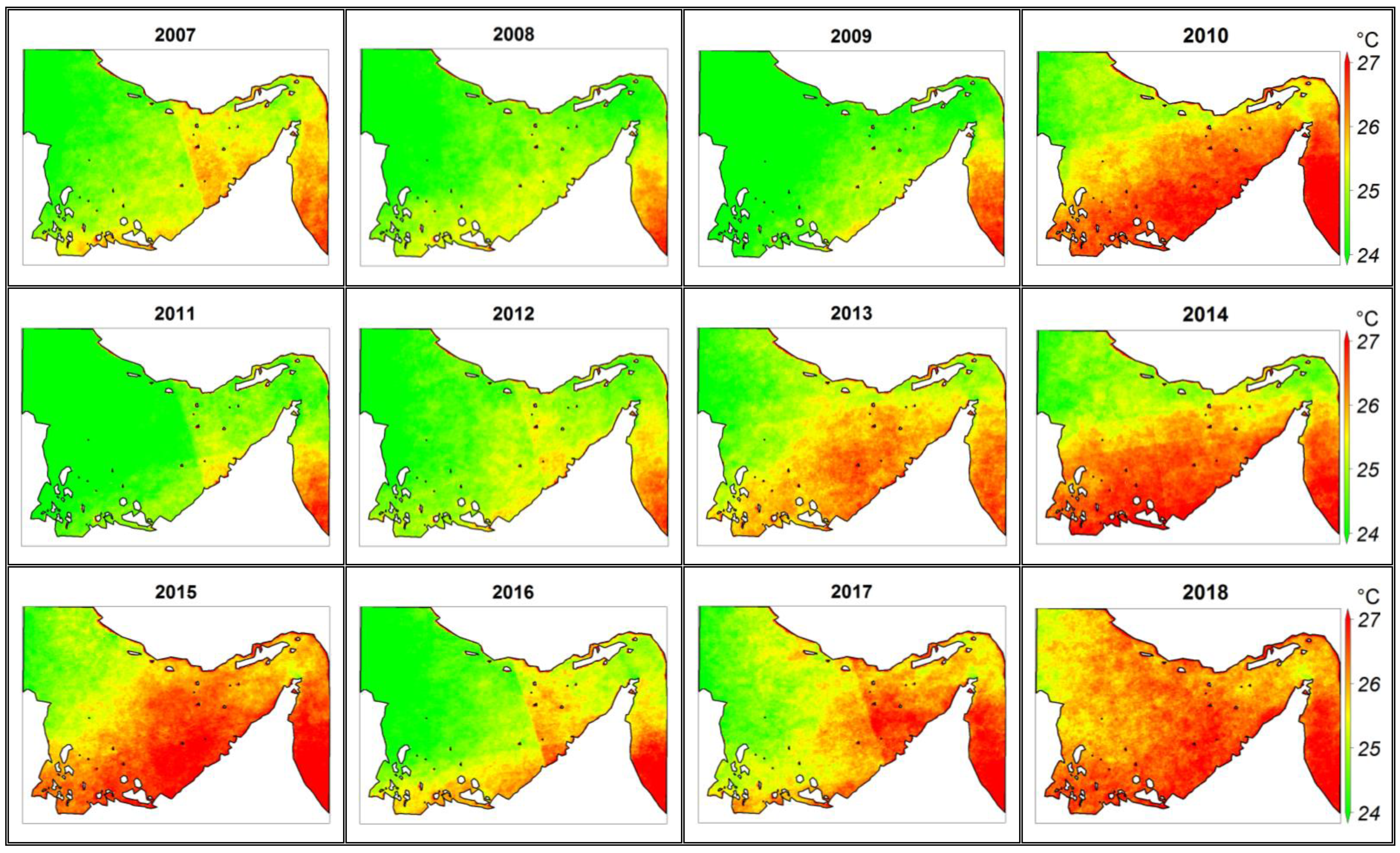
The spatial distribution of the annual average SST across the Arabian and Oman Gulfs.
Figure A4.
The spatial distribution of the annual average SST across the Arabian and Oman Gulfs.

References
- Al Shehhi, M.R.; Gherboudj, I.; Ghedira, H. An overview of historical harmful algae blooms outbreaks in the Arabian Seas. Mar. Pollut. Bull. 2014, 86, 314–324. [Google Scholar] [CrossRef]
- do Rosario Gomes, H.; Goes, J.I.; Matondkar, S.P.; Parab, S.G.; Al-Azri, A.R.; Thoppil, P.G. Blooms of Noctiluca miliaris in the Arabian Sea—An in situ and satellite study. Deep. Sea Res. Part I Oceanogr. Res. Pap. 2008, 55, 751–765. [Google Scholar] [CrossRef]
- Zhao, J.; Ghedira, H. Monitoring red tide with satellite imagery and numerical models: A case study in the Arabian Gulf. Mar. Pollut. Bull. 2014, 79, 305–313. [Google Scholar] [CrossRef]
- Sastry, J.; d’Souza, R. Upwelling and upward mixing in the Arabian Sea. Indian J. Geo Mar. Sci. 1972, 1, 17–27. [Google Scholar]
- Wiggert, J.; Jones, B.; Dickey, T.; Brink, K.; Weller, R.; Marra, J.; Codispoti, L. The Northeast Monsoon’s impact on mixing, phytoplankton biomass and nutrient cycling in the Arabian Sea. Deep. Sea Res. Part II Top. Stud. Oceanogr. 2000, 47, 1353–1385. [Google Scholar] [CrossRef]
- Barzandeh, A.; Eshghi, N.; Hosseinibalam, F.; Hassanzadeh, S. Wind-driven coastal upwelling along the northern shoreline of the Persian Gulf. Boll. Geofis. Teor. Appl. 2018, 59, 301–312. [Google Scholar]
- Chaichitehrani, N.; Allahdadi, M.N. Overview of wind climatology for the Gulf of Oman and the northern Arabian Sea. Am. J. Fluid Dyn. 2018, 8, 1–9. [Google Scholar]
- Banse, K. Seasonality of phytoplankton chlorophyll in the central and northern Arabian Sea. Deep Sea Res. Part A Oceanogr. Res. Pap. 1987, 34, 713–723. [Google Scholar] [CrossRef]
- Kumar, S.P.; Ramaiah, N.; Gauns, M.; Sarma, V.V.S.S.; Muraleedharan, P.M.; Raghukumar, S.; Dileep Kumar, M.; Madhupratap, M. Physical forcing of biological productivity in the Northern Arabian Sea during the Northeast Monsoon. Deep Sea Res. Part II Top. Stud. Oceanogr. 2001, 48, 1115–1126. [Google Scholar] [CrossRef]
- Banse, K.; English, D.C. Comparing phytoplankton seasonality in the eastern and western subarctic Pacific and the western Bering Sea. Prog. Oceanogr. 1999, 43, 235–288. [Google Scholar] [CrossRef]
- Palanisamy, S.; Ahn, Y.-H.; Ryu, J.-H.; Moon, J.-E. Application of optical remote sensing imagery for detection of red tide algal blooms in Korean waters. In Proceedings of the 2005 IEEE International Geoscience and Remote Sensing Symposium—IGARSS’05, Seoul, Korea, 25–29 July 2005; IEEE: New York, NY, USA, 2005. [Google Scholar]
- Blondeau-Patissier, D.; Gower, J.F.; Dekker, A.G.; Phinn, S.R.; Brando, V.E. A review of ocean color remote sensing methods and statistical techniques for the detection, mapping and analysis of phytoplankton blooms in coastal and open oceans. Prog. Oceanogr. 2014, 123, 123–144. [Google Scholar] [CrossRef] [Green Version]
- Prigent, C.; Aires, F.; Rossow, W.B. Land surface skin temperatures from a combined analysis of microwave and infrared satellite observations for an all-weather evaluation of the differences between air and skin temperatures. J. Geophys. Res. Atmos. 2003, 108. [Google Scholar] [CrossRef]
- Miles, T.; He, R. Seasonal surface ocean temporal and spatial variability of the South Atlantic Bight: Revisiting with MODIS SST and Chl-a imagery. Cont. Shelf Res. 2010, 30, 1951–1962. [Google Scholar] [CrossRef]
- Alvera-Azcárate, A.; Barth, A.; Beckers, J.M.; Weisberg, R.H. Multivariate reconstruction of missing data in sea surface temperature, chlorophyll, and wind satellite fields. J. Geophys. Res. Oceans 2007, 112. [Google Scholar] [CrossRef] [Green Version]
- Petchprayoon, P. Analysis of Climate Change Impacts on Surface Energy Balance of Lake Huron (Estimation of Surface Energy Balance Components: Remote Sensing Approach for Water–Atmosphere Parameterization); University of Colorado at Boulder: Boulder, CO, USA, 2015. [Google Scholar]
- Brewin, R.J.; Raitsos, D.E.; Pradhan, Y.; Hoteit, I. Comparison of chlorophyll in the Red Sea derived from MODIS-Aqua and in vivo fluorescence. Remote Sens. Environ. 2013, 136, 218–224. [Google Scholar] [CrossRef]
- Hu, C.; Lee, Z.; Franz, B. Chlorophyll aalgorithms for oligotrophic oceans: A novel approach based on three-band reflectance difference. J. Geophys. Res. Oceans 2012, 117. [Google Scholar] [CrossRef] [Green Version]
- Nezlin, N.P.; Kostianoy, A.G.; Grégoire, M. Patterns of seasonal and interannual changes of surface chlorophyll concentration in the Black Sea revealed from the remote sensed data. Remote Sens. Environ. 1999, 69, 43–55. [Google Scholar] [CrossRef]
- Tang, D.-L.; Ni, I.-H.; Kester, D.R.; Müller-Karger, F.E. Remote sensing observations of winter phytoplankton blooms southwest of the Luzon Strait in the South China Sea. Mar. Ecol. Prog. Ser. 1999, 191, 43–51. [Google Scholar] [CrossRef] [Green Version]
- Gurlin, D.; Gitelson, A.A.; Moses, W.J. Remote estimation of chl-a concentration in turbid productive waters—Return to a simple two-band NIR-red model? Remote Sens. Environ. 2011, 115, 3479–3490. [Google Scholar] [CrossRef]
- Gower, J.F.; King, S.A. Distribution of floating Sargassum in the Gulf of Mexico and the Atlantic Ocean mapped using MERIS. Int. J. Remote Sens. 2011, 32, 1917–1929. [Google Scholar] [CrossRef]
- Gower, J.; King, S.; Goncalves, P. Global monitoring of plankton blooms using MERIS MCI. Int. J. Remote Sens. 2008, 29, 6209–6216. [Google Scholar] [CrossRef]
- Cannizzaro, J.P.; Carder, K.L.; Chen, F.R.; Heil, C.A.; Vargo, G.A. A novel technique for detection of the toxic dinoflagellate, Karenia brevis, in the Gulf of Mexico from remotely sensed ocean color data. Cont. Shelf Res. 2008, 28, 137–158. [Google Scholar] [CrossRef]
- Hu, C.; Lee, Z.; Ma, R.; Yu, K.; Li, D.; Shang, S. Moderate resolution imaging spectroradiometer (MODIS) observations of cyanobacteria blooms in Taihu Lake, China. J. Geophys. Res. Oceans 2010, 115. [Google Scholar] [CrossRef] [Green Version]
- Anderson, C.R.; Kudela, R.M.; Burrell, C.T.; Langlois, G.; Goodman, J.; Benitez-Nelson, C.; Sekula-Wood, E.; Chao, Y.; Siegel, D.A. Detecting toxic diatom blooms from ocean color and a regional ocean model. Geophys. Res. Lett. 2011, 38. [Google Scholar] [CrossRef] [Green Version]
- Kavak, M.T.; Karadogan, S. The relationship between sea surface temperature and chlorophyll concentration of phytoplanktons in the Black Sea using remote sensing techniques. J. Environ. Biol. 2012, 33, 493. [Google Scholar] [PubMed]
- Nurdin, S.; Mustapha, M.A.; Lihan, T. The relationship between sea surface temperature and chlorophyll-a concentration in fisheries aggregation area in the archipelagic waters of Spermonde using satellite images. In AIP Conference Proceedings; American Institute of Physics: New York, NY, USA, 2013. [Google Scholar]
- Jutla, A.S.; Akanda, A.S.; Griffiths, J.K.; Colwell, R.; Islam, S. Warming oceans, phytoplankton, and river discharge: Implications for cholera outbreaks. Am. J. Trop. Med. Hyg. 2011, 85, 303–308. [Google Scholar] [CrossRef] [PubMed] [Green Version]
- Kouketsu, S.; Kaneko, H.; Okunishi, T.; Sasaoka, K.; Itoh, S.; Inoue, R.; Ueno, H. Mesoscale eddy effects on temporal variability of surface chlorophyll a in the Kuroshio Extension. J. Oceanogr. 2016, 72, 439–451. [Google Scholar] [CrossRef]
- Chu, P.C.; Kuo, Y.-H. Biophysical variability in the Kuroshio Extension from Altimeter and SeaWiFS. In Proceedings of the OCEANS 2009, Biloxi, MS, USA, 26–29 October 2009; IEEE: New York, NY, USA, 2009. [Google Scholar]
- Emery, K.O. Sediments and water of Persian Gulf. AAPG Bull. 1956, 40, 2354–2383. [Google Scholar]
- Vaughan, G.O.; Al-Mansoori, N.; Burt, J.A. The arabian gulf. In World Seas: An Environmental Evaluation; Elsevier: Amsterdam, The Netherlands, 2019; pp. 1–23. [Google Scholar]
- The Editors of Encyclopaedia Britannica. Gulf of Oman. In Encyclopedia Britannica. 2020. Available online: https://www.britannica.com/place/Gulf-of-Oman (accessed on 9 March 2021).
- Al Senafi, F.; Anis, A. Shamals and climate variability in the Northern Arabian/Persian Gulf from 1973 to 2012. Int. J. Climatol. 2015, 35, 4509–4528. [Google Scholar] [CrossRef]
- Nezlin, N.P.; Polikarpov, I.G.; Al-Yamani, F.Y.; Rao, D.S.; Ignatov, A.M. Satellite monitoring of climatic factors regulating phytoplankton variability in the Arabian (Persian) Gulf. J. Mar. Syst. 2010, 82, 47–60. [Google Scholar] [CrossRef]
- Noori, R.; Tian, F.; Berndtsson, R.; Abbasi, M.R.; Naseh, M.V.; Modabberi, A.; Soltani, A.; Kløve, B. Recent and future trends in sea surface temperature across the Persian Gulf and Gulf of Oman. PLoS ONE 2019, 14, e0212790. [Google Scholar] [CrossRef]
- Dwyer, J.; Schmidt, G. The MODIS reprojection tool. In Earth Science Satellite Remote Sensing; Springer: Berlin/Heidelberg, Germany, 2006; pp. 162–177. [Google Scholar]
- Moradi, M.; Kabiri, K. Spatio-temporal variability of SST and Chlorophyll-a from MODIS data in the Persian Gulf. Mar. Pollut. Bull. 2015, 98, 14–25. [Google Scholar] [CrossRef] [PubMed]
- Wan, Z. MODIS Land-Surface Temperature Algorithm Theoretical Basis Document (LST ATBD); Institute for Computational Earth System Science: Santa Barbara, CA, USA, 1999; Volume 75. [Google Scholar]
- Crosman, E.T.; Horel, J.D. MODIS-derived surface temperature of the Great Salt Lake. Remote Sens. Environ. 2009, 113, 73–81. [Google Scholar] [CrossRef]
- Hereher, M.E. Assessment of climate change impacts on sea surface temperatures and sea level rise—The Arabian Gulf. Climate 2020, 8, 50. [Google Scholar] [CrossRef] [Green Version]
- Oesch, D.; Jaquet, J.M.; Klaus, R.; Schenker, P. Multi-scale thermal pattern monitoring of a large lake (Lake Geneva) using a multi-sensor approach. Int. J. Remote Sens. 2008, 29, 5785–5808. [Google Scholar] [CrossRef] [Green Version]
- Oesch, D.C.; Jaquet, J.M.; Hauser, A.; Wunderle, S. Lake surface water temperature retrieval using advanced very high resolution radiometer and Moderate Resolution Imaging Spectroradiometer data: Validation and feasibility study. J. Geophys. Res. Oceans 2005, 110. [Google Scholar] [CrossRef] [Green Version]
- Reinart, A.; Reinhold, M. Mapping surface temperature in large lakes with MODIS data. Remote Sens. Environ. 2008, 112, 603–611. [Google Scholar] [CrossRef]
- Amante, C.; Eakins, B.W. ETOPO1 Arc-Minute Global Relief Model: Procedures, Data Sources and Analysis; National Geophysical Data Center: Boulder, CO, USA, 2009; Volume 10, p. V5C8276M. [Google Scholar]
- Li, Y.; He, R. Spatial and temporal variability of SST and ocean color in the Gulf of Maine based on cloud-free SST and chlorophyll reconstructions in 2003–2012. Remote Sens. Environ. 2014, 144, 98–108. [Google Scholar] [CrossRef]
- Monahan, A.H.; Fyfe, J.C.; Ambaum, M.H.; Stephenson, D.B.; North, G.R. Empirical orthogonal functions: The medium is the message. J. Clim. 2009, 22, 6501–6514. [Google Scholar] [CrossRef] [Green Version]
- Wikle, C.K.; Zammit-Mangion, A.; Cressie, N. Spatio-Temporal Statistics with R; CRC Press: Boca Raton, FL, USA, 2019. [Google Scholar]
- Pearson, K., VII. Note on regression and inheritance in the case of two parents. Proc. R. Soc. Lond. 1895, 58, 240–242. [Google Scholar]
- Hirsch, R.M.; Slack, J.R.; Smith, R.A. Techniques of trend analysis for monthly water quality data. Water Resour. Res. 1982, 18, 107–121. [Google Scholar] [CrossRef] [Green Version]
- Libiseller, C.; Grimvall, A. Performance of partial Mann–Kendall tests for trend detection in the presence of covariates. Environ. Off. J. Int. Environ. Soc. 2002, 13, 71–84. [Google Scholar] [CrossRef]
- Nezlin, N.P.; Polikarpov, I.G.; Al-Yamani, F. Satellite-measured chlorophyll distribution in the Arabian Gulf: Spatial, seasonal and inter-annual variability. Int. J. Oceans Oceanogr. 2007, 2, 139–156. [Google Scholar]
- Richlen, M.L.; Morton, S.L.; Jamali, E.A.; Rajan, A.; Anderson, D.M. The catastrophic 2008–2009 red tide in the Arabian gulf region, with observations on the identification and phylogeny of the fish-killing dinoflagellate Cochlodinium polykrikoides. Harmful Algae 2010, 9, 163–172. [Google Scholar] [CrossRef]
- Prasad, T.; Ikeda, M. A numerical study of the seasonal variability of Arabian Sea high-salinity water. J. Geophys. Res. Oceans 2002, 107, 18-1–18-12. [Google Scholar] [CrossRef]
- Nandkeolyar, N.; Raman, M.; Kiran, G.S. Comparative analysis of sea surface temperature pattern in the eastern and western gulfs of Arabian Sea and the Red Sea in recent past using satellite data. Int. J. Oceanogr. 2013, 2013, 501602. [Google Scholar] [CrossRef]
- Björnsson, H.; Venegas, S. A manual for EOF and SVD analyses of climatic data. CCGCR Rep. 1997, 97, 112–134. [Google Scholar]
- Piontkovski, S.; Chiffings, T. Long-term changes of temperature in the Sea of Oman and the western Arabian Sea. Int. J. Oceans Oceanogr. 2014, 8, 53–72. [Google Scholar]


Publisher’s Note: MDPI stays neutral with regard to jurisdictional claims in published maps and institutional affiliations. |
© 2021 by the authors. Licensee MDPI, Basel, Switzerland. This article is an open access article distributed under the terms and conditions of the Creative Commons Attribution (CC BY) license (https://creativecommons.org/licenses/by/4.0/).