Article

Comparison of Machine Learning Methods to Up-Scale Gross Primary Production

1
Research Institute of Forest Resource Information Techniques, Chinese Academy of Forestry, Beijing 100091, China
2
Key Laboratory of Forestry Remote Sensing and Information System, National Forestry and Grassland Administration, Beijing 100091, China
3
State Key Laboratory of Remote Sensing Science, Jointly Sponsored by Beijing Normal University and Institute of Remote Sensing and Digital Earth of Chinese Academy of Sciences, Beijing 100875, China
4
Beijing Engineering Research Center for Global Land Remote Sensing Products, Institute of Remote Sensing Science and Engineering, Faculty of Geographical Science, Beijing Normal University, Beijing 100875, China
*
Author to whom correspondence should be addressed.
These authors contributed equally to this work.
Remote Sens. 2021, 13(13), 2448; https://doi.org/10.3390/rs13132448
Submission received: 24 May 2021 / Revised: 20 June 2021 / Accepted: 22 June 2021 / Published: 23 June 2021
(This article belongs to the Special Issue Recent Advances in Satellite Derived Global Land Product Validation)

Abstract

:
Eddy covariance observation is an applicable way to obtain accurate and continuous carbon flux at flux tower sites, while remote sensing technology could estimate carbon exchange and carbon storage at regional and global scales effectively. However, it is still challenging to up-scale the field-observed carbon flux to a regional scale, due to the heterogeneity and the unstable air conditions at the land surface. In this paper, gross primary production (GPP) from ground eddy covariance systems were up-scaled to a regional scale by using five machine learning methods (Cubist regression tree, random forest, support vector machine, artificial neural network, and deep belief network). Then, the up-scaled GPP were validated using GPP at flux tower sites, weighted GPP in the footprint, and MODIS GPP products. At last, the sensitivity of the input data (normalized difference vegetation index, fractional vegetation cover, shortwave radiation, relative humidity and air temperature) to the precision of up-scaled GPP was analyzed, and the uncertainty of the machine learning methods was discussed. The results of this paper indicated that machine learning methods had a great potential in up-scaling GPP at flux tower sites. The validation of up-scaled GPP, using five machine learning methods, demonstrated that up-scaled GPP using random forest obtained the highest accuracy.

1. Introduction

As vegetation productivity is an important part of the terrestrial carbon cycle, accurately estimating this component is significant in research on terrestrial ecosystems, carbon cycles, and climate change [1,2,3,4]. Gross primary productivity (GPP) is one of the main factors to determine the carbon source and sink of the ecosystems, which could reflect the response of the ecosystems to global change [5]. Ground-observed data are most representative in an area around the field instruments; the area that defined the spatial context of the measurement means footprint scale of the field data [6,7]. Remote sensing technology could monitor the land surface carbon exchange and carbon storage in a large area, which is at a regional or global scale. However, it is still a challenge to match the field data with GPP derived from satellite observations data, and to up-scale GPP at flux tower sites to a regional scale [8]. In this condition, studies to exploit the ways of up-scaling ground-observed GPP to regional GPP, and to validate the effectiveness of these methods, is of great significance in revealing vegetation productivity dynamics and carbon budgets [9].
Studies have been carried out to up-scale GPP at flux tower sites to a regional scale or global scale based on remote sensing data in recent years [10,11,12,13]. Some regression models [12,13,14] have been developed based on the assumption that the relationships between field data and the corresponding satellite image pixels are constant. For example, Jung et al. [15,16] up-scaled FLUXNET carbon data to a global scale, with a resolution of 0.5°, using an integrated regression tree based on the relationship between GPP and fraction of photosynthetically active radiation (FPAR), and validated the results against Moderate Resolution Imaging Spectroradiometer (MODIS) products and GPP, using the Biome bio-geochemical cycle (Biome-BGC) model. Badgley et al. analyzed the relationship between GPP and near-infrared reflectance of vegetation (NIRv) from FLUXNET eddy covariance sites, and estimated the global annual terrestrial photosynthesis [10]. Virkkala et al. up-scaled CO2 fluxes at a relatively high spatial resolution (1 km2) across the high-latitude region, using five commonly used statistical models [17]. Gu et al. [18] described a relationship between the satellite-derived growing season averaged normalized difference vegetation index (NDVI) and annual productivity for grasslands in the Greater Platte River Basin of the United States. Gilmanov et al. [19] studied long-term measurements at five Northern Great Plains to obtain relationships between carbon dioxide fluxes and photosynthetically active radiation.
However, studies have also indicated that the regression models based on the relationship between GPP at flux tower sites and other variables (such as field FPAR, vegetation index) had poor robustness when up-scaling to a regional scale [12,13,20]. To solve this problem, some machine learning models, such as the regression tree [21], artificial neural network (ANN) [22], random forest (RF) [23,24,25], and support vector machine (SVM) [26], have been used to retrieve the land surface parameters from remote sensing data. Although the eco-physiological processes of the machine learning models were not clear, and the accuracy relied much on the number and representativeness of the training data. Some researches tried to up-scale GPP from the perspective of data assimilation, which could make the best of the observed data and prior knowledge of the parameters. For example, Desai et al. used the Markov chain Monte Carlo (MCMC) model to up-scale carbon flux data [27]. Xiao et al. up-scaled GPP in the Northern United States, using the diagnostic carbon flux model (DCFM), based on the data assimilation from 17 flux net stations [28]. Chen et al. optimized the parameters of the vegetation photosynthesis model (VPM) to derive GPP from an assimilation of footprint and Landsat data [29]. However, the data assimilation usually occupies a large amount of computation. Some other studies tried to up-scale the inputs of the GPP model firstly, then estimated the regional GPP by using the up-scaled inputs [30,31], but the errors of the input data in the up-scaling process would have an influence on the accuracy of the results, and the uncertainty was difficult to qualify. To sum up, although some up-scaling methods of GPP, using statistical regression, data assimilation and machine learning models, have been proposed in recent years, few studies focused on the difference in the accuracy and feasibility these up-scaled models. In this condition, comparing the precision of these methods and analyzing the applicability of these models is urgent.
It is an effective way to validate the estimated GPP by comparison with the observed data. The flux net observed network, such as FLUXNET, AmeriFLUX, AsiaFLUX, ChinaFLUX, which contained more than 500 total stations, had been constructed to monitor carbon flux regionally or globally, and to validate the simulative GPP from different kinds of models [32,33,34]. Some other projects, such as Validation of Land European Remote Sensing Instruments (VALERI) [35] and BigFoot [36,37], had also been designed to validate the satellite products. Considering the difference in the footprint between field observed data and the satellite data would bring some uncertainty in direct validation; some indirect validation methods were also proposed to assess the precision of the remote sensing products. For example, Wang et al. validated the estimated biomass and Net Primary Production (NPP) with field data firstly, then up-scaled NPP to 1 km and validated the estimated NPP at a regional scale [38]. Mueller et al. found that the difference in the estimated annual average global GPP could be as high as 50% when validating from field data to regional data [39]. The validation of up-scaled GPP had typically been on training (flux tower) sites, which are limited in number and mostly not independent. Few studies concentrated on the validation of scale transform results at different scales systematically. In this case, studying the validating methods of up-scaled GPP at several scales is of great significance.
The aims of this paper are to up-scale GPP at flux tower sites to a regional scale, by using five machine learning models (Cubist regression tree, RF, SVM, ANN and deep belief network (DBN)), based on remote sensing data (MODIS land surface reflectance products, and derived fractional vegetation cover, land-cover products), and to compare the accuracy of the different up-scaling approaches. The results of this paper demonstrated the applicability and feasibility of machine learning models in up-scaling GPP at flux tower sites.

2. Materials and Methods
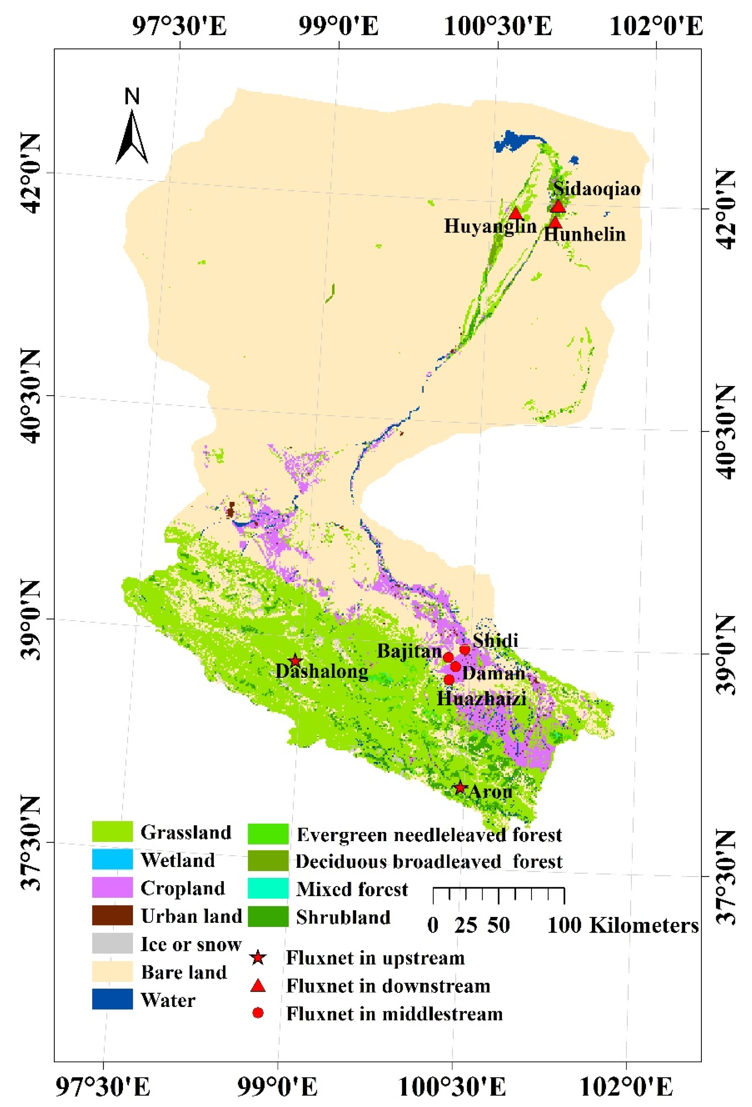
2.1. Study Area

A case study was conducted in Heihe River Basin, which is located in an arid and semi-arid area in Northwestern China (37°41′~42°42′N, 96°42′~102°00′E), and could be divided into upper basin, mid-basin and lower basin generally according to the natural, ecological and climate characteristics [40]. Land-cover types in this area include deciduous broadleaved forest (DBF), evergreen needle-leaved forest (ENF), mixed forest (MF), cropland, bare land, wetland, shrub land, grass land, water, ice or snow (Figure 1). Bare lands are mainly distributed in the downstream in the northern areas, forest and cropland constitute the dominant lands in the upstream in southern areas. Additionally, some shrub lands and wetlands are also distributed in the southern areas. The study area could be divided into mainly bare land in the north with an elevation range from 500 m to 1000 m, and mountains in the south with an elevation about 1000 m~5500 m. This area has a temperate climate, with an average annual air temperature about 6.0~8.0 °C, an average annual precipitation about 100~250 mm, and an average annual pan evaporation about 1200~1800 mm [41,42].

2.2. Data and Data Processing

2.2.1. Remote Sensing Data

A. MODIS Land Surface Reflectance Products

The MODIS land surface reflectance (LSR) products (MOD09A1) with a spatial resolution of 500 m were provided on an 8-day basis [43]. In this study, MODIS LSR products from May to September in 2014 were used. These data contained the best possible observation during an 8-day period after atmospheric correction, which could provide an estimate of the surface reflectance as it would be measured at ground level in the absence of atmospheric scattering or absorption [44]. Then 8-day NDVI were derived using the red and near-infrared reflectance from LSR products, and were aggregated to 1 km to train the up-scaling model of GPP. Additionally, 8-day fractional vegetation cover (FVC) from May to September in 2014 were also obtained from 8-day NDVI by using the dimidiate pixel model [45], and were also aggregated to 1 km.

B. Land-Cover Products

The land-cover map, which comprised of 11 land-cover types, including forests, crops, bare lands and wetlands with a spatial resolution of 30 m and temporal resolution of one month in 2014 was adopted in this paper [46]. This map was generated from Chinese HJ-1 satellite images based on the time-series patterns of the land-cover types [47,48]. Studies have shown that the overall classification accuracy of the map could be as high as 92.19% [49]. To make the datasets comparable, the 30 m land-cover data were aggregated to 1 km.

C. MODIS GPP Products

The MODIS primary production products (MOD17A2) were designed to provide an accurate regular measure of the growth of the terrestrial vegetation with a spatial resolution of 1 km and temporal resolution of 8 days [50]. MOD17 GPP outputs, which were generated using a radiation use efficiency model, were useful for global carbon cycle analysis, ecosystem status assessment, and environmental change monitoring. Modification of parameters in the Biome property look-up table (BPLUT) had been made to agree with GPP derived from measurements at eddy flux towers and estimated GPP [51]. The BPLUT contains parameters for temperature and vapor pressure difference (VPD) limits, light use efficiency, specific leaf area and respiration coefficients for representative vegetation in each biome type [51]. In this study, MODIS GPP products from May to September in 2014 were used as the reference data to cross validate the up-scaling results.

2.2.2. Meteorological Data

Meteorological datasets, including air pressure, precipitation, wind speed and direction, air temperature and humidity, and four radiation components (upward shortwave radiation, downward shortwave radiation, upward longwave radiation, downward longwave radiation) were collected from nine automatic meteorological stations in the study area from May to September in 2014. Meteorological observation instruments were installed at the flux towers (Figure 1), so the meteorological observations were also taken at the flux tower sites. Average values were obtained every 30 min from the observed every 10 min data. Meteorological datasets from meteorological stations were used to calculate the real time (every 30 min) footprint of the flux data.
Datasets of 2 m surface vapor pressure, vapor-to-liquid ratio, downward shortwave radiation and the precipitation were generated with a spatial resolution of 0.05°, and temporal resolution of one hour from the weather research and forecasting model (WRF) from May to September in 2014 were also collected [52]. Studies have demonstrated that a good linear relationship (R2 was higher than 0.90) existed between the datasets and the observed data from China Meteorological Administration and seven Watershed Allied Telemetry Experimental Research (WATER) stations [53,54]. These datasets (2 m surface vapor pressure, vapor-to-liquid ratio, downward shortwave radiation and the precipitation) were interpolated to 1 km firstly, then were used to up-scale GPP from flux tower sites to regional scale.

2.2.3. Field Data

Field carbon flux data used in this study were derived from the Multi-Scale Observation Experiment on Evapotranspiration over heterogeneous land surfaces in 2012 of the Heihe Watershed Allied Telemetry Experiment Research (HiWATER-MUSOEXE) [54,55,56]. Half-hourly carbon flux data from 2 eddy covariance systems in the upstream, 4 eddy covariance systems in the midstream and 3 eddy covariance systems in the downstream (Table 1) were collected. Time period of the flux data was from May to September in 2014. Land-cover types of the 9 eddy covariance systems included cropland (mainly maize), bare land, grass land, shrub land, wetland, and forest. Gaps in the observed datasets, which were caused by the system malfunction, wind and rain were firstly filled. Principles to control data quality and to exclude the outlier of the datasets were as follows: (1) excluding the observed data one hour before and after precipitation; (2) excluding the data that were outside the instruments’ measurement range or outside the reasonable range of values; (3) excluding the negative value at night due to there being no assimilation of carbon dioxide in the photosynthesize at night; (4) excluding the datasets when friction velocities were lower than the threshold value [57,58,59] at night.
At daytime, gaps in the flux data were filled by using a look-up table [58,59], which was built on flux, air temperature and photosynthetically active radiation. At night, gaps in the flux data were filled based on the relationship between the ecosystem respiration and the air temperature or the soil temperature, which was described as [59] follows:
R e c o = a e b T
where R e c o is ecosystem respiration (mg∙m−2∙s−1), a and b are the coefficient, T is the air temperature or the soil temperature (°C) at night.
Then daily carbon flux was obtained by summing the half-hourly carbon flux data. At last, daily GPP were obtained by partitioning the observed net flux into GPP and ecosystem respiration [59,60,61], the process could be described as [59,60,61] follows:
GPP = R e c o NEE
where NEE is the net ecosystem carbon dioxide exchange. One advantage of using daily data instead of half-hourly intervals to derive daily GPP is to reduce errors on deriving NEE and GPP using temperature and radiation, because observed fluxes and meteorological conditions such as photosynthetic active radiation have significant variations from hour-to-hour [62,63]. Studies indicated that using daily data could reduce the effect of the hour-to-hour variations when deriving NEE and GPP [62,63].

2.3. Methods

The flowchart of up-scaling GPP using machine learning method is shown in Figure 2. Firstly, the GPP from eddy covariance systems were up-scaled based on the MODIS NDVI, land-cover types, FVC and the meteorological datasets using five machine learning methods (Cubist regression tree, RF, SVM, ANN, DBN). A footprint source area model (FSAM) [64,65,66,67] was adopted to obtain the footprint of GPP at flux tower sites used in this study. Then the up-scaled GPP were validated at in situ scale, at footprint scale and at regional scale. At last, up-scaling GPP using different machine learning methods were compared, sensitiveness of the input data to the up-scaled GPP was analyzed, and the uncertainty of the methods was discussed.

2.3.1. Up-Scaling GPP Using Machine Learning Methods

Studies have shown that GPP is influenced by shortwave radiation (SWR), air temperature (Ta), vapor pressure deficit (VPD), soil moisture and nitrogen availability at canopy scale. While at ecosystem scale, GPP was well related to leaf area index (LAI), NDVI and canopy phenology [68]. In this paper, NDVI and FVC, which were selected as two of the inputs to describe the terrestrial photosynthetic vegetation activity to train the machine learning models to up-scale GPP at flux tower sites. Moreover, considering that SWR, Ta and RH characterized the condition of carbon storage under natural environment [9,69], these factors were also taken into account when up-scaling GPP at flux tower sites. Daily GPP from the field carbon flux data, and corresponding remote sensing data (NDVI, FVC, land cover) and meteorological data (SWR, Ta, RH) were selected as the training datasets of machine learning methods. To make the input parameters comparable, the inputs of the training data were normalized firstly. Then five machine learning methods (Cubist regression tree [70,71], RF [72], SVM [26], ANN [73], DBN [74]) were adopted to up-scale the GPP at flux tower sites.

2.3.2. Footprint of GPP at Flux Tower Sites

To analyze the spatial representativeness of GPP from ground eddy covariance systems, FSAM [64,65,66,67] was adopted to study the real-time footprint of GPP at flux tower sites. FSAM was a two-dimensional advection diffusion equation based on the K-theory and the analysis of advection diffusion. Inputs of FSAM included friction velocity ( u ), Obukhov length (L), standard deviation of cross wind velocity fluctuations ( δ v ), measurement height (zm), zero-plane displacement height ( z d ) and surface roughness length ( z 0 ). We used the meteorological datasets (air pressure, precipitation, wind speed and direction, air temperature and humidity, upward shortwave radiation, downward shortwave radiation, upward longwave radiation, downward longwave radiation) from the automatic meteorological stations to run FSAM and to obtain the near real-time (every 30 min) footprint of the observed data. Then a weighted model was used to calculate the climate footprint (footprint in the growing season from May to September) of GPP in 2014, and the model was described as follows:
f c l i m a t o l o g y ( x , y , z m ) = i = 1 N f ( x , y , z m ) F l u x ( i ) F l u x ( i )
where i is the step (30 min), N is the number of 30-min intervals of observed GPP in the time step, (x,y) is the location of ground-level point sources, x is in the up-wind direction, and y is in the cross wind direction, f c l i m a t o l o g y ( x , y , z m ) is the climate footprint of GPP, f ( x , y , z m ) is the real-time footprint of GPP, F l u x ( i ) is the observed GPP from ground eddy covariance systems.

2.3.3. Validation of Up-Scaled GPP

To assess the performance of the up-scaling GPP using machine learning methods, the up-scaled GPP were validated using GPP at flux tower sites, using weighted GPP in the footprint, and were compared with MODIS GPP products. The determination coefficient (R2) and root mean square error (RMSE) were used to quantify the accuracy of the results.
Firstly, up-scaled GPP pixels were directly compared with corresponding GPP derived from ground eddy covariance systems. Moreover, time series (from May to September in 2014) of up-scaled GPP and GPP at flux tower sites were compared.
Additionally, pixels in the footprint were selected as the validation pixels. Then the GPP at flux tower sites were weighted average in the footprint and were compared with corresponding up-scaled GPP pixels from five machine learning methods. In theory, the footprint of GPP from ground eddy covariance systems is infinite, as the ground-observed flux is the total integral of over an infinite region in the windward direction. In this paper, a 6 km × 6 km area was used to compare the GPP at flux tower sites in the footprint and corresponding up-scaled GPP results. The weight of GPP at flux tower sites in the footprint was calculated by the following:
R = f ( x , y , z m ) i i = 1 N f ( x , y , z m ) i × 100 %
where R is the weight of the pixel, f ( x , y , z m ) i is the footprint of i-th pixel, N is the total number of the pixels.
At last, the up-scaled GPP was compared to regional MODIS GPP products. Comparing pixel by pixel, Pearson coefficients and difference of up-scaled GPP with MODIS GPP were analyzed.

3. Results

3.1. Validation of Up-Scaled GPP with Field Data

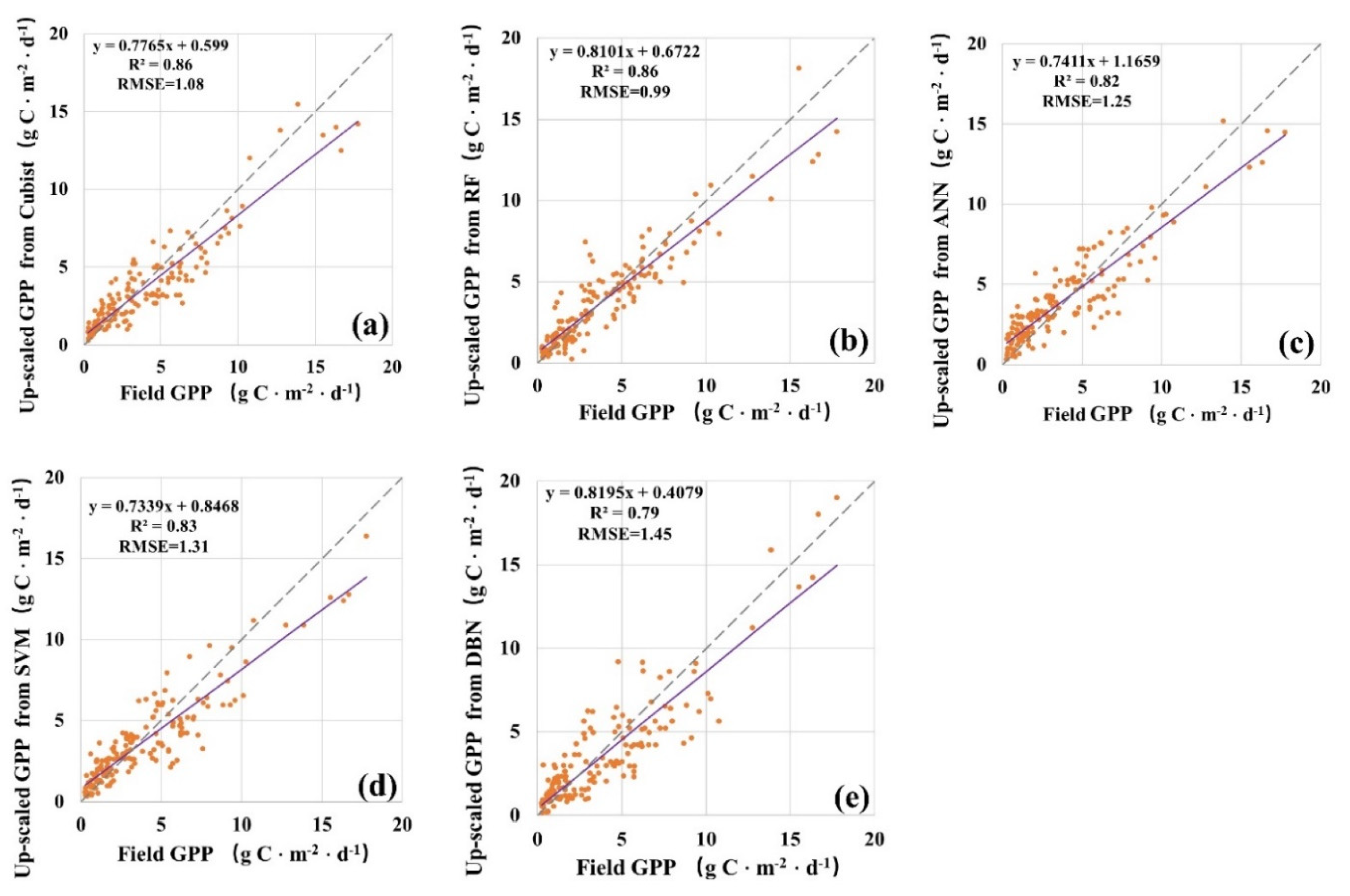
3.1.1. Comparison of Up-Scaled GPP with GPP at Flux Tower Sites

The up-scaled GPP with a spatial resolution of 1 km in 2014 are shown in Figure 3. We found that the spatial distribution of up-scaled GPP, using five machine learning methods, were generally consistent. However, GPP using SVM were higher than those using other models (Cubist, RF, ANN and DBN) in upstream areas. While the opposite situation occurs in the downstream areas; GPP from SVM were lower than those using other models (Cubist, RF, ANN and DBN). In the middle stream, GPP from RF and DBN were higher than those using other models (Cubist, SVM and ANN).
In general, a good linear relationship exists between up-scaled GPP and GPP at flux tower sites, as shown in Figure 4. R2 was as high as 0.86 and RMSE was only 0.99 g C m−2 d−1 of the up-scaled GPP using RF, which demonstrates that up-scaled GPP could obtain the highest accuracy using RF. Followed by up-scaled GPP using Cubist, R2 was 0.86 and RMSE was 1.08 g C m−2 d−1. Up-scaled GPP using DBN gained the lowest precision, R2 was 0.79 and RMSE was 1.45 g C m−2 d−1. The accuracy of up-scaled GPP using RF were the highest.

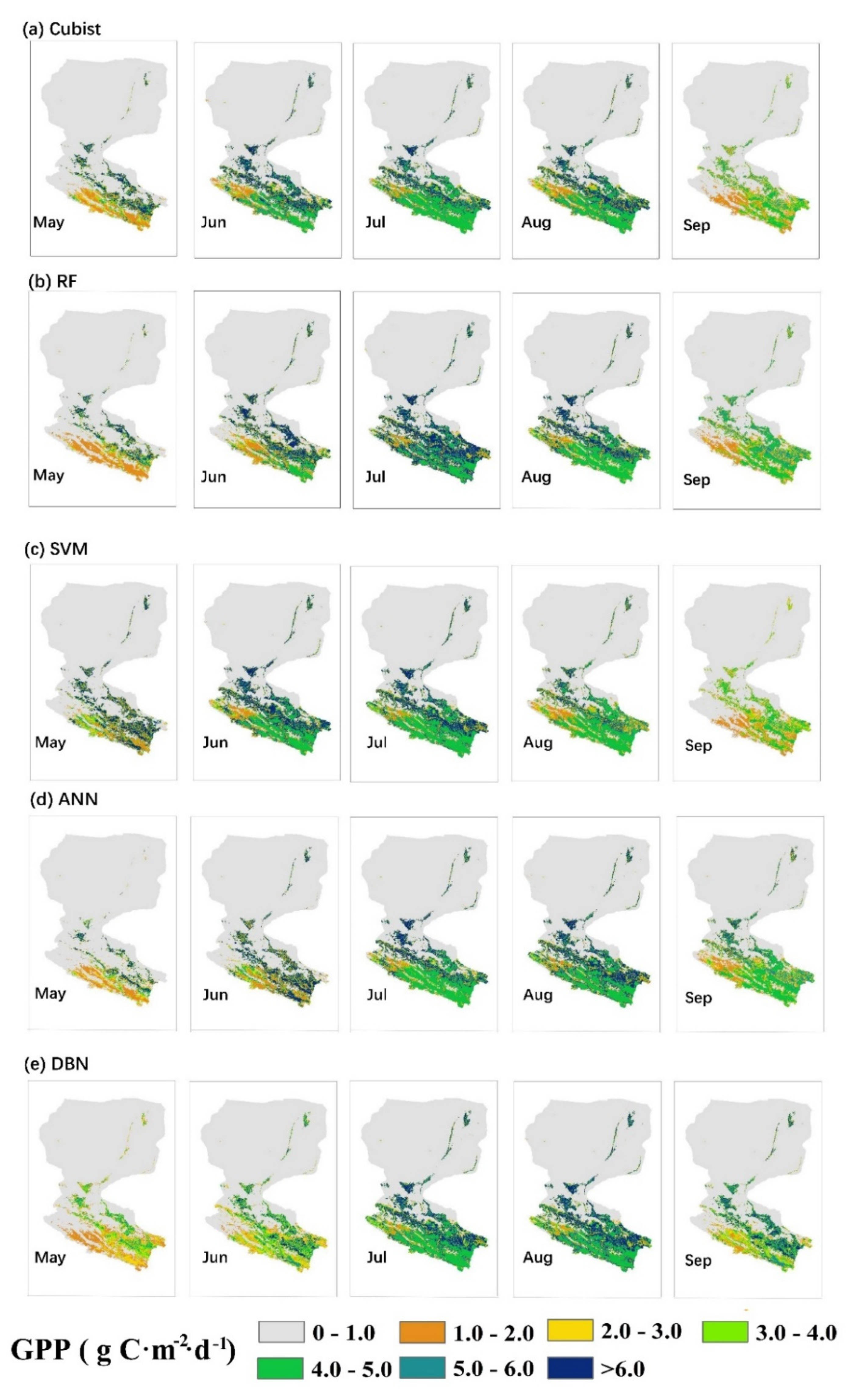
3.1.2. Time Series of the Up-Scaled GPP Using Machine Learning Models

Temporal dynamic patterns of the up-scaled GPP using machine learning methods in nine eddy covariance systems are shown in Figure 5. In general, up-scaled GPP using five machine learning methods could reflect the time series of GPP at flux tower sites. The time series of up-scaled GPP agreed well with GPP in Daman (cropland), Shidi (wetland) and Arou (grassland). Up-scaled GPP using RF agree well with GPP in Sidaoqiao (shrub land), Huyanglin (DBF), Arou (grassland) and Dashalong (grassland). In Daman (cropland, mainly maize), RMSE was the least using SVM. In Huazhaizi (bare land) and Bajitan (bare land), RMSE were the highest using ANN. On the whole, up-scaled GPP using Cubist and DBN could most accurately reflect the temporal dynamic patterns of GPP at flux tower sites.

3.2. Validation of Up-Scaled GPP at Footprint Scale

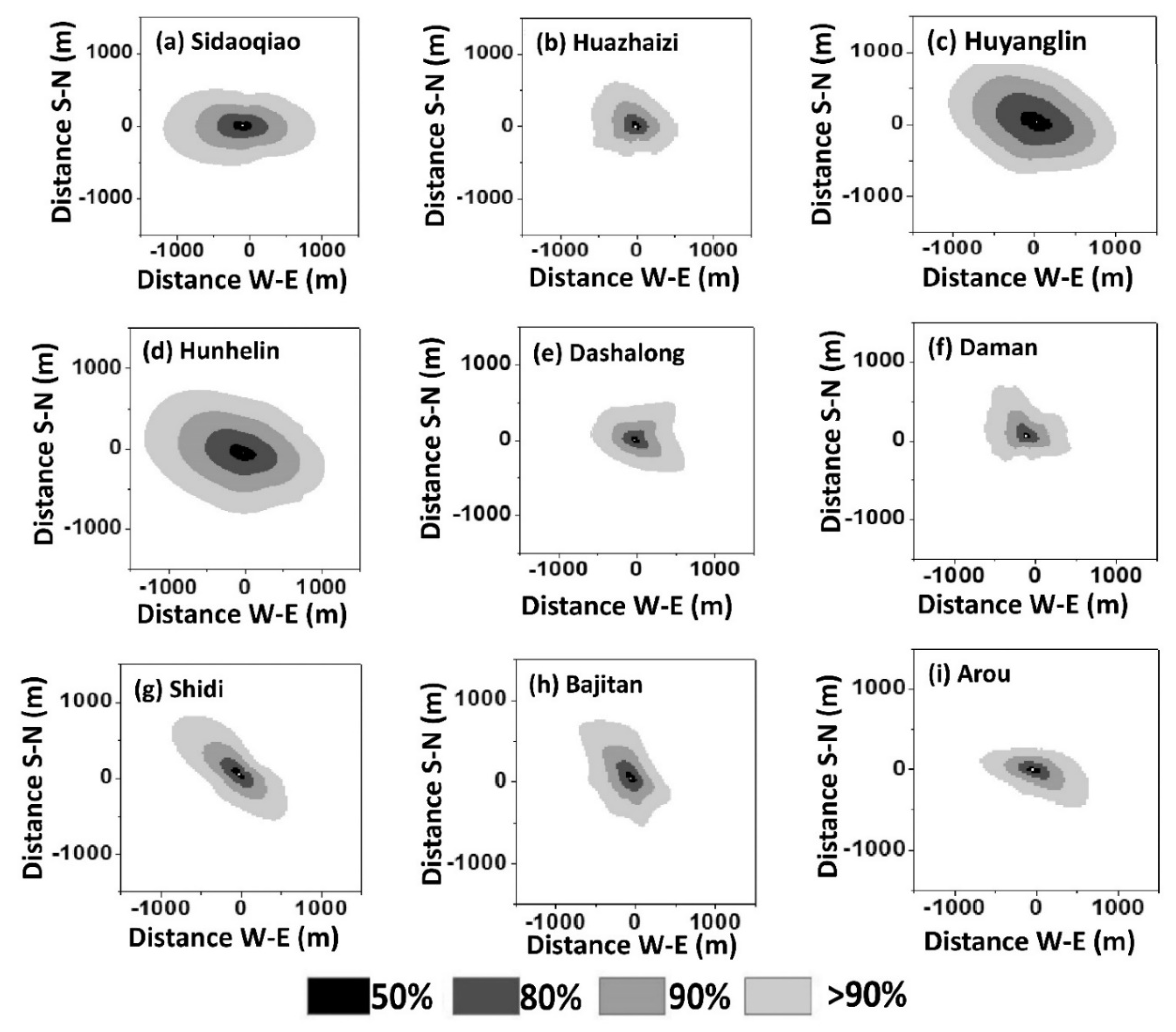
3.2.1. Footprint of GPP at Flux Tower Sites

The climate footprints of GPP at flux tower sites in the study area are shown in Figure 6. In the upstream area, we found that the footprint distances in the northwest to southeast directions were about 500 m to 1000 m, while the footprint distance was less than 300 m in the other directions at Arou (grassland). Moreover, the GPP footprint distances were less than 500 m, and were mainly distributed in the northwest, southeast, and southwest at Dashalong (grassland). In the middle stream area, the prevailing winds were southwest in Huazhaizi (bare land), southeast and northwest in Shidi (wetland), west and northwest in Daman (cropland), and north and southwest in Bajitan (bareland). The GPP footprint distances ranged from 500 m to 1000 m. In the downstream area, the GPP footprint distances at Huyanglin (DBF) and Hunhelin (MF) ranged from 1200 m to 1500 m, and the GPP footprints ranged from 800 m to 1200 m. As the prevailing wind directions were west and northwest in the downstream, the footprints were also mainly distributed in those directions.
The height of the eddy covariance systems was one of the main influence factors of the GPP footprint [7,9]. Heights of the eddy covariance systems were the highest in Huyanglin (22.00 m) and Hunhelin (22.00 m), in which the footprint distances were more than 800 m. While the height of the eddy covariance systems in Huazhaizi (2.85 m) and Arou (3.50 m) were the lowest, the footprint distances were less than 200 m. We analyzed the changes in the GPP footprint distance at flux tower sites, with the changes in measurement height (Figure 7). The footprint distance would decrease by about 43.9–65.2% when the height of the eddy covariance systems decreased by 50%. While the footprint distance would increase by about 56.5–74.9% with the 50% increase in the height of the eddy covariance systems.

3.2.2. Validation of Up-Scaled GPP at Footprint Scale

The weighted GPP in the footprints were obtained according to the contribution rate, and were compared with the up-scaled GPP using machine learning methods (Figure 8). We found that a good linear relationship existed between the up-scaled GPP and GPP in the footprint at flux tower sites (R2 ranged from 0.80 to 0.88, and RMSE ranged from 0.89 g C m−2 d−1 to 1.24 g C m−2 d−1). Compared with the validation against filed GPP directly, we found that the accuracy was higher when validating the up-scaled GPP at the footprint scale. R2 could be as high as 0.88 and RMSE was only 0.89 g C m−2 d−1 of the up-scaled GPP using RF, which also demonstrates that up-scaled GPP could obtain the highest accuracy using RF.

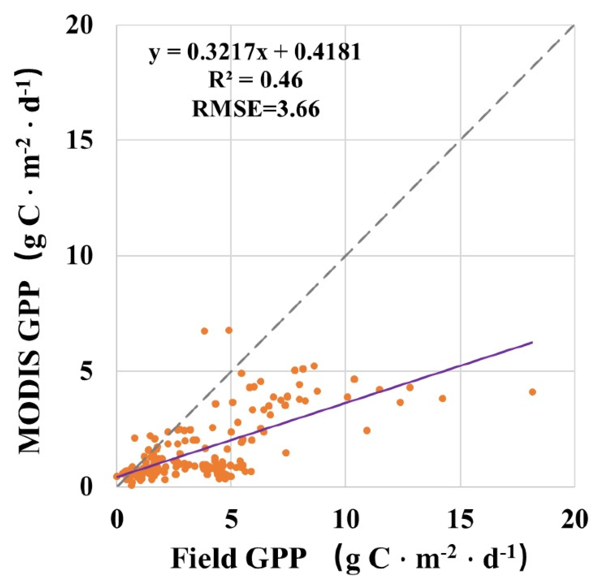
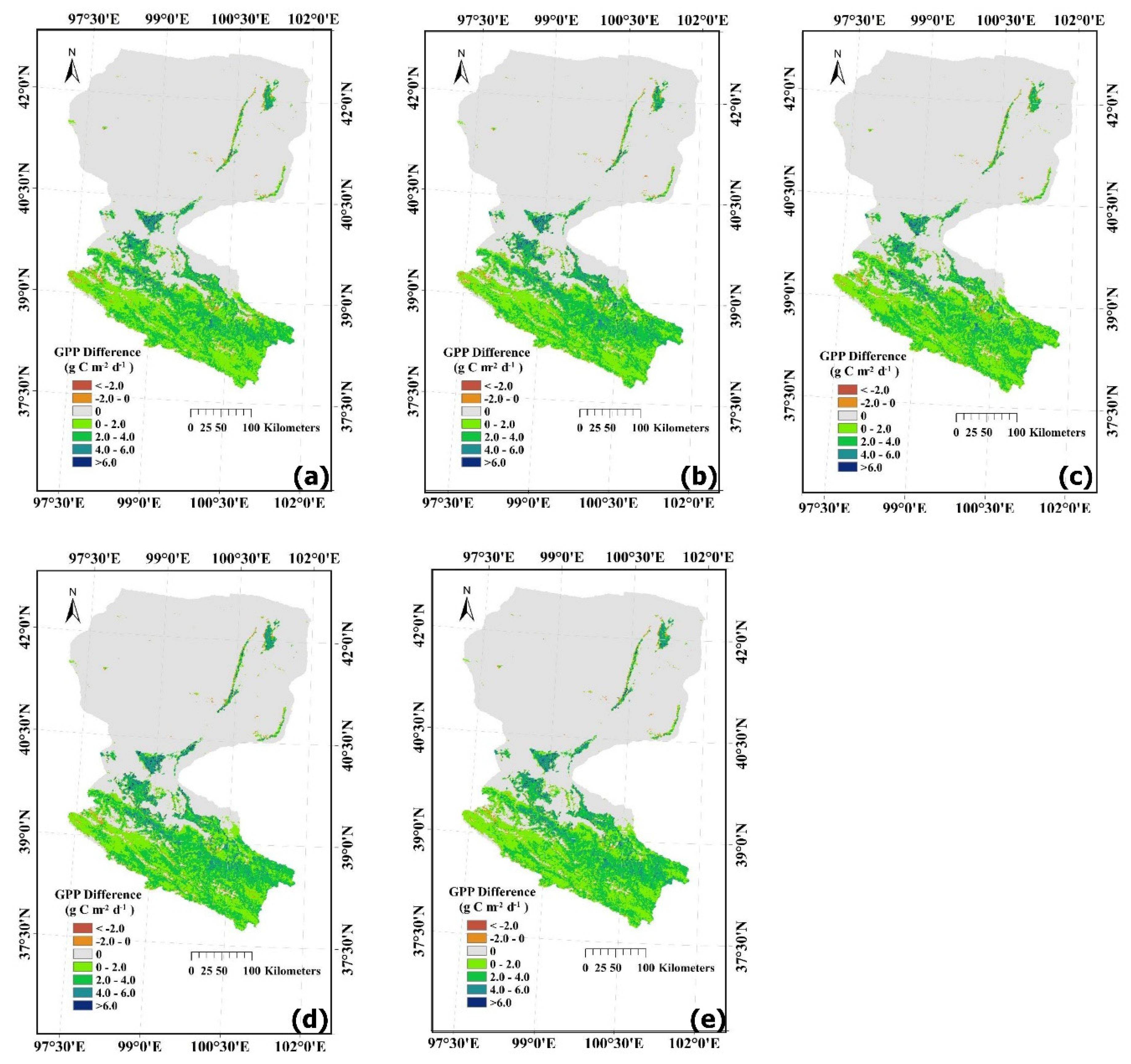
3.3. Cross Comparison with MODIS Products

We compared the averaged up-scaled GPP in the growing season (from May to September 2014) with corresponding MODIS GPP products, pixel by pixel, as shown in Figure 9. In general, a good linear relationship existed between the up-scaled GPP and MODIS GPP (R2 ranged from 0.81 to 0.84, and RMSE ranged from 0.68 g C m−2 d−1 to 0.89 g C m−2 d−1). The up-scaled GPP using RF had the strongest relationships with MODIS GPP (R2 was 0.83 and RMSE was 0.68 g C m−2 d−1). However, we could also found that most the plots in Figure 9 were distributed above the 1:1 line, which indicated that up-scaled GPP using machine learning methods were higher than MODIS GPP products in most cases. To illustrate this, we compared the MODIS GPP with GPP at flux tower sites, as shown in Figure 10. Although a good linear relationship existed between the MODIS GPP and GPP at flux tower sites, most the plots were distributed under the 1:1 line, which demonstrated that the MODIS GPP products were underestimated in the study area, and lead to a high error (RMSE = 3.66 g C m−2 d−1). Previous studies [30] have also shown that in the Heihe River Basin, MODIS GPP products were underestimated. Therefore, in this paper, up-scaled GPP using machine learning methods were higher than MODIS GPP in most cases.
Figure 11 demonstrated the difference of up-scaled GPP and MODIS GPP. We found that spatial distribution of up-scaled GPP was consistent with MODIS GPP. The difference of up-scaled GPP with MODIS GPP ranged from 2.00 g C m−2 d−1 to 4.00 g C m−2 d−1 in most of the upstream study area. We also studied the Pearson coefficients between the 8-day up-scaled GPP and 8-day MODIS GPP products from May to September in 2014 (Figure 12). The absolute values of Pearson coefficients were higher than 0.60 in most of the upstream study area.

4. Discussion

4.1. Sensitivity of the Input Data to the Accuracy of Up-Scaled GPP

The uncertainty of the input datasets would have some influence on the accuracy of the up-scaling process. To study how the uncertainty in the output of the up-scaled GPP from machine learning methods can be apportioned to different sources of uncertainty in the inputs data (NDVI, FVC, SWR, RH, Ta), global sensitivity analysis was carried out by using an extended Fourier amplitude sensitivity test (EFAST) [75,76] in this paper. From Table 2, we found that NDVI was the most sensitive variable to the up-scaled GPP, using the five machine learning methods; it was followed by FVC and SWR. RH had the least sensitivity to the up-scaled results. Local sensitivity analysis of the input data to the up-scaled GPP was shown in Table 3. A 0.60–0.86% change would happen in the up-scaled GPP when RH increased by 10% or decreased by 10%, and a 5.77–7.35% change would happen when RH increased by 50% or decreased by 50%. More than 5% change would happen with the corresponding change of 10% in NDVI, SWR and FVC, and about 16.21–36.81% change would happen with the corresponding change of 50% in NDVI, SWR and FVC. From Table 2 and Table 3, we found that up-scaled GPP was sensitive to NDVI and FVC, which were considered to be the indicators to describe the vegetation phenology, and to monitor the terrestrial photosynthetic vegetation activity. SWR had an impact on the photosynthetic intensity; therefore, it was well related to the temporal changes in GPP. While RH and Ta were not sensitive to the changes in GPP compared to NDVI, FVC and SWR.

4.2. Uncertainty Analysis

In the process of up-scaling GPP and assessing the accuracy of the results, the uncertainty of the observed data and the reference data would have some influence on up-scaling and validating the results. Firstly, the ways to derive GPP from the eddy covariance systems would bring some uncertainties in the up-scaling process. The method to process the missing carbon flux data, such as the look-up table and ANN, would induce some errors when interpolating the eddy covariance data. Second, the footprint of field observation data was related with the heights of the eddy covariance instruments, air conditions, and spatial heterogeneity. The errors of calculating the footprint of GPP at the flux sites would certainly bring some uncertainty in validating the up-scaled results. Third, the errors of the input data (NDVI, FVC, SWR, RH, Ta) used in the machine learning models to up-scaled GPP would also have some influence on the precision of the results. The high accuracy of the machine learning methods relied on the high quality of the training data. Although MODIS LSR products, and land-cover products and meteorological datasets have high accuracy, the errors of the MODIS LSR products, land-cover products and meteorological datasets would have some impact on the accuracy of the training data, and also have some influence on the up-scaling GPP using machine learning models.

4.3. Limitations and Future Work

The bias of the training datasets to train the machine learning methods may have introduced some errors into the up-scaling of GPP. In this paper, NDVI, FVC, SWR, RH and Ta were used to train the machine learning method. In the future, some other variables, such as soil moisture, may also be taken into account in the model training. Moreover, we may carry out some research about the error transfers in GPP up-scaling when using the machine learning models.
The errors induced by scale transformation of the input data would bring some uncertainty to the up-scaled results. Interpolation of the meteorological data, aggregation of the land-cover data, and the method to match the field observation data and satellite data would cause some errors in the up-scaling of GPP. Improving the method to match the scales of the training data in the up-scaling of GPP, would be another way to improve the accuracy of the up-scaling results.
Moreover, it is still challenging to assess the performance of the scale transform models. In this paper, up-scaled GPP were validated at the field scale, footprint scale and regional scale. Some cross validation methods would also be adopted in the future to analyze the effects of the up-scaling models.

5. Conclusions

Up-scaling methods in remote sensing provide a new observational approach to extend the scale of GPP estimates. In this paper, GPP from field eddy covariance systems were up-scaled to the regional scale using five machine learning methods (Cubist, RF, SVM, ANN, DBN). Then, footprints of the GPP at flux tower sites were obtained by using an FSAM model. At last, the up-scaled GPP were validated at the field scale, footprint scale and regional scale. The results of this paper demonstrated the applicability and reliability of up-scaling GPP at flux tower sites, with machine learning methods, and up-scaled GPP using RF could obtain the highest accuracy.
Generally, the spatial distributions of up-scaled GPP using five machine learning methods were consistent. Direct validation with GPP at flux tower sites demonstrated that, although up-scaled GPP using machine learning methods (Cubist, RF, SVM, ANN, DBN) could obtain a high accuracy (R2 ranged from 0.79 to 0.86, and RMSE ranged from 0.99 g C m−2 d−1 to 1.45 g C m−2 d−1), up-scaled GPP using RF obtained the highest accuracy (R2 = 0.86, RMSE = 0.99 g C m−2 d−1). Second, compared with validating with GPP at flux tower sites data, better linear relationships were obtained when validating the up-scaled GPP at the footprint scale (R2 ranged from 0.80 to 0.88, and RMSE ranged from 0.89 g C m−2 d−1 to 1.24 g C m−2 d−1). Moreover, the precision of up-scaled GPP using RF was the highest (R2 = 0.88, RMSE = 0.89 g C m−2 d−1). Third, cross comparison with MODIS GPP products demonstrated that a good linear relationship existed between up-scaled GPP and MODIS GPP (R2 ranged from 0.81 to 0.84, and RMSE ranged from 0.68 g C m−2 d−1 to 0.89 g C m−2 d−1). However, up-scaled GPP from machine learning methods were higher than MODIS GPP in most areas.

Author Contributions

For data curation, Q.Z.; writing—original draft preparation, T.Y.; writing—review and editing, R.S.; visualization, T.Y. and Q.Z.; funding acquisition, R.S. All authors have read and agreed to the published version of the manuscript.

Funding

This research was funded by the National Key R&D Program of China (2016YFB0501502, 2017YFA0603002) and the National Natural Science Foundation of China (41531174), and the Fundamental Research Funds of CAF (CAFYBB2021SY009).

Data Availability Statement

MODIS products data used in this study are available at https://modis.gsfc.nasa.gov/data/ (accessed on 20 May 2021), https://earthexplorer.usgs.gov/ (accessed on 20 May 2021). Meteorological data used in this study are available at www.heihedata.org/data (accessed on 20 May 2021).

Acknowledgments

Thanks for the reviewers’ insightful suggestions and comments to revise this paper.

Conflicts of Interest

The authors declare no conflict of interest.

References

  1. Beer, C.; Reichstein, M.; Tomelleri, E.; Ciais, P.; Jung, M.; Carvalhais, N.; Rödenbeck, C.; Arain, M.A.; Baldocchi, D.; Bonan, G.B.; et al. Terrestrial gross carbon dioxide uptake: Global distribution and covariation with climate. Science 2010, 329, 834–838. [Google Scholar] [CrossRef] [Green Version]
  2. Running, S.W. A measurable planetary boundary for the biosphere. Science 2012, 337, 1458–1459. [Google Scholar] [CrossRef] [Green Version]
  3. Schimel, D.; Stephens, B.B.; Fisher, J.B. Effect of increasing CO2 on the terrestrial carbon cycle. Proc. Natl. Acad. Sci. USA 2015, 112, 436–441. [Google Scholar] [CrossRef] [Green Version]
  4. Yu, T.; Sun, R.; Xiao, Z.; Zhang, Q.; Liu, G.; Cui, T.; Wang, J. Estimation of global vegetation productivity from global land surface satellite data. Remote Sens. 2018, 10, 327. [Google Scholar] [CrossRef] [Green Version]
  5. Chen, J.M.; Mo, G.; Pisek, J.; Liu, J.; Deng, F.; Ishizawa, M.; Chan, D. Effects of foliage clumping on the estimation of global terrestrial gross primary productivity. Glob. Biogeochem. Cycles 2012, 26, GB1019. [Google Scholar] [CrossRef]
  6. Marceau, D.J.; Hay, G.J. Remote sensing contributions to the scale issue. Can. J. Remote Sens. 1999, 25, 357–366. [Google Scholar] [CrossRef]
  7. Schmid, H.P. Footprint modeling for vegetation atmosphere exchange studies: A review and perspective. Agric. For. Meteorol. 2002, 113, 159–183. [Google Scholar] [CrossRef]
  8. Running, S.W.; Thornton, P.E.; Nemani, R.; Glassy, J.M. Global Terrestrial Gross and Net Primary Productivity from the Earth Observing System; Springer: New York, NY, USA, 2000; pp. 44–57. [Google Scholar]
  9. Yu, T.; Sun, R.; Xiao, Z.; Zhang, Q.; Wang, J.; Liu, G. Generation of high resolution vegetation productivity from a downscaling method. Remote Sens. 2018, 10, 1748. [Google Scholar] [CrossRef] [Green Version]
  10. Badgley, G.; Anderegg, L.D.; Berry, J.A.; Field, C.B. Terrestrial gross primary production: Using NIRV to scale from site to globe. Glob. Chang. Biol. 2019, 25, 3731–3740. [Google Scholar] [CrossRef]
  11. Zhang, L.; Wylie, B.; Loveland, T.; Fosnight, E.; Tieszen, L.L.; Gilmanov, T. Evaluation and comparison of gross primary production estimates for the Northern Great Plains grasslands. Remote Sens. Environ. 2007, 106, 173–189. [Google Scholar] [CrossRef] [Green Version]
  12. Anav, A.; Friedlingstein, P.; Beer, C.; Ciais, P.; Harper, A.; Jones, C.; Murray-Tortarolo, G.; Papale, D.; Parazoo, N.C.; Peylin, P.; et al. Spatiotemporal patterns of terrestrial gross primary production: A review. Rev. Geophy. 2015, 53, 785–818. [Google Scholar] [CrossRef] [Green Version]
  13. Mora, B.; Wulder, M.A.; White, J.C. Segment-constrained regression tree estimation of forest stand height from very high spatial resolution panchromatic imagery over a boreal environment. Remote Sens. Environ. 2010, 114, 2474–2484. [Google Scholar] [CrossRef]
  14. Rigge, M.; Wylie, B.; Zhang, L.; Boyte, S.P. Influence of management and precipitation on carbon fluxes in Great Plains grasslands. Ecol. Indic. 2013, 34, 590–599. [Google Scholar] [CrossRef] [Green Version]
  15. Jung, M.; Verstraete, M.; Gobron, N.; Reichstein, M.; Papale, D.; Bondeau, A.; Robustelli, M.; Pinty, B. Diagnostic assessment of European gross primary production. Glob. Chang. Biol. 2008, 14, 2349–2364. [Google Scholar] [CrossRef]
  16. Jung, M.; Reichstein, M.; Margolis, H.A.; Cescatti, A.; Richardson, A.D.; Arain, M.A.; Arneth, A.; Bernhofer, C.; Bonal, D.; Chen, J.; et al. Global patterns of land-atmosphere fluxes of carbon dioxide, latent heat, and sensible heat derived from eddy covariance, satellite, and meteorological observations. J. Geophys. Res. Biogeosci. 2011, 116, G00J07. [Google Scholar] [CrossRef] [Green Version]
  17. Virkkala, A.M.; Aalto, J.; Rogers, B.M.; Tagesson, T.; Treat, C.C.; Natali, S.M.; Watts, J.D.; Potter, S.; Lehtonen, A.; Mauritz, M.; et al. Statistical upscaling of ecosystem CO2 fluxes across the terrestrial tundra and boreal domain: Regional patterns and uncertainties. Glob. Chang. Boil. 2021, 15659. [Google Scholar] [CrossRef] [PubMed]
  18. Gu, Y.; Wylie, B.K.; Bliss, N.B. Mapping grassland productivity with 250-m eMODIS NDVI and SSURGO over the Greater Platte River Basin, USA. Ecol. Indic. 2013, 24, 31–36. [Google Scholar] [CrossRef]
  19. Gilmanov, T.G.; Tieszen, L.L.; Wylie, B.K.; Flanagan, L.B.; Frank, A.B.; Haferkamp, M.R.; Meyers, T.P.; Morgan, J.A. Integration of CO2 flux and remotely-sensed data for primary production and ecosystem respiration analyses in the Northern Great Plains: Potential for quantitative spatial extrapolation. Glob. Ecol. Biogeogr. 2005, 14, 271–292. [Google Scholar] [CrossRef] [Green Version]
  20. Moffat, A.M.; Beckstein, C.; Churkina, G.; Mund, M.; Heimann, M. Characterization of ecosystem responses to climatic controls using artificial neural networks. Glob. Chang. Boil. 2010, 16, 2737–2749. [Google Scholar] [CrossRef]
  21. Fu, D.; Chen, B.; Zhang, H.; Wang, J.; Black, T.A.; Amiro, B.D.; Bohrer, G.; Bolstad, P.; Coulter, R.; Rahman, A.F.; et al. Estimating landscape net ecosystem exchange at high spatial-temporal resolution based on Landsat data, an improved upscaling model framework, and eddy covariance flux measurements. Remote Sens. Environ. 2014, 141, 90–104. [Google Scholar] [CrossRef]
  22. Papale, D.; Valentini, R. A new assessment of European forests carbon exchanges by eddy fluxes and artificial neural network spatialization. Glob. Chang. Biol. 2003, 9, 525–535. [Google Scholar] [CrossRef]
  23. Tramontana, G.; Ichii, K.; Camps-Valls, G.; Tomelleri, E.; Papale, D. Uncertainty analysis of gross primary production upscaling using Random Forests, remote sensing and eddy covariance data. Remote Sens. Environ. 2015, 168, 360–373. [Google Scholar] [CrossRef]
  24. Huang, Y.; Nicholson, D.; Huang, B.; Cassar, N. Global Estimates of marine gross primary production based on machine learning upscaling of field observations. Glob. Biogeochem. Cycles 2021, 35, e2020GB006718. [Google Scholar] [CrossRef]
  25. Zeng, J.; Matsunaga, T.; Tan, Z.-H.; Saigusa, N.; Shirai, T.; Tang, Y.; Peng, S.; Fukuda, Y. Global terrestrial carbon fluxes of 1999–2019 estimated by upscaling eddy covariance data with a random forest. Sci. Data 2020, 7, 313. [Google Scholar] [CrossRef]
  26. Yang, F.; Ichii, K.; White, M.A.; Hashimoto, H.; Michaelis, A.R.; Votava, P.; Zhu, A.; Huete, A.; Running, S.W.; Nemani, R.R. Developing a continental-scale measure of gross primary production by combining MODIS and AmeriFlux data through Support Vector Machine approach. Remote Sens. Environ. 2007, 110, 109–122. [Google Scholar] [CrossRef]
  27. Desai, A.R. Climatic and phenological controls on coherent regional interannual variability of carbon dioxide flux in a heterogeneous landscape. J. Geophys. Res. 2010, 115, G00J02. [Google Scholar] [CrossRef] [Green Version]
  28. Xiao, J.; Davis, K.J.; Urban, N.M.; Keller, K.; Saliendra, N.Z. Upscaling carbon fluxes from towers to the regional scale: Influence of parameter variability and land cover representation on regional flux estimates. J. Geophys. Res. Biogeosci. 2011, 116, G00J06. [Google Scholar] [CrossRef] [Green Version]
  29. Chen, B.; Ge, Q.; Fu, D.; Yu, G.; Sun, X.; Wang, S.; Wang, H. A data-model fusion approach for upscaling gross ecosystem productivity to the landscape scale based on remote sensing and flux footprint modelling. Biogeosciences 2010, 7, 2943–2958. [Google Scholar] [CrossRef] [Green Version]
  30. Dold, C.; Hatfield, J.L.; Prueger, J.H.; Moorman, T.B.; Sauer, T.J.; Cosh, M.H.; Drewry, D.T.; Wacha, K.M. Upscaling gross primary production in corn-soybean rotation systems in the midwest. Remote Sens. 2019, 11, 1688. [Google Scholar] [CrossRef] [Green Version]
  31. Junttila, S.; Kelly, J.; Kljun, N.; Aurela, M.; Klemedtsson, L.; Lohila, A.; Nilsson, M.B.; Rinne, J.; Tuittila, E.; Vestin, P.; et al. Upscaling northern peatland CO2 fluxes using satellite remote sensing data. Remote Sens. 2021, 13, 818. [Google Scholar] [CrossRef]
  32. Wang, X.; Ma, M.; Li, X.; Song, Y.; Tan, J.; Huang, G.; Zhang, Z.; Zhao, T.; Feng, J.; Ma, Z.; et al. Validation of MODIS-GPP product at 10 flux sites in northern China. Int. J. Remote Sens. 2013, 34, 587–599. [Google Scholar] [CrossRef]
  33. Law, B.; Falge, E.; Gu, L.; Baldocchi, D.; Bakwin, P.; Berbigier, P.; Davis, K.; Dolman, A.; Falk, M.; Fuentes, J. Environmental controls over carbon dioxide and water vapor exchange of terrestrial vegetation. Agric. For. Meteorol. 2002, 113, 97–120. [Google Scholar] [CrossRef] [Green Version]
  34. Chasmer, L.; Kljun, N.; Hopkinson, C.; Brown, S.; Milne, T.; Giroux, K.; Barr, A.; Devito, K.; Creed, I.; Petrone, R. Characterizing vegetation structural and topographic characteristics sampled by eddy covariance within two mature aspen stands using lidar and a flux footprint model: Scaling to MODIS. J. Geophys. Res. Biogeosci. 2011, 116, G02026. [Google Scholar] [CrossRef] [Green Version]
  35. Baret, F.; Morissette, J.T.; Fernandes, R.A.; Champeaux, J.L.; Myneni, R.B.; Chen, J.; Plummer, S.; Weiss, M.; Bacour, C.; Garrigues, S.; et al. Evaluation of the representativeness of networks of sites for the global validation and intercomparison of land biophysical products: Proposition of the CEOS-BELMANIP. IEEE Trans. Geosci. Remote Sens. 2006, 44, 1794–1803. [Google Scholar] [CrossRef]
  36. Campbell, J.; Burrows, S.; Gower, S.; Cohen, W. Bigfoot Field Manual; Technical Report, DE2001-13418; NASA STI: Hampton, VA, USA, 1999.
  37. Cohen, W.B.; Justice, C.O. Validating MODIS terrestrial ecology products: Linking in situ and satellite measurements. Remote Sens. Environ. 1999, 70, 1–3. [Google Scholar] [CrossRef]
  38. Wang, P.; Sun, R.; Hu, J.; Zhu, Q.; Zhou, Y.; Li, L.; Chen, J.M. Measurements and simulation of forest leaf area index and net primary productivity in Northern China. J. Environ. Manag. 2007, 85, 607–615. [Google Scholar] [CrossRef]
  39. Mueller, B.; Seneviratne, S.I.; Jimenez, C.; Corti, T.; Hirschi, M.; Balsamo, G.; Ciais, P.; Dirmeyer, P.; Fisher, J.; Guo, Z.; et al. Evaluation of global observations-based evapotranspiration datasets and IPCC AR4 simulations. Geophys. Res. Lett. 2011, 38, 422–433. [Google Scholar] [CrossRef] [Green Version]
  40. Cui, T.; Wang, Y.; Sun, R.; Qiao, C.; Fan, W.; Jiang, G.; Hao, L.; Zhang, L. Estimating vegetation primary production in the Heihe River Basin of China with multi-source and multi-scale data. PLoS ONE 2016, 11, e0153971. [Google Scholar] [CrossRef] [Green Version]
  41. Pan, X.; Li, X.; Yang, K.; He, J.; Zhang, Y.; Han, X. Comparison of downscaled precipitation data over a mountainous watershed: A case study in the Heihe River Basin. J. Hydrometeorol. 2014, 15, 1560–1574. [Google Scholar] [CrossRef]
  42. Li, X.; Lu, L.; Cheng, G.; Xiao, H. Quantifying landscape structure of the Heihe River Basin, north-west China using FRAGSTATS. J. Arid Environ. 2001, 48, 521–535. [Google Scholar] [CrossRef]
  43. MODIS Land Surface Reflectance Products. Available online: https://modis.gsfc.nasa.gov/data/dataprod/mod09.php (accessed on 20 May 2021).
  44. Vermote, E. MOD09A1 MODIS Surface Reflectance 8-Day L3 Global 500 m SIN Grid V006, NASA EOSDIS Land Processes DAAC. USGS Report. 2015. Available online: https://lpdaac.usgs.gov/products/mod09a1v006/ (accessed on 20 May 2021).
  45. Gutman, G.; Ignatov, A. The derivation of the green vegetation fraction from NOAA/AVHRR data for use in numerical weather prediction models. Int. J. Remote Sens. 1998, 19, 1533–1543. [Google Scholar] [CrossRef]
  46. Landuse/Landcover data of the Heihe River Basin. Available online: https://westdc.westgis.ac.cn (accessed on 20 May 2021). [CrossRef]
  47. Zhong, B.; Ma, P.; Nie, A.H.; Yang, A.X.; Yao, Y.J.; Lv, W.B.; Zhang, H.; Liu, Q.H. Land cover mapping using time series HJ-1/CCD data. Sci. China Earth Sci. 2014, 57, 1790–1799. [Google Scholar] [CrossRef]
  48. Zhong, B.; Yang, A.; Nie, A.; Yao, Y.; Zhang, H.; Wu, S.; Liu, Q. Finer resolution land-cover mapping using multiple classifiers and multisource remotely sensed data in the heihe river basin. IEEE J. Sel. Top. Appl. Earth Obs. Remote Sens. 2015, 8, 4973–4992. [Google Scholar] [CrossRef]
  49. Li, X.; Liu, S.M.; Xiao, Q.; Ma, M.G.; Jin, R.; Che, T.; Wang, W.Z.; Hu, X.L.; Xu, Z.W.; Wen, J.G.; et al. A multiscale dataset for understanding complex eco-hydrological processes in a heterogeneous oasis system. Sci. Data 2017, 4, 170083. [Google Scholar] [CrossRef] [PubMed] [Green Version]
  50. MODIS GPP/NPP Products. Available online: https://modis.gsfc.nasa.gov/data/dataprod/mod17.php (accessed on 20 May 2021).
  51. Running, S.W.; Zhao, M. User’s Guide Daily GPP and Annual NPP (MOD17A2/A3) Products NASA Earth Observing System MODIS Land Algorithm; The Numerical Terradynamic Simulation Group: Missoula, MT, USA, 2015. [Google Scholar]
  52. The Atmospheric forcing data in the Heihe River Basin. Available online: https://www.heihedata.org/data (accessed on 20 May 2021). [CrossRef]
  53. Pan, X.; Li, X. Validation of WRF model on simulating forcing data for Heihe River Basin. Sci. Cold Arid Reg. 2011, 3, 344–357. [Google Scholar]
  54. Li, X.; Cheng, G.; Liu, S.; Xiao, Q.; Ma, M.; Jin, R.; Che, T.; Liu, Q.; Wang, W.; Qi, Y.; et al. Heihe watershed allied telemetry experimental research (hiwater): Scientific objectives and experimental design. Bull. Am. Meteorol. Soc. 2013, 94, 1145–1160. [Google Scholar] [CrossRef]
  55. Liu, S.M.; Xu, Z.W.; Wang, W.; Jia, Z.Z.; Zhu, M.J.; Bai, J.; Wang, J.M. A comparison of eddy-covariance and large aperture scintillometer measurements with respect to the energy balance closure problem. Hydrol. Earth Syst. Sci. 2011, 15, 1291–1306. [Google Scholar] [CrossRef] [Green Version]
  56. Xu, Z.; Liu, S.; Li, X.; Shi, S.; Wang, J.; Zhu, Z.; Xu, T.; Wang, W.; Ma, M. Intercomparison of surface energy flux measurement systems used during the HiWATER-MUSOEXE. J. Geophys. Res. 2013, 118, 13140–13157. [Google Scholar] [CrossRef]
  57. Papale, D.; Reichstein, M.; Aubinet, M.; Canfora, E.; Bernhofer, C.; Kutsch, W.; Longdoz, B.; Rambal, S.; Valentini, R.; Vesala, T.; et al. Towards a standardized processing of Net Ecosystem Exchange measured with eddy covariance technique: Algorithms and uncertainty estimation. Biogeosciences 2006, 3, 571–583. [Google Scholar] [CrossRef] [Green Version]
  58. Zhu, Z.; Sun, X.; Wen, X.; Zhou, Y.; Tian, J.; Yuan, G. Study on the processing method of nighttime CO2 eddy covariance flux data in ChinaFLUX. Sci. China Ser. D 2006, 49, 36–46. [Google Scholar] [CrossRef]
  59. Zhang, L.; Sun, R.; Xu, Z.; Qiao, C.; Jiang, G. Diurnal and seasonal variations in carbon dioxide exchange in ecosystems in the Zhangye oasis area, Northwest China. PLoS ONE 2015, 10, e0120660. [Google Scholar]
  60. Coops, N.C.; Black, T.A.; Jassal, R.P.S.; Trofymow, J.T.; Morgenstern, K. Comparison of MODIS, eddy covariance determined and physiologically modelled gross primary production (GPP) in a Douglas-fir forest stand. Remote Sens. Environ. 2007, 107, 385–401. [Google Scholar] [CrossRef]
  61. Wang, H.; Saigusa, N.; Yamamoto, S.; Kondo, H.; Hirano, T.; Toriyama, A.; Fujinuma, Y. Net ecosystem CO2 exchange over a larch forest in Hokkaido, Japan. Atmos. Environ. 2004, 38, 7021–7032. [Google Scholar] [CrossRef]
  62. Saigusa, N.; Yamamoto, S.; Murayama, S.; Kondo, H.; Nishimura, N. Gross primary production and net ecosystem exchange of a cool-temperate deciduous forest estimated by the eddy covariance method. Agric. For. Meteorol. 2002, 112, 203–215. [Google Scholar] [CrossRef]
  63. Janssens, I.A.; Lankreijer, H.; Matteucci, G.; Kowalski, A.S.; Buchmann, N.; Epron, D.; Pilegaard, K.; Kutsch, W.; Longdoz, B.; Grünwald, T.; et al. Productivity overshadows temperature in determining soil and ecosystem respiration across European forests. Glob. Chang. Boil. 2001, 7, 269–278. [Google Scholar] [CrossRef]
  64. Schmid, H.P. Source areas for scalars and scalar fluxes. Bound. Lay. Meteorol. 1994, 67, 293–318. [Google Scholar] [CrossRef]
  65. Schmid, H.P.; Lloyd, C.R. Spatial representativeness and the location bias of flux footprints over inhomogeneous areas. Agric. For. Meteorol. 1999, 93, 195–209. [Google Scholar] [CrossRef]
  66. Kljun, N.; Kastner-Klein, P.; Fedorovich, E.; Rotach, M.W. Evaluation of Lagrangian footprint model using data from wind tunnel convective boundary layer. Agric. For. Meteorol. 2004, 127, 189–201. [Google Scholar] [CrossRef]
  67. Kljun, N.; Calanca, P.; Rotach, M.W.; Schmid, H.P. A simple two-dimensional parameterisation for Flux Footprint Prediction (FFP). Geosci. Model. Dev. 2015, 8, 3695–3713. [Google Scholar] [CrossRef] [Green Version]
  68. Xiao, J.; Zhuang, Q.; Baldocchi, D.D.; Law, B.E.; Richardson, A.D.; Chen, J.; Oren, R.; Starr, G.; Noormets, A.; Ma, S.; et al. Estimation of net ecosystem carbon exchange for the conterminous United States by combining MODIS and AmeriFlux data. Agric. For. Meteorol. 2008, 148, 1827–1847. [Google Scholar] [CrossRef] [Green Version]
  69. Wang, J.; Sun, R.; Zhang, H.; Xiao, Z.; Zhu, A.; Wang, M.; Yu, T.; Xiang, K. New global MuSyQ GPP/NPP remote sensing products from 1981 to 2018. IEEE J. Sel. Top. Appl. Earth Obs. Remote Sens. 2021, 14, 5596–5612. [Google Scholar] [CrossRef]
  70. Xiao, J.; Zhuang, Q.; Law, B.E.; Chen, J.; Baldocchi, D.D.; Cook, D.R.; Oren, R.; Richardson, A.D.; Wharton, S.; Ma, S.; et al. A continuous measure of gross primary production for the conterminous United States derived from MODIS and AmeriFlux data. Remote Sens. Environ. 2010, 114, 576–591. [Google Scholar] [CrossRef] [Green Version]
  71. Wang, M.; Sun, R.; Zhu, A.; Xiao, Z. Evaluation and Comparison of Light Use Efficiency and Gross Primary Productivity Using Three Different Approaches. Remote Sens. 2020, 12, 1003. [Google Scholar] [CrossRef] [Green Version]
  72. Wei, S.; Yi, C.; Fang, W.; Hendrey, G. A global study of GPP focusing on light-use efficiency in a random forest regression model. Ecosphere 2017, 8, e01724. [Google Scholar] [CrossRef]
  73. Sun, Z.; Wang, X.; Zhang, X.; Tani, H.; Guo, E.; Yin, S.; Zhang, T. Evaluating and comparing remote sensing terrestrial GPP models for their response to climate variability and CO2 trends. Sci. Total Environ. 2019, 668, 696–713. [Google Scholar] [CrossRef]
  74. Jiang, D.; Liu, P.; Ravyse, I.; Sahli, H.; Verhelst, W. Video realistic mouth animation based on an audio visual DBN model with articulatory features and constrained asynchrony. In Proceedings of the 2009 Fifth International Conference on Image and Graphics, Xi’an, China, 20–23 September 2009; IEEE: Piscataway, NJ, USA, 2009; pp. 658–662. [Google Scholar]
  75. Iooss, B.; Lemaître, P. A review on global sensitivity analysis methods. In Uncertainty Management in Simulation-Optimization of Complex Systems; Springer: Boston, MA, USA, 2015. [Google Scholar]
  76. Saltelli, A.; Tarantola, S.; Chan, K.S. A quantitative model-independent method for global sensitivity analysis of model output. Technometrics 1999, 41, 39–56. [Google Scholar] [CrossRef]
Figure 1. Location and land-cover types of the study area. Bare lands are mainly distributed in the downstream in the northern areas, forests and croplands are mainly distributed in the upstream in southern areas.
Remotesensing 13 02448 g001
Figure 2. Flowchart of up-scaling and validation of GPP. Five machine learning methods were used to up-scale GPP from field to regional scale, then the results were validated at field scale, at footprint scale and at regional scale.
Remotesensing 13 02448 g002
Figure 3. Up-scaled GPP using (a) Cubist, (b) RF, (c) ANN, (d) SVM, (e) DBN from May to September in 2014.
Remotesensing 13 02448 g003
Figure 4. Validation of up-scaled GPP using (a) Cubist, (b) RF, (c) ANN, (d) SVM, (e) DBN against GPP at flux tower sites. These figures demonstrate the relationship between 8-day average GPP at flux tower sites and 8-day average up-scaled GPP from May to September in 2014 using five machine learning methods. The solid line is the fit line between GPP at flux tower sites and up-scaled GPP, and the dashed line is the 1:1 line.
Remotesensing 13 02448 g004
Figure 5. Time series of up-scaled GPP using five machine learning models in (a) Sidaoqiao, (b) Huazhaizi, (c) Huyanglin, (d) Hunhelin, (e) Dashalong, (f) Daman, (g) Shidi, (h) Bajintan, (i) Arou. These figures demonstrate time series of 8-day average GPP at flux tower sites and 8-day average up-scaled GPP from May to September in 2014 using five machine learning methods.
Remotesensing 13 02448 g005
Figure 6. Climate footprint of GPP at flux tower sites in (a) Sidaoqiao, (b) Huazhaizi, (c) Huyanglin, (d) Hunhelin, (e) Dashalong, (f) Daman, (g) Shidi, (h) Bajintan, (i) Arou. The x-coordinate is the distance of footprint at east–west direction, y-coordinate is the distance of footprint at north–south direction. The gray level means cumulative weight the contribution of the footprint.
Remotesensing 13 02448 g006
Figure 7. Changes in climate footprint distance of GPP at flux tower sites with the changes in measurement height. This figure shows the changes in GPP footprint distance when the measurement heights increase 50% or decrease 50%.
Remotesensing 13 02448 g007
Figure 8. Validation of up-scaled GPP using (a) Cubist, (b) RF, (c) ANN, (d) SVM, (e) DBN at footprint scale. These figures demonstrate the relationship between 8-day weighted average GPP at flux tower sites in the footprint and 8-day average up-scaled GPP from May to September in 2014 using five machine learning methods. The solid line is the fit line between GPP at flux tower sites in the footprint and up-scaled GPP, and the dashed line is the 1:1 line. Accuracy of up-scaled GPP using RF were the highest.
Remotesensing 13 02448 g008
Figure 9. Comparison of up-scaled GPP using (a) Cubist, (b) RF, (c) ANN, (d) SVM, (e) DBN with MODIS GPP pixel by pixel. These figures demonstrate the relationship between MODIS GPP (8-day, 1000 m) and 8-day average up-scaled GPP from May to September in 2014 using five machine learning methods. The solid line is the fit line between MODIS GPP and up-scaled GPP, and the dashed line is the 1:1 line. The number of pixels is 23268 (n = 23268). Due to the underestimation of MODIS GPP products, up-scaled GPP using machine learning methods were higher than MODIS GPP products in most cases.
Remotesensing 13 02448 g009
Figure 10. Validation of MODIS GPP against GPP at flux tower sites. MODIS GPP products were underestimated compared with GPP at flux tower sites. The solid line is the fit line between GPP at flux tower sites and MODIS GPP, and the dashed line is the 1:1 line.
Remotesensing 13 02448 g010
Figure 11. Difference in up-scaled GPP using (a) Cubist, (b) RF, (c) ANN, (d) SVM, (e) DBN with MODIS GPP. Up-scaled GPP were higher than MODIS GPP in most areas.
Remotesensing 13 02448 g011
Figure 12. Pearsons of up-scaled GPP using (a) Cubist, (b) RF, (c) ANN, (d) SVM, (e) DBN with MODIS GPP.
Remotesensing 13 02448 g012
Table 1. Information of the carbon flux observation stations. DBF (deciduous broadleaved forest), MF (mixed forest).
NameLongitude (°)Latitude (°)Altitude (m)Height of
Instruments (m)
LocationLand Cover
Arou100.4638.0530333.50UpstreamGrassland
Dashalong98.9438.8437394.50UpstreamGrassland
Bajitan100.3038.9215624.60MidstreamBare land
Daman100.3738.8615564.50MidstreamCropland
Huazhaizi100.3238.7717312.85MidstreamBare land
Shidi100.4538.9814605.20MidstreamWetland
Huyanglin101.1241.9987622.00DownstreamDBF
Hunhelin101.1341.9987422.00DownstreamMF
Didaoqiao101.1442.008738.00DownstreamShrub land
Table 2. Global sensitivity analysis of the input data to the up-scaled GPP. FVC (fractional vegetation cover), SWR (shortwave radiation), Ta (air temperature), RH (relative humidity), NDVI (normalized difference vegetation index), ANN (artificial neural network), RF (random forest), SVM (support vector machine), DBN (deep belief network).
ANN (%)Cubist (%)RF (%)SVM (%)DBN (%)
FVC2221222420
SWR2116222125
Ta1721211822
RH811697
NDVI3231292826
Table 3. Local sensitivity analysis of the input data to the up-scaled GPP. Specifically, we studied the effect of increasing or decreasing variables by 10% and 50%, while holding other variables constant. FVC (fractional vegetation cover), SWR (shortwave radiation), Ta (air temperature), RH (relative humidity), NDVI (normalized difference vegetation index), ANN (artificial neural network), RF (random forest), SVM (support vector machine), DBN (deep belief network).
ANN (%)Cubist (%)RF (%)SVM (%)DBN (%)
FVC ± 10%4.695.035.714.625.82
FVC ± 50%16.8320.6121.9216.2122.23
SWR ± 10%6.778.557.637.238.02
SWR ± 50%18.6936.8122.3420.0830.21
Ta ± 10%2.633.242.983.652.74
Ta ± 50%12.4416.5014.3318.9213.21
RH ± 10%0.690.860.600.720.77
RH ± 50%5.947.355.776.256.94
NDVI ± 10%6.998.347.518.427.02
NDVI ± 50%26.7830.8429.6634.0228.21
Publisher’s Note: MDPI stays neutral with regard to jurisdictional claims in published maps and institutional affiliations.

