Quantitatively Estimating of InSAR Decorrelation Based on Landsat-Derived NDVI

Abstract

As a by-product of Interferometric Synthetic Aperture Radar (SAR, InSAR) technique, interferometric coherence is a measure of the decorrelation noise for InSAR observation, where the lower the coherence value, the more serious the decorrelation noise. In the densely vegetated area, the coherence value could be too low to obtain any valuable signals, leading to the degradation of InSAR performance and the possible waste of expensive SAR data. Normalized Difference Vegetation Index (NDVI) value is a measure of the vegetation coverage and can be estimated from the freely available optical satellite images. In this paper, a multi-stage model is established to quantitatively estimate the decorrelation noise for vegetable areas based on Landsat-derived NDVI prior to the acquisition of SAR data. The modeling process is being investigated with the L-band ALOS-1/PALSAR-1 data and the Landsat-5 optical data acquired in the Meitanba area of Hunan Province, China. Furthermore, the reliability of the established model is verified in the Longhui area, which is situated near the Meitanba area. The results demonstrate that the established model can quantitatively estimate InSAR decorrelation associated with the vegetation coverage.

1. Introduction

Interferometric Synthetic Aperture Radar (InSAR) has proved to be an effective tool for monitoring surface deformation with its advantages of all-weather, all-day, large-scale, and satisfactory precision [1,2,3,4,5]. However, as repeat-pass interferometry, InSAR is very sensitive to vegetation coverage on the ground since the deformation signal is susceptible to the serious decorrelated noise due to vegetation changes during the revisiting period of SAR images [6]. Especially for SAR data with short wavelengths, decorrelated noise can even swamp the deformation signal [7]. As a result, the reliability and accuracy of the InSAR deformation monitoring results are not stable in the vegetable area. It is difficult to accurately judge the monitoring performance of the SAR data used in the area of interest prior to the acquisition of SAR data, which means that there is certain blindness in data selection. This will result in InSAR technology failing to perform its best in subsequent deformation monitoring and interpretation, and even lead to the waste of expensive data resources. In recent years, the rapid development of SAR satellites has provided a wide space for data selection in the monitoring of surface deformation. Different parameters (e.g., polarization modes, incident angles, and spatial resolutions) can be customized according to actual needs. It will become a normal trend to integrate multiple (including multi-temporal, multi-orbit, multi-frequency, and multi-polarization) SAR data for surface deformation monitoring. If the performance of InSAR deformation measurements can be accurately estimated before acquiring SAR data, it can not only help to select the most suitable SAR data configuration, but also provide a way to access the accuracy of SAR data.

As one of the most important indexes for evaluating the performance of InSAR measurement, coherence can be divided into spatial and temporal components [8]. The spatial coherence properties can be calculated by theoretical formulas, but the temporal coherence cannot be directly measured [9]. In general, the temporal coherence can be separated from the total coherence by removing other components based on the composition principle of coherence [10]. Tian et al. [11] proposed a method for temporal decorrelation analysis of echo signals, but the essence of this method is still based on the decomposition of coherence.

Temporal decorrelation is mainly caused by the change of scattering characteristics of ground objects during the satellite revisit period [12,13]. Therefore, in a vegetable area, the decorrelation caused by vegetation change dominates the temporal decorrelation. The most direct way to evaluate the decorrelation noise is to find the relationship between vegetation cover and temporal decorrelation. To date, some preliminary attempts had been made. Coherence has been widely used in land classification, but its relationship with vegetation coverage is rarely quantified [14,15]. It has been confirmed that the performances of the coherences are different for various types of vegetation cover [16,17]. In addition, both the height and density of vegetation are important factors affecting coherence [18]. In general, coherence and vegetation density show a negative correlation, that is, coherence decreases with the increase of vegetation density [19]. Some studies had suggested that there was a certain non-linear relationship between coherence and some vegetation indices, but the reliability of this relationship needs to be verified [20]. Most of these pieces of research focus on the qualitative analysis [21,22], while the quantitative relationship between coherence and vegetation coverage is still unclear.

Normalized Difference Vegetation Index (NDVI) is a widely used measurement of vegetation coverage, which can be derived from freely available optical satellite images (e.g., Landsat images) [23]. It had been proved that coherence is related to NDVI [20,24,25,26]. This provides an opportunity for the quantitative estimation of InSAR decorrelation noise. In this paper, based on the ALOS-1/PALSAR-1 and Landsat5 images acquired in Meitanba area, Hunan Province, China, we found a nonlinear relationship between InSAR coherence and NDVI, and established a multi-stage model to quantitatively estimate decorrelation noise. In addition, the performance of the established model was assessed in Longhui area, Hunan Province, China.

This paper is organized as follows. In the next section, the study area and the processing procedures of Landsat5 and ALOS-1/PALSAR-1 data are described in detail. The proposed method for establishing the model is introduced in Section 3. Section 4 is dedicated to the presentation of the obtained results. Finally, conclusions and further thoughts are addressed.

2. Study Area and Datasets

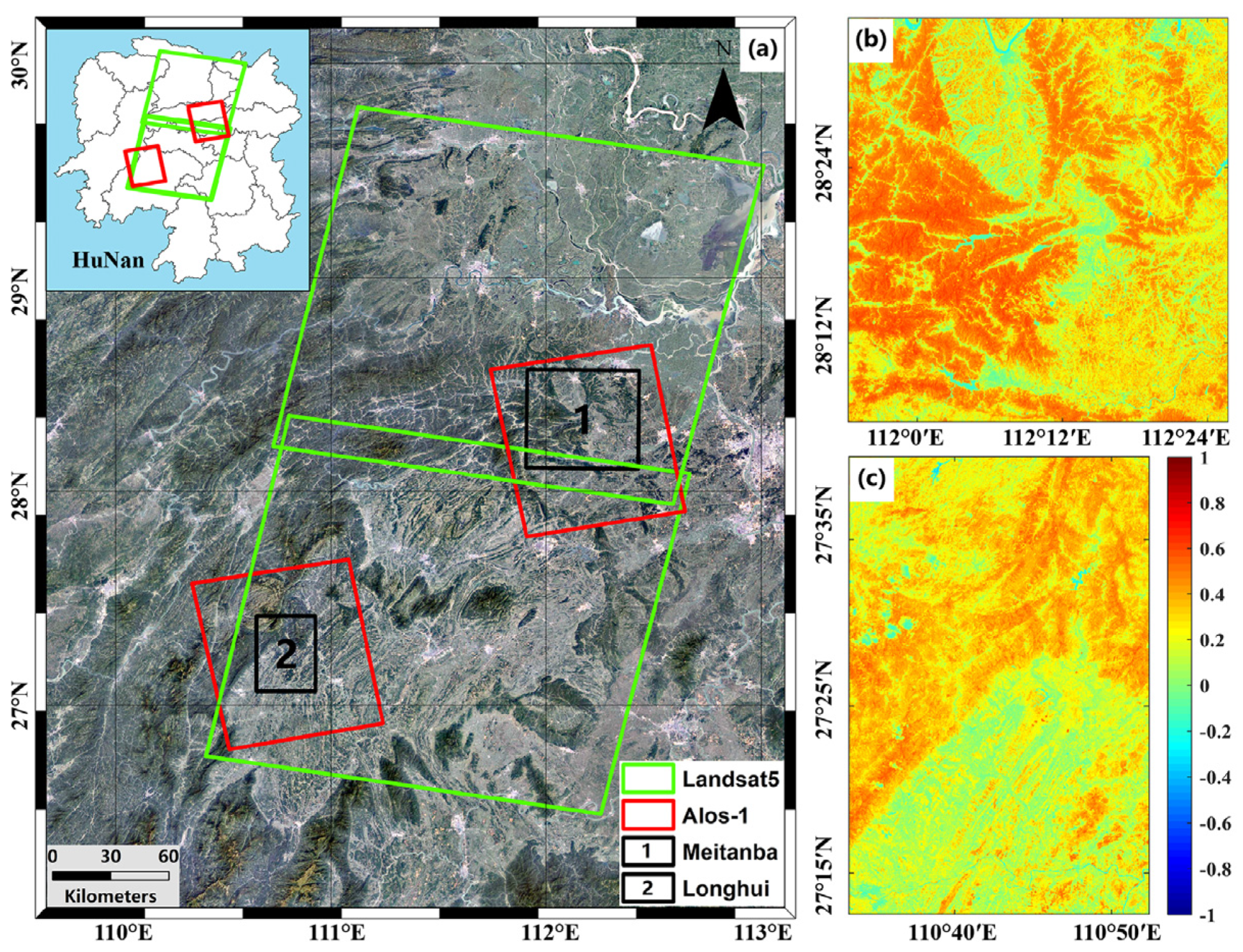
2.1. Study Area

The test site is the Meitanba area located in Hunan Province, China (see Figure 1a). There is abundant vegetation in this area. Since this area is characterized by gentle terrain and the slope angles are basically less than 10°, the influence of spatial decorrelation is small. In addition, we chose Longhui area as the validation area to further verify the reliability of the decorrelation evaluation model. Longhui area is also located at Hunan Province and near the Meitanba area (see Figure 1a), where vegetation is dense and the terrain is complex and diverse. To reduce the influence of topography, the areas with relatively flat terrain are selected.

2.2. Landsat5 Data

In this study, we collected the cloud-free Landsat5 TM images acquired in May 2008, which is used to represent the vegetation coverage in the study area (

Table 1. Landsat5 images used in the study.

Location	Data	Resolution
Meitanba	21 May 2008	30 m
Longhui	21 May 2008

). First, radiation calibration and atmospheric correction were both carried out for the used Landsat5 TM images, which produced the reflectivity values of the red and near-infrared bands. Then, the common areas were extracted by selecting control points for image registration and mosaic clipping. Finally, the NDVI value was derived based on the Landsat5 images by using Equation (1).

$$NDVI=\frac{P_{NIR}-P_{RED}}{P_{NIR}+P_{RED}}$$

(1)

where $P_{NIR}$ and $P_{RED}$ are the reflectance values in near-infrared and red bands, respectively. NDVI is commonly used to monitor vegetation cover and growth, whose range is in [−1,1]. The negative value indicates that the surface coverages are water, ice, or snow, which have very high reflectivity to visible light. Zero indicates bare soil, rock, or buildings. The positive value refers to the presence of vegetation, and the value of NDVI increases with the increase of vegetation coverage. The NDVI results in Meitanba area and Longhui area are shown in Figure 1b,c, respectively.

2.3. ALOS-1/PALSAR-1 Data

Ascending PALSAR-1 images in HH polarization modes acquired by ALOS-1 satellite are employed in the study. The incident angle is 38.74 degrees (

Table 2. ALOS-1/PALSAR-1 images used in the study.

Location	Master Date	Slave Date	Bt	B⊥	Resolution
Meitanba	11 January 2008	26 February 2008	46 day	437 m	30 m
Longhui	16 January 2008	17 April 2008	92 day	752 m

). The SAR interferometric image pairs were processed with two-pass differential interferometry. Multi-look processing was adopted to suppress noises as well as to resample the PALSAR-1 images to the same resolution as the Landsat5 images.

Coherence represents the degree of similarity between two single-look complex images (SLC). It is often used to evaluate the quality of interference fringes, as is the correlation coefficient between two real images. The greater the coherence, the higher the quality of InSAR observation. Coherence measure $\gamma$ is defined as the magnitude of the correlation coefficient between two accurately co-registered complex images $u_1$ and $u_2$ [27]

$$\gamma =\frac{\left|E\left[u_1{u}_2^{\ast }\right]\right|}{\sqrt{E\left[{\left|u_1\right|}^2\right]E\left[{\left|u_2\right|}^2\right]}}$$

(2)

where $E[·]$ indicates the mathematical expectation and the symbol $\ast$ represents complex conjugate. The total coherence is the sum of geometric decorrelation, temporal decorrelation, and thermal decorrelation. Thermal noise is generally ignored, and geometric coherence can be removed according to [9]. In addition, to ensure that the coherence and NDVI images are in the same coordinate system, the Landsat5 and PALSAR-1 images are co-registered based on the 1 arcsecond SRTM DEM.

3. Methodology

In this section, the modeling process is demonstrated in detail by exploiting the Landsat5 and PALSAR-1 images acquired in the Meitanba area. However, it is difficult to build a model directly from the data since gross errors will degrade the correlation between coherence and NDVI. For example, the measurements of NDVI are sensitive to soil moisture and atmosphere [28]. InSAR coherence observations are greatly affected by the window size used in the calculation [8]. As a result, no obvious trend can be obtained between coherence and NDVI when the data are directly used. Therefore, a novel sampling procedure was proposed to eliminate gross errors before building the model.

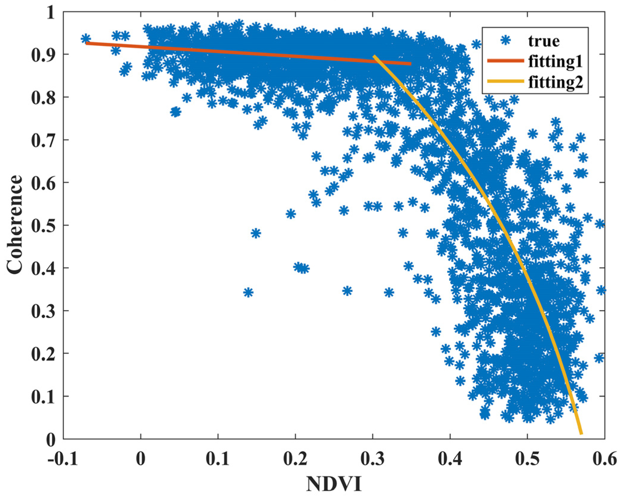
3.1. Sampling Based on Correlation Estimation Model

The proposed sampling procedure is based on a correlation estimating model and includes three steps. First, for the interesting pixel position, two moving windows of the same sizes were opened in the NDVI and coherence images, respectively, which had been co-registered. Second, the correlation coefficient of all the pixels in the two windows was calculated based on the basic idea of the Pearson correlation coefficient [29]. If the correlation coefficients of the two moving windows meet the preset threshold, all the pixels in the two windows are taken as observation samples, otherwise, these pixels are discarded. Third, the previous operations were conducted window-by-window until the entire image was traversed by the moving window. Because the quality of the observed data is affected by many uncertainties, the optimal window size and correlation threshold could be different for the sampling of different data. As for the selection of moving window and correlation threshold, we carried out a large number of experiments with different values and found that a window size of 50 × 50 and a threshold of 0.8 could yield ideal results, which were used to select samples in this study. The correlation coefficient of the two windows is calculated by Equation (3).

$$R=\frac{{{\displaystyle \sum }}_m{{\displaystyle \sum }}_n\left(A_{mn}-\overline{A}\right)\left(B_{mn}-\overline{B}\right)}{\sqrt{\left({{\displaystyle \sum }}_m{{\displaystyle \sum }}_n{\left(A_{mn}-\overline{A}\right)}^2\right)\left({{\displaystyle \sum }}_m{{\displaystyle \sum }}_n{\left(B_{mn}-\overline{B}\right)}^2\right)}}$$

(3)

where$R$ is the correlation coefficient between the two windows,$m$ and$n$ represent the sizes of the window. $\overline{A}$ and $\overline{B}$ represent the average values of all the pixels in two windows, respectively. The schematic diagram of the proposed sampling procedure is shown in Figure 2.

3.2. Effect of Perpendicular-Temporal Baseline Variation

In order to consider the effect of time, the relationship between perpendicular-temporal baselines and coherence is analyzed. Figure 3a shows the coherence variations over temporal and spatial baselines associated with the ALOS-1 interferograms acquired in the Meitanba area. As observed, the effect of temporal baseline on coherence is greater than that of spatial baseline. This is because the topography of the study area is relatively flat and the effect of spatial decorrelation is small in the L-band observation. In addition, the spatial coherence has been removed based on the theoretical formula [9] when establishing the model. Figure 3b shows the coherence decreases exponentially with temporal baselines, proving that coherence is highly dependent on temporal baselines. Therefore, it is reasonable to add an exponential decay factor to the model. The orange curve represents the coherence as a function of temporal baselines, fitted by the iterative least squares method. The coefficients $a$ and $\tau$ were then obtained as 0.87 and 172 days, respectively, with 95% confidence interval.

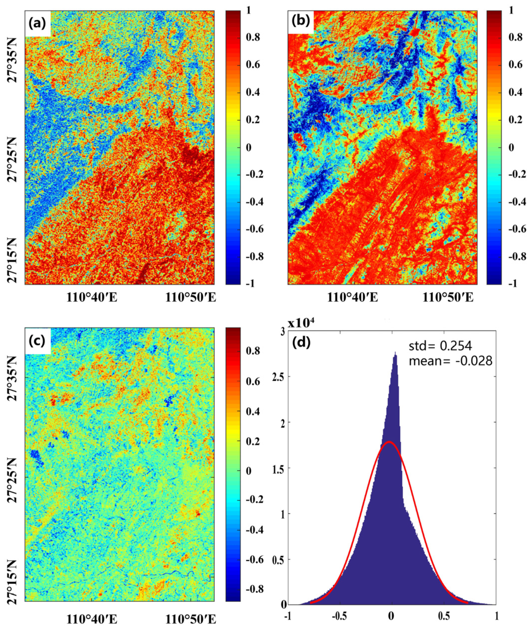
3.3. Establishment of Decorrelation Noise Model

The data selected by the proposed sampling procedure were analyzed in order to investigate the relationship between the Landsat5/NDVI and PALSAR-1/coherence in Meitanba area. As shown in Figure 4, it is obvious that there is a strong correlation between the NDVI and the coherence of the study area. In the areas with high vegetation coverage, the coherence of the SAR image is low. On the contrary, the coherence of the SAR image is high in the areas with low vegetation coverage. This is consistent with the actual situation. When the NDVI is in the range of [−0.1, 0.32], the linear relationship is found between coherence and NDVI. The main reason is that vegetation coverage is low in this interval, and the L-band SAR data has a strong penetration ability for the low vegetation coverage. As the NDVI exceeds 0.32, the coherence starts to decrease rapidly with the increase of NDVI. This indicates that the L-band SAR data is greatly affected by the high vegetation coverage. When the NDVI is exceeding 0.57, vegetation is so dense that SAR data is invalid. When the NDVI is less than −0.1, the surface is covered by water, ice or snow, and coherence is set to zero.

Therefore, the qualitative relationship between NDVI and coherence can be divided into three different sections. When the NDVI is in [−0.10, 0.32], the NDVI and coherence values behave as a linear relationship. When the NDVI is in [0.32, 0.57], they show a logarithmic trend. Otherwise, NDVI is assigned to zero. Some studies had suggested that there was a certain exponential/logarithmic relationship between coherence and some vegetation indices [20]. In addition, the coherence decays exponentially with increase of the temporal baselines [17]. Therefore, a temporal decay factor is added to better describe the variation of coherence over time. Finally, a three-stage model is constructed to represent the relationship between the Landsat5/NDVI and PALSAR-1/coherence as Equation (4).

$${\gamma }_0=\{\begin{array}{cc}\hfill 0\hspace{1em}\hspace{1em},& -1\le NDVI\langle 0.1,NDVI\rangle 0.57\hfill \\ \hfill a·e^{-\frac{t}{\tau }}·NDVI+b\hspace{1em},& -0.1\le NDVI<0.32\hfill \\ \hfill k·e^{-\frac{t}{\tau }}·\ln \frac{NDV{I}_{\infty }-NDVI}{NDV{I}_{\infty }-NDV{I}_0}+c,& 0.32\le NDVI\le 0.57\hfill \end{array}$$

(4)

where ${\gamma }_0$ represents coherence. $t$ is the temporal baseline of the interferometric pair. $\tau$ represents temporal decay factor, which is an empirical value and set as 172 days in this study. $NDV{I}_0$ is the mean value of $NDVI$, and $NDV{I}_{\infty }$is the max value of $NDV{I}_0$. $a$, $b$, $k,$ and$c$ are the parameters, which are required to be estimated.

To enhance the robustness and reduce the influence of gross errors, the model is fitted by the least absolute method (i.e., L1 norm) [30]. By using the Landsat5/NDVI and PALSAR-1/coherence of the Meitanba area, we yield $a=-0.1141$, $b=0.9176$, $k=0.6438$, $c=0.8631$.

4. Results and Discussion

Based on the constructed model, the coherence is estimated from the original NDVI data in Meitanba area. As shown in Figure 5a,b, the true coherence is basically the same as that estimated by the constructed model. The difference image is obtained by subtracting the estimated coherence from the true coherence (Figure 5c). It can be found that the differences are randomly distributed without significant trend error. Relatively larger errors are mainly concentrated in the red circle area of Figure 5c. This can be ascribed to the considerable spatial decorrelation caused by serious terrain undulation in this area, which cannot be completely removed. As shown in Figure 5d, it is found that the errors basically obey the Gauss distribution and mainly concentrate between −0.2 and 0.2. Therefore, it can be confirmed that the model is applicable and has no systematic deviation.

In order to evaluate the migration of the constructed model, another experiment was conducted in Longhui area. The method and the process of data reprocessing are the same as those in Meitanba area. It is worth noting that, in order to minimize the difference between the two regions, the histogram specification of NDVI was made before estimating coherence in Longhui area in order to keep the same distribution characteristics as that of NDVI in Meitanba area.

As shown in Figure 6a,b, the true coherence and the estimated coherence by the model in Longhui area are also very similar. The differences between them are random but somewhat larger than that in Meitanba area (Figure 6c). In addition, the differences are still basically characterized by the Gauss distribution (Figure 6d) and mainly concentrate between −0.4 and 0.4, demonstrating that the constructed model is reasonable. The reason that the error in the estimation of coherence in Longhui area is larger than that in Meitanba area may be four fold. (1) Since southern China is cloudy and foggy, the utilization rate of optical data is quite low. Therefore, the discrepancy between the acquisition times of the optical and SAR images is large, which inevitably leads to errors in the estimation. (2) The regional differences in climate and topography between the Meitanba and Longhui areas will degrade the migration of the constructed model. (3) The InSAR coherence in Longhui area has a longer temporal baseline than that in Meitanba area. The impact of the changeful vegetation cover cannot be neglected. (4) The bias could be caused by the spatial decorrelation since the perpendicular baselines of the used InSAR pairs are around 700 m.

The model constructed in this study explores the preliminary relationship between vegetation cover and InSAR decorrelation. However, the fitting of the model will inevitably be affected by some factors. The date difference between optical and SAR data could affect the estimation of the model. Generally, this impact is small in the short period, especially when no sudden change occurs in the environment. Since the Landsat5-derived NDVI is mainly used as a reference to characterize the influence of vegetation coverage, a temporal decay factor is added into the constructed model to compensate for the effect induced by the date difference. In addition, because the imaging geometries of the optical image and the SAR image are different, it is difficult to achieve sufficiently high accuracy for the registration of the two based on extra DEM [31]. In addition to this, the accurate estimation of NDVI is affected by precipitation, atmosphere, and soil moisture [32,33]. The inherent seasonal changes and attitude disturbances of the vegetation itself will also have an impact [34]. For example, the coherence of the same season in different years may be better than the coherence of different seasons in the same year. In the future, some factors can be considered to improve the model. For example, multi-polarization SAR data can characterize morphological structure and dielectric constant characteristics of the vegetation layer, which can help us to further analyze the temporal decorrelations and reconstruct a high-quality surface phase [35]. In addition, the complex geometric structure of vegetation often results in the asymmetric scattering of echo signals, which makes the scattering mechanism of vegetation more complex and should be considered in the construction of the model [35].

5. Conclusions

A quantitative evaluation model of L-band InSAR decorrelation is established based on the Landsat5-derived NDVI in this study, which reveals the interaction between InSAR decorrelation and vegetation coverage. It is found that the coherence and the NDVI show different relationships in different ranges. When the vegetation is scarce, coherence and NDVI show a linear relationship. With the increase of vegetation, the relationship becomes logarithmic gradually. When the vegetation is flourishing, the coherence tends to zero. In addition, the coherence decreases exponentially with increasing temporal baseline. Therefore, a three-stage model is constructed by exploiting the ALOS-1 PALSAR-1 and Landsat5 data acquired in Meitanba area, and is validated by using the similar data in Longhui area. Such a study allows us to access the monitoring performance of SAR data and provide guidance for data selection. More factors such as topography, type of vegetation, climate conditions, polarization mode of SAR data can be considered in future work [31,32,33,34,35]. In addition, other quantitative evaluation models can be constructed for X- and C-band InSAR decorrelation.

References

1. Massonnet, D.; Feigl, K.L. Radar interferometry and its application to changes in the Earth’s surface. Rev. Geophys. 1998, 36, 441–500. [Google Scholar] [CrossRef] [Green Version]
2. Hu, J.; Li, Z.W.; Ding, X.L.; Zhu, J.J.; Zhang, L.; Sun, Q. Resolving three-dimensional surface displacements from InSAR measurements: A review. Earth Sci. Rev. 2014, 133, 1–17. [Google Scholar] [CrossRef]
3. Sun, Q.; Zhang, L.; Ding, X.; Hu, J.; Liang, H. Investigation of Slow-Moving Landslides from ALOS/PALSAR Images with TCPInSAR: A Case Study of Oso, USA. Remote Sens. 2015, 7, 72–88. [Google Scholar] [CrossRef]
4. Qu, F.; Lu, Z.; Zhang, Q.; Bawden, G.W.; Kim, J.-W.; Zhao, C.; Qu, W. Mapping ground deformation over Houston–Galveston, Texas using multi-temporal InSAR. Remote Sens. Environ. 2015, 169, 290–306. [Google Scholar] [CrossRef]
5. Qu, W.; Zhang, B.; Lu, Z.; Kim, J.W.; Zhang, Q.; Gao, Y.; Hao, M.; Zhu, W.; Qu, F. Source Parameter Estimation of the 2009 Ms6.0 Yao’an Earthquake, Southern China, Using InSAR Observations. Remote Sens. 2019, 11, 462. [Google Scholar] [CrossRef] [Green Version]
6. Lei, Y.; Siqueira, P.; Treuhaft, R. A physical scattering model of repeat-pass InSAR correlation for vegetation. Waves Random Complex Medium 2017, 27, 129–152. [Google Scholar] [CrossRef]
7. Wei, M.; Sandwell, D.T. Decorrelation of L-Band and C-Band Interferometry Over Vegetated Areas in California. IEEE Trans. Geosci. Remote Sens. 2010, 48, 2942–2952. [Google Scholar] [CrossRef]
8. Zebker, H.A.; Villasenor, J. Decorrelation in interferometric radar echoes. IEEE Trans. Geosci. Remote Sens. 1992, 30, 950–959. [Google Scholar] [CrossRef] [Green Version]
9. Hoonyol, L.; Jian Guo, L. Analysis of topographic decorrelation in SAR interferometry using ratio coherence imagery. IEEE Trans. Geosci. Remote Sens. 2001, 39, 223–232. [Google Scholar] [CrossRef]
10. Wang, T.; Liao, M.; Perissin, D. InSAR Coherence-Decomposition Analysis. IEEE Geosci. Remote Sens. Lett. 2010, 7, 156–160. [Google Scholar] [CrossRef]
11. Tian, X.; Liao, M.S. Accurate extraction of InSAR temporal decorrelation component. J. Infrared Millim. Waves 2016, 35, 454–461. [Google Scholar] [CrossRef]
12. Slatton, K.C.; Crawford, M.M.; Evans, B.L. Fusing interferometric radar and laser altimeter data to estimate surface topography and vegetation heights. IEEE Trans. Geosci. Remote Sens. 2001, 39, 2470–2482. [Google Scholar] [CrossRef]
13. Eshqi Molan, Y.; Kim, J.-W.; Lu, Z.; Agram, P. L-Band Temporal Coherence Assessment and Modeling Using Amplitude and Snow Depth over Interior Alaska. Remote Sens. 2018, 10, 150. [Google Scholar] [CrossRef] [Green Version]
14. Joshi, N.; Baumann, M.; Ehammer, A.; Fensholt, R.; Grogan, K.; Hostert, P.; Jepsen, M.R.; Kuemmerle, T.; Meyfroidt, P.; Mitchard, E.T.A.; et al. A Review of the Application of Optical and Radar Remote Sensing Data Fusion to Land Use Mapping and Monitoring. Remote Sens. 2016, 8, 70. [Google Scholar] [CrossRef] [Green Version]
15. Tamkuan, N.; Nagai, M. Fusion of Multi-Temporal Interferometric Coherence and Optical Image Data for the 2016 Kumamoto Earthquake Damage Assessment. ISPRS Int. J. Geo-Inf. 2017, 6, 188. [Google Scholar] [CrossRef] [Green Version]
16. Zhang, M.; Li, Z.; Tian, B.; Zhou, J.; Zeng, J. A method for monitoring hydrological conditions beneath herbaceous wetlands using multi-temporal ALOS PALSAR coherence data. Remote Sens. Lett. 2015, 6, 618–627. [Google Scholar] [CrossRef]
17. Mohammadimanesh, F.; Salehi, B.; Mahdianpari, M.; Brisco, B.; Motagh, M. Multi-temporal, multi-frequency, and multi-polarization coherence and SAR backscatter analysis of wetlands. ISPRS J. Photogramm. Remote Sens. 2018, 142, 78–93. [Google Scholar] [CrossRef]
18. Santoro, M.; Wegmuller, U.; Askne, J.I.H. Signatures of ERS–Envisat Interferometric SAR Coherence and Phase of Short Vegetation: An Analysis in the Case of Maize Fields. IEEE Trans. Geosci. Remote Sens. 2010, 48, 1702–1713. [Google Scholar] [CrossRef]
19. Sedze, M.; Heggy, E.; Bretar, F.; Berveiller, D.; Jacquemoud, S. L-band InSAR Decorrelation Analysis in Volcanic Terrains using Airborne LiDAR Data and in Situ Measurements: The Case of the Piton de la Fournaise Volcano, France. In Proceedings of the 2012 IEEE International Geoscience and Remote Sensing Symposium, Munich, Germany, 22–27 July 2012; pp. 3907–3910. [Google Scholar]
20. Arab-Sedze, M.; Heggy, E.; Bretar, F.; Berveiller, D.; Jacquemoud, S. Quantification of L-band InSAR coherence over volcanic areas using LiDAR and in situ measurements. Remote Sens. Environ. 2014, 152, 202–216. [Google Scholar] [CrossRef]
21. Notti, D.; Meisina, C.; Zucca, F.; Colombo, A. Models to predict Persistent Scatterers data distribution and their capacity to register movement along the slope. In Proceedings of the Fringe 2011 Workshop, Frascati, Italy, 19–23 September 2011; pp. 19–23. [Google Scholar]
22. Voormansik, K.; Zalite, K.; Sünter, I.; Tamm, T.; Koppel, K.; Verro, T.; Brauns, A.; Jakovels, D.; Praks, J. Separability of Mowing and Ploughing Events on Short Temporal Baseline Sentinel-1 Coherence Time Series. Remote Sens. 2020, 12, 3784. [Google Scholar] [CrossRef]
23. Li, B.; Chen, F.; Qin, Y.; Shirazi, Z. Shifting trends and probability distribution of vegetation conditions over China. Remote Sens. Lett. 2014, 5, 619–626. [Google Scholar] [CrossRef]
24. Bai, Z.; Fang, S.; Gao, J.; Zhang, Y.; Jin, G.; Wang, S.; Zhu, Y.; Xu, J. Could Vegetation Index be Derive from Synthetic Aperture Radar?–The Linear Relationship between Interferometric Coherence and NDVI. Sci. Rep. 2020, 10, 6749. [Google Scholar] [CrossRef] [PubMed] [Green Version]
25. Pulella, A.; Aragão Santos, R.; Sica, F.; Posovszky, P.; Rizzoli, P. Multi-Temporal Sentinel-1 Backscatter and Coherence for Rainforest Mapping. Remote Sens. 2020, 12, 847. [Google Scholar] [CrossRef] [Green Version]
26. Liao, T.-H.; Simard, M.; Denbina, M.; Lamb, M.P. Monitoring Water Level Change and Seasonal Vegetation Change in the Coastal Wetlands of Louisiana Using L-Band Time-Series. Remote Sens. 2020, 12, 2351. [Google Scholar] [CrossRef]
27. Bamler, R.; Hartl, P. Synthetic aperture radar interferometry. Inverse Prob. 1998, 14, R1–R54. [Google Scholar] [CrossRef]
28. Liu, H.Q.; Huete, A. A feedback based modification of the NDVI to minimize canopy background and atmospheric noise. IEEE Trans. Geosci. Remote Sens. 1995, 33, 457–465. [Google Scholar] [CrossRef]
29. Wei-Chao, X. A review on correlation coefficients. J. Guangdong Univ. Technol. 2012, 29, 12–27. [Google Scholar]
30. Ellis, S.P. Instability of least squares, least absolute deviation and least median of squares linear regression, with a comment by Stephen Portnoy and Ivan Mizera and a rejoinder by the author. Stat. Sci. 1998, 13, 337–350. [Google Scholar] [CrossRef]
31. He, C.; Fang, P.; Xiong, D.; Wang, W.; Liao, M. A Point Pattern Chamfer Registration of Optical and SAR Images Based on Mesh Grids. Remote Sens. 2018, 10, 1837. [Google Scholar] [CrossRef] [Green Version]
32. Mallick, J.; AlMesfer, M.K.; Singh, V.P.; Falqi, I.I.; Singh, C.K.; Alsubih, M.; Kahla, N.B. Evaluating the NDVI–Rainfall Relationship in Bisha Watershed, Saudi Arabia Using Non-Stationary Modeling Technique. Atmosphere 2021, 12, 593. [Google Scholar] [CrossRef]
33. Yuan, X.; Li, L.; Chen, X.; Shi, H. Effects of Precipitation Intensity and Temperature on NDVI-Based Grass Change over Northern China during the Period from 1982 to 2011. Remote Sens. 2015, 7, 10164–10183. [Google Scholar] [CrossRef] [Green Version]
34. Karkauskaite, P.; Tagesson, T.; Fensholt, R. Evaluation of the Plant Phenology Index (PPI), NDVI and EVI for Start-of-Season Trend Analysis of the Northern Hemisphere Boreal Zone. Remote Sens. 2017, 9, 485. [Google Scholar] [CrossRef] [Green Version]
35. Treuhaft, R.N.; Siqueira, P.R. Vertical structure of vegetated land surfaces from interferometric and polarimetric radar. Radio Sci. 2000, 35, 141–177. [Google Scholar] [CrossRef] [Green Version]
Figure 1. (a) Optical image of the study area. Green and red rectangles represent the coverages of Landsat5 and ALOS-1/PALSAR-1 images, respectively. Black boxes indicate the locations of Meitanba and Longhui areas. (b) NDVI image of the Meitanba area; (c) NDVI image of the Longhui area.
Remotesensing 13 02440 g001
Figure 2. Schematic diagram of the proposed sampling procedure.   R is the correlation coefficient between the two windows. R 0 is the preset threshold.
Remotesensing 13 02440 g002
Figure 3. (a) Correlation between coherence and perpendicular-temporal baseline variation. Circle sizes stand for different coherence values. (b) Coherence variations over temporal baselines. The blue stars indicate the mean coherence values of the study area at different temporal baselines and the orange line represents the fitting curve. a = 0.87 ,   τ = 172   days .
Remotesensing 13 02440 g003
Figure 4. Correlation between Landsat5/NDVI and PALSAR-1/coherence.
Remotesensing 13 02440 g004
Figure 5. (a) True coherence in Meitanba area. (b) Estimated coherence by the model in Meitanba area. (c) Differences between the true and estimated coherences. (d) Histogram of the differences.
Remotesensing 13 02440 g005
Figure 6. (a) True coherence in Longhui area. (b) Estimated coherence by the model in Longhui area. (c) Differences between the true and estimated coherences. (d) Histogram of the differences.
Remotesensing 13 02440 g006