Article

Automated Simulation Framework for Urban Wind Environments Based on Aerial Point Clouds and Deep Learning

1
Key Laboratory of Civil Engineering Safety and Durability of China Education Ministry, Department of Civil Engineering, Tsinghua University, Beijing 100084, China
2
Central Research Institute of Building and Construction Co., Ltd., MCC Group, Beijing 100088, China
*
Author to whom correspondence should be addressed.
Remote Sens. 2021, 13(12), 2383; https://doi.org/10.3390/rs13122383
Submission received: 12 May 2021 / Revised: 11 June 2021 / Accepted: 14 June 2021 / Published: 18 June 2021
(This article belongs to the Special Issue Applications of AI and Remote Sensing in Urban Systems)

Abstract

:
Computational fluid dynamics (CFD) simulation is a core component of wind engineering assessment for urban planning and architecture. CFD simulations require clean and low-complexity models. Existing modeling methods rely on static data from geographic information systems along with manual efforts. They are extraordinarily time-consuming and have difficulties accurately incorporating the up-to-date information of a target area into the flow model. This paper proposes an automated simulation framework with superior modeling efficiency and accuracy. The framework adopts aerial point clouds and an integrated two-dimensional and three-dimensional (3D) deep learning technique, with four operational modules: data acquisition and preprocessing, point cloud segmentation based on deep learning, geometric 3D reconstruction, and CFD simulation. The advantages of the framework are demonstrated through a case study of a local area in Shenzhen, China.

1. Introduction

Wind environmental analysis is of the most interest in urban physics. It helps address challenges in climate, energy, health, and safety [1]. Many studies have conducted different forms of wind environmental analysis to study wind-induced disasters and their corresponding risk and economic impact [2,3]. Besides using historical data and empirical models [2,3], computational fluid dynamics (CFD) simulation emerges as an increasingly powerful tool for urban wind environment analysis. Existing studies also employed CFD to analyze wind-induced damages towards buildings, trees, and pedestrians [4,5,6].
CFD simulation is critically dependent on modeling, which is the first and most time-consuming step. For many cities, three-dimensional (3D) models that reflect the current environment are not available for urban wind environment analysis. The modeling of these cities relies on the static data from geographic information systems (GISs). The 3D model development based on the building perimeter has two problems: (1) The GIS data may be outdated or publicly unavailable. (2) The GIS data do not include the vegetation information that is critical to the simulation [6,7,8]. Critical projects often necessitate extra corrective efforts to reflects the current environment. The manual efforts can never meet urgent demands, such as the pollutant analysis for emergence hospital construction during COVID-19 [9].
Airborne remote sensing enables obtaining vast built environment information. It falls into active and passive categories. The former corresponds to synthetic-aperture radar and light detection and ranging (LiDAR), whereas the latter is associated with optical and thermal range [10]. Remote sensing is extensively employed in the land-use analysis [11,12], environmental change detection [13,14], and disaster management [15,16,17]. Remote sensing also helps obtain point clouds to reconstruct the 3D features of a built environment. There are two common methods to obtain point clouds for urban reconstruction: LiDAR and oblique photography. A LiDAR system actively emits laser pulses to a target and receives the reflected signals, and the point clouds are usually directly recorded by LiDAR devices and saved in LAS format. Oblique photography uses optical cameras to obtain overlapping images and then generates dense 3D point clouds based on multi-view images using structure from motion and multiple view stereo algorithms [18]. Both LiDAR devices and optical cameras can be installed on unmanned aerial vehicles (UAVs) to collect information about a built environment by aerial surveys. Because optical cameras cost less and generate denser point clouds than LiDAR devices [19], it is advantageous for characterizing a complex urban built environment comprising numerous buildings and trees.
CFD modeling requires assigning various physical parameters to geometric models based on their object classes. Therefore, it is essential to extract semantic and geometric information from remote sensing data. For semantic information, the traditional methods [20,21,22,23] require professional participation and are challenging to automate. Zhou [24] used a support vector machine (SVM) to perform semantic segmentation on LiDAR point clouds; however, the calculation of point-wise geometric features (i.e., the SVM input) had low efficiency and is based on a limited range of local features.
In recent years, deep learning networks have been extensively used in semantic segmentation. Deep learning uses multiple neural layers to encode the input data in order to obtain higher-level representations than conventional artificial neural networks and thus enhance the performance [25]. Common networks for 2D semantic segmentation include fully convolutional networks [26], U-Net [27], and DeepLab series [28,29,30]. When applied to 3D point clouds in urban wind environment analysis, 2D semantic segmentation is not competent. The prediction accuracy is low at the edges of objects because of the lack of height information. In addition, when point clouds within a certain range in the projection plane are classified as tree canopies, the underlying objects that are not supposed to be in the CFD model, such as tree trunks, may also be identified and included in the model. On the other hand, networks for 3D semantic segmentation include Voxnet [31], PointNet [32], and PointNet++ [33]. They have shown their power in understanding 3D geometries and the corresponding engineering applications [34,35]. Such kind of technique has also been employed for semantic segmentation of urban built environments [36] but faces some challenges. The required GPU memory increases exponentially with an increasing number of points. A practical simulation requires point-cloud downsampling that limits the local textural features and leads to inaccurate predictions. For point clouds generated from oblique photography images, occlusion produces low-quality parts, which results in compromised prediction associated with the errors in the height information. This study contributes by integrating the 2D and 3D semantic segmentation techniques and leveraging their advantages, to yield a more accurate classification result for the following modeling process.
There are various mature techniques for 3D reconstruction using point clouds, such as alpha shapes [37], ball pivoting [38], and Poisson surface reconstruction [39], which generate triangular mesh surfaces. The surfaces generated by these types of methods typically have flaws (e.g., holes and sharp corners), which cannot be directly used as the CFD models. Fixing these geometrical flaws entails huge human efforts. In addition, the number of polygons becomes extremely large as the detail level increases [40], which unnecessarily makes it challenging for the modeling operations such as fixing, importing, as well as observation and meshing in the CFD software. Some other methods utilize the morphological characteristics of objects and establish clean and low-complexity models, which is more in line with the needs of CFD analysis than the methods generating mesh surfaces. Hågbo et al. [41] also showed that this kind of model had a minor impact on decisions made towards urban wind simulations compared to a highly detailed model.
The simulation of an urban wind environment mainly requires the reconstruction of buildings and tree canopies. Existing studies focused on the 3D reconstruction of buildings [19,24,42,43], as opposed to simulations. Three-dimensional reconstruction of tree canopies is mainly based on refined tree modeling [44,45,46], which is unable to meet the detail-level requirement for considering canopies in CFD analysis. In this work, multiple modeling techniques are utilized to form the geometric 3D reconstruction module in the proposed framework.
In brief, this study proposes an automated simulation framework for urban wind environments based on aerial point clouds and deep learning to address these limitations. By combining 2D and 3D deep learning techniques, the accuracy of semantic segmentation is significantly improved. Based on the existing studies on 3D reconstruction, both building models and canopy fluid volume models suitable for CFD simulation are established. The findings of this study provide automated modeling support for the CFD simulation of urban wind environments, which can further facilitate the analysis and decision-making towards wind-induced disasters.

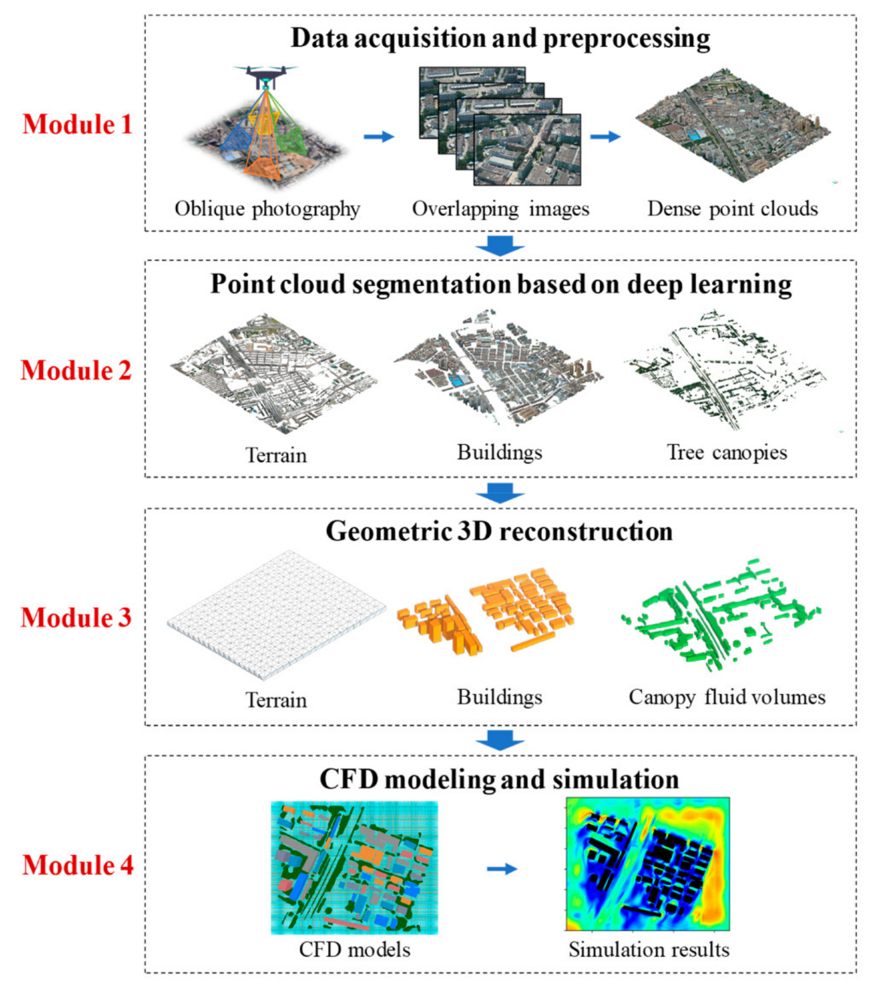
2. Automated Simulation Framework for Urban Wind Environments

As shown in Figure 1, the proposed automated simulation framework for urban wind environments is composed of four modules: (1) data acquisition and preprocessing, (2) point cloud segmentation based on deep learning, (3) geometric 3D reconstruction, and (4) CFD modeling and simulation.
(1) Module 1: data acquisition and preprocessing
In this study, oblique photography is performed to obtain the data needed for modeling. Compared to LiDAR point clouds, the point clouds generated by oblique photography have (a) a lower acquisition cost, (b) a higher density, which is suitable for complex and dense objects in an urban built environment, (c) color information, which enhances the detection of canopies with a significant color feature, and (d) building façade information, which provides more complete object features for deep learning. The aerial trajectory and the camera parameters can be saved during the oblique photography process, and dense point clouds with RGB color information can be generated. Compared with modeling methods using GISs, this method can efficiently and conveniently collect the 3D up-to-date data of a target area and, thus, provide fundamental data support for modeling.
(2) Module 2: point cloud segmentation based on deep learning
Considering the impact of canopies, the CFD simulation of an urban wind environment requires models of the terrain, buildings, and canopy fluid volumes, which are assigned different physical parameters. To establish their respective models, the first step is to perform a semantic segmentation of the point clouds, which divides the point clouds into three parts: terrain, buildings, and tree canopies. A filter is applied to separate the point clouds of the terrain. Subsequently, the point clouds are segmented using deep learning, which remarkably reduces the work of feature engineering and enhances the capture of local features. The method combines the 2D network, DeepLabv3, and the 3D network, PointNet++. The point clouds are first rasterized into 2D images as the input of DeepLabv3, which subsequently predicts the probability vectors of pixel-by-pixel classification and maps them back to the points. Finally, the point clouds are sparsified and input into PointNet++ to obtain point-by-point classification results. Details of this module are elaborated in Section 3.
(3) Module 3: geometric 3D reconstruction
After obtaining the respective point clouds of the terrain, buildings, and tree canopies, it is necessary to establish clean and low-complexity models of the target area, which are suitable for CFD simulation. For the terrain, Gaussian process regression is conducted to fit the elevation of the terrain point clouds, which completes the digital surface model of the area and establishes a 3D model. For buildings, the roof planes are extracted, and their boundaries are detected and refined to form 3D models. For tree canopies, the 2D boundary and height range of each cluster of canopies are determined, and the prisms of the canopy fluid volumes can be established. Finally, the above three parts are integrated, with the overlapping parts eliminated by a Boolean operation. Specific steps relating to this module are introduced in Section 4.
(4) Module 4: CFD modeling and simulation
The 3D models in STL format generated by Module 3 are directly imported into the Phoenics CFD simulation software [47]. Grids are generated using its automatic grid generation function. To perform a CFD simulation of an urban wind environment, the models of the terrain, buildings, and canopy fluid volumes are assigned different physical parameters by implementing an automated script.

3. Point Clouds Separation Based on Deep Learning

3.1. Terrain Filtering

Both terrain and building roofs contain similar horizontal surfaces, which may cause unnecessary misunderstandings in 3D semantic segmentation. The cloth simulation filter (CSF) [48] is applied to the point clouds obtained by oblique photography to extract the terrain point clouds, using a plug-in in the open-source software CloudCompare [48,49].

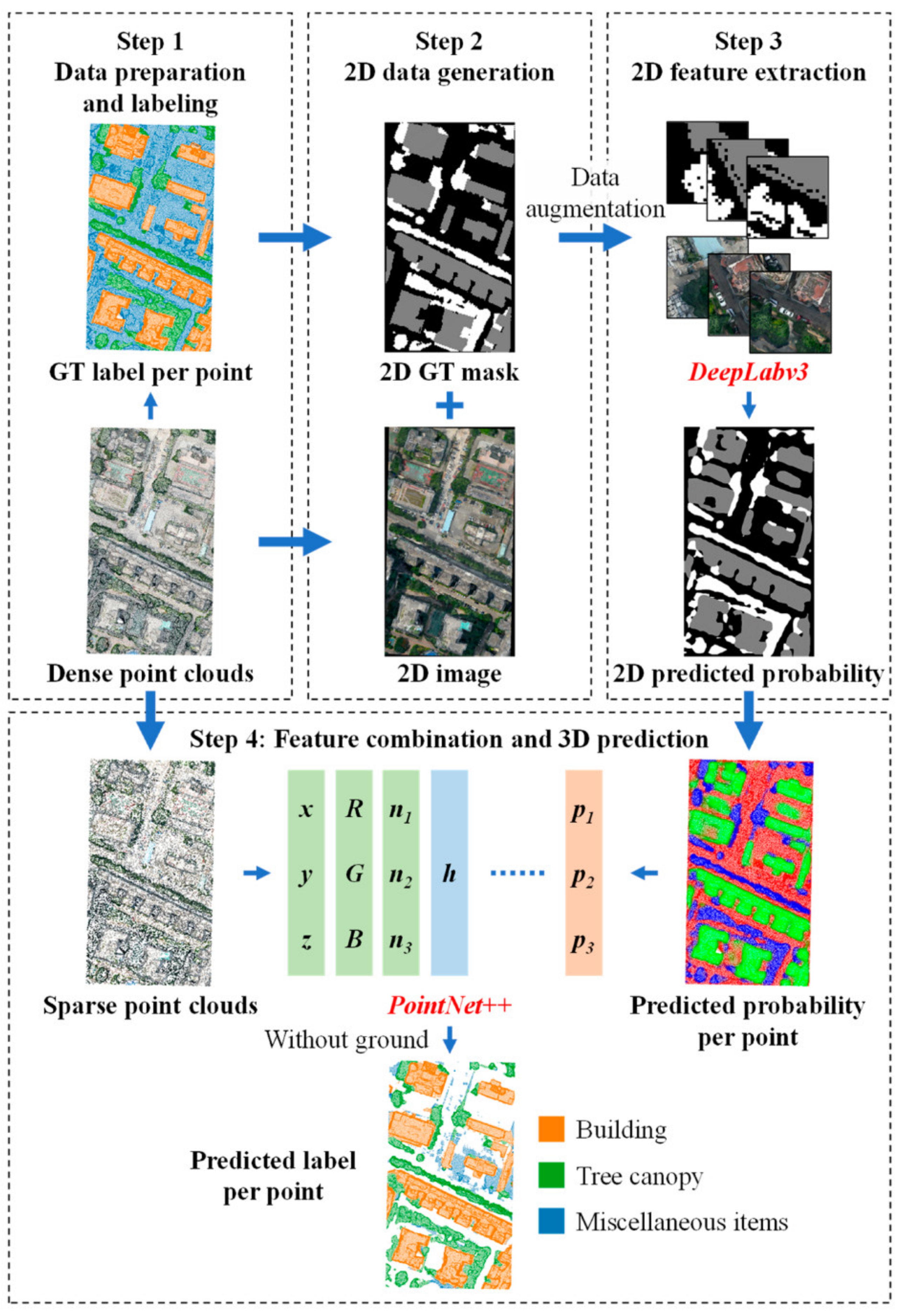
3.2. Segmentation of Buildings and Tree Canopies

As mentioned in Section 1, point cloud segmentation of an urban environment using 2D networks may have limited prediction accuracy at the edges of the objects and cannot reflect 3D features. Although 3D networks overcome the above limitations, they may lose local texture information owing to the limitation of the GPU memory. Moreover, they are more sensitive to the errors in oblique photography point clouds. To overcome the shortcomings of a single 2D or 3D deep learning technique in the point cloud segmentation of an urban environment, both methods are combined to better utilize their respective advantages. The 2D image semantic segmentation network DeepLabv3 [30], which applies an atrous convolution to capture multiscale information, is used. A pre-trained ResNet18 is used as its backbone network. PointNet++ [33], with PointNet [32] as its backbone network, is used as the 3D point cloud semantic segmentation network. It is composed of set-abstraction layers for hierarchical feature extraction and feature-propagation layers for prediction. Using the coordinates and the point-by-point feature vectors as the input, PointNet++ can capture the local characteristics of the point clouds. As shown in Figure 2, the integrated method comprises four steps.
Step 1: data preparation and labeling
In the first step, the dense point clouds are labeled manually, and the dataset is divided into training and test sets as the input of the deep learning networks.
Step 2: 2D data generation
The dense point clouds are projected onto a horizontal plane and rasterized into images. The point set of a tile, which is a point cloud segment of the entire model generated by the oblique photography processing software, is denoted as P . The rasterization process first creates a grid of dimensions H × W over the rectangular bounding area of the tile. Then, an image of the same dimensions H × W is created, and each pixel m , n in the m th row and the n th column corresponds to a grid cell g m , n . Let p P denote a point. The subset of P containing the points in g m , n is denoted as P m , n = p | p P , p   i n   g m , n . The label set of the semantic classes is L = l building , l tree , l misc , whose elements represent buildings, tree canopies, and miscellaneous items, respectively. The RGB color vector, c m , n , of each pixel m , n equals the color vector of the highest point in g m , n , and it restores the aerial top view. c m , n is calculated using Equation (1).
c m , n = c p ,   p = argmax q P m , n z q ,
where c p is the color vector of a point p , and z q is the vertical coordinate of a point q . Similarly, the ground truth label is rasterized into images. The label of each pixel m , n , l m , n , is the label with the most occurrences in g m , n , as expressed in Equation (2).
l m , n = argmax l L q P m , n I l q = l ,
where I · is the counting function with a value of 0 or 1, and l q is the label of a point q . If g m , n does not contain any point, c m , n is calculated by linear interpolation, while l m , n is obtained by the nearest-neighbor interpolation. The data forms required for the 2D image semantic segmentation—2D images and ground truth masks—are thus available.
Step 3: 2D feature extraction
The number of 2D top view images generated by the rasterization is quite small because each tile corresponds to one image only, which is much less than the number of original aerial images directly obtained by a UAV. This amount of data cannot meet the training requirement of DeepLabv3. Therefore, the 2D image data need to be augmented. Random cropping, rotation, and flipping are conducted in this study. After training, DeepLabv3 can produce the probability vectors of the pixel-by-pixel classification, and the length of the vector equals the number of classes, namely L .
Step 4: feature combination and 3D prediction
The dense point clouds are randomly downsampled to a reasonable density based on the capacity of the computing device. The downsampled point clouds have spatial coordinates, RGB colors, and normal vectors. The location relationship between the points and the pixels is determined using the coordinates, and the predicted probability vectors of the pixel-by-pixel classification are mapped to each point. In addition, the relative height of a point is added as one of the features to reflect the vertical characteristics of the objects in the urban environment. The relative height, h p , of a point p is calculated using Equation (3).
h p = z p min q P z q .
The combined feature is a 13-dimensional vector comprising spatial coordinates, RGB colors, normal vectors, 2D predicted probabilities, and a relative height. Only the non-terrain point clouds filtered by the CSF are retained for training and evaluation. PointNet++ yields the point-by-point classification results.
The proposed integrated method has the following three advantages:
(1)
The 2D prediction of DeepLabv3 is combined with the 3D input features of PointNet++, which allows fully utilizing the advantages of the 2D data containing dense texture features and overcomes the shortcoming of the 3D network of losing the local characteristics when the point clouds are sparsified owing to device capacity.
(2)
The z coordinates and the relative heights entailed in PointNet++ strengthen the importance of the vertical information and improve the accuracy at the edges of objects compared to that of the single 2D network.
(3)
The input images of the 2D network are not oblique photos captured by a UAV but are the images rasterized from the projected point clouds. No extra efforts are needed to determine the mapping relationship between the oblique photos and the 3D point clouds. Labeling for training is required only once for the point clouds, which avoids the burden of labeling on 2D images.

4. Geometric 3D Reconstruction

4.1. Terrain Generation

The filtered terrain point clouds, described in Section 3.1, are used to establish a digital surface model. Regular rectangular meshes are applied by fitting the terrain point clouds with the Gaussian process regression model [50].

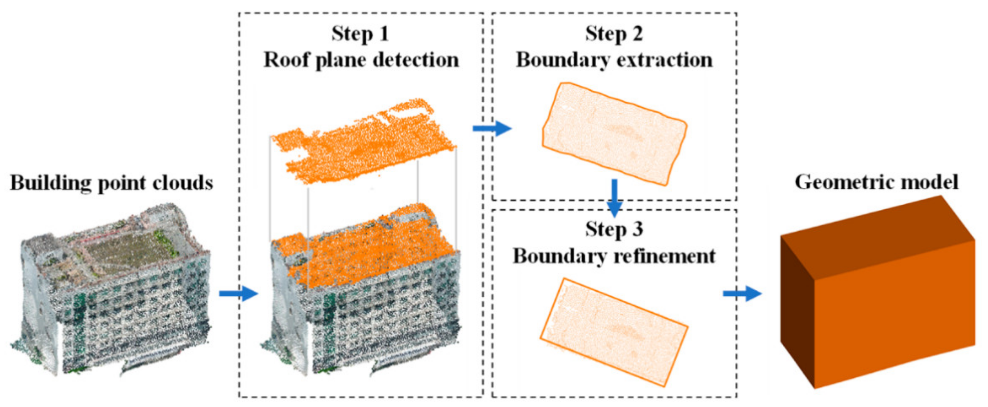
4.2. Building Reconstruction

As shown in Figure 3, the building reconstruction comprises three steps before establishing the geometric models.
Step 1: Roof plane detection
Wang et al. [43] used RANSAC to extract roof planes from airborne LiDAR point clouds. This method is adopted in this study as well. However, different from the technique of Wang et al. [43], in this study, (1) the building point clouds are already separated, as discussed in Section 3.2, which reduces the adverse impact of nonbuilding objects on the extraction of roof planes, (2) oblique photography point clouds are used, which contain the points of building façades; therefore, an angle threshold is set to filter façade planes. RANSAC is implemented using a plug-in of CloudCompare [49,51].
Step 2: Boundary extraction
Constructing 3D models requires the boundary lines of the roof planes. The 2D alpha shape algorithm [37] is adopted to extract the boundaries. To extract reasonable boundaries, the alpha value in the algorithm is adjusted based on the density of the point clouds.
Step 3: Boundary refinement
Owing to the irregularities of building facades and the errors caused by point cloud generation, the boundary geometries may present a zig-zag characteristic after the boundaries are extracted. To create models maintaining general building geometrical and topological features for a CFD simulation, specific steps are taken as follows:
(1)
To address the zig-zag problem, the method proposed by Poullis [52] is adopted, which detects principal directions and regularizes building boundaries based on Gaussian mixture models and energy minimization. The energy minimization problem is equivalent to a minimum cut problem and is solved using gco-v3.0 [53,54,55,56] in this study.
(2)
The Ramer–Douglas–Peucker (RDP) algorithm [57,58] is used to sparsify the boundary points to retain the points that lie along straight lines.
(3)
All boundary line segments in the target area are searched for the segment pairs whose two segments have a distance and an angle within certain thresholds. Subsequently, each segment pair is combined to make both segments in the pair collinear in the horizontal plane.
(4)
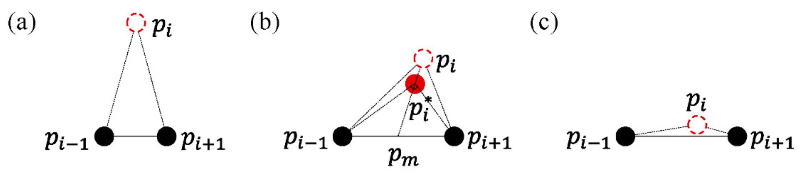
The angle between each adjacent boundary line segment pair of a building is further revised. As shown in Figure 4, for the point set of a building boundary, B , and its sequential points p i 1 , p i , and p i + 1 , based on the threshold, the revision is as follows:
(a)
The extreme acute angles caused by outliers p i are eliminated. The new point set of the building boundary, B * , becomes
B * = B { p i } .
(b)
p i is moved along the median p i p m ¯ of the triangle to p i * when the angle is approximately a right angle. Coordinates x i * of p i * in B * are revised as follows:
m = x i + 1 + x i 1 2   and
x i * = m + 1 2 x i + 1 x i 1 x i m x i m .
(c)
The obtuse angles that are approximately 180° are eliminated to further smoothen the boundary. B * is modified as in Equation (4).
Figure 4. Angle revision of building boundaries for (a) extreme acute angles, (b) approximate right angles, and (c) obtuse angles approximate to 180°.
Remotesensing 13 02383 g004
The 3D reconstruction of buildings is completed using the aforementioned procedure. It should be noted that existing studies have proposed various methods for building reconstruction, among which one feasible technique is adopted in this study. If a method can generate clean and low-complexity building models required for a CFD simulation, it can replace this part of the proposed framework.

4.3. Canopy Fluid Volumes

It is labor-intensive and unnecessary to model each tree in an urban environment for CFD simulations. Amorim et al. [7] grouped neighboring trees and manually modeled each group into a strip-like cuboid, whose height equaled the vertical distance between the average bottom and the average top of canopies in a local area. This can drastically improve the modeling and analysis efficiency and has a limited impact on accuracy [6,7]. In this study, the obtained canopy point clouds are used to build the models of prism-shaped canopy fluid volumes as described in Algorithm 1; specifically,
(1)
The outliers with average distances to neighboring points remarkably larger than the average level in the entire area are removed.
(2)
The point clouds need to be clustered into groups for modeling. Different clustering algorithms have been developed in existing studies [59,60,61]. For the grouping task based on the Euclidean distance, k-means-based algorithms require a pre-specified number of clusters and assume the clusters are convex. Thus, the DBSCAN algorithm [59] is adopted due to its robustness to outliers, explicit control over density via parameters, and variable cluster shapes. The minPoints and eps of DBSCAN are set to 1 and 3.0, respectively, in this study. The groups with a point number less than the threshold are ignored and removed.
(3)
The 2D boundary of each canopy point group is extracted using the 2D alpha shape algorithm [37] and sparsified by the RDP algorithm [57,58].
Algorithm 1. Generation of boundaries of tree canopy volumes
Input: point clouds of tree canopies P tree = { p i | i = 1 , 2 , , k }
Output: set of boundaries of tree canopy volumes B tree
for i 1 to k do
   N p i neighbors p i ,   n        //Set of n-nearest neighbors of p i
   d p i 1 N p i q N p i distance p i , q  //Average distance in N p i
end
P tree { p | p P tree ,   d p 1 k i = 1 k d p i + σ threshold }
T DBSCAN P tree           //Set of clustered point clouds
T { T | T T , T n threshold }
foreach T of T do
   B T AlphaShape 2 D T       //Boundary points of tree canopy T
   B T RDP B T
end
B tree = { B T | T T }

4.4. Postprocessing

The terrain, buildings, and canopy fluid volumes models are integrated. Owing to possible overlap, a Boolean operation is implemented in 3ds Max [62] via a script.

5. Case Study

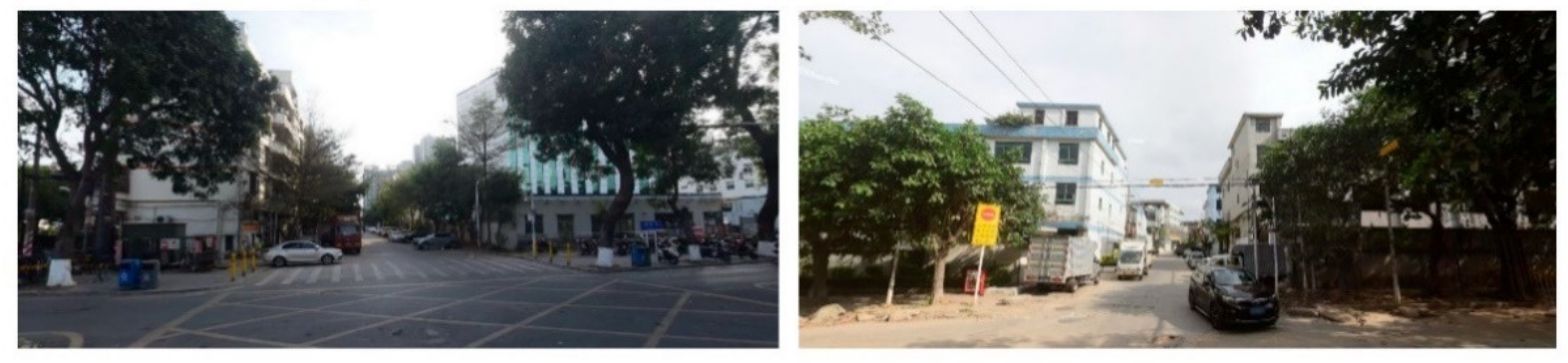
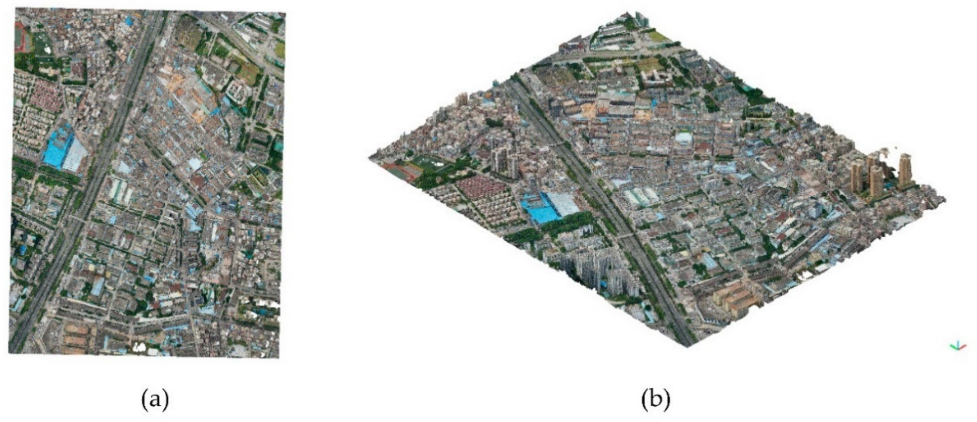
5.1. Case Description

To validate the effectiveness of the proposed automated simulation framework for urban wind environments, a real city is chosen for a case study. Bao’an is an administrative district of Shenzhen, a city in southern China. Various types of buildings are densely built in the district, including residential, industrial, commercial, and other old buildings. In addition, as a typical city in southern China, the city has extensive vegetation, such as street trees. The densely distributed buildings and trees pose a significant challenge to the CFD modeling of its urban environment (Figure 5). By an aerial survey of a local part of Bao’an using a UAV, 3265 photos with a total of 78.4 × 10³ trillion pixels are captured. Thirty tiles of point clouds having similar sizes are generated using ContextCapture [63] (Figure 6). Because oblique photography is easy to implement, the proposed method can better reflect the current environment of the target area than a GIS-based method. The data are labeled by professional students after using the CSF to filter the ground, as shown in Figure 7. The Thirty tiles are rasterized into images for 2D segmentation and feature extraction. The grid size is set to 0.1 m in this study, which approximates the density of the generated point clouds.

5.2. Results and Analysis

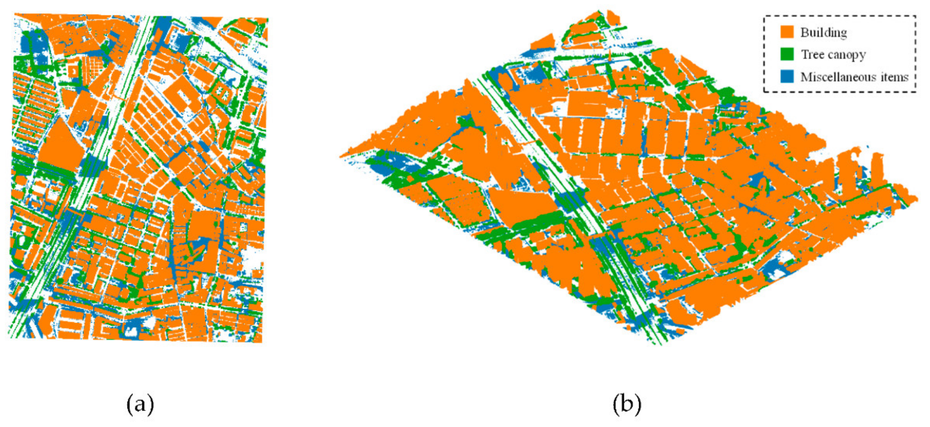
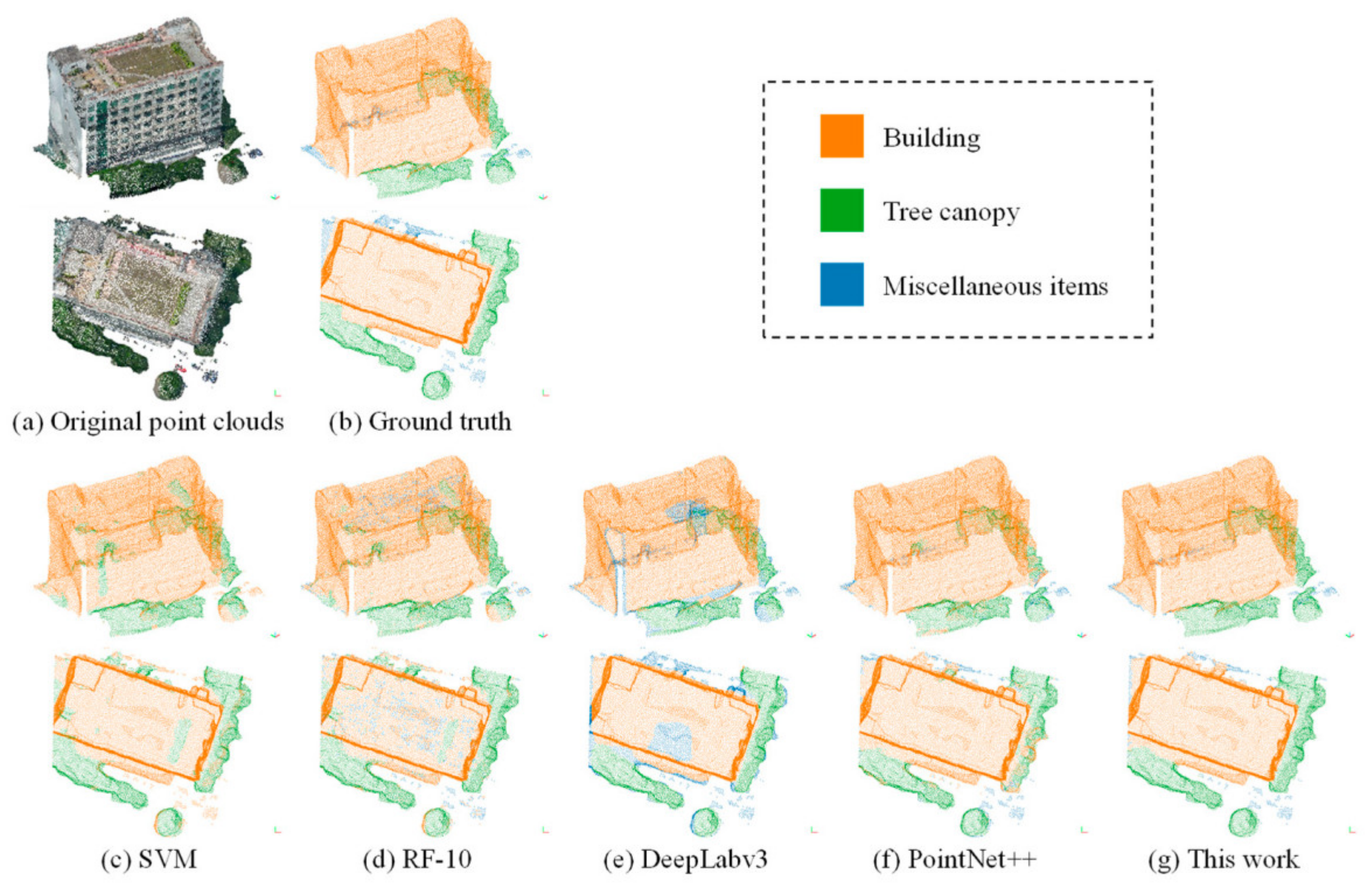
5.2.1. Point Cloud Separation

After the terrain point clouds are filtered by the CSF, the 30 tiles of point clouds are divided in a 6:4 ratio into training and test sets, which contain 18 and 12 tiles, respectively. The prediction accuracies of classification of an SVM, a random forest (RF), DeepLabv3, PointNet++, and the proposed integrated method are compared. The SVM and the RF are implemented based on Scikit-learn [64], while the deep learning techniques are implemented based on PyTorch [65]. The SVM employs the features used by Zhou [24], which describe the regularity, horizontality, flatness, and normal vector distribution. Because Zhou [24] used LiDAR point clouds without color information, a greenness feature, S greenness p [19], is added for the oblique photography point clouds, as expressed in Equation (7).
S greenness p = 1 N p q N p G q R q + G q + B q ,
where N p is the neighborhood point set of a point p and has a range that is consistent with the features used by Zhou [24]. R q , G q , B q is the color vector of a point q . The RF uses the same features as the SVM, and classifiers containing 10, 50, and 100 trees are tested, which are denoted as RF-10, RF-50, and RF-100, respectively.
The backbone network of DeepLabv3 is a ResNet-18 pre-trained on ImageNet. DeepLabv3 applies Atrous Spatial Pyramid Pooling (ASPP) to resample features at different scales. The dilation rates of the kernels (also known as the atrous rates) of the paralleled atrous convolutions are set to (12, 24, 36) in this study. After the augmentation of the original training set through random rotation, flipping, and cropping, the input data of DeepLabv3 comprise 3000 images with a size of 256 × 256. The batch size is 30, and the Adam optimizer with a cosine learning rate initialized at 0.001 is adopted.
PointNet++ uses four set-abstraction layers with single-scale grouping and four feature-propagation layers in this study. The architecture is as follows:
SA(2048, 0.8, [32, 32, 64]) → SA(1024, 1.6, [64, 64, 128]) → SA(512, 3.2, [128, 128, 256]) → SA(256, 6.4, [256, 256, 512]) → FP(256, 256) → FP(256, 256) → FP(256, 128) → FP(128, 128, 128) → FC(128, 0.5) → FC(3)
SA(K, r, [l1, …, ld]) represents a set-abstraction layer with K feature points, a ball query radius r, and d fully connected layers with width li(i = 1, …, d); FP(l1, …, ld) denotes a feature-propagation layer with d fully connected layers; FC(l, rdrop) is a fully connected layer with width l and dropout ratio rdrop. The input data are downsampled to 50,000 points for each tile. The batch size is 6, and the Adam optimizer with a step learning rate initialized at 0.001 is adopted. Readers can refer to [30,33] for more details of the architectures of DeepLabv3 and PointNet++.
The prediction accuracy of the point cloud segmentation is measured in terms of the precision, recall, and F1 score, which are calculated as follows:
p r e c i s i o n = T P T P + F P ,
r e c a l l = T P T P + F N ,   and
F 1 = 2 × p r e c i s i o n × r e c a l l p r e c i s i o n + r e c a l l ,
where T P , F P , and F N denote true positive, false positive, and false negative, respectively. The F1 score is a comprehensive equal-weight metric of precision and recall. Table 1 lists the average metrics achieved on the test set tiles. Taking one building with its surrounding environment as an example, the isometric and top views of the original point clouds, ground truth labels, and predicted labels of the five methods are shown in Figure 8.
It can be concluded that:
(1)
The SVM fails to differentiate between buildings and tree canopies, leading to a misprediction of miscellaneous items (Figure 8c) and relatively low precision for buildings and canopies.
(2)
The RF hardly improves its performance when the number of trees increases but has a slightly higher performance than the SVM; however, there are many outliers mixed in the true classes, which is disadvantageous for the subsequent modeling process.
(3)
Because DeepLabv3 does not have height information, it has a low accuracy at the edges of objects and tends to predict the edge points as miscellaneous items (blue points at the edges of the buildings and the canopies in Figure 8e). This makes the recall higher for miscellaneous items and significantly lower for buildings and canopies compared to their respective precision.
(4)
Although PointNet++ has a satisfying result for buildings, the precision for canopies is low because the normal vector distribution of the canopy areas is irregular. As shown in Figure 8f, the canopy points on the right side of the building have a high probability of being predicted as building points. This may lead to unexpected building point clouds and incomplete canopy point clouds in the modeling step.
(5)
The method proposed in this paper combining DeepLabv3 and PointNet++ improves the accuracy at the edges of objects as well as addresses the problems caused by the complexity of point cloud characteristics and the low generation quality due to occlusion. The accuracy for miscellaneous items is remarkably improved, and the precision and recall of buildings and canopies are balanced well, which can provide accurate point clouds for 3D modeling.

5.2.2. Three-Dimensional Reconstruction

To determine the effects of buildings and tree canopies on the flow field, a local area with densely distributed buildings and trees is selected as the case in the 3D reconstruction and CFD simulation. The selected area is approximately 650 m × 550 m and has 59 buildings in total, with a maximum height of 80 m. The method introduced in Section 4 is utilized to model the terrain, buildings, and canopy fluid volumes, as shown in Figure 9. The models meet the requirement for CFD simulations and retain the geometric features of the main objects to a certain extent. The models are stored in STL format.

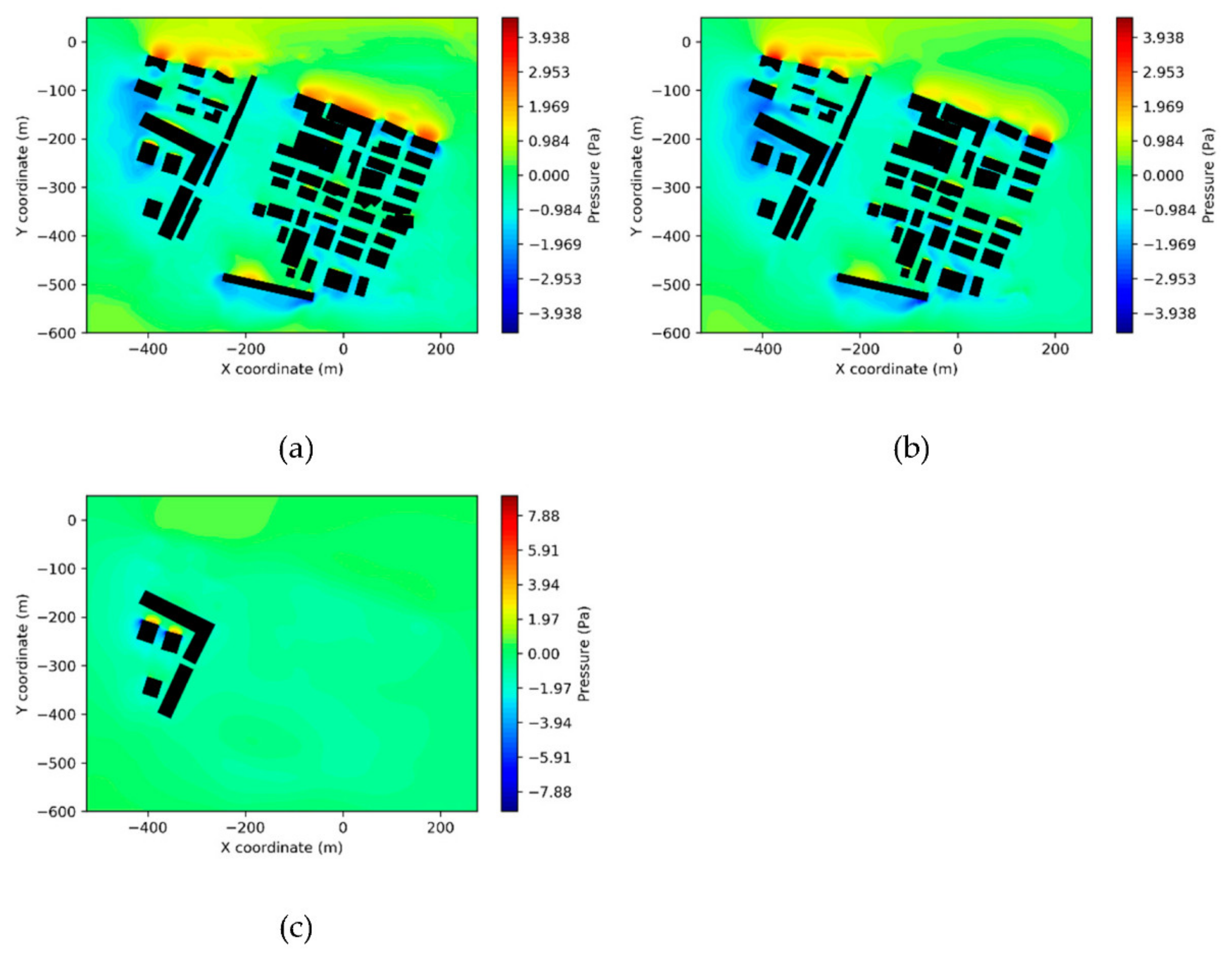
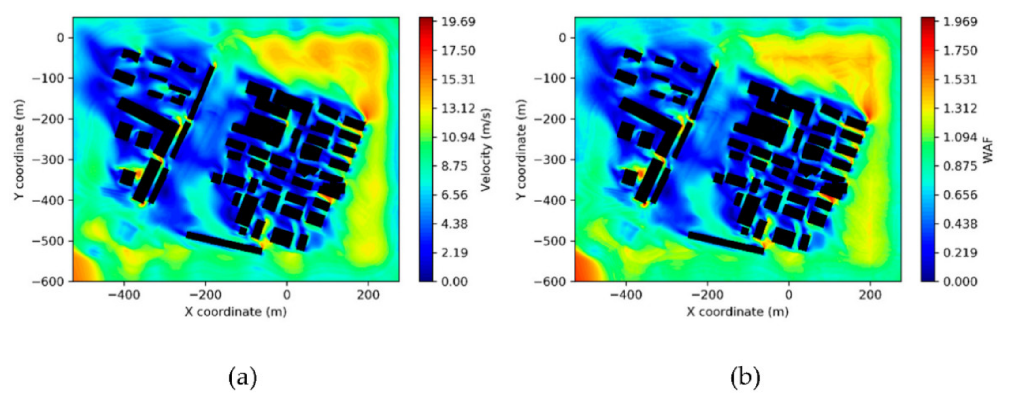
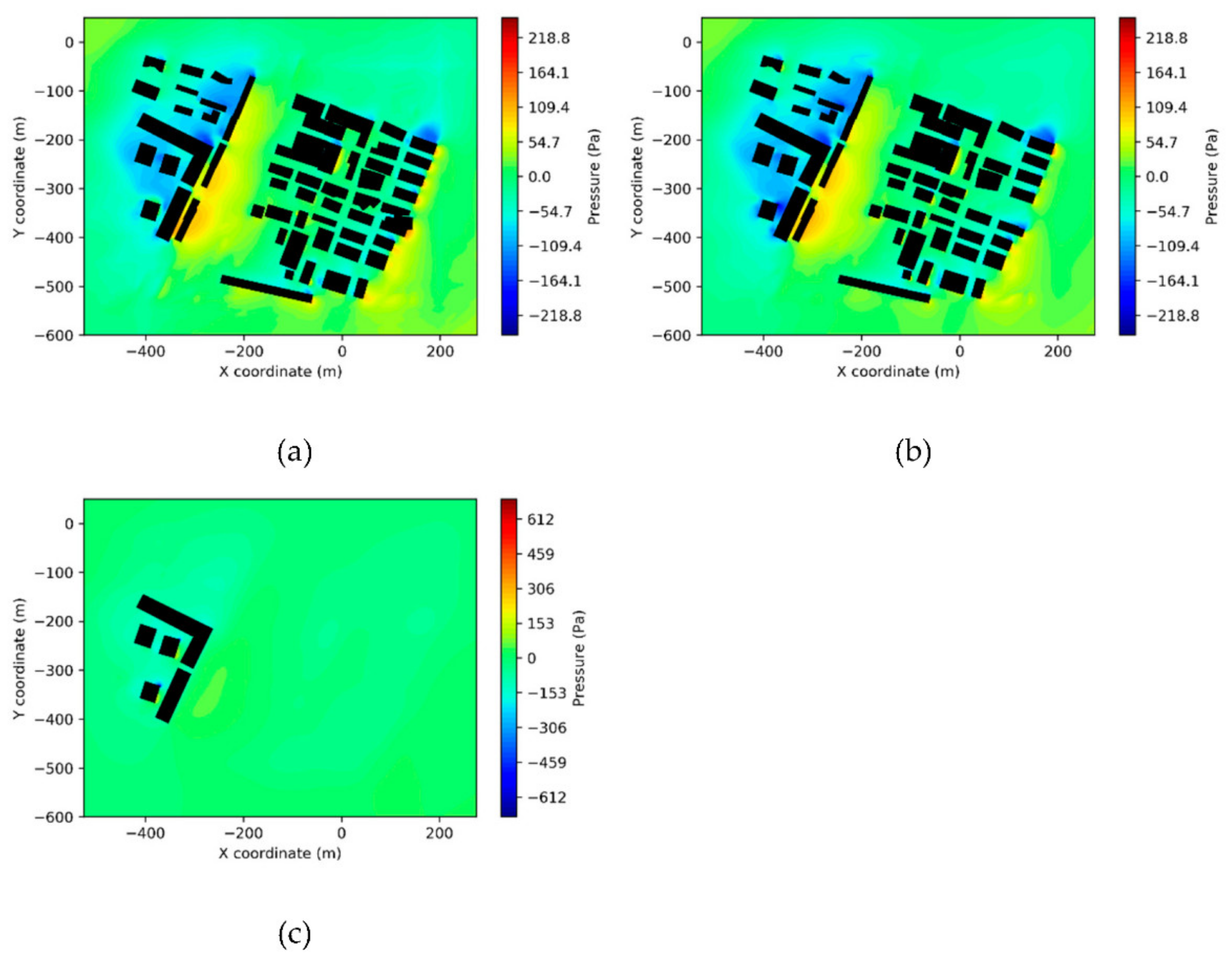
5.2.3. CFD Simulation

The Phoenics CFD simulation software is commonly used for the simulation of outdoor wind environments [66,67,68]; it is easy to use and computationally fast. Therefore, Phoenics is used in this study for the wind simulation of the target area. The generated STL files, described in Section 5.2.2, are directly imported as Phoenics geometric models, as shown in Figure 10a. The domain size is 2300 m × 2300 m × 500 m, which meets the requirements of the distance from domain boundaries to the target area under different wind directions [69]. Adaptive structural grids are generated using the automatic grid-creating function in Phoenics. The grid sizes for the building surfaces can reach approximately 1 m, which meets the requirement for a CFD simulation (Figure 10b).
Typical methods of urban wind environment analysis are adopted when setting the boundary conditions and model parameters in the CFD simulation. The details are provided in Appendix A.
Two scenarios are analyzed in this study.
(1) Annual dominant wind direction
Based on the Shenzhen Climate Bulletin 2019 [70], the annual dominant wind direction is north-northeast (NNE), with a frequency of 17% and an average wind speed of 2.1 m/s at a 10 m reference height. The wind speed, mean age of air, and wind pressure are analyzed under this scenario. The wind amplification factor (WAF) is defined as the local air velocity divided by the wind-profile speed at the local height. The mean age of air represents the time that the air has taken to travel from the domain entry to the local point, and its relative value reflects the degree of air circulation. The height position of the following metrics refers to the height above the ground. Because the model contains a non-planar terrain, the simulation results are extracted in Phoenics using an automatic probe script.
Figure 11 shows the wind speed and the WAF at a pedestrian height of 1.5 m. The whole area is exposed to a wind speed of less than 5 m/s and a WAF of less than 2, which meets the requirements in the Chinese code [71] concerning outdoor walking and comfort. However, because of the dense buildings on the east side and a large L-shaped building on the west side, the wind speed in some internal streets is low and their mean age of air (Figure 12) is higher than that in the surrounding open area. This suggests a poor air circulation condition. Figure 13 shows the wind pressures at 1.5 m, 15 m, and 50 m. Most buildings have a wind pressure difference exceeding 0.5 Pa between their indoor and outdoor environments, which meets the requirements of natural ventilation. Except for the buildings facing streets and the top stories of the west-side tall buildings, the wind pressure difference between the windward and leeward sides meets the requirement of not exceeding 5 Pa [71].
(2) Tropical storm
In 2019, Shenzhen experienced the tropical storm Wipha, which exhibited a wind speed of 14.1 m/s at a 10 m reference height [70]. The dominant wind direction was southeast (SE). The wind speed and pressure are analyzed under this scenario.
Figure 14 shows the wind speed and WAF at 1.5 m. Because the wind direction is close to the street direction inside the area, a significant wind amplification effect is observed near the street entrance, which makes pedestrian walking difficult. The wind pressures at 1.5 m, 15 m, and 50 m are shown in Figure 15. Under the tropical storm, some of the buildings facing streets experience a large pressure difference between the windward and leeward sides, which increases the risk of falling debris and thus requires attention.

6. Discussion

6.1. Data Acquisition and Errors

The proposed framework adopts digital aerial photogrammetry as its data acquisition approach, considering that its cost is significantly lower than that of airborne laser scanning (ALS) using LiDAR [72]. That would enable a frequent implementation of the proposed method to consider changes in the CFD models. Nevertheless, noises exist in the point clouds generated by oblique photography due to reasons such as occlusion, parallax, texture loss, and lighting conditions [73]. Many studies have lain their emphasis on the issue of data noise [74,75]. However, common noise filtering algorithms for point clouds, such as statistical outlier removal and radius outlier removal, significantly rely on parameter settings. Unreasonable parameters would cause the point clouds to be sparse and thus lose geometric information. Since data noise is not the focus of this work, no noise filtering is applied before the semantic segmentation module to avoid an adverse effect on the local feature learning of the following classification models. Although the noise is not filtered in advance, the proposed method can be robust to outliers. That is because both the feature calculation required by SVM/RF and the ASPP(DeepLabv3)/SA(PointNet++) layer perform local feature extractions, which implicitly help identify the outliers. On the other hand, the building reconstruction first applies RANSAC to extract roof planes, equivalently performing a plane-wise outlier filtering. As for trees, the model of canopy fluid volumes is generated by the 2D alpha shape algorithm, making the detected boundary more sensitive to outliers than internal sparseness. Therefore, an outlier removal is performed in Algorithm 1. The noise of point clouds might also be brought by systematic errors. Gopalakrishnan et al. [76] used ALS data to address the vertical misregistration issue of the photogrammetry-based point clouds. This kind of method would be able to reduce the data noise, whose impact on the proposed method needs further study.

6.2. Efficiency

The segmentation experiment is carried out on a high-performance computer. The device is equipped with an Intel Xeon E5-2630 v3 @ 2.40GHz as CPU, an NVIDIA GeForce GTX1080 as GPU, and 64 GB RAM. The system is Ubuntu 20.04. The time cost of the proposed method mainly consists of two parts: the calculation time of DeepLabv3 and PointNet++. In the case study, the time cost is 1664 s during training, while being 147 s for the test. In comparison, the single DeepLabv3 method costs 344 s and 126 s for training and test respectively, while the figures for PointNet++ are 1316 s and 21 s. The SVM and RF methods spend a lot of time on point-wise feature calculation, which is 1377 s and 879 s for the training set and the test set, respectively. The training time for SVM is 221 s, while its test time is 0.1 s which can be ignored. As for RF, the training time is 191 s, 967 s, and 1939 s for RF with 10, 50, and 100 trees, respectively, while the test process costs 27 s, 124 s, and 261 s. It should be noted that the figures above are based on the same training and test set, and do not take into account the time for file I/O required by the implementation of the framework. In addition, the deep learning techniques leverage the GPU, while SVM and RF only use the CPU.
Although the proposed segmentation method slightly costs more time for an accuracy improvement, the time efficiency is competent in terms of the entire modeling framework. In the case study, using the point cloud segmentation and model reconstruction methods presented in this study, the CFD models are established by the well-trained model within minutes for a complex urban area including vegetation on a personal computer, saving hours of professional manual works on establishing the up to date as-built models. The CFD simulation considers complex buildings, vegetation, and their interaction effects. The proposed method significantly reduces the labor cost of CFD modeling of an urban wind environment, and professionals can focus more on the simulation and result analyses, which is surely beneficial to applications in wind disasters, such as fragility analysis, risk analysis, and decision making.

6.3. Geometric Quality

The geometric quality of the model is critical to an accurate CFD result. For the ground model, Gaussian process regression is used to reconstruct the digital surface model. If the accuracy needs to be improved, the sampling density on the surface can be increased, or methods such as Poisson surface reconstruction can be applied to build a high-precision surface. For building models, this work adopts common implementations in relevant regional simulation studies in terms of the level of detail [6,7]. Hågbo et al. [41] also showed that the adopted level of detail would have a limited impact on decision-making using wind environment analysis results. For canopy fluid volumes, Gu et al. [6] used the field measurement data to validate the model without vertical geometric changes, and the results showed that the simulation outcomes of the wind speed are within a standard deviation of the measurement. Thus, such a model is adopted in this work for simplicity. Normally, by increasing the level of details of the models, such as using building models established by the mesh surface reconstruction and canopy fluid models built hierarchically to consider vertical changes, the simulation accuracy would be enhanced. However, this would reduce modeling efficiency and result in higher requirements for the CFD meshing, which needs more numerical verifications.

7. Conclusions

CFD is an effective tool for the simulation of urban wind environments and can be employed to wind disaster analysis. A CFD simulation requires accurately and efficiently establishing clean and low-complexity models of a city, including terrain, buildings, and vegetation. This paper proposes an automated simulation framework for urban wind environments based on aerial point clouds and deep learning, and mainly focuses on the modeling process. The practicality of the framework is validated by a case study on Bao’an, Shenzhen. The main conclusions are as follows:
(1)
Compared with the traditional CFD modeling methods based on GISs, the automated method based on oblique photography point clouds can reflect the current environment of the target area and drastically reduce the labor cost.
(2)
Compared to the point cloud semantic segmentation methods based on SVM, RF, or a single deep learning network, the proposed method combining 2D and 3D deep learning techniques achieves a higher accuracy, which provides more accurate classification results for the modeling process.
(3)
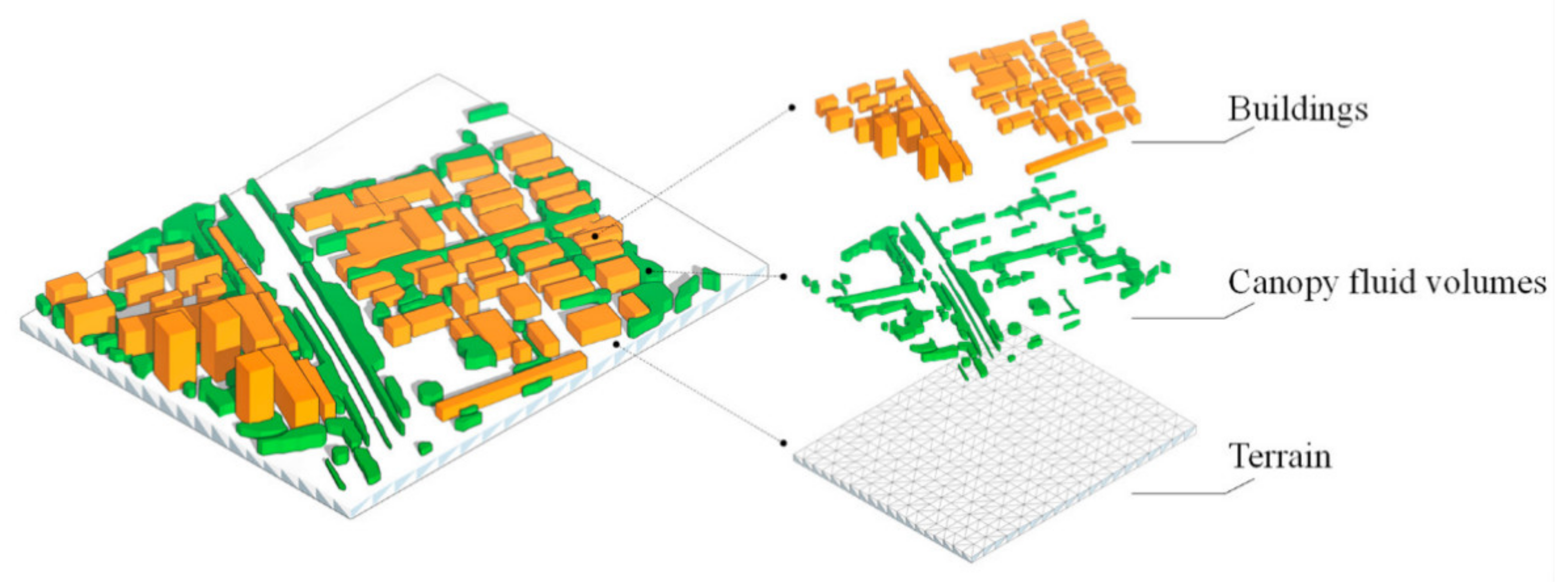
The modeling method of the terrain, buildings, and canopy fluid volumes can retain general geometric characteristics of the objects while reducing the model complexity, which meets the requirements of CFD simulations.

Author Contributions

Conceptualization, X.L., F.Z. and C.S.; methodology, C.S.; software, C.S.; validation, P.Z.; data curation, X.Z.; writing—original draft preparation, C.S.; writing—review and editing, X.L. and Y.H.; funding acquisition, X.L. All authors have read and agreed to the published version of the manuscript.

Funding

This research was funded by the Central Research Institute of Building and Construction Co., Ltd., MCC Group, China (No. YYY2020Z047), and Tencent Foundation through XPLORER PRIZE.

Acknowledgments

The authors would like to appreciate Beijing PARATERA Tech Co., Ltd. for providing the computational support in this work, and also the anonymous reviewers for the constructive suggestions.

Conflicts of Interest

The authors declare no conflict of interest.

Appendix A

The inlet boundary is set as a velocity inlet and uses the power-law wind profile, as expressed in Equation (A1).
U z = U r z z r α ,
where z r and U r represent the z coordinate and wind speed at the reference position, respectively; z r is typically 10 m, and α is the power-law exponent, which is set as 0.22 for an urban area with dense buildings according to the Chinese code [8]. The surfaces of the terrain and buildings are set as nonslip boundaries and wall functions. Other domain boundaries are set as fixed-pressure boundaries. The Reynolds-averaged Navier–Stokes (RANS) model and the Chen–Kim k–ε turbulence model [77] are adopted for the computation.
The main impact of trees on the wind field is the reduction in the wind speed due to the drag forces and the additional turbulence levels produced by the canopies. These effects are simulated by adding a sink term to the momentum equation and source terms to the transport equations of k and ε . Equations (A2)–(A5) are the RANS equations of the incompressible flow used in the simulation. For the notations, the Einstein summation convention is used as follows:
u i x i = 0 ,
u j u i x j = 1 ρ p x i + x j ν + ν t u i x j + u j x i 2 3 k δ i j + S d ,
x i k u i = x j ν + ν t σ k k x j + ν t u i x j + u j x i u i x j ε + S k ,   and
x i ε u i = x j ν + ν t σ ε ε x j + C 1 ε ε k ν t u i x j + u j x i u i x j C 2 ε ε 2 k + S ε C K + S ε ,  
where u i is the velocity (where i equals 1, 2, or 3), x i denotes the spatial coordinates, ρ is the density; p is the pressure, δ i j represents the Kronecker delta, ν is the viscosity, and ν t is the eddy viscosity, which can be calculated based on the kinetic energy, k , and the turbulent energy dissipation rate, ε [78], as follows:
ν t = C μ k 2 ε .
S ε C K is the source term introduced by Chen and Kim [77].
S ε C K = C 4 ε k ν t u i x j + u j x i u i x j 2 .
S d is the sink term associated with the drag forces of the tree canopies, and S k and S ε are the source terms introduced to account for the turbulent interaction between the airflow and the tree canopies.
S d = C d α u u i ,
S k = C d α β p u 3 β d u k ,   and
S ε = C d α C 5 ε β p u 3 ε k C 6 ε β d u ε ,
where α is the leaf area density (LAD), and u is the scalar value of the velocity vector. Various studies have proposed different parameter values to consider the influence of tree canopies [79,80,81,82]; the value suggested by Green [79] is adopted in this study. Because of the lack of detailed data on vegetation, the LAD is typically 4.0 and is assumed to be vertically invariant [83], and the drag coefficient, C d , is set as 0.2 [7]. The constants used in the numerical equations are listed in Table A1.
Table A1. Constants used in numerical equations for modeling effects of trees on airflow.
C μ σ k σ ε C 1 ε C 2 ε C 4 ε C 5 ε C 6 ε β p β d C d α
0.090.751.151.151.90.251.501.501.004.000.204.00

References

  1. Blocken, B. Computational Fluid Dynamics for Urban Physics: Importance, Scales, Possibilities, Limitations and Ten Tips and Tricks towards Accurate and Reliable Simulations. Build. Environ. 2015, 91, 219–245. [Google Scholar] [CrossRef] [Green Version]
  2. Zhang, Y.; Wei, K.; Shen, Z.; Bai, X.; Lu, X.; Soares, C.G. Economic Impact of Typhoon-Induced Wind Disasters on Port Operations: A Case Study of Ports in China. Int. J. Disaster Risk Reduct. 2020, 50, 101719. [Google Scholar] [CrossRef]
  3. Song, B.; Galasso, C.; Garciano, L. Wind-Uplift Fragility Analysis of Roof Sheathing for Cultural Heritage Assets in the Philippines. Int. J. Disaster Risk Reduct. 2020, 51, 101753. [Google Scholar] [CrossRef]
  4. Schulman, L.L.; DesAutels, C.G. Computational Fluid Dynamics Simulations to Predict Wind-Induced Damage to a Steel Building during Hurricane Katrina. In Forensic Engineering 2012; American Society of Civil Engineers: San Francisco, CA, USA, 2012; pp. 793–800. [Google Scholar] [CrossRef]
  5. Blocken, B.; Janssen, W.D.; van Hooff, T. CFD Simulation for Pedestrian Wind Comfort and Wind Safety in Urban Areas: General Decision Framework and Case Study for the Eindhoven University Campus. Environ. Model. Softw. 2012, 30, 15–34. [Google Scholar] [CrossRef]
  6. Gu, D.; Zhao, P.; Chen, W.; Huang, Y.; Lu, X. Near Real-Time Prediction of Wind-Induced Tree Damage at a City Scale: Simulation Framework and Case Study for Tsinghua University Campus. Int. J. Disaster Risk Reduct. 2021, 53, 102003. [Google Scholar] [CrossRef]
  7. Amorim, J.H.; Rodrigues, V.; Tavares, R.; Valente, J.; Borrego, C. CFD Modelling of the Aerodynamic Effect of Trees on Urban Air Pollution Dispersion. Sci. Total. Environ. 2013, 461, 541–551. [Google Scholar] [CrossRef] [PubMed]
  8. Ministry of Housing and Urban-Rural Development of the People’s Republic of China. Standard for Green Performance Calculation of Civil. Buildings (JGJ/T 449-2018); China Architecture & Building Press: Beijing, China, 2018.
  9. Gu, D.; Zheng, Z.; Zhao, P.; Xie, L.; Xu, Z.; Lu, X. High-Efficiency Simulation Framework to Analyze the Impact of Exhaust Air from COVID-19 Temporary Hospitals and Its Typical Applications. Appl. Sci. 2020, 10, 3949. [Google Scholar] [CrossRef]
  10. Dalla Mura, M.; Prasad, S.; Pacifici, F.; Gamba, P.; Chanussot, J.; Benediktsson, J.A. Challenges and Opportunities of Multimodality and Data Fusion in Remote Sensing. Proc. IEEE 2015, 103, 1585–1601. [Google Scholar] [CrossRef] [Green Version]
  11. Jochem, W.C.; Bird, T.J.; Tatem, A.J. Identifying Residential Neighbourhood Types from Settlement Points in a Machine Learning Approach. Comput. Environ. Urban. Syst. 2018, 69, 104–113. [Google Scholar] [CrossRef]
  12. Hecht, R.; Meinel, G.; Buchroithner, M. Automatic Identification of Building Types Based on Topographic Databases—A Comparison of Different Data Sources. Int. J. Cartogr. 2015, 1, 18–31. [Google Scholar] [CrossRef] [Green Version]
  13. Shirowzhan, S.; Sepasgozar, S.M.E.; Li, H.; Trinder, J.; Tang, P. Comparative Analysis of Machine Learning and Point-Based Algorithms for Detecting 3D Changes in Buildings over Time Using Bi-Temporal Lidar Data. Autom. Constr. 2019, 105, 102841. [Google Scholar] [CrossRef]
  14. Chen, J.; Tang, P.; Rakstad, T.; Patrick, M.; Zhou, X. Augmenting a Deep-Learning Algorithm with Canal Inspection Knowledge for Reliable Water Leak Detection from Multispectral Satellite Images. Adv. Eng. Inform. 2020, 46, 101161. [Google Scholar] [CrossRef]
  15. Cooner, A.J.; Shao, Y.; Campbell, J.B. Detection of Urban Damage Using Remote Sensing and Machine Learning Algorithms: Revisiting the 2010 Haiti Earthquake. Remote. Sens. 2016, 8, 868. [Google Scholar] [CrossRef] [Green Version]
  16. Gomez, C.; Purdie, H. UAV-Based Photogrammetry and Geocomputing for Hazards and Disaster Risk Monitoring—A Review. Geoenviron. Disasters 2016, 3, 23. [Google Scholar] [CrossRef] [Green Version]
  17. Xiong, C.; Li, Q.; Lu, X. Automated Regional Seismic Damage Assessment of Buildings Using an Unmanned Aerial Vehicle and a Convolutional Neural Network. Autom. Constr. 2020, 109, 102994. [Google Scholar] [CrossRef]
  18. Zhou, Y.; Wang, L.; Love, P.E.D.; Ding, L.; Zhou, C. Three-Dimensional (3D) Reconstruction of Structures and Landscapes: A New Point-and-Line Fusion Method. Adv. Eng. Inform. 2019, 42, 100961. [Google Scholar] [CrossRef]
  19. Sun, X.; Shen, S.; Hu, Z. Automatic Building Extraction from Oblique Aerial Images. In Proceedings of the 2016 23rd International Conference on Pattern Recognition (ICPR), Cancun, Mexico, 4–8 December 2016; pp. 663–668. [Google Scholar] [CrossRef]
  20. Tomljenovic, I.; Tiede, D.; Blaschke, T. A Building ExSegmentation of Airborne Point Cloud Data for Autcanner Data Utilizing the Object Based Image Analysis Paradigm. Int. J. Appl. Earth Obs. Geoinf. 2016, 52, 137–148. [Google Scholar] [CrossRef] [Green Version]
  21. Gilani, S.A.N.; Awrangjeb, M.; Lu, G. Segmentation of Airborne Point Cloud Data for Automatic Building Roof Extraction. GISci. Remote. Sens. 2018, 55, 63–89. [Google Scholar] [CrossRef] [Green Version]
  22. Verma, V.; Kumar, R.; Hsu, S. 3D Building Detection and Modeling from Aerial LIDAR Data. In Proceedings of the 2006 IEEE Computer Society Conference on Computer Vision and Pattern Recognition (CVPR’06), New York, NY, USA, 17–22 June 2006; Volume 2, pp. 2213–2220. [Google Scholar] [CrossRef]
  23. Anuar, S.F.K.; Nasir, A.A.M.; Azri, S.; Ujang, U.; Majid, Z.; González Cuétara, M.; de Miguel Retortillo, G. 3D Geometric Extraction Using Segmentation for Asset Management. In The International Archives of the Photogrammetry, Remote Sensing and Spatial Information Sciences; Copernicus GmbH: Göttingen, Germany, 2020; Volume XLIV-4-W3-2020, pp. 61–69. [Google Scholar] [CrossRef]
  24. Zhou, Q. 3D Urban Modeling from City-Scale Aerial LiDAR Data. Ph.D. Thesis, University of Southern California, Los Angeles, CA, USA, 2012. [Google Scholar]
  25. Rida, I.; Almaadeed, N.; Almaadeed, S. Robust Gait Recognition: A Comprehensive Survey. IET Biom. 2019, 8, 14–28. [Google Scholar] [CrossRef]
  26. Long, J.; Shelhamer, E.; Darrell, T. Fully Convolutional Networks for Semantic Segmentation. In Proceedings of the 2015 IEEE Conference on Computer Vision and Pattern Recognition (CVPR), Boston, MA, USA, 7–12 June 2015; pp. 3431–3440. [Google Scholar] [CrossRef] [Green Version]
  27. Ronneberger, O.; Fischer, P.; Brox, T. U-Net: Convolutional Networks for Biomedical Image Segmentation. In Medical Image Computing and Computer-Assisted Intervention—MICCAI 2015; Springer International Publishing: Cham, Switzerland, 2015; pp. 234–241. [Google Scholar] [CrossRef] [Green Version]
  28. Chen, L.-C.; Papandreou, G.; Kokkinos, I.; Murphy, K.; Yuille, A.L. Semantic Image Segmentation with Deep Convolutional Nets and Fully Connected CRFs. arXiv 2016, arXiv:1412.7062. [Google Scholar]
  29. Chen, L.-C.; Papandreou, G.; Kokkinos, I.; Murphy, K.; Yuille, A.L. DeepLab: Semantic Image Segmentation with Deep Convolutional Nets, Atrous Convolution, and Fully Connected CRFs. IEEE Trans. Pattern Anal. Mach. Intell. 2018, 40, 834–848. [Google Scholar] [CrossRef] [PubMed]
  30. Chen, L.-C.; Papandreou, G.; Schroff, F.; Adam, H. Rethinking Atrous Convolution for Semantic Image Segmentation. arXiv 2017, arXiv:1706.05587. [Google Scholar]
  31. Maturana, D.; Scherer, S. VoxNet: A 3D Convolutional Neural Network for Real-Time Object Recognition. In Proceedings of the 2015 IEEE/RSJ International Conference on Intelligent Robots and Systems (IROS), Hamburg, Germany, 28 September–2 October 2015; pp. 922–928. [Google Scholar] [CrossRef]
  32. Qi, C.R.; Su, H.; Mo, K.; Guibas, L.J. PointNet: Deep Learning on Point Sets for 3D Classification and Segmentation. In Proceedings of the 2017 IEEE Conference on Computer Vision and Pattern Recognition (CVPR), Honolulu, HI, USA, 21–26 July 2017; pp. 77–85. [Google Scholar] [CrossRef] [Green Version]
  33. Qi, C.R.; Yi, L.; Su, H.; Guibas, L.J. PointNet++: Deep Hierarchical Feature Learning on Point Sets in a Metric Space. In Proceedings of the 31st International Conference on Neural Information Processing Systems, Long Beach, CA, USA, 4–9 December 2017; Curran Associates Inc.: Red Hook, NY, USA, 2017; pp. 5105–5114. [Google Scholar]
  34. Zhang, Y.; Huo, K.; Liu, Z.; Zang, Y.; Liu, Y.; Li, X.; Zhang, Q.; Wang, C. PGNet: A Part-Based Generative Network for 3D Object Reconstruction. Knowl. Based Syst. 2020, 194, 105574. [Google Scholar] [CrossRef]
  35. Kim, H.; Yoon, J.; Sim, S.-H. Automated Bridge Component Recognition from Point Clouds Using Deep Learning. Struct. Control. Health Monit. 2020, 27, e2591. [Google Scholar] [CrossRef]
  36. Lowphansirikul, C.; Kim, K.; Vinayaraj, P.; Tuarob, S. 3D Semantic Segmentation of Large-Scale Point-Clouds in Urban Areas Using Deep Learning. In Proceedings of the 2019 11th International Conference on Knowledge and Smart Technology (KST), Phuket, Thailand, 23–26 January 2019; pp. 238–243. [Google Scholar] [CrossRef]
  37. Edelsbrunner, H.; Kirkpatrick, D.; Seidel, R. On the Shape of a Set of Points in the Plane. IEEE Trans. Inf. Theory 1983, 29, 551–559. [Google Scholar] [CrossRef] [Green Version]
  38. Bernardini, F.; Mittleman, J.; Rushmeier, H.; Silva, C.; Taubin, G. The Ball-Pivoting Algorithm for Surface Reconstruction. IEEE Trans. Vis. Comput. Graph. 1999, 5, 349–359. [Google Scholar] [CrossRef]
  39. Kazhdan, M.; Bolitho, M.; Hoppe, H. Poisson Surface Reconstruction. In Proceedings of the 4th Eurographics Symposium on Geometry Processing, Sardinia, Italy, 26–28 June 2006; Eurographics Association: Goslar, Germany, 2006; pp. 61–70. [Google Scholar]
  40. Xu, Z.; Wu, Y.; Lu, X.; Jin, X. Photo-Realistic Visualization of Seismic Dynamic Responses of Urban Building Clusters Based on Oblique Aerial Photography. Adv. Eng. Inform. 2020, 43, 101025. [Google Scholar] [CrossRef]
  41. Hågbo, T.-O.; Giljarhus, K.E.T.; Hjertager, B.H. Influence of Geometry Acquisition Method on Pedestrian Wind Simulations. arXiv 2020, arXiv:2010.12371. [Google Scholar]
  42. Chen, L.; Teo, T.; Rau, J.; Liu, J.; Hsu, W. Building Reconstruction from LIDAR Data and Aerial Imagery. In Proceedings of the 2005 IEEE International Geoscience and Remote Sensing Symposium, 2005. (IGARSS ’05), Seoul, Korea, 29–29 July 2005; Volume 4, pp. 2846–2849. [Google Scholar] [CrossRef]
  43. Wang, X.; Chan, T.O.; Liu, K.; Pan, J.; Luo, M.; Li, W.; Wei, C. A Robust Segmentation Framework for Closely Packed Buildings from Airborne LiDAR Point Clouds. Int. J. Remote. Sens. 2020, 41, 5147–5165. [Google Scholar] [CrossRef]
  44. Lu, X.; Guo, Q.; Li, W.; Flanagan, J. A Bottom-up Approach to Segment Individual Deciduous Trees Using Leaf-off Lidar Point Cloud Data. ISPRS J. Photogramm. Remote. Sens. 2014, 94, 1–12. [Google Scholar] [CrossRef]
  45. Lin, Y.; Jiang, M.; Yao, Y.; Zhang, L.; Lin, J. Use of UAV Oblique Imaging for the Detection of Individual Trees in Residential Environments. Urban. For. Urban. Green. 2015, 14, 404–412. [Google Scholar] [CrossRef]
  46. Wang, Y.; Weinacker, H.; Koch, B. A Lidar Point Cloud Based Procedure for Vertical Canopy Structure Analysis and 3D Single Tree Modelling in Forest. Sensors 2008, 8, 3938–3951. [Google Scholar] [CrossRef] [PubMed] [Green Version]
  47. Phoenics. Available online: http://www.cham.co.uk/phoenics.php (accessed on 5 January 2021).
  48. Zhang, W.; Qi, J.; Wan, P.; Wang, H.; Xie, D.; Wang, X.; Yan, G. An Easy-to-Use Airborne LiDAR Data Filtering Method Based on Cloth Simulation. Remote. Sens. 2016, 8, 501. [Google Scholar] [CrossRef]
  49. CloudCompare: 3D Point Cloud and Mesh Processing Software, Open Source Project. Available online: https://www.danielgm.net/cc/ (accessed on 30 November 2020).
  50. Vasudevan, S.; Ramos, F.; Nettleton, E.; Durrant-Whyte, H.; Blair, A. Gaussian Process Modeling of Large Scale Terrain. In Proceedings of the 2009 IEEE International Conference on Robotics and Automation, Kobe, Japan, 12–17 May 2009; pp. 1047–1053. [Google Scholar] [CrossRef]
  51. Schnabel, R.; Wahl, R.; Klein, R. Efficient RANSAC for Point-Cloud Shape Detection. Comput. Graph. Forum 2007, 26, 214–226. [Google Scholar] [CrossRef]
  52. Poullis, C. A Framework for Automatic Modeling from Point Cloud Data. IEEE Trans. Pattern Anal. Mach. Intell. 2013, 35, 2563–2575. [Google Scholar] [CrossRef] [PubMed]
  53. Boykov, Y.; Veksler, O.; Zabih, R. Fast Approximate Energy Minimization via Graph Cuts. IEEE Trans. Pattern Anal. Mach. Intell. 2001, 23, 1222–1239. [Google Scholar] [CrossRef] [Green Version]
  54. Kolmogorov, V.; Zabin, R. What Energy Functions Can Be Minimized via Graph Cuts? IEEE Trans. Pattern Anal. Mach. Intell. 2004, 26, 147–159. [Google Scholar] [CrossRef] [Green Version]
  55. Boykov, Y.; Kolmogorov, V. An Experimental Comparison of Min-Cut/Max- Flow Algorithms for Energy Minimization in Vision. IEEE Trans. Pattern Anal. Mach. Intell. 2004, 26, 1124–1137. [Google Scholar] [CrossRef] [Green Version]
  56. Delong, A.; Osokin, A.; Isack, H.N.; Boykov, Y. Fast Approximate Energy Minimization with Label Costs. Int. J. Comput. Vis. 2012, 96, 1–27. [Google Scholar] [CrossRef]
  57. Ramer, U. An Iterative Procedure for the Polygonal Approximation of Plane Curves. Comput. Graph. Image Process. 1972, 1, 244–256. [Google Scholar] [CrossRef]
  58. Douglas, D.; Peucker, T. Algorithms for the Reduction of the Number of Points Required to Represent a Digitized Line or Its Caricature. Cartogr. Int. J. Geogr. Inf. Geovisualization 1973, 10, 112–122. [Google Scholar] [CrossRef] [Green Version]
  59. Ester, M.; Kriegel, H.-P.; Sander, J.; Xu, X. A Density-Based Algorithm for Discovering Clusters in Large Spatial Databases with Noise. In Proceedings of the 2nd International Conference on Knowledge Discovery and Data Mining, Portland, OR, USA, 2–4 August 1996; AAAI Press: Portland, OR, USA, 1996; pp. 226–231. [Google Scholar]
  60. Pio, G.; Ceci, M.; Loglisci, C.; D’Elia, D.; Malerba, D. Hierarchical and Overlapping Co-Clustering of mRNA: MiRNA Interactions. In Proceedings of the 20th European Conference on Artificial Intelligence, Montpellier, France, 27–31 August 2012; IOS Press: Amsterdam, The Netherlands, 2012; pp. 654–659. [Google Scholar]
  61. Slonim, N.; Aharoni, E.; Crammer, K. Hartigan’s K-Means versus Lloyd’s K-Means: Is It Time for a Change? In Proceedings of the 23rd International Joint Conference on Artificial Intelligence, Beijing, China, 3–9 August 2013; AAAI Press: Beijing, China, 2013; pp. 1677–1684. [Google Scholar]
  62. 3ds Max: 3D Modeling, Animation & Rendering Software. Available online: https://www.autodesk.com/products/3ds-max/overview (accessed on 5 January 2021).
  63. Bentley Systems, Create 3D Models from Simple Photographs. Available online: https://www.bentley.com/en/products/brands/contextcapture (accessed on 30 November 2020).
  64. Scikit-Learn: Machine Learning in Python. Available online: https://scikit-learn.org/stable/ (accessed on 7 January 2021).
  65. PyTorch: An Open Source Machine Learning Framework that Accelerates the Path from Research Prototyping to Production Deployment. Available online: https://www.pytorch.org (accessed on 30 November 2020).
  66. Guo, F.; Zhu, P.; Wang, S.; Duan, D.; Jin, Y. Improving Natural Ventilation Performance in a High-Density Urban District: A Building Morphology Method. Proced. Eng. 2017, 205, 952–958. [Google Scholar] [CrossRef]
  67. Li, X.; Wang, J.; Eftekhari, M.; Qi, Q.; Jiang, D.; Song, Y.; Tian, P. Improvement Strategies Study for Outdoor Wind Environment in a University in Beijing Based on CFD Simulation. Adv. Civ. Eng. 2020, 2020, e8850254. [Google Scholar] [CrossRef]
  68. Alhasan, W.; Yuning, C. Environmental Analysis of Nanjing Mosque Courtyard Layout Based on CFD Simulation Technology. E3S Web Conf. 2019, 136, 04040. [Google Scholar] [CrossRef]
  69. Tominaga, Y.; Mochida, A.; Yoshie, R.; Kataoka, H.; Nozu, T.; Yoshikawa, M.; Shirasawa, T. AIJ Guidelines for Practical Applications of CFD to Pedestrian Wind Environment around Buildings. J. Wind. Eng. Ind. Aerodyn. 2008, 96, 1749–1761. [Google Scholar] [CrossRef]
  70. Meteorological Bureau of Shenzhen Municipality. Shenzhen Climate Bulletin 2019; Meteorological Bureau of Shenzhen Municipality: Shenzhen, China, 2019. [Google Scholar]
  71. Ministry of Housing and Urban-Rural Development of the People’s Republic of China. Assessment Standard for Green Building (GB/T 50378-2019); China Architecture & Building Press: Beijing, China, 2019.
  72. White, J.C.; Wulder, M.A.; Vastaranta, M.; Coops, N.C.; Pitt, D.; Woods, M. The Utility of Image-Based Point Clouds for Forest Inventory: A Comparison with Airborne Laser Scanning. Forests 2013, 4, 518–536. [Google Scholar] [CrossRef] [Green Version]
  73. Zhu, Q.; Li, S.; Hu, H.; Zhong, R.; Wu, B.; Xie, L. Multiple Point Clouds Data Fusion Method for 3D City Modeling. Geomat. Inf. Sci. Wuhan Univ. 2018, 43, 1962–1971. (In Chinese) [Google Scholar]
  74. Despotović, I.; Jelača, V.; Vansteenkiste, E.; Philips, W. Noise-Robust Method for Image Segmentation. In Advanced Concepts for Intelligent Vision Systems; Lecture Notes in Computer Science; Blanc-Talon, J., Bone, D., Philips, W., Popescu, D., Scheunders, P., Eds.; Springer: Berlin/Heidelberg, Germany, 2010; pp. 153–162. [Google Scholar] [CrossRef] [Green Version]
  75. Corizzo, R.; Ceci, M.; Japkowicz, N. Anomaly Detection and Repair for Accurate Predictions in Geo-Distributed Big Data. Big Data Res. 2019, 16, 18–35. [Google Scholar] [CrossRef]
  76. Gopalakrishnan, R.; Ali-Sisto, D.; Kukkonen, M.; Savolainen, P.; Packalen, P. Using ALS Data to Improve Co-Registration of Photogrammetry-Based Point Cloud Data in Urban Areas. Remote. Sens. 2020, 12, 1943. [Google Scholar] [CrossRef]
  77. Chen, Y.-S.; Kim, S.-W. Computation of Turbulent Flows Using an Extended K-Epsilon Turbulence Closure Model. NASA STI/Recon Tech. Rep. N 1987, 88, 11969. [Google Scholar]
  78. Launder, B.E.; Spalding, D.B. The Numerical Computation of Turbulent Flows. Comput. Methods Appl. Mech. Eng. 1974, 3, 269–289. [Google Scholar] [CrossRef]
  79. Green, R.S. Modelling Turbulent Air Flow in a Stand of Widely-Spaced Trees. Phoenics J. 1992, 5, 294–312. [Google Scholar]
  80. Liu, J.; Chen, J.M.; Black, T.A.; Novak, M.D. E-ε Modelling of Turbulent Air Flow Downwind of a Model Forest Edge. Bound. Layer Meteorol. 1996, 77, 21–44. [Google Scholar] [CrossRef]
  81. Svensson, U.; Häggkvist, K. A Two-Equation Turbulence Model for Canopy Flows. J. Wind. Eng. Ind. Aerodyn. 1990, 35, 201–211. [Google Scholar] [CrossRef]
  82. Sanz, C. A Note on k-ε Modelling of Vegetation Canopy Air-Flows. Bound. Layer Meteorol. 2003, 108, 191–197. [Google Scholar] [CrossRef]
  83. Huang, J.; Cassiani, M.; Albertson, J.D. The Effects of Vegetation Density on Coherent Turbulent Structures within the Canopy Sublayer: A Large-Eddy Simulation Study. Bound. Layer Meteorol. 2009, 133, 253–275. [Google Scholar] [CrossRef]
Figure 1. Proposed automated simulation framework for urban wind environments.
Remotesensing 13 02383 g001
Figure 2. Point cloud semantic segmentation method combining 2D and 3D deep learning networks. (GT is the abbreviation for ground truth.).
Remotesensing 13 02383 g002
Figure 3. Workflow of building reconstruction.
Remotesensing 13 02383 g003
Figure 5. Baidu street view of Bao’an, Shenzhen.
Remotesensing 13 02383 g005
Figure 6. Point clouds generated from oblique photography: (a) top view (b) front isometric view.
Remotesensing 13 02383 g006
Figure 7. Point-by-point label without terrain: (a) top view (b) front isometric view.
Remotesensing 13 02383 g007
Figure 8. Original point clouds, ground truth labels, and predicted labels of five methods.
Remotesensing 13 02383 g008
Figure 9. Three-dimensional models of terrain, buildings, and canopy fluid volumes of target area.
Remotesensing 13 02383 g009
Figure 10. Computational models in Phoenics: (a) geometric models, (b) grids (red lines denote adaptive constrains, and blue represent grid lines).
Remotesensing 13 02383 g010
Figure 11. (a) Wind speed and (b) WAF at pedestrian height of 1.5 m (NNE 2.1 m/s).
Remotesensing 13 02383 g011
Figure 12. Mean age of air at pedestrian height of 1.5 m (NNE 2.1 m/s).
Remotesensing 13 02383 g012
Figure 13. Wind pressure at different height levels: (a) 1.5 m, (b) 15 m, and (c) 50 m (NNE 2.1 m/s).
Remotesensing 13 02383 g013
Figure 14. (a) Wind speed and (b) WAF at pedestrian height of 1.5 m (SE 14.1 m/s).
Remotesensing 13 02383 g014
Figure 15. Wind pressures at different height levels: (a) 1.5 m, (b) 15 m, (c) 50 m (SE 14.1 m/s).
Remotesensing 13 02383 g015
Table 1. Average metrics achieved by different methods on test set.
ClassesBuildingTree CanopyMiscellaneous Items
MetricsPrecisionRecallF1PrecisionRecallF1PrecisionRecallF1
SVM0.880.960.920.720.810.760.000.000.00
RF-100.890.940.910.760.820.790.340.160.22
RF-500.890.950.920.760.840.800.420.120.19
RF-1000.890.960.920.760.840.800.430.120.18
DeepLabv30.970.850.900.900.800.850.360.790.49
PointNet++0.930.940.930.760.820.790.590.450.51
This work0.960.960.960.860.920.890.680.620.65
Publisher’s Note: MDPI stays neutral with regard to jurisdictional claims in published maps and institutional affiliations.

