Robust Visual-Inertial Navigation System for Low Precision Sensors under Indoor and Outdoor Environments

Abstract

Simultaneous Localization and Mapping (SLAM) has always been the focus of the robot navigation for many decades and becomes a research hotspot in recent years. Because a SLAM system based on vision sensor is vulnerable to environment illumination and texture, the problem of initial scale ambiguity still exists in a monocular SLAM system. The fusion of a monocular camera and an inertial measurement unit (IMU) can effectively solve the scale blur problem, improve the robustness of the system, and achieve higher positioning accuracy. Based on a monocular visual-inertial navigation system (VINS-mono), a state-of-the-art fusion performance of monocular vision and IMU, this paper designs a new initialization scheme that can calculate the acceleration bias as a variable during the initialization process so that it can be applied to low-cost IMU sensors. Besides, in order to obtain better initialization accuracy, visual matching positioning method based on feature point is used to assist the initialization process. After the initialization process, it switches to optical flow tracking visual positioning mode to reduce the calculation complexity. By using the proposed method, the advantages of feature point method and optical flow method can be fused. This paper, the first one to use both the feature point method and optical flow method, has better performance in the comprehensive performance of positioning accuracy and robustness under the low-cost sensors. Through experiments conducted with the EuRoc dataset and campus environment, the results show that the initial values obtained through the initialization process can be efficiently used for launching nonlinear visual-inertial state estimator and positioning accuracy of the improved VINS-mono has been improved by about 10% than VINS-mono.

1. Introduction

With the fast development of science and technology, the automation in industry is being improved gradually. Big developments have been made in mobile robotics since it involves automation, computer science, artificial intelligence, and so on. Simultaneous Localization and Mapping (SLAM) has always been the focus of the robot navigation for many decades; SLAM is the basic and necessary factor for mobile robot to realize location and obstacle avoidance. It means that moving objects only depend on the sensors they carry to locate themselves in the process of motion and map the surrounding environment at the same time. Because cameras are cheaper, smaller, and more informative than laser sensors, vision-based SLAM (V-SLAM) technology has become a research hotspot [1,2].

However, relying only on monocular camera information to locate a mobile robot in navigation creates a problem of scale ambiguity, and the true length of the trajectory cannot be obtained. This is the scale ambiguity in monocular SLAM, which limits extensive application. RGB-D camera can obtain color image and depth image at the same time, but its measurement distance is limited and contains too much noise [3]. A two-dimensional laser scanner is widely used in indoor positioning, but it contains too little information to perform complex tasks. Three-dimensional laser scanners are not widely used because of its high price. In order to solve this defect, more and more solutions tend to use the sensor fusion method, making use of the different characteristics of data acquired by sensors to complement each sensor’s advantages and achieve better results [4,5]. In different sensor modes, the combination of a monocular camera and an IMU has good robustness and low cost, so this combination is a potential solution.

SLAM technology, which combines vision and an IMU, is also called a Visual-Inertial Navigation System (VINS) [6]. The camera provides abundant environmental information for motion recovery and the identification of visited sites. However, the IMU sensor provides its own motion state information, which can restore the scale information for monocular vision, estimate the gravity direction, and provide visual absolute pitch and rolling information. The complementary nature of the two components makes them obtain higher accuracy and better robustness for the system.

The representative work of vision-based SLAM includes Parallel Tracking and Mapping (PATM) [7], Fast semi-direct monocular visual odometry (SVO) [8], Large-Scale Direct monocular SLAM (LSD-SLAM) [9], and ORB-SLAM [10]. Liu et al. [11,12,13,14] gave a detailed overview of the existing work. This paper also summarizes the current classic visual SLAM scheme as shown in Table 1. This work focuses on the research status of monocular vision and IMU fusion. The easiest way to combine monocular vision with an IMU is loose coupling [15,16], which treats an IMU as a separate module to assist in visually solving the results of structure from motion. The loosely coupled method is mainly produced with an Extended Kalman Filter (EKF) algorithm; that is, the IMU data are used for state estimation, and the pose calculated by the monocular vision is updated. The state estimation algorithms based on the tight coupling method are the EKF algorithm [17,18,19] and the graph optimization algorithm [20,21,22,23]. The tight coupling method is a joint optimization of the raw data obtained by the IMU and the monocular camera. The Multi-State Constraint Kalman Filter (MSCKF) [17] scheme is a better method based on the EKF method, which maintains several previous camera poses and uses the same feature points for multi-view projection to form a multi-constrained update. The optimal method based on bundle adjustment is used to optimize all the variables to obtain the optimal solution. Because an iterative solution to nonlinear systems requires a large amount of computing resources, it is difficult to achieve a real-time solution with a platform of limited computing resources. In order to ensure the consistency of the algorithm complexity of the pose estimation, sliding window filtering is usually used [21,22,23].

Table 1. Visual Simultaneous Localization and Mapping (SLAM) scheme.

Scheme Name	Release Time	Sensor Form	Characteristic
MonoSLAM [26]	2007	Monocular	First real-time visual SLAM, EKF+ sparse corners
PATM [7]	2007	Monocular	Keyframe +BA, First optimized for backend
DTAM [27]	2011	Monocular	Direct method, monocular dense map, requires GPU
SVO [8]	2014	Monocular	Sparse direct method, only VO
DSO [28]	2016	Monocular	direct method, the current best direct method
LSD-SLAM [9]	2014	Monocular	Direct method + semi-dense map
ORB-SLAM [10]	2015	Monocular	ORB feature point cloud + three thread structure

In practice, the measurement frequency of an IMU is generally 100–1000 Hz, which is much higher than the camera shooting frequency. This can lead to more complicated state estimation problems. To this end, the most straightforward solution is to use the EKF method to estimate the state using IMU measurements [15,16] and then use the camera data to update the state prediction values.

Another method is the use of pre-integration theory, which appears in the framework of graph optimization, in order to avoid repeating the integration of IMU data and reducing the amount of calculation. This theory was first proposed by Lupton [24], and it uses the Euler angle to parameterize the rotation error. An on-manifold rotation formulation for IMU-pre-integration was developed by Shen et al. [20], who further derived the covariance propagation using continuous-time IMU error state dynamics. However, this formulation does not consider the random walk error in the IMU measurement process. Forster [25] further completed the theory and increased the correction of the IMU random walk bias.

The integration of IMU into monocular SLAM will make a system more complicated, attracting many new problems, including different sensor time synchronization problems, initialization problems, data reception asynchronous problems, and nonlinear optimization. At present, the research on the positioning and navigation system based on monocular camera and IMU fusion has achieved some results, as shown in Table 2.

Table 2. Visual-inertial navigation system (VINS) scheme for visual inertial measurement unit (IMU) fusion.

Scheme Name	Release Time	Sensor Form	Characteristic
ROVIO [16]	2015	Monocular+IMU	VIO Based on EKF
OKVIS [19]	2015	Binocular+IMU	Optimized Key Frame VIO
VINS-mono [29]	2017	Monocular+IMU	Optimized Key Frame VI-SLAM
VINS-fusion [30]	2019	(Mono+IMU; Stereo; Stereo+IMU)	Optimized Key Frame VI-SLAM

Based on a monocular visual-inertial navigation system (VINS-mono), a state-of-the-art fusion performance of monocular vision and IMU, this paper designs a new initialization scheme that can calculate the acceleration bias as a variable during the initialization process so that it can be applied to low-cost IMU sensors. Besides, in order to obtain better initialization accuracy, visual matching positioning method based on feature point method is used to assist the initialization process. After the initialization process, it switches to optical flow tracking visual positioning mode to reduce the computational complexity. By using the above method, the advantages of feature point method and optical flow method can be fused, and this scheme has better performance in the comprehensive performance of positioning accuracy and robustness under the low-cost sensors. Through experiments and analysis with scenarios in the EuRoc dataset and campus environment, the results show that the initial values obtained through this process can efficiently be used to launch nonlinear visual-inertial state estimator and positioning accuracy of the improved VINS-mono has been improved by about 10% according to VINS-mono.

The rest of this study is organized as follows. In Section 2, the improved VINS-mono system overall framework is given; then, the initialization process of the improved VINS-mono is described in Section 3. Next, the local visual-inertial bundle adjustment with relocalization is presented in Section 4. The experiment result and analysis are shown in Section 5. Finally, a conclusion is drawn in Section 6.

2. Improved VINS-Mono System Overall Framework

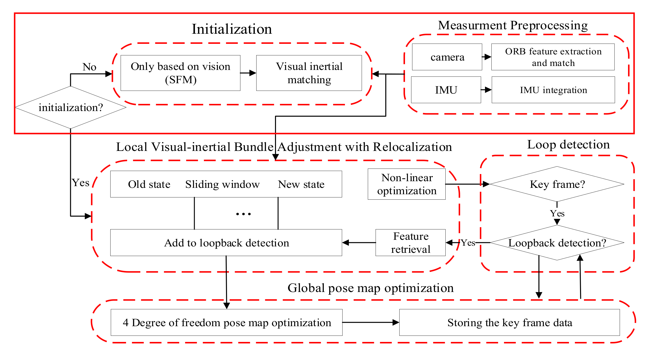
Both a monocular VINS and a visual SLAM essentially state estimation problems. Based on the VINS-mono project, this paper uses nonlinear optimization to couple IMU and camera data in a tightly coupled manner. The functional modules of the improved VINS-mono consist of five parts: data preprocessing, initialization, back-end nonlinear optimization, closed-loop detection, and closed-loop optimization. The code mainly opens four threads, including front-end image matching, back-end nonlinear optimization, closed-loop detection, and closed-loop optimization. The overall frame of the improved VINS-mono system is shown in Figure 1, where the red solid line represents the improvement parts compared with the VINS-mono. The main functions of each functional module are as follows.

Figure 1. The improved visual-inertial navigation system (VINS)-mono system architecture framework.

(1) Image and IMU preprocessing. The acquired image is processed with a pyramid presentation. The ORB feature points are extracted from each layer of the image. The adjacent frames are matched according to the feature points method. The outliers are removed by Random Sample Consensus (RANSAC) [31]. Finally, the tracking feature points are pushed into the image queue, and a notification is sent to the back end for processing. The IMU data are integrated to obtain the position, velocity, and rotation (PVQ) of the current time, and the pre-integration increments of the adjacent frames, the Jacobian matrix, and the covariance terms of the pre-integration errors used in the back-end optimization are calculated.

(2) Initialization. Structure From Motion (SFM) [32] is used for the pure visual estimation of the poses and 3D positions of all key frames in the sliding window. Then, the initial parameter calculation is performed by combining the IMU pre-integration results.

(3) Local visual-inertial bundle adjustment with relocalization. The visual constraints, IMU constraints, and closed-loop constraints are put into a large objective function for nonlinear optimization in order to solve the speed, position, attitude, and bias of all frames in the sliding window.

(4) Closed-loop detection and optimization. The Open-Source Library-Dictionary Bag-of-Words (DBoW3) is used for closed-loop detection. When the detection is successful, the relocation is performed, and finally the entire camera trajectory is closed-loop optimized.

3. The Initialization Process of the Improved VINS-Mono

VINS-mono does not initialize acceleration bias $b_a$ which simply sets its initial value to zero, which is not applicable to low-precision IMUs. The initialization result directly affects the robustness and positioning accuracy of the entire tightly coupled system.

In this paper, a new initialization scheme is designed, which can calculate the acceleration bias $b_a$ during the initialization process so that it can be applied to low-cost IMU sensors. Besides, the ORB feature point method is used instead of optical flow method to make the initialization model more accurate and robust during the initialization process.

The VINS-mono visual processing uses the optical flow tracking method. The accuracy of the pose solved by the optical flow tracking is not as good as the feature point matching, which has a great influence on the accuracy of the initialization and is directly related to the accuracy of the subsequent motion estimation. In order to improve this situation, in this paper, the ORB feature point method is used for pose estimation in the initialization phase. The flow of the initialization is shown in Figure 2.

Figure 2. Procedure of initializing of the improved VINS-mono.

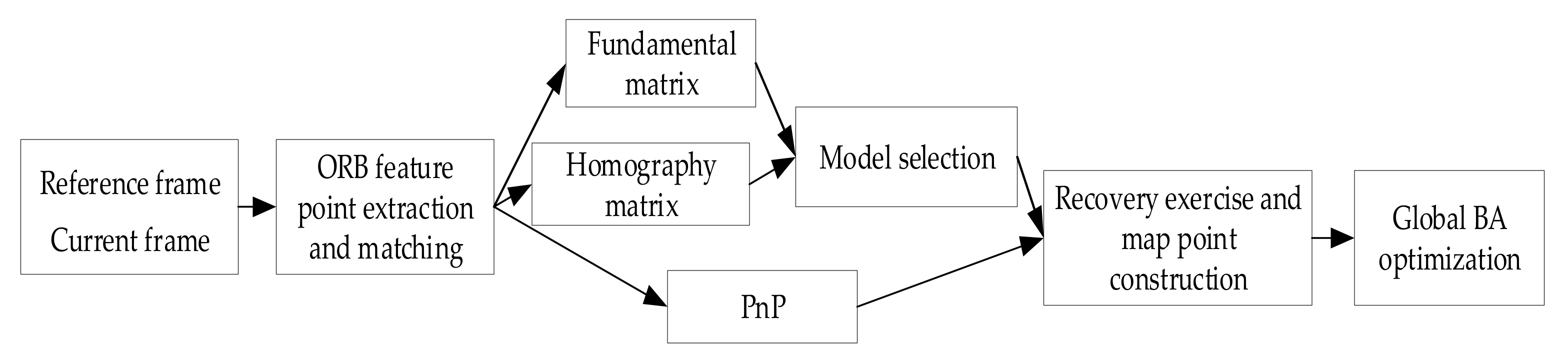
3.1. Visual SFM

The visual initialization uses the key frames image sequences in the initial time about 10 s to perform the pose calculation and triangulation as well as further global optimization. The selection of the image key frame is mainly based on the distance of the parallax, and when the parallax distance is greater than a certain threshold, it is selected as a key frame. The vision based SFM technique is used to obtain the more accurate pose and image point coordinates of the key frame sequence. This provides more accurate pose parameters for IMU initialization. In order to make the visual initialization independent of the scene, that is, to determine whether the initial scene is flat or non-planar, a relatively accurate initial value can be obtained. The two initial key frames images of the system adopt a parallel computing fundamental matrix and a homography matrix method and choose the right model according to a specific mechanism. The scene scale is fixed, and the triangle points are initialized according to the initial two key frames, then the Perspective-n-Point (PnP) algorithm is used to restore motion and continuously triangulate to restore the map point coordinates. After tracking a sequence, a Bundle Adjustment (BA) is constructed based on the projection error of the image coordinates for global optimization, and the optimized map points and poses are obtained, as shown in Figure 3.

Figure 3. Visual Structure from Motion (SFM) flowchart.

3.1.1. Two Parallel Computing Models and Model Selection

During the movement of the camera, the visual initialization may occur for the case of pure rotation or the distribution of feature points on the same plane. In this case, the degree of freedom of the fundamental matrix is degraded, and a unique solution cannot be obtained. Therefore, in order to make the initialization more robust, two models of parallel computing for the fundamental matrix and homography matrix are adopted. Finally, a model is chosen with a lower re-projection error, and the motion and map construction resume.

In practice, there are a large number of mismatches in feature matching. Using these points directly is inaccurate for solving the fundamental matrix and the homography matrix. Therefore, the RANSAC algorithm is used in the system to remove the mismatched pairs. Then, using the remaining pairs of points to solve the fundamental matrix and the homography matrix, the pose transformation under different models is further derived. Since the monocular vision has scale uncertainty, the scale needs to be normalized in the decomposition process. The initial map points can then be further triangulated by the two models.

Finally, the pose parameters recovered by the two models are used to calculate the re-projection error, and the model with a lower re-projection error is selected for motion recovery and map construction.

3.1.2. BA Optimization

In the system, after the visual initialization, there are already triangular map points, and the pose of remaining key frames can be solved with 3D-2D. In order to prevent the degradation of the map points in this process, it is necessary to continuously triangulate the map points and finally construct a Bundle Adjustment (BA) based on the key frame data. The position and pose of the camera and the coordinates of the map points are optimized, and the objective function of the optimization is as follows:

$$J(x)={\sum }_{j=1}^N{\sum }_{i=1}^{N_j}{e}_i^{j^T}W e_i^j.$$

(1)

In the formula, $N$ represents the number of key frames, $N_j$ represents the number of map points visible in each frame, $e$ represents the re-projection error of the pixel coordinates, and $W$ represents the weight matrix.

3.2. Visual-inertial Alignment

The purpose of visual-inertial alignment is to use the results of the visual SFM to decouple the IMU and calculate its initial values separately. The initialization process can be decomposed into four small problems in order to solve:

(1)

Estimation of the gyroscope bias

(2)

Estimation of the scale and the gravitational acceleration

(3)

Estimation of the acceleration bias and the optimization of the scale and gravity

(4)

Speed estimation

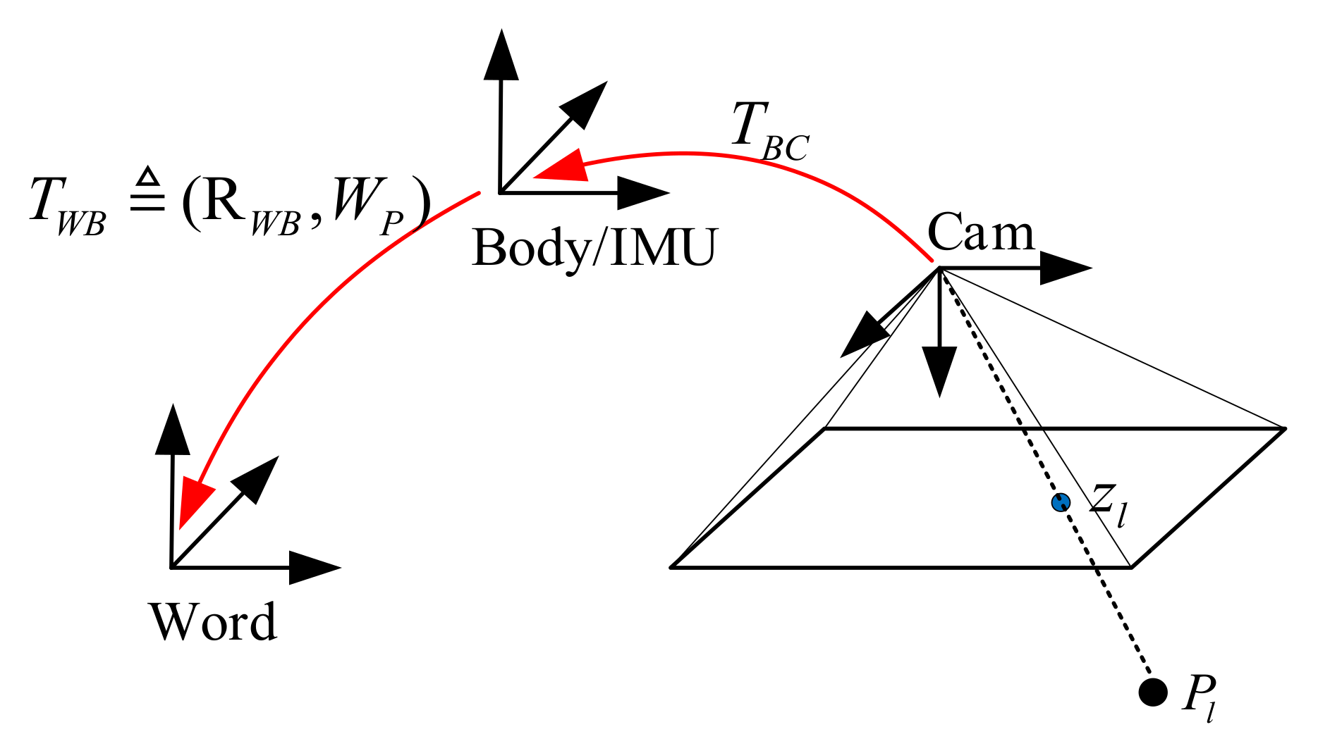
In order to describe the movement of the rigid body in three-dimensional space and the positional relationship between the camera and the IMU sensor mounted on the rigid body, the positional transformation relationship is defined as shown in Figure 4. The IMU coordinate system and the rigid body coordinate system (body) are defined as coinciding. $T_{BC}$ represents the transformation of the coordinates in the camera coordinates to the IMU coordinate system, and it is composed of $R_{BC}$ and $t_{BC}$. $T_{WB}$ denotes the transformation relationship between the rigid body coordinate system and the world coordinate system ($R_{WB}$ denotes the rotating part, and $W_P$ denotes the translation part). $P_l$ and $z_l$ represent world coordinates and image plane coordinates, respectively.

Figure 4. Conversion relations of different coordinate systems.

3.2.1. Gyro Bias Estimation

The bias of the gyroscope can be decoupled from the result of the rotation calculated by the visual SFM and the result of the IMU pre-integration. During the initialization process, it can be assumed that $b_g$ is a constant and does not change over time. Throughout the initialization process, the rotation of the adjacent key frames can be solved by the visual SFM. The rotation between adjacent frames can also be obtained by the pre-integration of the IMU. Assuming that the rotation matrix obtained by visual SFM is accurate, the value of $b_g$ can be calculated indirectly using the difference between the two rotation matrices corresponding to Lie algebra. The exponential map (at the identity) Exp: so(3)→SO(3) associates an element of the Lie Algebra to a rotation and coincides with the standard matrix exponential (Rodrigues’ formula).

The calculation formula is as follows:

$$\underset{b_g}{\mathrm{argmin}}{\sum }_{i=1}^{n-1}\parallel \mathrm{Log}{\left({(R_{BW}^{i+1}{R}_{WB}^i)}^T{\mathsf{\Delta }R}_{i,i+1}\mathrm{Exp}\left(J_{\mathsf{\Delta }R}^g{b}_g\right)\right)\parallel }^2$$

(2)

where the Jacobians $J_{\Delta R}^g$ account for a first-order approximation of the effect of changing the gyroscope biases without explicitly recomputing the pre-integrations. Both pre-integrations and Jacobians can be efficiently computed iteratively as IMU measurements arrive [28]. The above formula $R_{WB}^{(\cdot )}=R_{WC}^{(\cdot )}{R}_{CB}$, $n$ represents the number of key frames, and $\Delta R_{i,i+1}$ represents the integral value of the gyroscope between two adjacent key frames. The superscript $i$ represents the time of the key frame. $R_{WC}^{(\cdot )}$ can be obtained with visual SFM, and $R_{CB}$ is the rotation matrix of the IMU coordinate system in the camera coordinate system. Formula (2) can be solved with the Levenberg–Marquard algorithm based on nonlinear optimization, which is more robust than the Gauss–Newton method, and the value of $b_g$ can be decoupled.

3.2.2. Scale and Gravity Estimation

$b_g$ is calculated, brought into the pre-integration formula again, and then the position, speed, and rotation between adjacent frames are recalculated. Because the position calculated by visual SFM does not have real scale, the conversion between the camera coordinate system and the IMU coordinate system includes a scale factor s. The transformation equation of the two coordinate systems is as follows [26]:

$${}_{W}P_B=s{}_{W}P_C+R_{WC}{}_{C}P_B$$

(3)

It can be seen from the IMU pre-integration [28] that the motion between the two consecutive key frames can be written as follows:

$$\left\{\begin{array}{l}{R}_{WB}^{i+1}=R_{WB}^i\Delta R_{i,j+1}Exp((J_{\Delta R}^g{b}_g^i))\\ {}_{W}v_B^{i+1}=R_{WB}^i(\Delta v_{i,j+1}+J_{\Delta v}^g{b}_g^i+J_{\Delta R}^a{b}_a^i)+{}_{W}v_B^i+g_w\Delta t_{i,j+1}\\ {}_{W}p_B^{i+1}=R_{WB}^i(\Delta p_{i,j+1}+J_{\Delta p}^g{b}_g^i+J_{\Delta p}^a{b}_a^i)+{}_{W}p_B^i+{}_{W}v_B^i\Delta t_{i,j+1}+\frac{1}{2}{g}_w\Delta t_{i,j+1}^2\end{array}\right.$$

(4)

In the formula, $W$ represents the world coordinate system, and $B$ represents the IMU coordinate system or carrier coordinate system.

The accelerometer bias is relatively small to the gravitational acceleration, and therefore can then be neglected. When Formula (4) is introduced in Formula (3), the following formula is obtained:

$$\begin{array}{c}{s}_W{p}_C^{i+1}=s_W{P}_C^i+{}_{w}v_B^j\Delta t_{i,j+1}+\frac{1}{2}{g}_w\Delta t_{i,j+1}^2\\ \hspace{1em}\hspace{1em}+R_{WB}^i\Delta P_{i,i+1}+(R_{WC}^i-R_{WC}^{i+1}){}_{C}p_B\end{array}$$

(5)

The purpose of this formula is to solve for the scale factor s and the gravity vector. It can be seen that the above equation contains velocity variables. To reduce the computation and to eliminate the velocity variables, the following transformations are performed. Formula (5) is a three-dimensional linear equation. The data of the three key frames can be used to list the two sets of linear equations, and the velocity variables can be eliminated by using the speed relationship of Formula (4). We can write Formula (5) as a vector form:

$$\left[\begin{array}{cc}\alpha \left(i\right)& \beta \left(i\right)\end{array}\right]\left[\begin{array}{c}s\\ g_w\end{array}\right]=\gamma \left(i\right)$$

(6)

To facilitate the description, three keyframe symbols, $i$, $i+1$, and $i+2$ are written as 4, 5, and 6. The specific forms are as follows:

$$\left\{\begin{array}{l}\alpha (i)=({}_{W}p_C^5-{}_{W}p_C^4)\Delta t_{56}-({}_{W}p_C^6-{}_{W}p_C^5)\Delta t_{56}\\ \beta (i)=\frac{1}{2}{I}_{3\times 3}(\Delta t_{45}^2\Delta t_{56}+\Delta t_{23}^2\Delta t_{45})\\ \gamma (i)=(R_{WC}^5-R_{WC}^4){}_{C}p_B\Delta t_{56}-(R_{WC}^6-R_{WC}^5){}_{C}p_B\Delta t_{45}\\ \hspace{1em}\hspace{1em}+R_{WB}^5\Delta p_{56}\Delta t_{45}+R_{WB}^4\Delta v_{45}\Delta t_{45}\Delta t_{56}\\ \hspace{1em}\hspace{1em}-R_{WB}^4\Delta p_{45}\Delta t_{56}\end{array}\right..$$

(7)

Formula (6) can be constructed as a linear system in the form of $A_{3(N-2)\times 4}{x}_{4\times 1}=B_{3(N-2)\times 1}$. The scale factor and the gravity vector form a four-dimensional variable, so at least four frames of key frame data are needed for a Singular Value Decomposition (SVD) [33] solution.

3.2.3. Estimation of the Acceleration Deviation and the Optimization of the Scale and Gravity

It can be seen from Formula (5) that the accelerometer bias is not considered in the process of solving for the gravity and the scale factor, because the biases of the acceleration and gravity are difficult to distinguish, but it is easy to form a pathological system without considering the bias of the accelerometer. In order to increase the observability of the system, some prior knowledge is introduced. It is known that the gravitational acceleration of the Earth $G$ is 9.8 $\mathrm{m}/{\mathrm{s}}^2$, and the direction points to the center of the earth. Under the inertial reference frame, the direction vector of gravity is considered to be ${\widehat{g}}_I=\left\{0,0,-1\right\}.$ According to $g_w^{*}$, the direction ${\widehat{g}}_W=g_w^{*}/‖g_w^{*}‖$ of gravity can be calculated, and the rotation matrix of the inertial coordinate system to the world coordinate system can be further calculated, as follows [26]:

$$\left\{\begin{array}{l}{R}_{WI}=Exp(\widehat{v}\theta )\\ \widehat{v}=\frac{{\widehat{g}}_I\times {\widehat{g}}_W}{‖{\widehat{g}}_I\times {\widehat{g}}_W‖}\\ \theta =\arctan (‖{\widehat{g}}_I\times {\widehat{g}}_W‖, {\widehat{g}}_I\cdot {\widehat{g}}_W)\end{array}\right.$$

(8)

So, the gravity vector can be written as:

$$g_W=R_{WI}{\widehat{g}}_{I}G.$$

(9)

The z-axis of the world coordinate system is aligned with the gravity direction, so $R_{WI}$ only needs to parameterize and optimize the angle around the x-axis and the y-axis. The perturbation is used to optimize the rotation as follows:

$$\left\{\begin{array}{l}{g}_W=R_{WI}Exp(\delta \theta ){\widehat{g}}_{I}G\\ \delta \theta ={\left[\begin{array}{cc}\delta {\theta }_{xy}^T& 0\end{array}\right]}^T\\ \delta {\theta }_{xy}^T={\left[\begin{array}{cc}\delta {\theta }_x& \delta {\theta }_y\end{array}\right]}^T\end{array}\right.$$

(10)

The first-order approximation of Formula (10) is obtained as follows:

$$g_W\approx R_{WI}{\widehat{g}}_{I}G-R_{WI}{({\widehat{g}}_I)}_{\times }G\delta \theta$$

(11)

Formula (11) is introduced into Formula (3), then the bias of acceleration is taken into consideration, and the following formula is obtained:

$$\begin{array}{l}{s}_W{p}_C^{i+1}=s_W{p}_C^i+{}_{W}v_B^i\Delta t_{i,i+1}-\frac{1}{2}{R}_{WI}({\widehat{g}}_I){}_{\times }G\Delta t_{i,i+1}^2\delta \theta \\ \hspace{1em}\hspace{1em}\hspace{1em}+R_{WB}^i(\Delta p_{i,i+1}+J_{\Delta p}^{\alpha }{b}_a)+(R_{WC}^i-R_{WC}^{i+1}){}_{C}p_B\\ \hspace{1em}\hspace{1em}\hspace{1em}+\frac{1}{2}{R}_{WI}{\widehat{g}}_{I}G\Delta t_{i,i+1}^2.\end{array}$$

(12)

Similar to Formula (6), in three consecutive key frames, speed variables can be eliminated, and the following forms can be obtained:

$$\left[\begin{array}{ccc}\lambda (i)& \varphi (i)& \varsigma (i)\end{array}\right]\left[\begin{array}{c}s\\ \delta {\theta }_{xy}\\ b_a\end{array}\right]=\psi (i)$$

(13)

$\lambda (i)$ is the same as Formula (6). $\varphi (i)$, $\varsigma (i)$, and $\psi (i)$ are written as follows:

$$\left\{\begin{array}{l}\varphi (i)={\left[\frac{1}{2}{R}_{WI}{({\widehat{g}}_I)}_{\times }G(\Delta t_{45}^2\Delta t_{56}+\Delta t_{56}^2\Delta t_{45})\right]}_{(:,1:2)}\\ \varsigma (i)=R{c}_{WB}^2{J}_{\Delta p_{56}}^a\Delta t_{45}+R_{WB}^1{J}_{\Delta v_{56}}^a\Delta t_{45}\Delta t_{56}\\ \hspace{1em}\hspace{1em}-R_{WB}^1{J}_{\Delta p_{45}}^a\Delta t_{56}\\ \psi (i)=(R_{WB}^2-R_{WB}^1){}_{C}p_B\Delta t_{56}-(R_{WB}^3-R_{WB}^2){}_{C}p_B\Delta t_{45}\\ \hspace{1em}\hspace{1em}+R_{WB}^2\Delta P_{56}\Delta t_{45}+R_{WB}^1\Delta v_{45}\Delta t_{45}\Delta t_{56}\\ \hspace{1em}\hspace{1em}-R_{WB}^1\Delta P_{45}\Delta t_{56}+\frac{1}{2}{R}_{WI}{\widehat{g}}_{I}G\Delta t_{i,j}^2\end{array}\right.$$

(14)

In formula (14), the $(:,1:2)$ represents the first two columns of the matrix. According to the relationship between the consecutive key frames, a similar form of the linear system $A_{3(N-2)\times 6}{x}_{6\times 1}=B_{3(N-2)\times 1}$ can be constructed according to Formula (13). This linear system has six variables and $3(N-2)$ equations, so at least four keyframe datasets are needed to solve the linear system. The ratio of the maximum singular value to the minimum singular value is obtained by SVD decomposition to verify whether the problem is well solved. If the ratio is less than a certain threshold, Formula (12) can be re-linearized to solve the problem iteratively.

According to the above subsections, $b_g$, $s$, $g_W$, and $b_a$ have been determined. So far, there are only $3\ast N$ variables related to velocity. At this time, the speed of each key frame can be calculated by substituting $b_g$, $s$, $g_W$, and $b_a$ into Formula (12).

4. Local Visual-Inertial Bundle Adjustment with Relocalization

After the initialization of the improved VINS-mono system, subsequent Local visual-inertial bundle adjustment with relocalization can be carried out. Besides, the visual matching positioning method based on feature point method switches to optical flow tracking visual positioning mode. Because the calculation of descriptors and the matching of feature points are omitted, compared with the feature point method, the optical flow method is less sensitive to the environment texture and saves more computing resources. This is the reason why we choose the optical flow method after the initialization process. The VINS-mono system elaborates the rest of the process, including the nonlinear optimization and the marginalization strategy of the sliding window, closed-loop detection and optimization, and global pose optimization, this paper does not expound upon it too much.

5. Experimental Results and Analysis

The experiment on the initialization of the improved VINS-mono system was based on EuRoC, the unveiled dataset used to make the accuracy analysis and verification. The Swiss Federal Institute of Technology (ETH Zurich) collected the data with a binocular VIO camera carried on a drone and completed the dataset for the mainstream dataset of the test of monocular VINS system. The dataset consisted of two scenes, namely an industrial workshop and an ordinary indoor scene, as shown in Figure 5, while the dataset was divided into three categories, easy, medium, and complex, according to the number of environment-featured textures, the change of light, the speed of motion, and the image quality. This experiment only adopted the acceleration and the acceleration information measured by the IMU and the sequence of images acquired by the left-eye camera. We also test our algorithm with an Intel i5-6500HQ CPU running at 2.60GHz in real-time in the experiments. Since the feature point method is just used in the initialization phase, the improved VINS-mono and VINS-mono have the same computational cost in the real-time localization phase.

Figure 5. Some figures describe EuRoC dataset scenario [34] (a) Room Scene 1 (b) Room Scene 2 (c) Industrial Workshop Scene 1 (d) Industrial Workshop Scene 2.

5.1. Initialization Experiment

In this study, tests were conducted on dataset at two difficulty levels in different scenes (MH_01_easy, V2_02_medium). The purpose of this experiment was to test the convergence of system variables in the initialization process. Figure 6 and Figure 7 show the curves for the accelerometer bias, the bias of the gyroscope, the scale, and the number of system variables during the initialization process, which have good agreement with the convergence of each variable in the process. It can be seen from Figure 6 and Figure 7 that within approximately 10 s, the bias of the accelerometer and the bias of the angular speedometer with the IMU converged to a stable value, while the scale estimate was close to the optimized value. The optimized value was obtained by a similarity transformation of the posture estimation and the true pose. After 10 s, the condition number dropped significantly, and the convergence occurred, indicating that the system has a faster convergence rate. Figure 6 and Figure 7 also shows the evolution in the condition number, indicating that some time is required to get a well-conditioned problem. This confirms that the sensor must perform a motion that makes all variables observable, especially the accelerometer bias. In other words, if each initial value were precisely estimated to ensure the observability, the system would be properly initialized. The proposed initialization allows to start fusing IMU information, as gravity, biases, scale and velocity are reliably estimated.

Figure 6. This figure describes the results of initialization of variables in dataset MH_01_easy dataset. (a,b) describe separately the result of gyroscope bias initialization and accelerometer bias. (c) describes the results of initialization of scale. (d) describes the convergence of the number of system variables.

Figure 7. This figure describes the results of initialization of variables in dataset V1_02_media dataset. (a,b) describe separately the result of gyroscope bias initialization and accelerometer bias. (c) describes the results of initialization of scale. (d) describes the convergence of the number of system variables.

In order to test the initialization ability more rigorously, we use the MH_01_easy dataset to evaluate the accelerometer bias at different times. In this dataset, the accelerometer bias is approximately [−0.0032, 0.026, 0.076] $\mathrm{m}/{\mathrm{s}}^2$ in x, y and z axes, respectively. In our algorithm, we maintain at least 15 frames for initial visual structure. In general, the first few seconds are used for initialization. We estimate accelerometer bias in the initialization phase. To verify the capability of initialization, we randomly select start times in the dataset. Figure 8 shows the accelerometer bias calibration performance in 20 tests with the different start times in MH_01_easy dataset. The three sub-figures are accelerometer bias in xyz axis, respectively. The average error of accelerometer bias in two dominant direction x and y are [8.01, 1.52] % respectively, if we define the accelerometer bias less than 10% is successful initialization, our initialization procedure performs 90% success rate in this dataset. In fact, the local visual-inertial bundle adjustment with relocalization can be successfully bootstrapped even the initial scale error is about 20%.

Figure 8. Accelerometer bias in the initialization procedure in MH_01_easy dataset. The figure contains the results in 20 tests with different start time.

To test whether the new initialization algorithm was adaptable to low-cost sensors, a standard MYNT binocular camera was used to test the initialization. The information fusion between the camera and the IMU sensor required the relationship $T_{bc}$ of their coordinate systems. The camera-IMU offline calibration was performed through the Kalibr toolbox [35] before initialization, and the two sensors were considered to be relatively fixed in subsequent calculations. In other words, the result about $T_{bc}$ solved by Kalibr toolbox were not changed during the testing of the campus environment. Besides, the other calibrations could be obtained by Kalibr toolbox, such as gyroscope bias, accelerometer bias, camera internal parameters, and so on, as shown in Table 3. During the experiment, the initialization of the improved VINS-mono was applied to the low-cost IMU sensors, which can initialize and locate efficiently. By comparing the results of calibrated by Kalibr toolbox with the results tested by initialization scheme proposed in this paper, Table 4 shows they are basically consistent. The trajectory of the experiment can be seen in Figure 9.

Table 3. The parameter of MYNT binocular camera calibrated by Kalibr toolbox.

	Parameter of MYNT Binocular Camera
Cam0	camera_model: pinhole intrinsics: [461.629, 460.152, 362.680, 246.049] distortion model: radtan distortion_coeffs: [−0.27695497, 0.06712482, 0.00087538, 0.00011556] T_cam_imu ($T_{bc}$): - [0.01779316, 0.99967548, −0.01822937, 0.07008564] - [−0.9998015, 0.01795238, 0.00860716, −0.01771024] - [0.00893159, 0.01807261, 0.99979679, 0.00399247] - [0.0, 0.0, 0.0, 1.0] timeshift_cam_imu: −8.121e-05s rostopic: /cam0/image_raw resolution: [752, 480]
Accelerometer	Accelerometer_noise_density: 1.88e-03 #Noise density (continuous-time)
	accelerometer_random_walk: 4.33e-04 #Bias random walk
Gyroscope	gyroscope_noise_density: 1.87e-04 #Noise density (continuous-time)
	gyroscope_random_walk: 2.66e-05 #Bias random walk

Table 4. Initialization result calibrated by using Kalibr toolbox and calculated by the initialization method.

	Calibration by Kalibr Toolbox	Calculation by the Initialization Method
Accelerometer bias ($\mathrm{m}/{\mathrm{s}}^2$)	4.33e-04	4.30e-04 1 4.51e-04 2
Gyroscope bias (rad/s)	2.66e-05	2.62e-05 1 2.75e-05 2

¹ represents the calculated acceleration bias of accelerometer and gyroscope in dormitory building. ² represents the calculated acceleration bias of accelerometer and gyroscope on the playground.

Figure 9. This figure describes the results of the initialization experiments carried out in indoor and outdoor environments. (a,b) describe separately the running trajectory of dormitory building and playground. Red dots represent the sparse point cloud formed by triangulation and the yellow line represents the running trajectory.

It was concluded that the new initialization method was a good solution for effectively initializing the variables of the VINS system consisted of low-cost sensors. As indicated in Figure 6 and Figure 7, this initialization algorithm could be used to complete the entire initialization process within approximately 10 s.

5.2. The State Estimation Experiment

The dataset adopted in state estimation experiment was the same as that in the IMU initialization experiment (MH_01_easy, V2_02_medium), and the improved VINS-mono system was tested with various difficulty levels and environments. In this research, the accuracy analysis was carried out on the tracks generated by different datasets, and then a further comparison with well-performed VINS-mono was conducted. From the accuracy comparison between the two systems, it is clear that the improved VINS-mono system had significant improvement.

In this experiment, the motion track of the carriers was obtained using the adoption of a dataset in two different test environments, as indicated in Figure 10. Since the dataset contained the real track coordinates, the accuracy of the track in the modified system could be worked out by the calculation of an error between the estimated trajectory and the real trajectory. According to Figure 11, the trajectory result error was small, and the cumulative error was properly eliminated when MH_01_easy data were running in the system. This was because the speed of collecting data for MH_01_easy with the drone was slow enough for the system to detect in a closed loop and hence to make a holistic optimization. After the testing of the results of the improved VINS system in two different environments, the trajectory accuracy of the improved monocular VINS-mono system was also tested in the rest of the EuRoc datasets, as shown in Table 5.

Figure 10. Improved VINS-mono Running results of the system in dataset MH_01_easy (a) and dataset V2_02_medium (b) (red line represents real trajectory, green line represents estimate trajectory).

Figure 11. The graph describes the trajectory error change of the improved system over time in dataset MH_01_easy (a) and Dataset V2_02_medium (b) testing.

Table 5. Trajectory accuracy of the improved VINS-mono (EuRoc Dataset).

EuRoc Dataset	Improved VINS-mono RMES (m)	Scale Error (%)
V1_01_easy	0.068	0.079
V1_02_medium	0.099	0.118
V1_03_difficult	0.130	0.128
V2_01_easy	0.067	0.112
V2_02_medium	0.073	0.108
V2_03_difficult	0.185	0.151
MH_01_easy	0.129	0.062
MH_02_easy	0.097	0.124
MH_03_medium	0.102	0.129
MH_04_diffeicut	0.143	0.104
MH_05_diffeicut	0.181	0.133

In order to accurately analyze the performance of the improved VINS-mono, in this paper, the accuracy of the improved VINS-mono is described in the form of a root mean square error (RMSE) [36]. The estimated pose of the key frame is expressed as $Q_i\in SE(3)$,$i=1\dots n$, and the true pose is expressed as $L_i\in SE(3)$ $i=1\dots n$. The S is corresponding to the least-squares solution that maps the estimated trajectory $Q_i$ onto the ground truth trajectory $L_i$. The root mean square error of all key frames was calculated to obtain the final trajectory accuracy results as follows:

$$F_i=L_i^{-1}S{Q}_i$$

(15)

$$RMSE(F_{1:n})={\left(\frac{1}{n}{\displaystyle \sum _{i=1}^n{‖trans(F_i)‖}^2}\right)}^{1/2}$$

(16)

According to Table 6, it can be seen that the improved VINS-mono system has less than 0.2 m test trajectory accuracy except for the V1_03_difficult sequences, because of the texture of the scene is too weak, the number of key points extracted is too small to match well. In addition, this paper also compares the accuracy of the improved VINS-mono and VINS-mono. According to Table 6 and Figure 12, the different data show that the improved VINS-mono system had better precision than the VINS-mono system.

Table 6. Accuracy comparison of improved VINS-mono system and VINS-mono system.

EuRoc DataSet	Improved VINS-Mono RMES (m)	VINS-Mono RMES (m)
OV1_01_easy	0.068	0.078
V1_02_medium	0.099	0.106
V1_03_difficult	0.130	0.135
V2_01_easy	0.067	0.089
V2_02_medium	0.073	0.090
V2_03_difficult	0.205	0.221
MH_01_easy	0.129	0.278
MH_02_easy	0.097	0.124
MH_03_medium	0.102	0.135
MH_04_diffeicut	0.143	0.239
MH_05_diffeicut	0.181	0.366

Figure 12. This figure describes error comparison analysis in dataset MH_01_easy. (a) Orientation error and (b) Translation error (red for VINS-mono system and blue for the improved VINS-mono system).

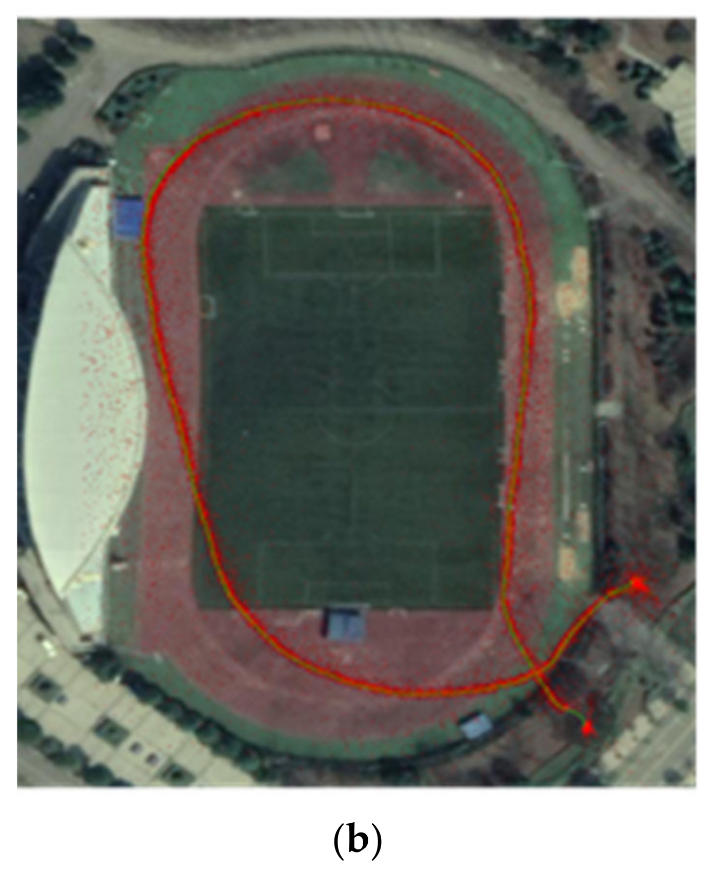
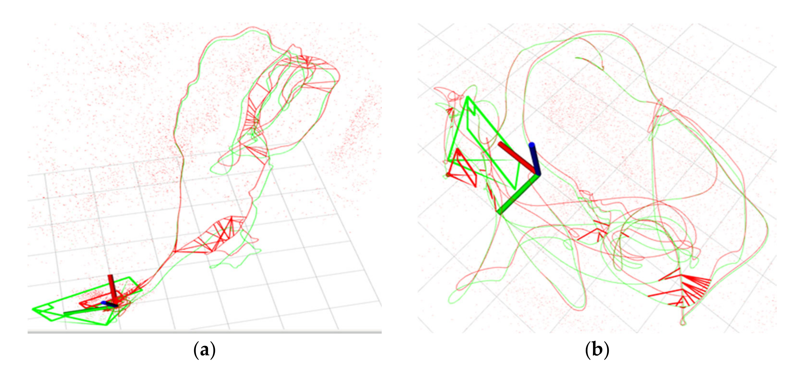
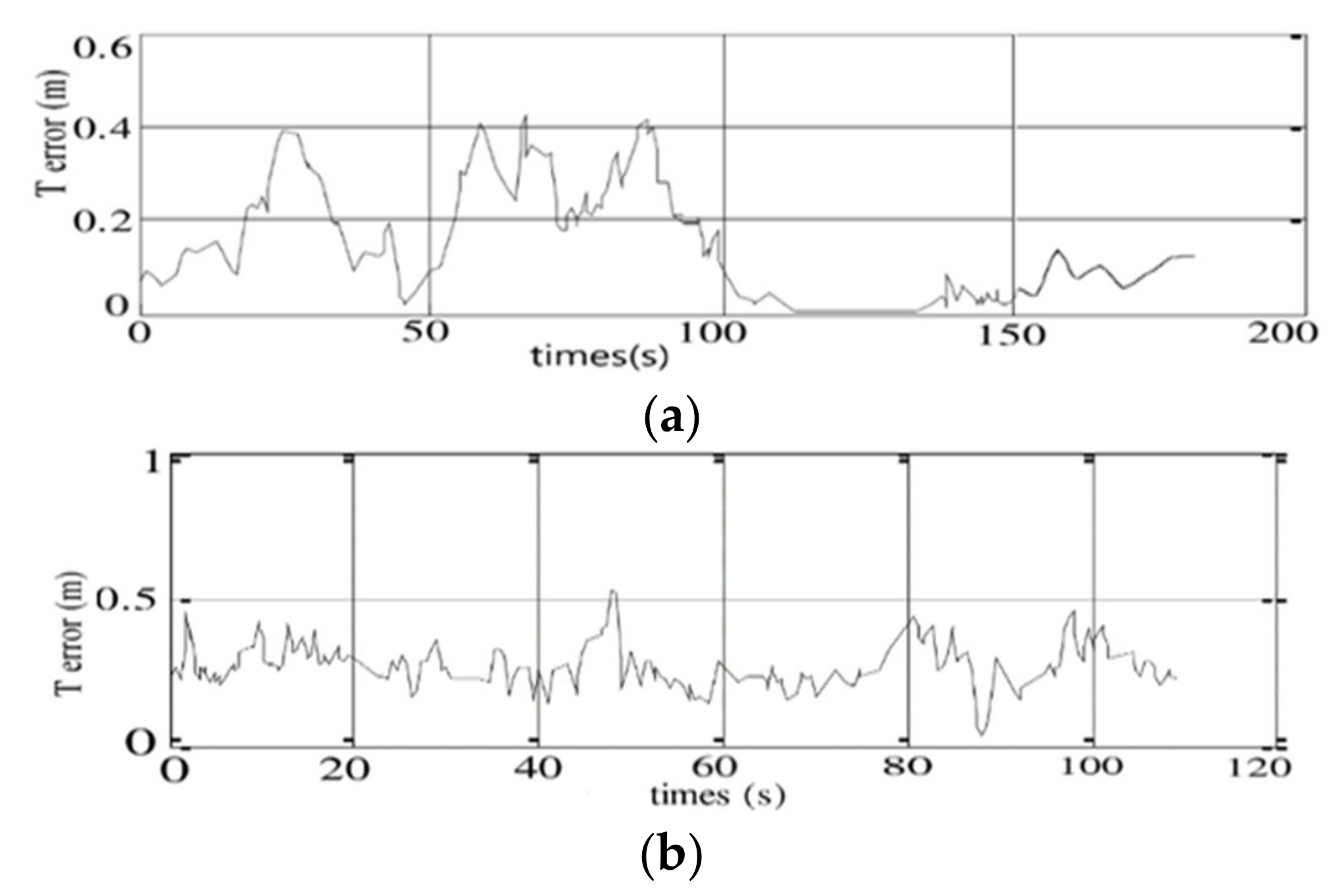
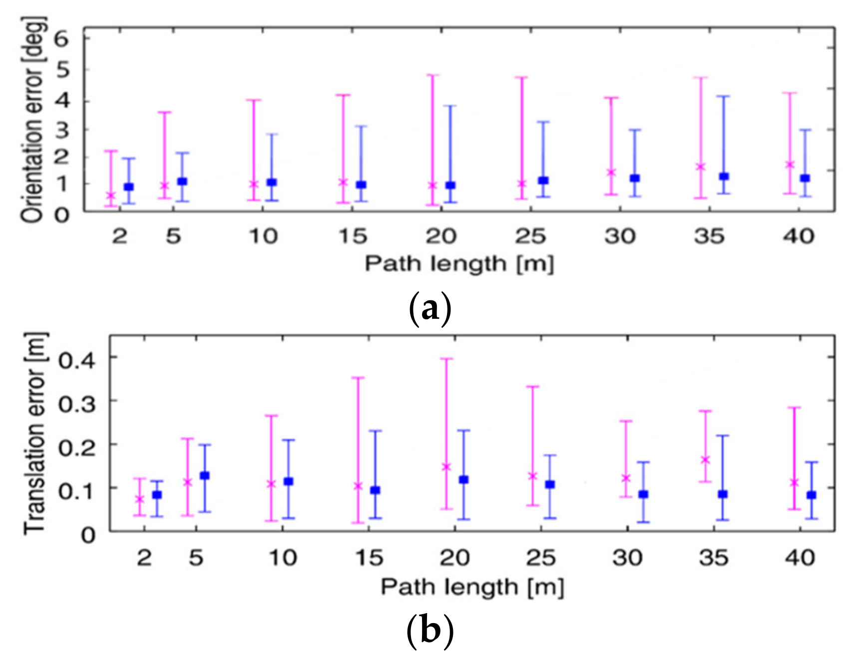
6. Conclusions

In this study, an initialization scheme was suggested to improve the accuracy and robustness of the visual-inertial navigation system. For this purpose, this paper designs a new initialization scheme which can calculate the acceleration bias as a variable during the initialization process so that it can be applied to low-cost IMU sensors. Besides, in order to obtain better initialization accuracy, a visual matching positioning method based on feature point method is used to assist the initialization process. After the initialization process, it switches to optical flow tracking visual positioning mode to reduce the calculation complexity. In the research, the improved VINS-mono was tested based on the unveiled dataset EuRoc and campus environment. The results show that the improved VINS-mono scheme completes the entire initialization process within approximately 10 s and can efficiently facilitate initialization with low-cost sensors. Due to the stricter initialization scheme to avoid the result from falling into the local minimum, the positioning accuracy is also improved.

The improved VINS-mono scheme still uses bag-of-word for loopback detection, but it can easily cause false results for loopback detection especially in an indoor environment that has many similar scenes. Therefore, further improvement of the robustness of the system loop detection is needed. Besides, this scheme can generate sparse point clouds information and it is necessary to generate dense 3D point clouds information of environment based on the video stream captured by camera real-time in the next work. In addition, it is necessary to fuse more sensor information to improve the positioning accuracy and robustness further in next step.