Article

Corn Biomass Estimation by Integrating Remote Sensing and Long-Term Observation Data Based on Machine Learning Techniques

1
Heihe Remote Sensing Experimental Research Station, Key Laboratory of Remote Sensing of Gansu Province, Northwest Institute of Eco-Environment and Resources, Chinese Academy of Sciences, Lanzhou 730000, China
2
Center for Excellence in Tibetan Plateau Earth Sciences, Chinese Academy of Sciences, Beijing 100101, China
3
Chongqing Jinfo Mountain Karst Ecosystem National Observation and Research Station, School of Geographical Sciences, Southwest University, Chongqing 400715, China
*
Author to whom correspondence should be addressed.
Remote Sens. 2021, 13(12), 2352; https://doi.org/10.3390/rs13122352
Submission received: 20 April 2021 / Revised: 7 May 2021 / Accepted: 10 June 2021 / Published: 16 June 2021
(This article belongs to the Special Issue Deep Learning Methods for Crop Monitoring and Crop Yield Prediction)

Abstract

:
The accurate and timely estimation of regional crop biomass at different growth stages is of great importance in guiding crop management decision making. The recent availability of long time series of remote sensing data offers opportunities for crop monitoring. In this paper, four machine learning models, namely random forest (RF), support vector machine (SVM), artificial neural network (ANN), and extreme gradient boosting (XGBoost) were adopted to estimate the seasonal corn biomass based on field observation data and moderate resolution imaging spectroradiometer (MODIS) reflectance data from 2012 to 2019 in the middle reaches of the Heihe River basin, China. Nine variables were selected with the forward feature selection approach from among twenty-seven variables potentially influencing corn biomass: soil-adjusted total vegetation index (SATVI), green ratio vegetation index (GRVI), Nadir_B7 (2105–2155 nm), Nadir_B6 (1628–1652 nm), land surface water index (LSWI), normalized difference vegetation index (NDVI), Nadir_B4 (545–565 nm), and Nadir_B3 (459–479 nm). The results indicated that the corn biomass was suitably estimated (the coefficient of determination (R2) was between 0.72 and 0.78) with the four machine learning models. The XGBoost model performed better than the other three models (R2 = 0.78, root mean squared error (RMSE) = 2.86 t/ha and mean absolute error (MAE) = 1.86 t/ha). Moreover, the RF model was an effective method (R2 = 0.77, RMSE = 2.91 t/ha and MAE = 1.91 t/ha), with a performance comparable to that of the XGBoost model. This study provides a reference for estimating crop biomass from MOD43A4 datasets. In addition, the research demonstrates the potential of machine learning techniques to achieve a relatively accurate estimation of daily corn biomass at a large scale.

1. Introduction

Crop biomass is one of the most important biophysical indicators of crop growth [1,2]. The accurate and efficient estimation of the regional crop biomass at different growth stages is of great importance in guiding crop management decision making, such as in effective fertilization, water irrigation, weeding, and pest and disease management [3,4]. In addition, as an important aspect of biomass energy, the accurate estimation of crop biomass contributes to the rational and effective utilization of biomass energy [5]. Moreover, effective estimates of crop biomass during the growing season could play a key role in crop yield prediction [6]. This is currently one of the major challenges for agricultural researchers and farm managers [7].
The traditional crop biomass estimation method is mainly based on field measurements, which include destructive field sampling, laboratory drying and weighting. The traditional methods are relatively accurate, but they are labor intensive and time consuming. Moreover, the sparse nature of space makes it impossible to provide a comprehensive understanding at regional or larger scales [2,8,9,10]. Thus, it is impossible to acquire the regional crop biomass via ground measurements alone. The satellite remote sensing technique is a unique and useful method for crop biomass monitoring in a repeatable manner due to the valuable information it provides on vegetation parameters, high spatial coverage and long time series, which effectively compensates for the deficiency of traditional biomass estimation methods [2,8,11,12,13]. Previous studies have revealed that remote sensing is a reliable and effective technique to obtain biophysical and biochemical crop information [6,14,15,16,17]. For example, the moderate resolution imaging spectroradiometer (MODIS) of the Earth Observation System (EOS) instrument provides long time series observations at a spatial resolution ranging from 250 to 1000 m in multiple spectral bands at the visible to shortwave infrared (SWIR) wavelengths, with a global coverage of one to two days, which has been widely applied in studies on the variation in vegetation parameters at the regional and global scales [18,19,20].
Various methods have been developed for crop biomass estimation based on optical remote sensing data, such as statistical, process-based, machine learning, and other methods [21]. Machine learning techniques have become a basic and effective way to model and extract patterns from remote sensing data due to their high computational efficiency, few required variables, and reliable results [14,21,22,23]. Machine learning techniques, including artificial neural networks (ANNs) [24], random forests (RFs) [25,26,27], support vector machines (SVMs) [28,29], and extreme gradient boosting (XGBoost) [30,31,32] have been widely implemented to evaluate vegetation biomass based on spectral signature parameters [1,17,33,34]. Although great progress has been attained in improving the spatially explicit estimation of crop biomass with machine learning methods based on multisource data, regional crop biomass estimates still exhibit large uncertainties at local scales [6,21,35]. There are several sources of uncertainty in crop biomass estimation. The first limitation is the lack of adequate field observation data, which may easily lead to the model becoming overfitted and failing to capture local features. The second limitation is that there is a need for the further comparison of available techniques, particularly machine learning techniques, for crop biomass estimation. Comparisons of these machine learning techniques have shown that each has its own advantages and drawbacks [11,17,22,30,33]. The third uncertainty originates from the input variable selection process according to the remote sensing data during the simulation process. Crop biomass was highly correlated with spectral signature parameters derived from satellite imagery, such as vegetation indices, which were calculated from different integrations of visible and NIR reflectance, leaf area, and reflectance for certain bands [1,6,10,11,17]. The input variable selection was based on its sensitivity to vegetation biomass. The input variables varied between studies, which made it difficult to analyze the uncertainty of the estimation biomass for machine learning models.
In this study, the corn biomass was estimated based on daily MODIS datasets with a 500 m spatial resolution combined with long-term ground observation data in the middle reaches of the Heihe River Basin, and four machine learning algorithms, namely RF, SVM, ANN, and XGBoost, were adopted to predict the biomass. The objectives of this study were (1) to validate the potential of MOD43A4 datasets with regard to corn biomass estimation; (2) to compare the performance of the RF, SVM, ANN, and XGBoost models in the estimation of corn biomass and examine suitable models; and (3) to generate an optimized framework for MODIS-based corn biomass estimation with high accuracy.

2. Materials and Methods

In this study, we selected the middle area of the Heihe River basin as the research area to carry out corn biomass estimation based on machine learning models. Figure 1 shows a schematic diagram of the steps and processes followed in the research. Overall, there are four major components: data and variable preparation, model parameter optimization, model performance assessment and comparison, and model application based on MODIS data at the country level. The following is a detailed description of each component.

2.1. Study Sites

The study area is situated in the middle reaches of the Heihe River basin, Gansu Province, China (Figure 2). The Heihe River basin, located in the middle of the Hexi Corridor, is the second largest inland river basin in China. It consists of three regions: the upper mountain zone, middle oasis zone and lower arid zone. The middle reaches of the Heihe River basin cover an area of approximately 8700 km2 and are an important food base in Northwest China. The climate is continental, with an annual average temperature of 7.5 °C [36]. The annual rainfall ranges from 100 to 250 mm [37], and the annual potential evaporation reaches 1200–1800 mm [38]. Seed corn is the most important commercial crop in the middle reaches of the Heihe River. With the increase in seed corn sowing area, the study area has become an important seed corn-producing area in China [36]. It has been identified as the national seed corn production base since 2013.

2.2. Field Data

Large, relatively homogeneous areas, which mainly functioned as corn growing areas, were selected as the sample sites. According to a field survey of the sample sites, a total of sixteen sites were selected in 2012, and three sites were selected for field measurement purposes every year from 2013 to 2019. One to three plots for each sample site were chosen for further biomass observation, with each plot covering an area of 100 m × 100 m. The number of plots for each sample site was determined by the planting structure of corn at the site. For each plot, three corn plants representing the level of the plot were randomly selected. All selected plants in each plot were collected, and the roots of the corn plants were washed. The fresh weight was measured, after which the plants were transported to the laboratory, chopped into easy-to-dry segments, and dried in an oven at 85 °C for 48–72 h until a constant dry biomass was obtained. The average biomass value of the plots was considered to represent the biomass at the site scale. In situ biomass measurements were implemented from 2012 to 2019 during the growing season of corn. The observations occurred from mid-May to late September each year, i.e., from the beginning of corn growth to corn harvest, over a five-day period during the rapid growth period (before August) and over a ten-day period for days thereafter. The beginning observation date differed each year because the corn sowing time continuously changed in the study area. The number of corn plants per unit area was calculated by combining various structural parameters of corn planting, such as the plant spacing, row spacing and uplift spacing.

2.3. Remote Sensing Data and Processing

MODIS MCD43A4 and MOD15A2 products from May to September from 2012 to 2019 were analyzed in this study. MCD43A4 provides daily 500-m reflectance data adjusted via the nadir bidirectional reflectance distribution function-adjusted reflectance retrieved from combined MODIS-Terra and MODIS-Aqua acquisitions. Since the product removes land surface reflectance anisotropy and provides similar observations to those of the nadir view angle, it is a more stable and consistent product [39]. MCD43A4 has been adopted to monitor vegetation biomass and land surface disturbance due to its improved accuracy of change detection in intra- and interannual temporal dynamics [2,40]. MOD15A2 provides 8-day composite 1 km resolution leaf area index (LAI) data from Terra. The MODIS reprojection tool (MRT) was employed to reproject and resample MODIS images.

2.4. Land Cover Data

The land cover map of the Heihe River Basin of August 2015 was used in this study to generate a corn map of the study area [41,42,43] (Figure 2). Previous studies have demonstrated that the main planting area in the study area is seed corn [36,44,45], and the crop of seed corn is more than three times that of field corn [44]. It is difficult to distinguish seed and field corn planting areas in land cover data. Therefore, we considered both field corn and seed corn as corn in this study.

2.5. Model Variables and Optimization

Twenty-seven variables, including the LAI derived from the MODIS MOD15A2 product, seven MCD43A4 bands (Table 1), and nineteen spectral vegetation indices (Table 2) based on the visible and near-infrared (NIR) bands of MCD43A4 related to the vegetation biomass were adopted in this study. We selected those variables based on their sensitivity to the vegetation structure and biomass according to previous studies [1,3,6,31,34,40]. For example, the normalized difference vegetation index (NDVI), normalized difference water index (NDWI), enhanced vegetation index (EVI), and soil-adjusted vegetation index (SAVI) have been successfully used for biomass accumulation research because they are strongly correlated with vegetation biophysical parameters [40]. The LAI was sensitive for crop biomass estimation [1]. Furthermore, additional indices that were modified based on the NDVI with different integrations of visible and NIR reflectance were used, such as the green normalized difference vegetation index (GNDVI), blue normalized difference vegetation index (BNDVI), and wide dynamic range vegetation index (WDRVI). Additionally, the band of visible and NIR reflectance, which are relatively sensitive to vegetation biomass, were frequently used in biomass studies [26,31]. The forward feature selection method was implemented to choose the most influential variables, which is an iterative method starting from the condition of no model features. In each iteration, we add a given feature that best improves the model until the addition of a new variable does not further improve the model performance.

2.6. Machine Learning Algorithms

The RF, SVM, ANN, and XGBoost algorithms were adopted in this study. With regard to the RF algorithm, only two parameters are tuned: ntree and mtry. Parameter mtry is the number of splits per node in each tree during the building process, and ntree is the number of decision trees or the number of bootstrap samples [61]. The accuracy of the model is mainly influenced by the value of mtry [30,62]. Therefore, we set ntree as the default value of 500.
The SVM algorithm is largely based on the structural risk minimization principle and statistical theory [63,64]. The choice of the positive definite kernel function is very important in this method [62,65]. Moreover, with regard to the SVM algorithm, the cost factor and gamma affect the punishment imposed for sample misclassification and algorithm complexity [63]. In this study, the radial kernel function was chosen, and it includes the sigma and c parameters.
The ANN includes one input layer, one output layer and one or multiple hidden layers. Neural networks learn the relationship between the input and output variables via the establishment of a set of nonlinear units, which are organized into layers and connected by weights with deviations equivalent to those in the regression parameters of classical parametric models [11]. In this study, the Bayesian regularized neural network (BRNN) was employed, which is one type of ANN widely applied in prediction research [66]. The BRNN fits a two-layer neural network and uses the Nguyen and Widrow algorithm to assign initial weights and the Gauss–Newton algorithm to perform optimization. One parameter of the BRNN function is considered here, namely the number of neurons.
XGBoost performs a second-order Taylor expansion of the objective function and employs the second derivative to accelerate the model convergence speed during training [67]. In addition, a regularization term is added to the objective function to control the tree complexity, which generates a relatively simple model and prevents overfitting. The XGBoost algorithm contains many parameters, and the most important parameters in this study are: (1) max_depth, which is the maximum depth of an individual tree; (2) nrounds, which is the maximum number of iterations; (3) eta, which reduces the feature weights to ensure that the boosting process becomes more conservative; (4) gamma, which is the minimum loss reduction required to further partition a given leaf node of the tree; (5) subsample, which is the subsampling ratio of the training instances or rows; (6) colsample_bytree, which is the subsampling ratio of the columns during tree construction; (7) rate_drop, which is the fraction of previous trees to eliminate during the dropout procedure; (8) skip_drop, which is the probability of skipping the dropout procedure in a given boosting iteration; and (9) min_child_weight, which is the minimum sum of the instance weight needed in a leaf node. XGBoost model tuning is a complicated task because changing any one parameter affects the optimal values of the other parameters [30].
R software was used to implement the above four machine learning algorithms with the randomForest, kernlab, brnn, and xgboost packages. In this study, the caret package in R software was applied to tune the parameters of the above four machine learning algorithms. The caret package comprises a set of functions to streamline the process of creating prediction models. It contains tools for data splitting, preprocessing, feature selection, model tuning by resampling and variable importance estimation. The root mean squared error (RMSE), coefficient of determination (R2) and mean absolute error (MAE) were calculated during parameter tuning, and the minimum RMSE value was considered to select the optimal model. According to the optimal models determined in this study, the parameter mtry of the RF algorithm was set to 9, and sigma and C were set to 2.1 and 1, respectively, in the SVM algorithm, the number of neurons was set to 3 in the BRNN function of the ANN algorithm, and the max_depth, nrounds, eta, gamma, subsample, colsample_bytree, rate_drop, skip_drop, and min_child_weight parameters of the XGBoost algorithm were set to 3, 100, 0.4, 0, 1, 0.6, 0.5, 0.95, and 1, respectively.

2.7. Model Evaluation

The 10-fold cross validation method was implemented to evaluate the performance of the above four machine learning models due to the small number of training samples. According to the 10-fold cross validation method, the field observations were divided into 10 equal groups; nine groups were selected as training samples with which to build the corresponding regression model, and the remaining group was used as the validation sample to evaluate the trained model. R2 (Equation (1)), RMSE (Equation (2)), and MAE (Equation (3)) were determined to quantify the performance of the above four models. A high R2 value, low RMSE value and low MAE value indicate good model performance:
R 2 = 1 ( n 1 ) i = 1 n ( y ^ i y i ) 2 ( n 2 ) i = 1 n ( y ^ i y i ¯ ) 2
R M S E = 1 n i = 1 n ( y ^ i y i ) 2 )
M A E = 1 n i = 1 n | ( y ^ i y i |
where y ^ i   is the predicted biomass value, y i is the ground-measured biomass value, y i ¯   is the mean value of the ground-measured biomass, and n is the number of samples.

3. Results

3.1. Importance of Variable Optimization for Machine Learning Model Performance

The selection of suitable variables is a critical step in the development of a biomass estimation model because certain variables may be weakly correlated with the biomass, which may reduce the biomass estimation performance [35]. In this study, nine out of the twenty-seven variables were selected according to the forward feature selection method: SATVI, GRVI, Nadir_B7, Nadir_B6, LSWI, NDVI, Nadir_B4, Nadir_B3, and RVI. Figure 3 shows the relative correlation between the corn biomass and each of the nine optimal variables. The results indicated that all nine variables were significantly correlated with the corn biomass, and GRVI, LSWI, NDVI, and RVI were positively correlated with the biomass, while the remaining five variables were negatively correlated with the biomass. The correlation coefficients R of Nadir_B3, Nadir_B4, and NDVI were higher than 0.70, and the correlation coefficients R of the other variables were all above 0.60.

3.2. Model Performance and Accuracy Comparison

The performance of the four machine learning algorithms was further analyzed based on the nine optimal variables. The model performance was explained via scatter plots. Figure 4 shows the relationship between the observed and predicted biomass values. The results indicated that the XGBoost (R2 = 0.78, and RMSE = 2.86 t/ha) and RF (R2 = 0.77, and RMSE = 2.91 t/ha) models performed better than the SVM (R2 = 0.72, and RMSE = 3.20 t/ha) and ANN (R2 = 0.72, and RMSE = 3.20 t/ha) models with the same dataset, and the XGBoost model performed slightly better than the RF model because it attained the highest R2 and lowest RMSE values.
In addition, based on R2, MAE, and RMSE, as shown in Figure 5, we also found that the R2 values followed the order of XGBoost > RF > ANN > SVM, the RMSE values followed the sequence of XGBoost < RF < ANN < SVM, and the MAE values followed the order of XGBoost < RF < ANN < SVM, which indicated that the XGBoost model performed better than the other three models, followed by the RF model. Moreover, there was little difference in R2, MAE, and RMSE between the RF and XGBoost models. This verified that the RF model was also an effective model, with the XGBoost model performing slightly better than the RF model. The SVM performed worse than the other models in most situations.

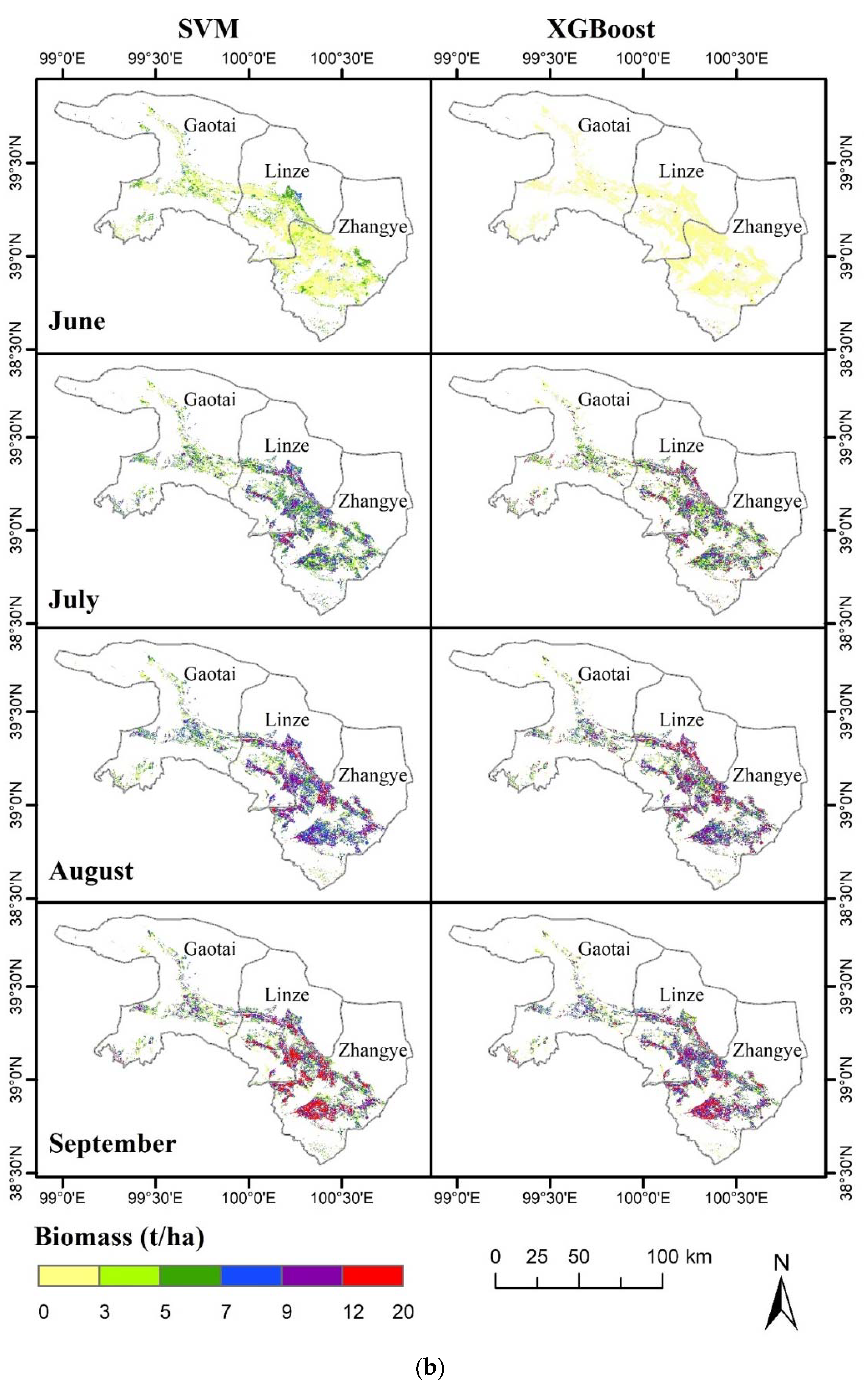
3.3. Visual Representation of the Spatiotemporal Characteristics of the MODIS-Estimated Biomass

To investigate the temporal performance of the RF, SVM, ANN and XGBoost models, a relatively homogeneous MCD43A4 pixel with long-term ground observation data was chosen to analyze the differences between the estimated and ground-observed biomass data. Figure 6 shows a temporal comparison of the ground-observed and estimated biomass data between the RF, SVM, ANN, and XGBoost models from 2012 to 2019. According to the visual assessment of the fitted time series curves (Figure 6), the estimated biomass trend curves of the four models were similar to the ground-observed biomass curves at most times. However, obvious differences were observed between the estimated and field-observed biomass values. Different degrees of biomass overestimation or underestimation occurred among the four models, especially after the tasseling stage, and the corn biomass suddenly decreased and then gradually increased (Figure 6a,e,g). The SVM model tended to overestimate the biomass during early corn growth (Figure 6c,d,f,h), while the data estimated with the other three models were very close to the observed data at this stage. It was difficult to distinguish the performance of the RF, ANN and XGBoost models based on the estimated data curves. In 2018, all four models tended to underestimate the corn biomass after mid-July (Figure 6g). The main reason is that the variety of corn in the observation area changed from seed corn to field corn, and the phenological periods of the two types of corn were significantly different. Unlike the field corn, seed corn is emasculated in mid-July, and then male-removed in early August. This is also the reason for the slower above ground biomass growth or sudden decrease in this period for most study years.
To examine the seasonal changes in the spatial distribution of the corn biomass, the biomass data estimated with the RF, SVM, ANN and XGBoost models in the study area were visualized. Figure 7 shows the seasonal differences in the spatial distribution of the four models based on the MCD43A4 data on the first day of June, July, August, and September 2019. Obvious differences occurred between the four models. For example, the estimated values of the SVM model in some regions in June were notably higher than those of the other three models, and the areas indicating a biomass between 3 and 5 t/ha of the SVM model were much larger than those of the RF, ANN, and XGBoost models. Moreover, the estimated values of the ANN model in certain regions in July and August were notably lower than those of the other three models, and the areas indicating a biomass between 9 and 12 t/ha of the ANN model were obviously smaller than those of the RF, SVM and XGBoost models.

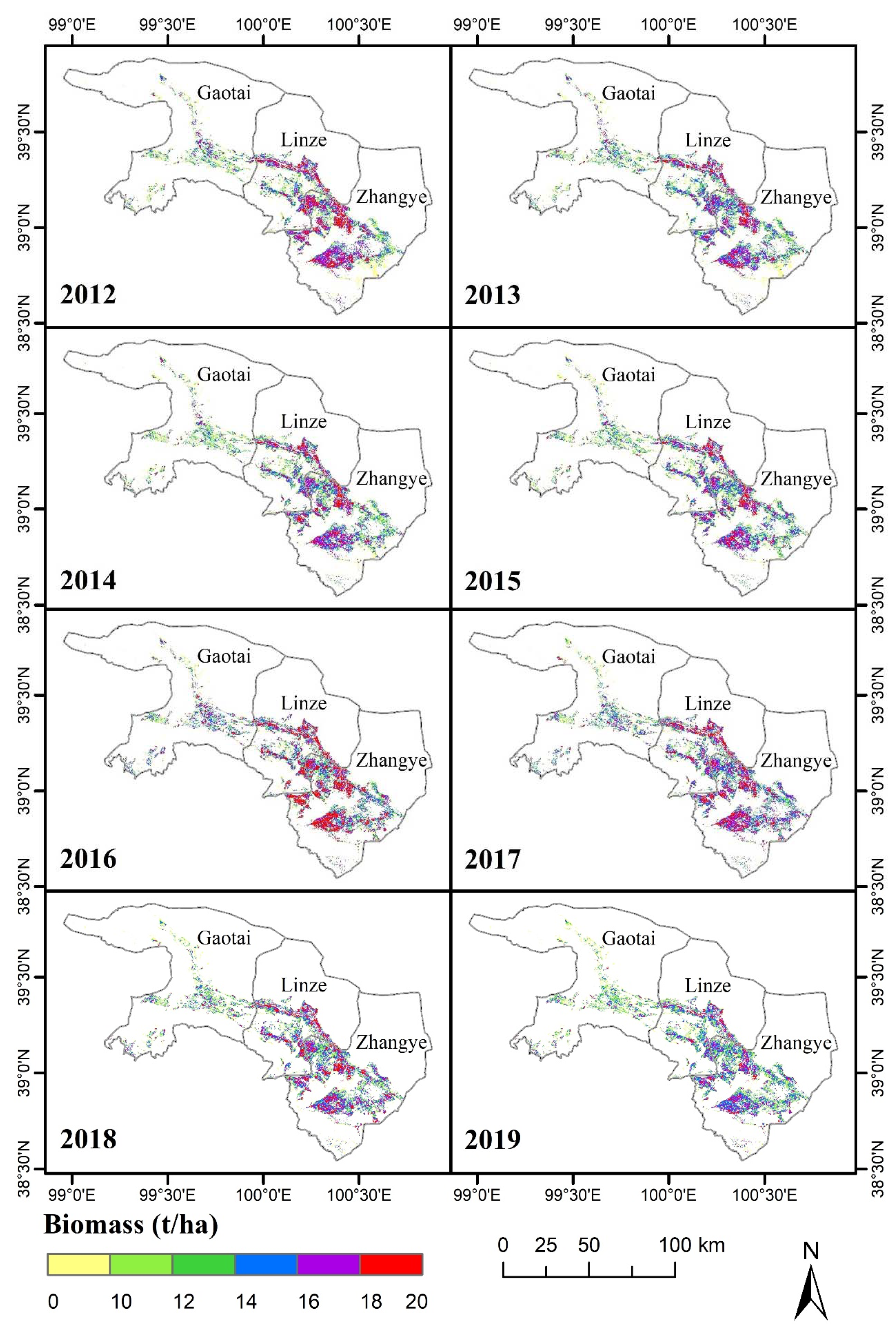
3.4. Spatial Distribution of the Simulated Biomass with the Highest-Performance Models

Based on the accuracy comparison of R2, RMSE, and MAE, the XGBoost and RF models were chosen as the two best performing models to carry out further spatial distribution analysis. Figure 8 shows the interannual differences in the spatial distribution of the simulated corn biomass obtained with the two best performing models based on the MCD43A4 data on the first day of August from 2012 to 2019. As shown in Figure 8, the XGBoost and RF models exhibited similar spatial distribution characteristics, and the corn biomass value was high in the southeast and moderate and low in the west. Moreover, it was found that the spatial distribution of the estimated biomass by the two models revealed similar interannual changes in certain years. For example, the areas indicating a biomass ranging from 5 to 7 t/ha and 7 to 9 t/ha in 2014 and 2015 were larger than those in the other years, while the areas indicating a biomass over 9 t/ha were much smaller in the same years for both models. However, there were differences in the areas of different predicted biomass ranges between the two models. The percentage of low- and high-biomass areas for the XGBoost model was higher than that for the RF model, while the percentages of moderate biomass areas for the RF model were higher than those for the XGBoost model during the study period. For example, the percentages of the areas indicating a biomass lower than 5 t/ha and over 12 t/ha for the XGBoost model were higher than those for the RF model, while the opposite was true for the areas indicating a biomass between 5 and 9 t/ha. Based on the best-performing model—XGBoost—we obtained the spatial characteristics of the annual variation in corn maximum biomass for the study area (Figure 9). Overall, the corn biomass was higher in the eastern and central parts than in the western part of the study area. The average biomass was 13.66–15.40 t/ha (the highest was in 2016, and the lowest was in 2013). The highest biomass (>16 t/ha) was concentrated in the central part of the study area where irrigation water resources are relatively abundant. The lowest biomass (<12 t/ha) was distributed in the western part of the study area.

4. Discussion

4.1. Importance of the Prediction Variables

Figure 10 shows the scatter plots of the ground-observed biomass and estimated biomass for the RF, SVM, ANN and XGBoost models based on all twenty-seven variables. Compared with Figure 4, it was found that the precision of the results after variable optimization was greatly improved for all four models. The R2 value for both the RF and XGBoost models was 0.75 before variable optimization but increased to 0.77 and 0.78, respectively, after variable optimization. In addition, RMSE decreased from 3.03 to 2.901 t/ha and from 3.00 to 2.86 t/ha for the RF and XGBoost models, respectively. Similarly, for the ANN and SVM models, R2 increased and RMSE decreased to different degrees.
Table 3 summarizes the variable selection results obtained with the forward feature selection method starting from the initial 27 variables, and Figure 11 shows the process of the forward feature selection method in this study. The best bivariate model includes SATVI and GRVI with mean R2 and RMSE values of 0.7266 and 3162.03 kg/ha, respectively. When Nadir_B4 and Nadir_B7 are added to the model, the R2 and RMSE values are 0.7392 and 3097.89 kg/ha, respectively. With the addition of the other five variables (LSWI, NDVI, Nadir_B6, Nadir_B3, and RVI), R2 slightly increases from 0.7527 to 0.7739, and RMSE decreases from 3011.75 to 2886.80 kg/ha.
The variable importance results in Table 3 show that the SATVI and GRVI play an important role in corn biomass estimation in this study, which is in stark contrast to other studies because SATVI has not been as widely adopted as other vegetation indices. However, SATVI, as an index of the amount of green and senescent vegetation, is highly correlated with vegetation coverage [52,68]. SATVI can capture 55% of the variability in ground measured total vegetation cover from diverse sites [69], and it has been utilized to analyze that of fractional plant cover changes [68]. There was a strong correlation between corn biomass and coverage, and it is a reasonable key variable in this study. GRVI showed great sensitivity to nitrogen deficiency in corn, and previous studies have shown a higher correlation with corn yield [70,71]. LSWI is a vegetation water content index, which is also a key variable for this research. This finding is consistent with the results reported by Wang et al., who indicated that LSWI had a better relationship with biomass than NDVI and EVI [72]. The RVI and NDVI play crucial roles in the dry matter of vegetation [73,74], and they have been demonstrated to be strongly correlated with vegetation biomass in previous studies [75,76,77]. In this study, the four MCD43A4 reflectance wavebands, namely SWIR from 2105 to 2155 nm, SWIR from 1628 to 1652 nm, green from 545 to 565 nm, and blue from 459 to 479 nm, attained a notable relationship with the corn biomass. This result is quite different from those reported in previous studies, as few previous studies have directly regarded reflectance wavebands as influencing factors. However, according to Wang et al., SWIR bands centered at 1649 nm and 1722 nm were highly correlated with leaf dry matter content [78]. A similar study by Shoko et al. also showed that SWIR centered at 2190 nm contributed more to biomass estimation over time [79]. In addition, the green and blue bands were found to be sensitive to corn biomass. This is most likely because the two bands play an important role in the photosynthesis of vegetation and have a direct effect on the chlorophyll content and biomass of corn.

4.2. Comparison of the Prediction Models

Previous studies on biomass estimation involving machine learning models have mainly been conducted in forestlands and grasslands [8,26,30,31]. With regard to crops, the application of machine learning models has largely focused on crop yield estimation [6,17,33,34]. In this research, we explored the performance of four machine learning models in estimating the corn biomass of the whole growing season (RF, SVM, ANN, and XGBoost), all of which exhibited acceptable accuracy (Figure 5 and Figure 6).
The XGBoost model yielded the best performance with a high ratio of explained variance and low error, which was consistent with the results of Li et al. [30], who predicted the forestland above ground biomass (AGB) with the RF, XGBoost, and linear regression models and indicated that the XGBoost model is an effective method for AGB estimation and reduces the problems of over- and underestimation. According to Li et al. [30], XGBoost corrects the residual error to generate a new tree based on the previous tree. Trees are independent in the RF model, which is a more flexible algorithm and is the reason why XGBoost performs better. In this study, the performance of the RF model was comparable to that of the XGBoost model, and this finding is in accordance with the results reported by Herrero-Huerta et al. [80]. The RF model outperformed the SVC and ANN models, and the results are similar to those of the studies of An et al., Kayah et al., Xu et al., and Zhu et al. [14,81,82,83], which focused on the performance and accuracy of the RF, SVC, ANN and other models, and the RF model was recommended due to its robustness and accuracy in those studies. Previous studies have indicated that the RF model has the ability to resist overfitting and address high-dimensional data [84], which is why the RF model is an effective model in this study. Conversely, the SVM and ANN models showed relatively lower performance. It is important to note that there are some limitations in the comparison of models. The advantages and disadvantages of the four machine learning models are not fully demonstrated due to the limited observations [84]. Taking the ANN model as an example, it requires many training repetitions to obtain an optimal neural network. The number of ground observation data points was not large enough, which may be one of the factors that influenced the results of the ANN model. In addition, the inner workings of the ANN and SVM were treated as black-box models, which are difficult to understand [85]. However, we mainly focused on the model accuracy in estimation in this research, and the XGBoost and RF models could be convenient and efficient models with which to estimate crop biomass.

4.3. Factors Influencing the Model Accuracy

Although a relatively high accuracy of regional daily corn crop biomass estimation was achieved in this research, there are some limitations associated with our data and methodology, which directly affect the accuracy of model estimation.
The first limitation is the representativeness of the field-observed values. Seed corn and field corn were included in this study area. The phenology of these two types of corn was quite different, which might affect the estimation accuracy of the model to some extent. Although relatively homogeneous sample sites were selected, it is difficult to match the scale between the plot size and MODIS pixel size, which covers a 500 m × 500 m area [8]. In addition, the heterogeneity of the sample sites within a pixel is inevitable, especially in cropland areas. Roads, bare land areas, ridges, and various crops grown intermittently all enhance heterogeneity [86]. The second factor is the saturation of the remote sensing data at high biomass densities. According to previous studies, the saturation of surface reflectance and vegetation indices often occurs at moderate to high vegetation cover [35]. This refers not only to some vegetation indices but also to certain wavebands [87]. In this study, twenty-seven variables, including LAI derived from MODIS MOD15A2, seven MCD43A4 wavebands (Table 1), and nineteen spectral vegetation indices (Table 2), were considered. According to Saatchi et al. [88], the use of multiple prediction variables may offset the underestimation caused by spectral saturation to a certain extent. However, the saturation effect remains present in this study. As shown in Figure 6a,c,h, the estimated biomass was lower than the ground-observed biomass when the biomass was higher than 10 t/ha. This may occur because the accumulated corn biomass was mainly allocated in the vertical plane at the later vegetative stages [89]. However, the saturation effect may be reduced by combining spaceborne and airborne light detection and ranging (LiDAR), radar and synthetic aperture radar [8,72]. Therefore, the integration of these data with optical data may reduce the saturation effect, which will be addressed in future studies.

5. Conclusions

In this study, field-measured corn biomass data collected during eight growing seasons from 2012 to 2019 were utilized to calibrate predictive models from coarse-resolution remote sensing data. Combined with the MODIS MCD43A4 product, which is a stable and consistent daily surface reflectance 500-m spatial resolution product in wavebands 1–7, we employed four machine learning models (the RF, SVM, ANN and XGBoost models) to predict the corn biomass in the middle reaches of the Heihe River basin. Twenty-seven parameters related to vegetation biomass were analyzed. Nine of these were finally selected according to the forward feature selection algorithm, namely SATVI, GRVI, Nadir_B7 (2105–2155 nm), Nadir_B6 (1628–1652 nm), LSWI, NDVI, Nadir_B4 (545–565 nm), and Nadir_B3 (459–479 nm), and their importance decreased in the order above. In contrast to previous studies, the 3, 4, 6, and 7 wavebands of MCD43A4 were sensitive to corn biomass.
All four models exhibited acceptable accuracy. The estimated biomass trend curves of the four models were similar to the ground-observed biomass curves at most times. However, by comparing the performances of the above four machine learning models based on R2, RMSE and MAE, the XGBoost model performed the best, followed by the RF model, while the performance of the ANN and SVM models fluctuated. The ANN model overestimated the corn biomass during early growth according to the spatiotemporal characteristics of the estimated biomass. The corn biomass was underestimated for all models during some periods, which is possibly related to the index and certain waveband saturations used in this study.
To improve the accuracy of corn biomass estimation at the regional scale, our future work will focus on the collection of more ground-observed data on different types of crops in a wide range of areas, and other sources of data (e.g., high-spatial resolution remote sensing images, hyperspectral data, and LiDAR data), and other auxiliary data (e.g., plant height, soil moisture and climate data) will be examined for biomass estimation purposes. Furthermore, exploring suitable deep learning approaches will play an important role in improving prediction accuracy.

Author Contributions

T.C. and M.M. conceived and designed the experiments; L.G. performed the experiments and analyzed and interpreted the results; J.T. and H.W. helped to acquire some of the research data. All authors have read and agreed to the published version of the manuscript.

Funding

This research was supported in part by the Strategic Priority Research Program of the Chinese Academy of Sciences (grant No. XDA19070101) and in part by the National Natural Science Foundation of China under grant Nos. 41601482 and 41871250.

Acknowledgments

We are grateful to the anonymous reviewers for their constructive comments. The colleagues and students who participated in the collection of field data at the Heihe Remote Sensing Experimental Research Station are also gratefully acknowledged.

Conflicts of Interest

The authors declare no conflict of interest.

References

  1. Jin, X.; Li, Z.; Feng, H.; Ren, Z.; Li, S. Deep neural network algorithm for estimating maize biomass based on simulated Sentinel 2A vegetation indices and leaf area index. Crop J. 2020, 8, 87–97. [Google Scholar] [CrossRef]
  2. He, L.; Li, A.N.; Yin, G.F.; Nan, X.; Bian, J.H. Retrieval of Grassland Aboveground Biomass through Inversion of the PROSAIL Model with MODIS Imagery. Remote Sens. 2019, 11, 1597. [Google Scholar] [CrossRef] [Green Version]
  3. Venancio, L.P.; Mantovani, E.C.; do Amaral, C.H.; Neale, C.M.U.; Goncalves, I.Z.; Filgueiras, R.; Eugenio, F.C. Potential of using spectral vegetation indices for corn green biomass estimation based on their relationship with the photosynthetic vegetation sub-pixel fraction. Agric. Water Manag. 2020, 236. [Google Scholar] [CrossRef]
  4. Crookston, R.K. A top 10 list of developments and issues impacting crop management and ecology during the past 50 years. Crop Sci. 2006, 46, 2253–2262. [Google Scholar] [CrossRef]
  5. Jiang, D.; Zhuang, D.F.; Fu, J.Y.; Huang, Y.H.; Wen, K.G. Bioenergy potential from crop residues in China: Availability and distribution. Renew. Sustain. Energy Rev. 2012, 16, 1377–1382. [Google Scholar] [CrossRef]
  6. Sakamoto, T. Incorporating environmental variables into a MODIS-based crop yield estimation method for United States corn and soybeans through the use of a random forest regression algorithm. ISPRS J. Photogramm. Remote Sens. 2020, 160, 208–228. [Google Scholar] [CrossRef]
  7. Mateo-Sanchis, A.; Piles, M.; Munoz-Mari, J.; Adsuara, J.E.; Perez-Suay, A.; Camps-Valls, G. Synergistic integration of optical and microwave satellite data for crop yield estimation. Remote Sens. Environ. 2019, 234. [Google Scholar] [CrossRef]
  8. Zhang, R.; Zhou, X.H.; Ouyang, Z.T.; Avitabile, V.; Qi, J.G.; Chen, J.Q.; Giannico, V. Estimating aboveground biomass in subtropical forests of China by integrating multisource remote sensing and ground data. Remote Sens. Environ. 2019, 232. [Google Scholar] [CrossRef]
  9. Andersen, H.E.; McGaughey, R.J.; Reutebuch, S.E. Estimating forest canopy fuel parameters using LIDAR data. Remote Sens. Environ. 2005, 94, 441–449. [Google Scholar] [CrossRef]
  10. Guan, Z.; Abd-Elrahman, A.; Fan, Z.; Whitaker, V.M.; Wilkinson, B. Modeling strawberry biomass and leaf area using object-based analysis of high-resolution images. ISPRS J. Photogramm. Remote Sens. 2020, 163, 171–186. [Google Scholar] [CrossRef]
  11. Wolanin, A.; Camps-Valls, G.; Gomez-Chova, L.; Mateo-Garcia, G.; van der Tol, C.; Zhang, Y.; Guanter, L. Estimating crop primary productivity with Sentinel-2 and Landsat 8 using machine learning methods trained with radiative transfer simulations. Remote Sens. Environ. 2019, 225, 441–457. [Google Scholar] [CrossRef]
  12. Geng, L.Y.; Che, T.; Wang, X.F.; Wang, H.B. Detecting Spatiotemporal Changes in Vegetation with the BFAST Model in the Qilian Mountain Region during 2000–2017. Remote Sens. 2019, 11, 103. [Google Scholar] [CrossRef] [Green Version]
  13. Veloso, A.; Mermoz, S.; Bouvet, A.; Thuy Le, T.; Planells, M.; Dejoux, J.-F.; Ceschia, E. Understanding the temporal behavior of crops using Sentinel-1 and Sentinel-2-like data for agricultural applications. Remote Sens. Environ. 2017, 199, 415–426. [Google Scholar] [CrossRef]
  14. An, G.; Xing, M.; He, B.; Liao, C.; Huang, X.; Shang, J.; Kang, H. Using Machine Learning for Estimating Rice Chlorophyll Content from In Situ Hyperspectral Data. Remote Sens. 2020, 12, 3104. [Google Scholar] [CrossRef]
  15. Liao, C.; Wang, J.; Dong, T.; Shang, J.; Liu, J.; Song, Y. Using spatio-temporal fusion of Landsat-8 and MODIS data to derive phenology, biomass and yield estimates for corn and soybean. Sci. Total Environ. 2019, 650, 1707–1721. [Google Scholar] [CrossRef]
  16. Chao, Z.H.; Liu, N.; Zhang, P.D.; Ying, T.Y.; Song, K.H. Estimation methods developing with remote sensing information for energy crop biomass: A comparative review. Biomass Bioenergy 2019, 122, 414–425. [Google Scholar] [CrossRef]
  17. Son, N.T.; Chen, C.F.; Chen, C.R.; Guo, H.Y.; Cheng, Y.S.; Chen, S.L.; Lin, H.S.; Chen, S.H. Machine learning approaches for rice crop yield predictions using time-series satellite data in Taiwan. Int. J. Remote Sens. 2020, 41, 7868–7888. [Google Scholar] [CrossRef]
  18. Huete, A.; Didan, K.; Miura, T.; Rodriguez, E.P.; Gao, X.; Ferreira, L.G. Overview of the radiometric and biophysical performance of the MODIS vegetation indices. Remote Sens. Environ. 2002, 83, 195–213. [Google Scholar]
  19. Muukkonen, P.; Heiskanen, J. Biomass estimation over a large area based on standwise forest inventory data and ASTER and MODIS satellite data: A possibility to verify carbon inventories. Remote Sens. Environ. 2007, 107, 617–624. [Google Scholar] [CrossRef]
  20. Xu, X.J.; Zhou, G.M.; Du, H.Q.; Mao, F.J.; Xu, L.; Li, X.J.; Liu, L.J. Combined MODIS land surface temperature and greenness data for modeling vegetation phenology, physiology, and gross primary production in terrestrial ecosystems. Sci. Total Environ. 2020, 726. [Google Scholar] [CrossRef]
  21. Schauberger, B.; Jaegermeyr, J.; Gornott, C. A systematic review of local to regional yield forecasting approaches and frequently used data resources. Eur. J. Agron. 2020, 120. [Google Scholar] [CrossRef]
  22. Ali, I.; Greifeneder, F.; Stamenkovic, J.; Neumann, M.; Notarnicola, C. Review of Machine Learning Approaches for Biomass and Soil Moisture Retrievals from Remote Sensing Data. Remote Sens. 2015, 7, 16398–16421. [Google Scholar] [CrossRef] [Green Version]
  23. Zhang, C.Y.; Denka, S.; Cooper, H.; Mishra, D.R. Quantification of sawgrass marsh aboveground biomass in the coastal Everglades using object-based ensemble analysis and Landsat data. Remote Sens. Environ. 2018, 204, 366–379. [Google Scholar] [CrossRef]
  24. Lek, S.; Guegan, J.F. Artificial neural networks as a tool in ecological modelling, an introduction. Ecol. Model. 1999, 120, 65–73. [Google Scholar] [CrossRef]
  25. Belgiu, M.; Dragut, L. Random forest in remote sensing: A review of applications and future directions. ISPRS J. Photogramm. Remote Sens. 2016, 114, 24–31. [Google Scholar] [CrossRef]
  26. Ramoelo, A.; Cho, M.A.; Mathieu, R.; Madonsela, S.; van de Kerchove, R.; Kaszta, Z.; Wolff, E. Monitoring grass nutrients and biomass as indicators of rangeland quality and quantity using random forest modelling and World View-2 data. Int. J. Appl. Earth Obs. Geoinf. 2015, 43, 43–54. [Google Scholar] [CrossRef]
  27. Breiman, L. Random forests. Mach. Learn. 2001, 45, 5–32. [Google Scholar] [CrossRef] [Green Version]
  28. Adam, E.; Mutanga, O.; Abdel-Rahman, E.M.; Ismail, R. Estimating standing biomass in papyrus (Cyperus papyrus L.) swamp: Exploratory of in situ hyperspectral indices and random forest regression. Int. J. Remote Sens. 2014, 35, 693–714. [Google Scholar] [CrossRef]
  29. Chen, G.; Hay, G.J. A Support Vector Regression Approach to Estimate Forest Biophysical Parameters at the Object Level Using Airborne Lidar Transects and QuickBird Data. Photogramm. Eng. Remote Sens. 2011, 77, 733–741. [Google Scholar] [CrossRef] [Green Version]
  30. Li, Y.C.; Li, M.Y.; Li, C.; Liu, Z.Z. Forest aboveground biomass estimation using Landsat 8 and Sentinel-1A data with machine learning algorithms. Sci. Rep. 2020, 10. [Google Scholar] [CrossRef]
  31. Pham, T.D.; Le, N.N.; Ha, N.T.; Nguyen, L.V.; Xia, J.; Yokoya, N.; To, T.T.; Trinh, H.X.; Kieu, Q.K.; Takeuchi, W. Estimating Mangrove Above-Ground Biomass Using Extreme Gradient Boosting Decision Trees Algorithm with Fused Sentinel-2 and ALOS-2 PALSAR-2 Data in Can Gio Biosphere Reserve, Vietnam. Remote Sens. 2020, 12, 777. [Google Scholar] [CrossRef] [Green Version]
  32. Chen, T.Q.; Guestrin, C.; Assoc Comp, M. XGBoost: A Scalable Tree Boosting System; Assoc Computing Machinery: New York, NY, USA, 2016; pp. 785–794. [Google Scholar] [CrossRef] [Green Version]
  33. Leroux, L.; Castets, M.; Baron, C.; Escorihuela, M.J.; Begue, A.; Lo Seen, D. Maize yield estimation in West Africa from crop process-induced combinations of multi-domain remote sensing indices. Eur. J. Agron. 2019, 108, 11–26. [Google Scholar] [CrossRef]
  34. Chlingaryan, A.; Sukkarieh, S.; Whelan, B. Machine learning approaches for crop yield prediction and nitrogen status estimation in precision agriculture: A review. Comput. Electron. Agric. 2018, 151, 61–69. [Google Scholar] [CrossRef]
  35. Lu, D.S. The potential and challenge of remote sensing-based biomass estimation. Int. J. Remote Sens. 2006, 27, 1297–1328. [Google Scholar] [CrossRef]
  36. Tan, M.H.; Zheng, L.Q. Different Irrigation Water Requirements of Seed Corn and Field Corn in the Heihe River Basin. Water 2017, 9, 606. [Google Scholar] [CrossRef] [Green Version]
  37. Wang, H.; Li, X.; Xiao, J.; Ma, M. Evapotranspiration components and water use efficiency from desert to alpine ecosystems in drylands. Agric. For. Meteorol. 2021, 298–299, 108283. [Google Scholar]
  38. Li, X.; Cheng, G.D.; Ge, Y.C.; Li, H.Y.; Han, F.; Hu, X.L.; Tian, W.; Tian, Y.; Pan, X.D.; Nian, Y.Y.; et al. Hydrological Cycle in the Heihe River Basin and Its Implication for Water Resource Management in Endorheic Basins. J. Geophys. Res. 2018, 123, 890–914. [Google Scholar] [CrossRef]
  39. Schaaf, C.B.; Gao, F.; Strahler, A.H.; Lucht, W.; Li, X.W.; Tsang, T.; Strugnell, N.C.; Zhang, X.Y.; Jin, Y.F.; Muller, J.P.; et al. First operational BRDF, albedo nadir reflectance products from MODIS. Remote Sens. Environ. 2002, 83, 135–148. [Google Scholar] [CrossRef] [Green Version]
  40. Uyeda, K.A.; Stow, D.A.; Roberts, D.A.; Riggan, P.J. Combining ground-based measurements and MODIS-based spectral vegetation indices to track biomass accumulation in post-fire chaparral. Int. J. Remote Sens. 2017, 38, 728–741. [Google Scholar] [CrossRef]
  41. Zhong, B.; Ma, P.; Nie, A.H.; Yang, A.X.; Yao, Y.J.; Lu, W.B.; Zhang, H.; Liu, Q.H. Land cover mapping using time series HJ-1/CCD data. Sci. China Earth Sci. 2014, 57, 1790–1799. [Google Scholar] [CrossRef]
  42. Zhong, B.; Yang, A.X.; Nie, A.H.; Yao, Y.J.; Zhang, H.; Wu, S.L.; Liu, Q.H. Finer Resolution Land-Cover Mapping Using Multiple Classifiers and Multisource Remotely Sensed Data in the Heihe River Basin. IEEE J. Sel. Top. Appl. Earth Obs. Remote Sens. 2015, 8, 4973–4992. [Google Scholar] [CrossRef]
  43. Yang, A.; Zhong, B. HiWATER: Land Cover Map of the Heihe River Basin; National Tibetan Plateau Data Center: Beijing, China, 2016. [Google Scholar] [CrossRef]
  44. He, L.Y.; Bao, J.X.; Daccache, A.; Wang, S.F.; Guo, P. Optimize the spatial distribution of crop water consumption based on a cellular automata model: A case study of the middle Heihe River basin, China. Sci. Total Environ. 2020, 720. [Google Scholar] [CrossRef]
  45. Li, J.; Zhu, T.; Mao, X.M.; Adeloye, A.J. Modeling crop water consumption and water productivity in the middle reaches of Heihe River Basin. Comput. Electron. Agric. 2016, 123, 242–255. [Google Scholar] [CrossRef]
  46. Tucker, C.J. Maximum normalized difference vegetation index images for sub-Saharan Africa for 1983–1985. Int. J. Remote Sens. 1986, 7, 1383–1384. [Google Scholar] [CrossRef]
  47. Huete, A.R.; Liu, H.Q.; Batchily, K.; van Leeuwen, W. A comparison of vegetation indices global set of TM images for EOS-MODIS. Remote Sens. Environ. 1997, 59, 440–451. [Google Scholar] [CrossRef]
  48. Jiang, Z.; Huete, A.R.; Didan, K.; Miura, T. Development of a two-band enhanced vegetation index without a blue band. Remote Sens. Environ. 2008, 112, 3833–3845. [Google Scholar] [CrossRef]
  49. Huete, A.R. A Soil-Adjusted Vegetation Index. Remote Sens. Environ. 1988, 25, 295–309. [Google Scholar] [CrossRef]
  50. Rondeaux, G.; Steven, M.; Baret, F. Optimization of soil-adjusted vegetation indices. Remote Sens. Environ. 1996, 55, 95–107. [Google Scholar] [CrossRef]
  51. Qi, J.; Chehbouni, A.; Huete, A.R.; Kerr, Y.H.; Sorooshian, S. A modified soil adjusted vegetation index. Remote Sens. Environ. 1994, 48, 119–126. [Google Scholar] [CrossRef]
  52. Marsett, R.C.; Qi, J.G.; Heilman, P.; Biedenbender, S.H.; Watson, M.C.; Amer, S.; Weltz, M.; Goodrich, D.; Marsett, R. Remote sensing for grassland management in the arid Southwest. Rangel. Ecol. Manag. 2006, 59, 530–540. [Google Scholar] [CrossRef]
  53. Tan, Y.; Sun, J.Y.; Zhang, B.; Chen, M.; Liu, Y.; Liu, X.D. Sensitivity of a Ratio Vegetation Index Derived from Hyperspectral Remote Sensing to the Brown Planthopper Stress on Rice Plants. Sensors 2019, 19, 375. [Google Scholar] [CrossRef] [Green Version]
  54. Chandrasekar, K.; Sai, M.; Roy, P.S.; Dwevedi, R.S. Land Surface Water Index (LSWI) response to rainfall and NDVI using the MODIS Vegetation Index product. Int. J. Remote Sens. 2010, 31, 3987–4005. [Google Scholar] [CrossRef]
  55. Gitelson, A.A.; Kaufman, Y.J.; Merzlyak, M.N. Use of a green channel in remote sensing of global vegetation from EOS-MODIS. Remote Sens. Environ. 1996, 58, 289–298. [Google Scholar] [CrossRef]
  56. Wang, F.; Huang, J.; Tang, Y.; Wang, X. New vegetation index and its application in estimating leaf area index of rice. Chin. J. Rice Sci. 2007, 21, 159–166. [Google Scholar]
  57. Sripada, R.P.; Heiniger, R.W.; White, J.G.; Meijer, A.D. Aerial color infrared photography for determining early in-season nitrogen requirements in corn. Agron. J. 2006, 98, 968–977. [Google Scholar] [CrossRef]
  58. Gitelson, A.A. Wide dynamic range vegetation index for remote quantification of biophysical characteristics of vegetation. J. Plant Physiol. 2004, 161, 165–173. [Google Scholar] [CrossRef] [Green Version]
  59. Gitelson, A.A.; Gritz, Y.; Merzlyak, M.N. Relationships between leaf chlorophyll content and spectral reflectance and algorithms for non-destructive chlorophyll assessment in higher plant leaves. J. Plant Physiol. 2003, 160, 271–282. [Google Scholar] [CrossRef]
  60. Cao, Q.; Miao, Y.X.; Wang, H.Y.; Huang, S.Y.; Cheng, S.S.; Khosla, R.; Jiang, R.F. Non-destructive estimation of rice plant nitrogen status with Crop Circle multispectral active canopy sensor. Field Crop. Res. 2013, 154, 133–144. [Google Scholar] [CrossRef]
  61. Wang, Y.Y.; Wu, G.L.; Deng, L.; Tang, Z.S.; Wang, K.B.; Sun, W.Y.; Shangguan, Z.P. Prediction of aboveground grassland biomass on the Loess Plateau, China, using a random forest algorithm. Sci. Rep. 2017, 7. [Google Scholar] [CrossRef] [Green Version]
  62. Luo, H.-X.; Dai, S.-P.; Li, M.-F.; Liu, E.-P.; Zheng, Q.; Hu, Y.-Y.; Yi, X.-P. Comparison of machine learning algorithms for mapping mango plantations based on Gaofen-1 imagery. J. Integr. Agric. 2020, 19, 2815–2828. [Google Scholar] [CrossRef]
  63. Shi, Y.; Jin, N.; Ma, X.; Wu, B.; He, Q.; Yue, C.; Yu, Q. Attribution of climate and human activities to vegetation change in China using machine learning techniques. Agric. For. Meteorol. 2020, 294. [Google Scholar] [CrossRef]
  64. Cortes, C.; Vapnik, V. Support-vector networks. Mach. Learn. 1995, 20, 273–297. [Google Scholar] [CrossRef]
  65. Ghosh, A.; Joshi, P.K. A comparison of selected classification algorithms for mapping bamboo patches in lower Gangetic plains using very high resolution WorldView 2 imagery. Int. J. Appl. Earth Obs. Geoinf. 2014, 26, 298–311. [Google Scholar] [CrossRef]
  66. Perez-Rodriguez, P.; Gianola, D.; Weigel, K.A.; Rosa, G.J.M.; Crossa, J. Technical Note: An R package for fitting Bayesian regularized neural networks with applications in animal breeding. J. Anim. Sci. 2013, 91, 3522–3531. [Google Scholar] [CrossRef] [Green Version]
  67. He, H.L.; Zhang, W.Y.; Zhang, S. A novel ensemble method for credit scoring: Adaption of different imbalance ratios. Expert Syst. Appl. 2018, 98, 105–117. [Google Scholar] [CrossRef]
  68. Waller, E.K.; Villarreal, M.L.; Poitras, T.B.; Nauman, T.W.; Duniway, M.C. Landsat time series analysis of fractional plant cover changes on abandoned energy development sites. Int. J. Appl. Earth Obs. Geoinf. 2018, 73, 407–419. [Google Scholar] [CrossRef]
  69. Hagen, S.C.; Heilman, P.; Marsett, R.; Torbick, N.; Salas, W.; van Ravensway, J.; Qi, J. Mapping Total Vegetation Cover Across Western Rangelands With Moderate-Resolution Imaging Spectroradiometer Data. Rangel. Ecol. Manag. 2012, 65, 456–467. [Google Scholar] [CrossRef]
  70. de Carvalho Gasparotto, A.; Nanni, M.R.; da Silva Junior, C.A.; Cesar, E.; Romagnoli, F.; da Silva, A.A.; Guirado, G.C. Using GNIR and RNIR extracted by digital images to detect different levels of nitrogen in corn. J. Agron. 2015, 14, 62–71. [Google Scholar]
  71. Yuan, M.; Burjel, J.C.; Isermann, J.; Goeser, N.J.; Pittelkow, C.M. Unmanned aerial vehicle-based assessment of cover crop biomass and nitrogen uptake variability. J. Soil Water Conserv. 2019, 74, 350–359. [Google Scholar] [CrossRef] [Green Version]
  72. Wang, J.; Xiao, X.; Bajgain, R.; Starks, P.; Steiner, J.; Doughty, R.B.; Chang, Q. Estimating leaf area index and aboveground biomass of grazing pastures using Sentinel-1, Sentinel-2 and Landsat images. ISPRS J. Photogramm. Remote Sens. 2019, 154, 189–201. [Google Scholar] [CrossRef] [Green Version]
  73. Gnyp, M.L.; Miao, Y.X.; Yuan, F.; Ustin, S.L.; Yu, K.; Yao, Y.K.; Huang, S.Y.; Bareth, G. Hyperspectral canopy sensing of paddy rice aboveground biomass at different growth stages. Field Crop. Res. 2014, 155, 42–55. [Google Scholar] [CrossRef]
  74. Zhou, Z.; Jabloun, M.; Plauborg, F.; Andersen, M.N. Using ground-based spectral reflectance sensors and photography to estimate shoot N concentration and dry matter of potato. Comput. Electron. Agric. 2018, 144, 154–163. [Google Scholar] [CrossRef]
  75. Sanches, G.M.; Duft, D.G.; Kolln, O.T.; Luciano, A.C.D.; De Castro, S.G.Q.; Okuno, F.M.; Franco, H.C.J. The potential for RGB images obtained using unmanned aerial vehicle to assess and predict yield in sugarcane fields. Int. J. Remote Sens. 2018, 39, 5402–5414. [Google Scholar] [CrossRef]
  76. Liang, T.G.; Yang, S.X.; Feng, Q.S.; Liu, B.K.; Zhang, R.P.; Huang, X.D.; Xie, H.J. Multi-factor modeling of above-ground biomass in alpine grassland: A case study in the Three-River Headwaters Region, China. Remote Sens. Environ. 2016, 186, 164–172. [Google Scholar] [CrossRef]
  77. Abdullah, H.M.; Akiyama, T.; Shibayama, M.; Awaya, Y. Estimation and validation of biomass of a mountainous agroecosystem by means of sampling, spectral data and QuickBird satellite image. Int. J. Sustain. Dev. World Ecol. 2011, 18, 384–392. [Google Scholar] [CrossRef]
  78. Wang, L.; Hunt, E.R., Jr.; Qu, J.J.; Hao, X.; Daughtry, C.S.T. Towards estimation of canopy foliar biomass with spectral reflectance measurements. Remote Sens. Environ. 2011, 115, 836–840. [Google Scholar] [CrossRef] [Green Version]
  79. Shoko, C.; Mutanga, O.; Dube, T. Determining Optimal New Generation Satellite Derived Metrics for Accurate C3 and C4 Grass Species Aboveground Biomass Estimation in South Africa. Remote Sens. 2018, 10, 564. [Google Scholar] [CrossRef] [Green Version]
  80. Herrero-Huerta, M.; Rodriguez-Gonzalvez, P.; Rainey, K.M. Yield prediction by machine learning from UAS-based mulit-sensor data fusion in soybean. Plant Methods 2020, 16. [Google Scholar] [CrossRef]
  81. Kayad, A.; Sozzi, M.; Gatto, S.; Marinello, F.; Pirotti, F. Monitoring Within-Field Variability of Corn Yield using Sentinel-2 and Machine Learning Techniques. Remote Sens. 2019, 11, 2873. [Google Scholar] [CrossRef] [Green Version]
  82. Xu, K.X.; Su, Y.J.; Liu, J.; Hu, T.Y.; Jin, S.C.; Ma, Q.; Zhai, Q.P.; Wang, R.; Zhang, J.; Li, Y.M.; et al. Estimation of degraded grassland aboveground biomass using machine learning methods from terrestrial laser scanning data. Ecol. Indic. 2020, 108. [Google Scholar] [CrossRef]
  83. Zhu, W.X.; Sun, Z.G.; Peng, J.B.; Huang, Y.H.; Li, J.; Zhang, J.Q.; Yang, B.; Liao, X.H. Estimating Maize Above-Ground Biomass Using 3D Point Clouds of Multi-Source Unmanned Aerial Vehicle Data at Multi-Spatial Scales. Remote Sens. 2019, 11, 2678. [Google Scholar] [CrossRef] [Green Version]
  84. Han, L.; Yang, G.; Dai, H.; Xu, B.; Yang, H.; Feng, H.; Li, Z.; Yang, X. Modeling maize above-ground biomass based on machine learning approaches using UAV remote-sensing data. Plant Methods 2019, 15. [Google Scholar] [CrossRef] [Green Version]
  85. Han, L.; Yang, G.J.; Feng, H.K.; Zhou, C.Q.; Yang, H.; Xu, B.; Li, Z.H.; Yang, X.D. Quantitative Identification of Maize Lodging-Causing Feature Factors Using Unmanned Aerial Vehicle Images and a Nomogram Computation. Remote Sens. 2018, 10, 1528. [Google Scholar] [CrossRef] [Green Version]
  86. Geng, L.; Ma, M.; Yu, W.; Wang, X.; Jia, S. Validation of the MODIS NDVI Products in Different Land-Use Types Using In Situ Measurements in the Heihe River Basin. IEEE Geosci. Remote Sens. Lett. 2014, 11, 1649–1653. [Google Scholar] [CrossRef]
  87. Wang, C.; Feng, M.C.; Yang, W.D.; Ding, G.W.; Sun, H.; Liang, Z.Y.; Xie, Y.K.; Qiao, X.X. Impact of spectral saturation on leaf area index and aboveground biomass estimation of winter wheat. Spectr. Lett. 2016, 49, 241–248. [Google Scholar] [CrossRef]
  88. Saatchi, S.S.; Houghton, R.A.; Alvala, R.; Soares, J.V.; Yu, Y. Distribution of aboveground live biomass in the Amazon basin. Glob. Chang. Biol. 2007, 13, 816–837. [Google Scholar] [CrossRef]
  89. Liu, J.; Pattey, E.; Miller, J.R.; McNairn, H.; Smith, A.; Hu, B. Estimating crop stresses, aboveground dry biomass and yield of corn using multi-temporal optical data combined with a radiation use efficiency model. Remote Sens. Environ. 2010, 114, 1167–1177. [Google Scholar] [CrossRef]
Figure 1. Flowchart showing the processing steps in this research.
Remotesensing 13 02352 g001
Figure 2. Location of the study area and ground biomass observation sampling sites.
Remotesensing 13 02352 g002
Figure 3. Correlation matrix between the nine variables (SATVI, GRVI, Nadir_B7, Nadir_B6, LSWI, NDVI, Nadir_B4, Nadir_B3, and RVI) and the corn biomass. *** indicates regression significance at a p-value < 0.001.
Remotesensing 13 02352 g003
Figure 4. Scatter plots of the ground-observed biomass and estimated biomass with the RF (a), SVM (b), ANN (c) and XGBoost (d) models using the nine optimal variables.
Remotesensing 13 02352 g004
Figure 5. Comparison of the estimation accuracy of the RF, SVM, ANN and XGBoost models based on R2 (a), RMSE (b), and MAE (c).
Remotesensing 13 02352 g005
Figure 6. Temporal comparison of the ground-observed and estimated biomass values between the RF, SVM, ANN, and XGBoost models from 2012 to 2019: (ah) represent biomass from 2012 to 2019, respectively.
Remotesensing 13 02352 g006
Figure 7. Spatial distribution of the corn biomass for the ANN and RF models (a), SVM and XGBoost models (b) based on the MCD43A4 data on the first day of June, July, August and September 2019.
Remotesensing 13 02352 g007aRemotesensing 13 02352 g007b
Figure 8. Spatial distribution of the corn biomass for the XGBoost and RF models based on the MCD43A4 data on the first day of August from 2012 to 2015 (a) and 2016 to 2019 (b).
Remotesensing 13 02352 g008aRemotesensing 13 02352 g008b
Figure 9. Spatial distribution of the corn annual maximum biomass for the XGBoost model based on the MCD43A4 data from 2012 to 2019.
Remotesensing 13 02352 g009
Figure 10. Scatter plots of the ground-observed and estimated biomass values for the RF (a), SVM (b), ANN (c) and XGBoost (d) models using all twenty-seven variables.
Remotesensing 13 02352 g010
Figure 11. Iterative process for the forward feature selection method. The points with a black border indicate the best model for each number of variables.
Remotesensing 13 02352 g011
Table 1. Details of the seven bands of MODIS MCD43A4.
BandSpectral BandBandwidth (nm)Resolution (m)
1Red620–670500
2NIR841–876500
3Blue459–479500
4Green545–565500
5SWIR1230–1250500
6SWIR1628–1652500
7SWIR2105–2155500
Table 2. Summary of the vegetation indices based on the available bands of MCD43A4.
Vegetation IndicesAbbreviationFormulaReference
Normalized Difference Vegetation IndexNDVI NDVI = ( N I R R ) ( N I R + R ) [46]
Enhanced Vegetation IndexEVI EVI = 2.5 × N I R R N I R + C 1 × R C 2 × B + L [47]
Enhanced Vegetation Index 2EVI2 EVI 2 = 2.5 × N I R R ( L + N I R + 2.4 × R ) [48]
Soil-Adjusted Vegetation IndexSAVI SAVI = ( N I R R ) × ( 1 + L ) ( N I R + R + L ) [49]
Optimized Soil-Adjusted Vegetation IndexOSAVI OSAVI = ( N I R R ) ( N I R + R + L ) [50]
Modified Soil-Adjusted Vegetation IndexMSAVI MSAVI = ( 2 N I R + 1 ( 2 N I R + 1 ) 2 8 × ( N I R R ) ) 2 [51]
Soil-Adjusted Total Vegetation IndexSATVI SATVI = ( S W I R 1 R ) × ( 1 + L ) ( S W I R 1 + R + L ) S W I R 2 2 [52]
Ratio Vegetation IndexRVI RVI = N I R R [53]
Land Surface Water IndexLSWI LSWI = ( N I R S W I R ) ( N I R + S W I R ) [54]
Green Normalized Difference Vegetation IndexGNDVI GNDVI = ( N I R G ) ( N I R + G ) [55]
Blue Normalized Difference Vegetation IndexBNDVI BNDVI = ( N I R B ) ( N I R + B ) [56]
Blue and Green Normalized Difference Vegetation IndexGRNDVI GRNDVI = ( N I R ( G + R ) ) ( N I R + ( G + R ) ) [56]
Green Ratio Vegetation IndexGRVI GRVI = N I R G [57]
Blue and Green Normalized Difference Vegetation IndexGBNDVI GBNDVI = ( N I R ( G + B ) ) ( N I R + ( G + B ) ) [56]
Red and Blue Normalized Difference Vegetation IndexRBNDVI RBNDVI = ( N I R ( R + B ) ) ( N I R + ( R + B ) ) [56]
Red, Blue and Green Normalized Difference Vegetation IndexpanNDVI panNDVI = ( N I R ( G + R + B ) ) ( N I R + ( G + R + B ) ) [56]
Wide Dynamic Range Vegetation IndexWDRVI W D R V I = ( a × N I R R ) ( a × N I R + R ) [58]
Green Chlorophyll IndexGCI GCI = N I R G 1 [59]
Green Wide Dynamic Range Vegetation IndexGWDRVI G W D R V I = ( a × N I R G ) ( a × N I R + G ) [60]
Table 3. Variables selected via the forward feature selection method and variation in R2 and RMSE with the addition of variables.
VariablesR2∆R2RMSE (kg/ha)∆RMSE (kg/ha)
SATVI, GRVI0.7266-3162.03-
Nadir_B40.7392+0.01263097.89−64.14
Nadir_B70.7527+0.01353011.75−86.14
LSWI0.7576+0.00492977.88−33.87
NDVI0.7622+0.00462947.40−30.48
Nadir_B60.7729+0.01072891.71−55.69
Nadir_B30.7731+0.00022890.97−0.74
RVI0.7739+0.00082886.80−1.17
Publisher’s Note: MDPI stays neutral with regard to jurisdictional claims in published maps and institutional affiliations.

