
Robust Range Ambiguous Deceptive Target Suppression Based on Covariance Matrix Reconstruction


Abstract
1. Introduction
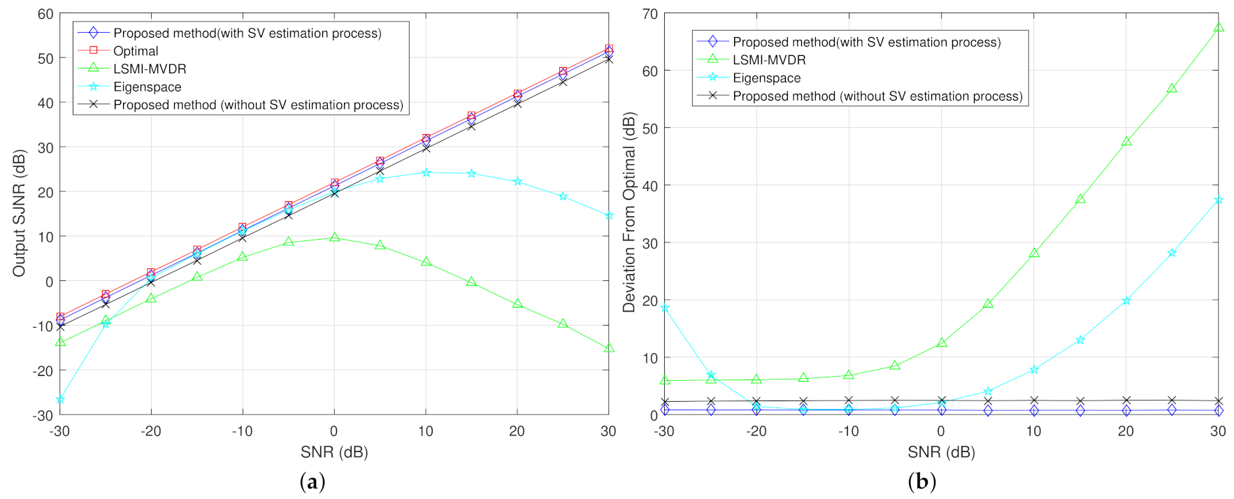
- We propose a novel robust mainlobe deceptive target suppression method based on covariance matrix reconstruction to suppress the deceptive targets in the mainlobe. First, the proposed method reconstructs the deceptive targets and noise covariance matrix with the Capon power spectrum over the complementary region of the desired target region (DTR). Therefore, the reconstructed covariance matrix only collects information about deceptive targets and noise. Then, similarly, the covariance matrix of the desired target including the steering vector (SV) information of the desired target is constructed through integrating the Capon power spectrum over the DTR. The transmit–receive SV of the desired target is estimated as the dominant eigenvector of the desired target covariance matrix. Finally, the weighting vector of the receive beamformer is calculated by combining the reconstructed jammer-noise covariance matrix (JNCM) and the estimated desired target SV.
2. FDA-MIMO Signal Model
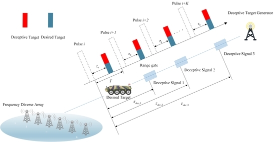
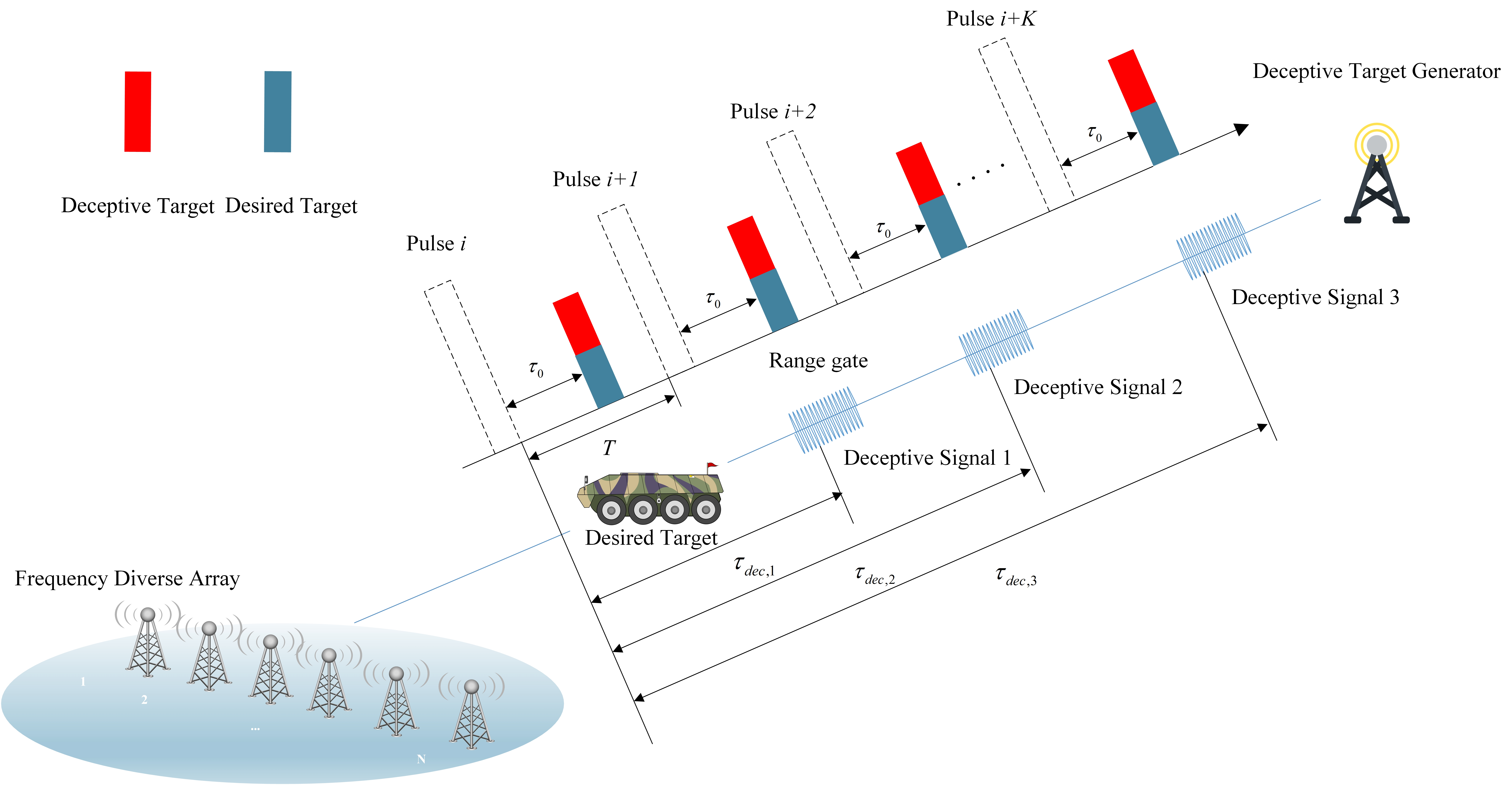
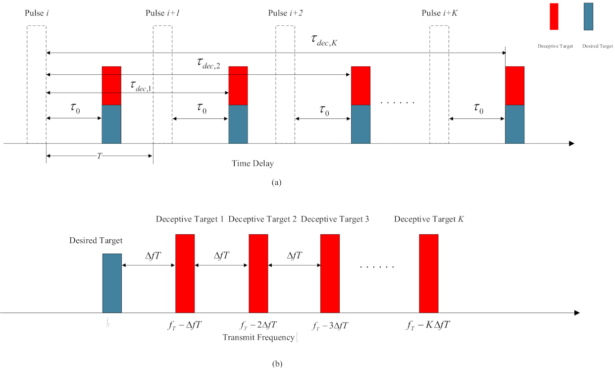
3. Model of Range Ambiguious Deceptive Jammer
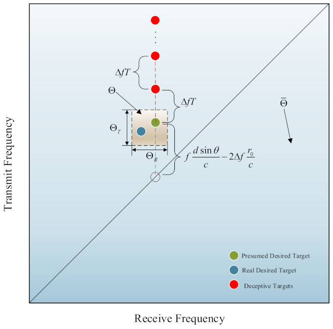
4. Robust Ambiguous Range Deceptive Target Suppression Based on Covariance Matrix Reconstruction
5. Simulation
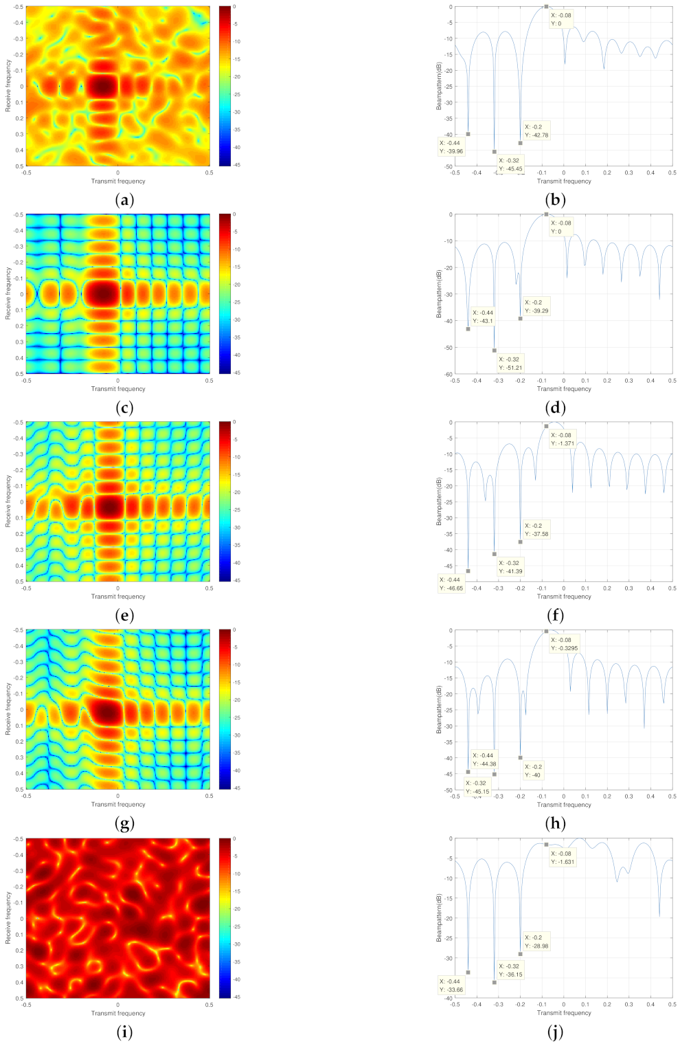
5.1. Example 1
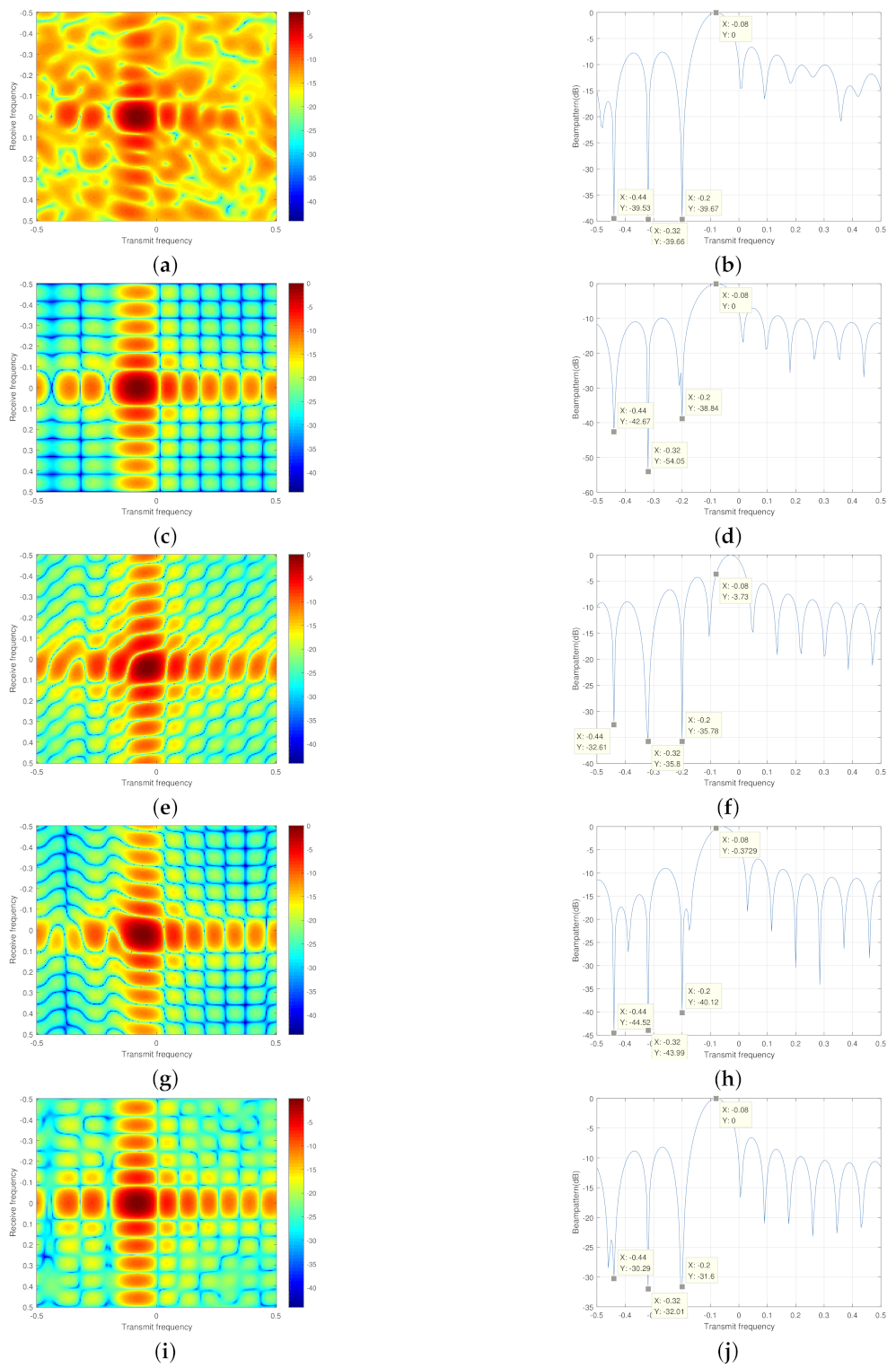
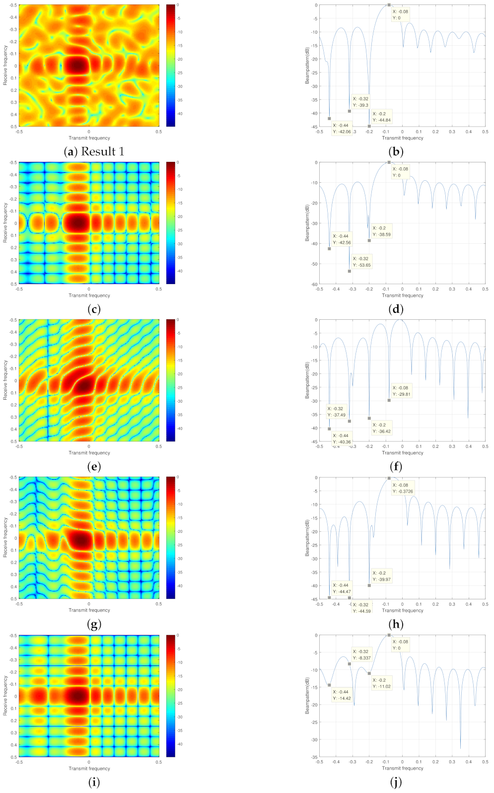
5.2. Example 2
6. Conclusions
Author Contributions
Funding
Conflicts of Interest
References
- Antonik, P.; Wicks, M.C.; Griffiths, H.D.; Baker, C.J. Range-dependent beamforming using element level waveform diversity. In Proceedings of the 2006 International Waveform Diversity Design Conference, Lihue, HI, USA, 22–27 January 2006; pp. 1–6. [Google Scholar]
- Antonik, P.; Wicks, M.C.; Griffiths, H.D.; Baker, C.J. Multi-mission multi-mode waveform diversity. In Proceedings of the 2006 IEEE Conference on Radar, Verona, NY, USA, 24–27 April 2006; p. 3. [Google Scholar]
- Wang, W. Frequency Diverse Array Antenna: New Opportunities. IEEE Antennas Propag. Mag. 2015, 57, 145–152. [Google Scholar] [CrossRef]
- Secmen, M.; Demir, S.; Hizal, A.; Eker, T. Frequency Diverse Array Antenna with Periodic Time Modulated Pattern in Range and Angle. In Proceedings of the 2007 IEEE Radar Conference, Waltham, MA, USA, 17–20 April 2007; pp. 427–430. [Google Scholar]
- Khan, W.; Qureshi, I.M. Frequency Diverse Array Radar with Time-Dependent Frequency Offset. IEEE Antennas Wirel. Propag. Lett. 2014, 13, 758–761. [Google Scholar] [CrossRef]
- Xu, Y.; Shi, X.; Xu, J.; Li, P. Range-Angle-Dependent Beamforming of Pulsed Frequency Diverse Array. IEEE Trans. Antennas Propag. 2015, 63, 3262–3267. [Google Scholar] [CrossRef]
- Yao, A.; Wu, W.; Fang, D. Frequency Diverse Array Antenna Using Time-Modulated Optimized Frequency Offset to Obtain Time-Invariant Spatial Fine Focusing Beampattern. IEEE Trans. Antennas Propag. 2016, 64, 4434–4446. [Google Scholar] [CrossRef]
- Yao, A.; Rocca, P.; Wu, W.; Massa, A.; Fang, D. Synthesis of Time-Modulated Frequency Diverse Arrays for Short-Range Multi-Focusing. IEEE J. Sel. Top. Signal Process. 2017, 11, 282–294. [Google Scholar] [CrossRef]
- Wang, Y.; Li, W.; Huang, G.; Li, J. Time-Invariant Range-Angle-Dependent Beampattern Synthesis for FDA Radar Targets Tracking. IEEE Antennas Wirel. Propag. Lett. 2017, 16, 2375–2379. [Google Scholar] [CrossRef]
- Chen, B.; Chen, X.; Huang, Y.; Guan, J. Transmit Beampattern Synthesis for the FDA Radar. IEEE Antennas Wirel. Propag. Lett. 2018, 17, 98–101. [Google Scholar] [CrossRef]
- Fishler, E.; Haimovich, A.; Blum, R.; Chizhik, D.; Cimini, L.; Valenzuela, R. MIMO radar: An idea whose time has come. In Proceedings of the 2004 IEEE Radar Conference (IEEE Cat. No.04CH37509), Philadelphia, PA, USA, 29 April 2004; pp. 71–78. [Google Scholar]
- Davis, M.S.; Showman, G.A.; Lanterman, A.D. Coherent MIMO radar: The phased array and orthogonal waveforms. IEEE Aerosp. Electron. Syst. Mag. 2014, 29, 76–91. [Google Scholar] [CrossRef]
- Liu, W.; Wang, Y.; Liu, J.; Xie, W.; Chen, H.; Gu, W. Adaptive detection without training data in colocated MIMO radar. IEEE Trans. Aerosp. Electron. Syst. 2015, 51, 2469–2479. [Google Scholar] [CrossRef]
- Wen, C.; Tao, M.; Peng, J.; Wu, J.; Wang, T. Clutter Suppression for Airborne FDA-MIMO Radar Using Multi-Waveform Adaptive Processing and Auxiliary Channel STAP. Signal Process. 2019, 154, 280–293. [Google Scholar] [CrossRef]
- Wang, C.; Xu, J.; Liao, G.; Xu, X.; Zhang, Y. A Range Ambiguity Resolution Approach for High-Resolution and Wide-Swath SAR Imaging Using Frequency Diverse Array. IEEE J. Sel. Top. Signal Process. 2017, 11, 336–346. [Google Scholar] [CrossRef]
- Sammartino, P.F.; Baker, C.J.; Griffiths, H.D. Frequency Diverse MIMO Techniques for Radar. IEEE Trans. Aerosp. Electron. Syst. 2013, 49, 201–222. [Google Scholar] [CrossRef]
- Vorobyov, S.A.; Gershman, A.B.; Luo, Z.-Q. Robust adaptive beamforming using worst-case performance optimization: A solution to the signal mismatch problem. IEEE Trans. Signal Process. 2003, 51, 313–324. [Google Scholar] [CrossRef]
- Xu, J.; Liao, G.; Zhu, S.; So, H.C. Deceptive jamming suppression with frequency diverse MIMO radar. Signal Process. 2015, 113, 9–17. [Google Scholar] [CrossRef]
- Lan, L.; Liao, G.; Xu, J.; Zhang, Y.; Fioranelli, F. Suppression Approach to Main-Beam Deceptive Jamming in FDA-MIMO Radar Using Nonhomogeneous Sample Detection. IEEE Access 2018, 6, 34582–34597. [Google Scholar] [CrossRef]
- Shi, J.; Liu, X.; Yang, Y.; Sun, J.; Wang, N. Comments on “Deceptive jamming suppression with frequency diverse MIMO radar”. Signal Process. 2018, 158, 1–3. [Google Scholar] [CrossRef]
- Akhtar, J.; Olsen, K.E. Frequency agility radar with overlapping pulses and sparse reconstruction. In Proceedings of the 2018 IEEE Radar Conference (RadarConf18), Oklahoma City, OK, USA, 23–27 April 2018; pp. 0061–0066. [Google Scholar]
- Xiang, Z.; Chen, B.; Yang, M. Transmitter/receiver polarisation optimisation based on oblique projection filtering for mainlobe interference suppression in polarimetric multiple-input–multiple-output radar. IET Radar Sonar Navig. 2018, 12, 137–144. [Google Scholar] [CrossRef]
- Ding, L.; Li, R.; Wang, Y.; Dai, L.; Chen, F. Discrimination and identification between mainlobe repeater jamming and target echo by basis pursuit. IET Radar Sonar Navig. 2017, 11, 11–20. [Google Scholar] [CrossRef]
- Li, J.; Stoica, P. MIMO Radar Signal Processing; John Wiley & Sons: Hoboken, NJ, USA, 2008. [Google Scholar]
- Gu, Y.; Leshem, A. Robust adaptive beamforming based on interference covariance matrix reconstruction and steering vector estimation. IEEE Trans. Signal Process. 2012, 60, 3881–3885. [Google Scholar]
- Zheng, Z.; Yang, T.; Wang, W.Q.; So, H.C. Robust adaptive beamforming via simplified interference power estimation. IEEE Trans. Aerosp. Electron Syst. 2019, 55, 3139–3152. [Google Scholar] [CrossRef]


| Parameter | Value | Parameter | Value |
|---|---|---|---|
| Size of the array | 10 | Noise power | 0 dB |
| Reference carrier frequency | 1.5 GHz | Real target angle | |
| Pulses per CPI | 400 | Assumed target angle | |
| Frequency increment | 2 KHz | Target range | 6 km |
| PRF | 33 KHz | JNR | 30 dB |
Publisher’s Note: MDPI stays neutral with regard to jurisdictional claims in published maps and institutional affiliations. |
© 2021 by the authors. Licensee MDPI, Basel, Switzerland. This article is an open access article distributed under the terms and conditions of the Creative Commons Attribution (CC BY) license (https://creativecommons.org/licenses/by/4.0/).
Share and Cite
Xie, Z.; Zhu, J.; Fan, C.; Huang, X.; Wang, J. Robust Range Ambiguous Deceptive Target Suppression Based on Covariance Matrix Reconstruction. Remote Sens. 2021, 13, 2346. https://doi.org/10.3390/rs13122346
Xie Z, Zhu J, Fan C, Huang X, Wang J. Robust Range Ambiguous Deceptive Target Suppression Based on Covariance Matrix Reconstruction. Remote Sensing. 2021; 13(12):2346. https://doi.org/10.3390/rs13122346
Chicago/Turabian StyleXie, Zhuang, Jiahua Zhu, Chongyi Fan, Xiaotao Huang, and Jian Wang. 2021. "Robust Range Ambiguous Deceptive Target Suppression Based on Covariance Matrix Reconstruction" Remote Sensing 13, no. 12: 2346. https://doi.org/10.3390/rs13122346
APA StyleXie, Z., Zhu, J., Fan, C., Huang, X., & Wang, J. (2021). Robust Range Ambiguous Deceptive Target Suppression Based on Covariance Matrix Reconstruction. Remote Sensing, 13(12), 2346. https://doi.org/10.3390/rs13122346