Abstract
This paper describes a novel technique for estimating how many mines remain after a full or partial underwater mine hunting operation. The technique applies Bayesian fusion of all evidence from the heterogeneous sensor systems used for detection, classification, and identification of mines. It relies on through-the-sensor (TTS) assessment, by which the sensors’ performances can be measured in situ through processing of their recorded data, yielding the local mine recognition probability, and false alarm rate. The method constructs a risk map of the minefield area composed of small grid cells (~4 m2) that are colour coded according to the remaining mine probability. The new approach can produce this map using the available evidence whenever decision support is needed during the mine hunting operation, e.g., for replanning purposes. What distinguishes the new technique from other recent TTS methods is its use of Bayesian networks that facilitate more complex reasoning within each grid cell. These networks thus allow for the incorporation of two types of evidence not previously considered in evaluation: the explosions that typically result from mine neutralization and verification of mine destruction by visual/sonar inspection. A simulation study illustrates how these additional pieces of evidence lead to the improved estimation of the number of deployed mines (M), compared to results from two recent TTS evaluation approaches that do not use them. Estimation performance was assessed using the mean squared error (MSE) in estimates of M.
1. Introduction
Sea mines constitute a formidable threat to commercial shipping and naval operations because these weapons are highly effective, low-cost, easy to employ, covert, and widely available [1]. The primary method to address this threat is through mine sweeping and mine hunting, collectively known as mine countermeasures (MCM). While sweeping is focused on actuating the mines using mechanical or influence methods, mine hunting is a multi-phase process that systematically searches for, identifies, and neutralizes mines. Mine hunting requires the fusion of multiple data processing results from heterogeneous sensors and platforms. The role of MCM evaluation is to assess the overall performance and to communicate the remaining risk to decision makers. Improving the evaluation of mine hunting is the focus of this work.
Recent developments in sensing, robotics, and perception algorithms, such as automatic target recognition (ATR), have drastically changed the conduct of mine hunting. Modern autonomous underwater vehicles (AUVs) equipped with advanced side looking sonar systems (SLS), either side scan sonar (SSS) or synthetic aperture sonar (SAS), have become essential platforms in mine hunting [2]. Such vehicles provide superior data quality, improved efficiency, covertness, and reduced risk to personnel [2,3]. Increasingly, these AUVs have sufficient processing power to run perception algorithms during data collection, and to alter their own behaviour in situ, in response, for example, to ATR results [4]. The employment of robotic systems has required fundamental changes to the execution of mine hunting, shifting from a process where one vessel conducts search, classification, identification, and neutralization to one where robotic and human systems work collaboratively [5,6]. Thus, tasks are now usually accomplished in a different order and are often undertaken concurrently.
In the initial search phase of modern mine hunting, AUVs survey a potential threat area using high-resolution SLS to detect and classify mine-like contacts (MILCOs) in acoustic images of the seafloor. These contacts are then reacquired using a remotely operated vehicle (ROV), diver, or AUV to be identified using optical sensors, as either a MINE or a NOMBO (Non-mine mine-like bottom object). The most common technique for neutralizing the threat of an identified mine is to set it off with a small explosive charge deposited by an ROV, a diver, or a mine disposal weapon. Explosive neutralization can be verified either by observing the detonation’s effect on the sea surface or by re-inspecting the object’s location (visually or with sonar). The size of the explosion that results from mine neutralization provides the indirect evidence that the mine was disabled; however, it is possible that the deposited charge disables the mine without actuating it. If neutralization failure is suspected, further inspection (by diver, ROV or AUV) can reveal whether the mine was really destroyed, or a new charge can be laid to repeat the neutralization attempt.
The modern approach of executing the individual phases of mine hunting independently provides advantages, from protecting humans from harm in the minefield, to mapping areas where low risk transit is possible [7]. On the other hand, it poses significant challenges to the fusion of platform, sensing, and perception performances to determine the overall effectiveness of the process. Reliable estimates of mine hunting effectiveness are essential, both for planning further MCM efforts in the area and for quantifying the risk remaining to subsequent traffic. Traditionally, quantifying that risk has been the primary role of MCM evaluation [8]. The operational differences between ship-based and robotic mine hunting systems necessitate a revision of the prevailing methods and metrics used for effectiveness evaluation [9].
The traditional Bayesian models used in MCM evaluation within the NATO alliance rely on an index of effectiveness called the percentage clearance [8]. This metric measures the average probability of clearing a given mine over the entire minefield area. It depends mainly on the effectiveness of the search sonar in the environment. As an overall average, the percentage clearance can conceal a lot of local variation [9]. Furthermore, traditional models required all phases of mine hunting to be completed in order to estimate the residual risk [8].
The ability of modern systems to record large amounts of geo-referenced sensor data is well suited to a new approach to MCM evaluation that provides high-fidelity performance estimates during mission execution. This new approach is called through-the-sensor (TTS) evaluation. The idea is to measure the local performance of the SLS sensors in situ by processing their own measurements to derive meaningful performance indices. The TTS approach is of greatest value when relevant conditions vary rapidly in space or time. The result of this technique is encoded in a georeferenced grid, providing a high-resolution view of the phase performance.
Several studies have addressed the data-driven evaluation of SLS survey performance using the probability of mine detection and classification, pDC, and the probability of false alarm, pFA [3,10,11,12]. Because complex dependencies make it difficult to derive the two performance indices directly from the sonar image data, most methods calculate a set of latent parameters within small image windows, and then apply a learned mapping to get from these parameter values to pDC and pFA. The various approaches differ in both the choice of latent parameters and the training of mapping functions using real and/or simulated sonar data.
To produce a complete metric of MCM performance, the uncertainties and performances of all executed phases must be fused. A recent study [5] derived Bayesian formulations to extend grid-based TTS evaluation of the search phase to include the contact identification and mine neutralization phases, and introduced a new MCM metric, the probability of a remaining mine in the given cell. Comparable formulations were also presented in [6], although these did not consider mine neutralization as explicitly. To compute this local probability, one approach involves embedding a probabilistic model into each cell of a detailed geographical grid. This model can then evaluate the outcomes of the MCM effort within the grid cell and estimate the probability that a mine remains there [5]. The key contribution of this paper is to have Bayesian networks provide that probabilistic model within each cell, facilitating more complex reasoning than in [5,6].
Bayesian networks are graph-based probabilistic models that have been used extensively for the development of decision making and expert systems. They are seeing increasing use in geographical applications [13], such as the mapping of mining potential [14], cliff erosion [15], or flooding [16]. They are considered to have improved environmental risk mapping [17], a field in which there are a large number of applications like [18], many more of which are reviewed in [19]. The applications of Bayesian networks to spatial mapping have grown so common that a recent doctoral thesis categorizes them into several approaches, under the label of spatial Bayesian networks [20]. Under the proposed categorization, the current application would be classed as one in which “spatial units are represented as instances of the network”. The other categories are “spatial units represented by network nodes” and “network with a spatial node”. The doctoral thesis contains helpful figures illustrating the difference between these approaches.
Bayesian networks can effectively encode causal relationships and inherently have an ability to reason under uncertainty over multiple random variables [21]. These networks permit the consideration of evidence related to mine neutralization provided by explosions and by verification efforts. Such evidence has not previously been considered in MCM evaluation.
By leveraging the gridded TTS performance measurement from [3], combined with mine remaining estimates from the embedded Bayesian networks, this paper will demonstrate a novel capability for MCM evaluation. It will show that using the new evidence from the neutralization phase increases the fidelity of performance evaluation. This will be accomplished by comparing results with those obtained from the methods in [5] and [6] on simulated datasets.
As the primary aim of MCM evaluation is to quantify the risk to follow-on traffic [8], the remaining mine probability grid from this work facilitates high fidelity risk maps and lends itself to the selection of shipping routes to minimize risk [7]. By using Bayesian networks to leverage the advanced capabilities provided by TTS evaluation, which considers platform, sensing, and ATR performance, the proposed method can move beyond post-mission evaluation to provide situational awareness throughout mine hunting operations. It can also help prioritize tasks.
The remainder of this work is structured as follows: Section 2 will introduce the use of Bayesian networks to the MCM problem and illustrate the gridded approach taken; Section 3 will present the design of the simulation study comparing methods; Section 4 will present the simulation study results; and Section 5 will present conclusions and areas of future work.
2. Methods
This paper presents a new approach based on Bayesian networks that permits users to evaluate MCM performance. A Bayesian network is a graphical model of the conditional dependencies between a set of discrete random variables, each represented by a network node [22]. Bayesian networks are interactive tools that permit users to enter evidence on any node or set of nodes. Such evidence consists of a configuration of states for all the nodes in the evidence set. Once such evidence is entered, Bayesian networks offer three core capabilities related to that evidence. The first and most used capability is to propagate the evidence to any other node in the network, computing the marginal probability table for that node given the evidence. The second capability is to compute the probability of the entered evidence. The final capability is to simulate a random configuration of states for any set of nodes (outside of the evidence set) that is consistent with the entered evidence. Such consistency means that the configuration is drawn randomly from the joint posterior probability distribution for the node set, given the evidence. All three capabilities are used in this paper: the first and third in the pseudocode of Section 2.4, the second in Section 2.3. The Bayesian networks in this paper were implemented using the (free) demo version of the Hugin tool [23] and especially its accompanying application program interface.
The following subsections outline the application of Bayesian networks to measuring MCM performance, with the primary goal being to predict the probabilities of remaining mines after the execution of MCM effort. These probabilities are a key component of predicting risk in a geographic area. To accomplish this prediction, a segmentation of the area will be made, followed by an assignment of a Bayesian network to each cell. Since the approach is Bayesian, it requires a prior distribution, in this case for the probability of a mine in each cell. This paper suggests using a uniform prior. Once the prior is set, it allows for the prediction of the posterior probability of a mine in each individual grid cell from Bayes’ Theorem.
2.1. Applying a Mine Probability Model to a Spatial Grid of the Mined Area
It is assumed here that the minefield has been divided up into C small grid cells. Each of these cells is small enough that it may reasonably be taken to contain at most one MILCO or mine. This one object per cell assumption is more realistic, if the cells are relatively small. On the other hand, the cells should not be so small that mines would often span multiple cells. Given these conflicting considerations, a cell size of 2 m × 2 m was selected. This choice implies the minefield will typically contain many cells: a minefield that was 2 km long and 1 km wide, for example, would have 500,000 cells.
Let pM denote the probability of there being a mine in a cell. A uniform Bayesian prior is assigned to pM. As this prior is cut off at max(pM) < 1, it effectively imposes an upper limit on the number of mines deployed. To set max(pM), consider that it is inefficient for mine layers to place mines so that their blast radii overlap because the blast from one mine could render the other ineffective, and hence they could exclude more areas by deploying the extra mines elsewhere. This paper took the blast radius of mines to be 60 m. Then, a 2 km long and 1 km wide minefield could contain 128 disjoint disks of radius 60 m, in 8 rows of 16. Thus, this paper used max(pM) = 128/500,000 throughout.
Let the discrete, random variable m(c) be equal to 1, if there really is a mine in cell c, and equal to 0, if there is no mine present. Let M denote the total number of mines deployed. In estimation, mines are treated as if they arose from the hierarchical model shown in Figure 1.
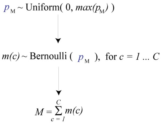
Figure 1.
The core hierarchical model used in estimation. Mines will be treated as if they arose from this model.
2.2. Assigning a Bayesian Network to Each Cell
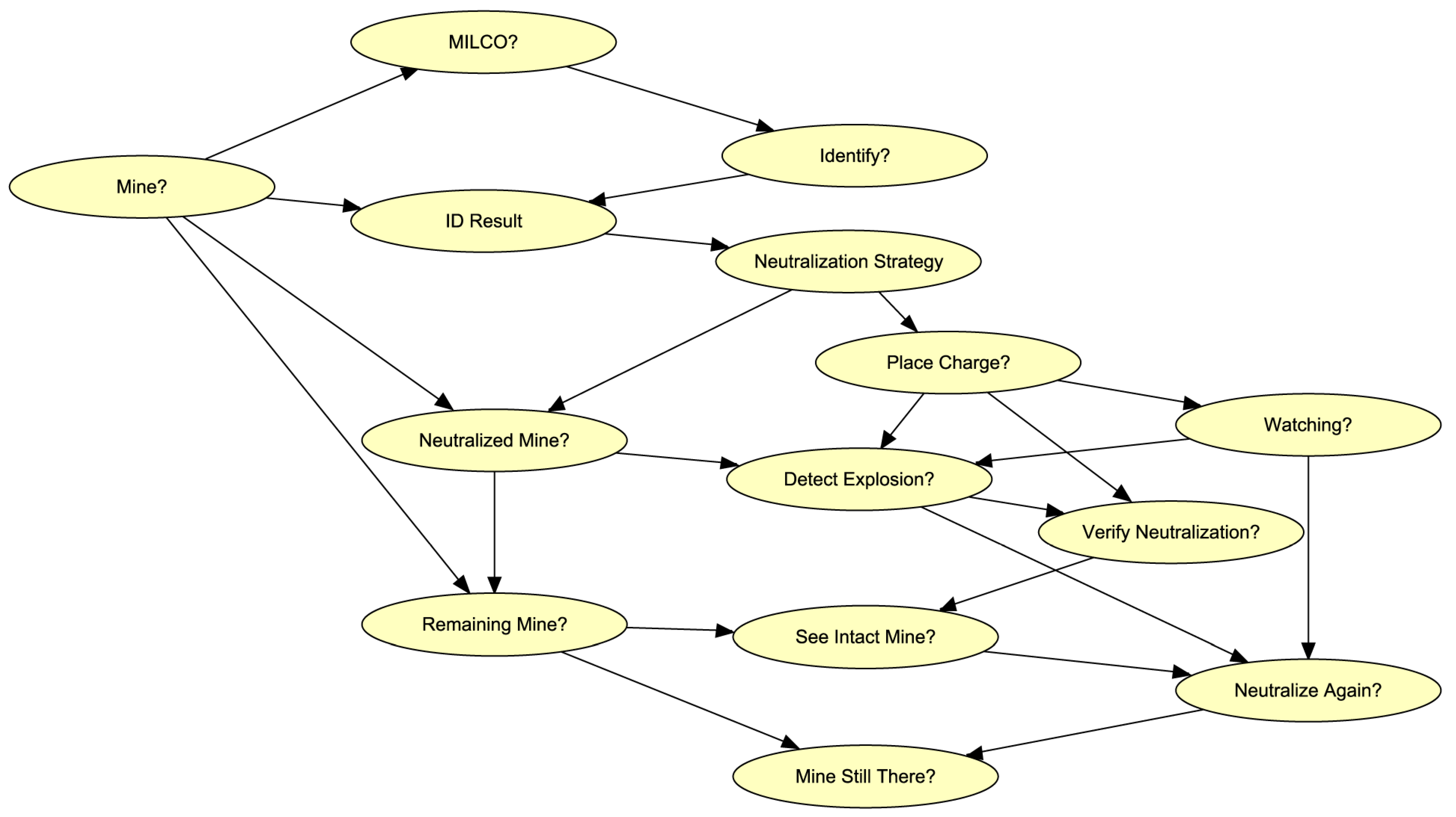
The key idea of the approach here is to assign a Bayesian network to each grid cell in order to process the local evidence within that cell. The nodes in these networks are interpreted as shown in Table 1. The directed acyclic graph (DAG) for each network is depicted in Figure 2. The DAG represents the causal relationships between the discrete random variables in the network using arrows. Thus, for example, the probability that there is a MILCO in a cell, which is represented by the ‘MILCO?’ node, is determined by whether there really is a mine (as represented by the ‘Mine?’ node). Unlike many Bayesian network applications, where the direction of the arrows can be uncertain, here the arrows follow the temporal order in which observations are obtained. First, the MILCOs are detected, then the selected ones are identified, then some of those are neutralized, after which there might be explosions and attempts at verification, and so on. Thus, the DAG model uncertainty is lower than in many other applications of Bayesian networks [24]. Note that the Boolean ‘Mine?’ node is an alias for m(c) in Figure 1.

Table 1.
The nodes of the Bayesian network.
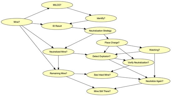
Figure 2.
This directed acyclic graph provides both the discrete random variables (represented as yellow ellipses) used to model inference within each grid cell and the causal relationships between them (represented with arrows). The graph forms the basis of a Bayesian network. That network uses the convention that Boolean random variables have names ending with a question mark.
Table 2 provides a list of the parameters needed to turn the DAG in Figure 2 into a Bayesian network. These are used to create conditional probability tables. The details of where these parameters appear in these tables are given in Figure A1, Figure A2 and Figure A3 (Appendix A). The parameters above the solid line in Table 2 have to do with the performance of sensors and processes, while those below predict the decisions of mine warfare officers. Only the parameters above the line affect MCM evaluation results. Those below are only important for the purpose of simulating datasets (consider skipping those on first reading). The Bayesian networks are almost the same in each cell. The only difference between them is in the probability table for the ‘MILCO?’ node. As shown in Figure A1 (Appendix A), this table reflects the local pDC and pFA values that are measured through the sensor within each grid cell (see Table 2). All the other probability tables are identical in each cell.
Table 2.
This table provides a glossary of network parameters. Those above the solid line control the performance of sensors and processes, while those below are used to predict the decisions of mine warfare officers (in simulation). These decisions concern which MILCOs to identify, which identified mines to neutralize (and how to do it), whether to investigate further and whether to retry neutralization (when it might have failed).
2.3. Using a Grid Approach to Estimate pM
The most difficult parameter to estimate is pM because this estimation is not handled by the Bayesian networks. This paper suggests using a grid approach. To construct the required grid of pM values, consider the maximum possible value for this parameter, denoted by max(pM). A grid can readily be formed by creating an array of G evenly spaced values for pM between 0 and max(pM). Let the distinct values in this grid be denoted by pM(g), for grid index g running from 1 to G. This paper took the grid length to be G = 129, since max(pM) = 128/500,000, to facilitate comparison to PESOS results (the ‘Planning and Evaluation System of Systems’ (PESOS) is based on [6]), which use that same grid.
At each value of pM(g) in this grid, all C of the 2 m × 2 m grid cells are independent (recall the conditional independence property of the model in Figure 1). Thus, the likelihood of the evidence in all the cells, conditional on pM(g), is given by the product of the likelihood of the evidence in each individual cell. This is convenient because the likelihood of the evidence in a cell is readily computed by the Bayesian network in that cell, provided that the ‘Mine?’ table is updated to include pM(g).
Table 3 provides some common evidence configurations to enter on the network. In this paper, a set of evidence in a cell always includes states for all the nodes on the left margin of Table 3. Hence, a likelihood score is readily computed for each distinct value of pM(g). Naturally, the final posterior score (s(pM(g))) is given by the product of the likelihood and the prior evaluated at pM(g), in accordance with Bayes’ theorem.
Table 3.
State configurations for the nodes in the left column under a variety of common forms of evidence. That evidence represents the observations available within a particular grid cell.
In a departure from typical Bayesian practice, this paper suggests using a point estimate for pM, rather than the usual posterior distribution. The reason for this shortcut is to allow other parameters of interest to be estimated using just a single Bayesian network in each grid cell, as opposed to having to average results over multiple networks. Using a single network makes the computations faster (G times faster to be precise) and thus more interactive for users. Note that it certainly would be possible to satisfy Bayesian purists by continuing to average results over G networks (one for each value of pM(g)), weighting each network by its posterior score s(pM(g)), in all subsequent inference, but the loss in speed is not adequately compensated. The suggested point estimate is as follows:
In Equation (1), the posterior scores s(pM(g)) are computed as suggested in the previous two paragraphs. Subsequent estimation results are then computed by entering in place of pM in the ‘Mine?’ table (in all the grid cells).
2.4. Using Monte Carlo Simulation to Estimate M
As mentioned above, the Bayesian network depicted in Figure 2 can simulate data that is compatible with entered evidence. Thus, it can generate a sample of values for all the nodes in Table 1 that is compatible with any given set of evidence. This Monte Carlo simulation capability will be used here to estimate the total number of mines initially deployed, as well as the total number remaining. The process takes several steps, which are given in the following pseudocode:
- Create an integer array M[i], indexed by i = 1 to 1000. Initialize this array to all 0 entries.
- Create an integer array R[i], indexed by i = 1 to 1000. Initialize this array to all 0 entries.
- Loop over the grid cells, for c = 1 to C, performing steps a and b below:
- a.
- Within grid cell c, enter the evidence e that is available within c on the local network.
- b.
- For i = 1 to 1000, do steps i, ii, and iii below:
- i.
- Generate a sample s of node values from the Bayesian network that is compatible with e.
- ii.
- Let M[i] = M[i] + 1, if the value of the ‘Mine?’ node is ‘True’ in the sample s and make no change to M[i] otherwise.
- iii.
- Let R[i] = R[i] + 1, if the value of the ‘Mine Still There?’ node is ‘True’ in the sample s and make no change to R[i] otherwise.
Once these steps are complete, the M[i] array provides a sample of size 1000 for the number of mines initially deployed (in all the cells), while the R[i] array provides a similar sample for the number of mines remaining.
3. Simulation Study Design
This paper includes a simulation study (not to be confused with using Monte Carlo simulation to estimate the number of mines deployed, M, as described in Section 2.4), in which the Bayesian networks were used to simulate 40 partially-processed minefield datasets. These simulated minefields were usually partially processed because they allowed for the possibility of leaving a MILCO or an identified mine unprocessed (see the ‘Identify?’ and ‘Neutralization Strategy’ tables in Figure A1 (Appendix A)). The estimation approach described above (named ‘Bayes Net’) was applied to each of these datasets to see how well it would do at recovering the simulated value of M. Its performance was compared to that of other methods based on equations proposed in [5,6], which are referred to as ‘Bayes Global’ and ‘PESOS’, respectively. Performance was examined primarily in terms of the Mean Squared Error (MSE) in estimating M, but posterior mean bias and posterior mode bias for M were also computed for each method.
3.1. The Bayes Global and Bayes Global+ Approaches
The Bayes Global technique described in Equation (6) of [5] assumes that all MILCOs have been identified. If the technique is applied to a minefield dataset in which some of the MILCOs are left unidentified (as it will be below), these MILCOs will be interpreted as NOMBOs, thereby biasing estimates of the number of mines deployed, M, downwards. This paper thus proposes a relatively small enhancement, named ‘Bayes Global+’, to rectify this negative bias. The description of the Bayes Global+ approach is aided by a quick review of Bayes Global.
The Bayes Global method estimates M based on average values for the TTS parameters taken over the minefield grid. These average values are denoted by and , respectively, for the mine detection probability and false alarm rate. It also applies a number of statistics obtained by adding up results in all the grid cells: the total number of MILCOs (mDC) and the total of identified mines (mI). The Bayes Global+ enhancement also applies the total number of MILCOs left unidentified (mL). Finally, Bayes Global uses a number of parameters defined above in Table 2, namely pI, pRI and pIFA. Recall that the total number of grid cells is C.
The description of the Bayes Global methods is facilitated by the following notation for the Binomial probability mass function:
The Bayes Global method assigns to each possible number of mines deployed (M) a likelihood score proportional to the following:
The Bayes Global+ method assigns to each possible M a likelihood score proportional to the following:
When all MILCOs are identified (mL = 0), Equation (4) degenerates into Equation (3). Note that the final scores would be proportional to the product of the likelihood (t or t′) and the prior assigned to M, in accordance with Bayes’ theorem.
3.2. Details of Minefield Simulation
As mentioned above, the simulation study used the Bayesian network of Figure 2 to simulate a partially processed minefield. This section provides the details of how that was conducted.
For simulation, pM was taken to be 15/500,000, so there should be approximately 15 mines in each dataset, on average. Simulation handled each grid cell (c) in turn. Values of pDC and pFA within cell c were drawn randomly from a Beta(18, 2) distribution, for the former (mean 90%), and from a Beta(1,9999), for the latter (mean 0.01%). The probability table for the ‘MILCO?’ node (see Figure A1 (Appendix A)) was then edited to reflect those local values of pDC and pFA. The other Bayesian network parameter values were set as given in the second column of Table 2. Then, the simulation capability of Bayesian networks was used to compute the ground truth in each cell (values for the ‘Mine?’, ‘Neutralized Mine?’, ‘Remaining Mine?’ and ‘Mine Still There?’ nodes), as well as the evidence used in estimation (values for all the other nodes). Finally, the simulated value of M was determined by counting the number of grid cells in which the ‘Mine?’ node was in state TRUE.
3.3. Evidence Available in Estimation
The evidence available in estimation varied by the approach used. For the Bayesian networks, that evidence consisted of values for all the nodes on the left margin of Table 3 in each grid cell. For the PESOS approach, the evidence consisted of whether there is a MILCO in the cell and, when there was one that was also visually identified, whether it was identified as a MINE or as a NOMBO. For the Bayes Global and Bayes Global+ approaches, the evidence consisted of the total number of MILCOs and identified MINEs over all the cells. The Bayes Global+ method also needed the total number of MILCOs left unidentified (see Equations (3) and (4) above). Note that the PESOS and Bayes Net estimation models had access to the exact values of pDC and pFA in each cell, while the Bayes Global and Bayes Global+ methods used the mean values of these parameters. The Bayes Net approach also had access to all the parameter values specified in the second column of Table 2. In contrast, the other approaches only needed the values of pI, pRI and pIFA from that table. The simulation study added a sensitivity analysis for eW, as it was considered a likely source of Bayes Net advantage.
3.4. Sensitivity Analysis
The simulation study included an investigation of the effects of using incorrect values for eW in Bayes Net estimation. Recall (from Table 2) that this parameter represents the probability that a neutralized mine will result in an explosion that is detected at the sea surface, in the situation that such an explosion is expressly watched for. In the simulated datasets, explosions were watched for in w = 95% of mine neutralizations. In the simulated datasets, eW was taken to be 90%. Thus, the study examined the impacts of using incorrect values of eW = 95% and 80% in estimation, as compared to using the correct value. The former value would give too much weight to the explosion evidence, while the latter would give too little.
4. Results
Figure 3 gives the scores computed over the grid defined in Section 2.3 using the first simulated dataset. In that figure, the posterior density for pM evaluated at pM(g) would be proportional to the score s(pM(g)). Note that this figure also compares the grid scores to the scores resulting from Equation (2) of [6], under the PESOS label. The scores are similar but not quite the same. Note that the PESOS approach only uses evidence from the ‘MILCO?’ and ‘ID Result’ nodes (see Section 3.3), whereas the Bayesian networks use all the evidence from the nodes on the left margin of Table 3, so it is natural that results would differ. To highlight the source of the difference, the results were recomputed for the Bayes Net approach (on a second simulated dataset) using only evidence from the ‘MILCO?’ and ‘ID Result’ nodes. In that case, the Bayes Net and PESOS posteriors were identical (to 13 decimal places), providing reassuring validation. This implies that the difference between the scores in Figure 3 is a result of using the additional evidence, not a result of the Bayesian networks themselves.
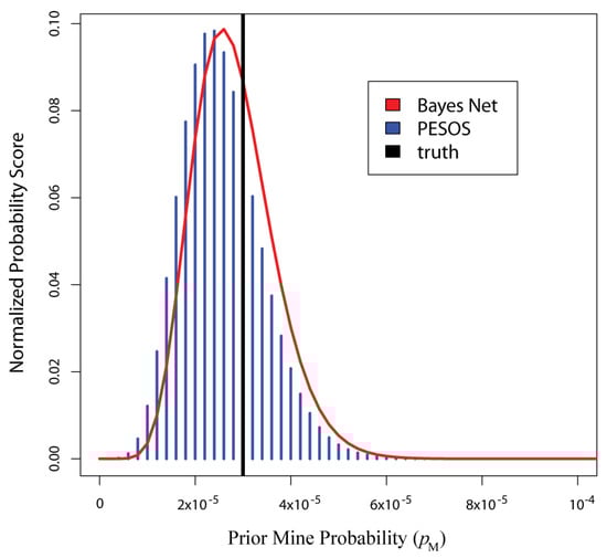
Figure 3.
This figure gives the posterior scores computed over the 129 grid points of pM(g) using both the Bayes Net and PESOS approaches. These results were computed using the first simulated dataset.
4.1. The Effects of Explosions and Verification
The previous section showed that the Bayesian networks provide results practically identical to those from Equation (2) of [6], when they both use the same evidence. The aim of this section is to reveal the effects of considering additional evidence, beyond the MILCOs and identified mines. To suggest how the Bayesian networks handle such evidence, this paper uses a typical Bayesian network, with values for pM, pDC, and pFA set at average values for the simulation design outlined in Section 3.2. These values were pM = 15/500,000, pDC = 90%, and pFA = 0.01%. Other values were as given in Table 2. Interest centers on the effects of different evidence on the probability that the ‘Mine?’ node is in state True, described as the mine probability below.
Observing a MILCO in a cell raises the mine probability from 0.003% to 21.26%. Identifying that MILCO as a mine raises the mine probability further to 93.04%. So far, these results are in line with the approaches in [5] and [6]. If mine warfare officers decide to neutralize that target with the same robot that identified it as a MINE and decide to watch for explosions (so ‘Watching?’ is True), they may see an explosion (probability 82.98%) or may not (17.02%). If they do see one (‘Detect Explosion?’ is True), the mine probability rises to 99.92% (it is not quite certain because the observed explosion might just have resulted from the detonation charge itself rather than from a real mine explosion), but if they do not, it falls to 59.52%. The lack of explosion casts doubts on whether there was a mine to begin with, while the explosion all but confirms it (since a neutralized mine would explode 90% of the time). Supposing they don’t see one, they are likely to perform an inspection to throw additional light on the matter because there is a 45.89% chance that ‘Neutralized Mine?’ is False. During this inspection, it is quite improbable that they will see an intact mine (the probability ‘See Intact Mine?’ is True is only 4.88%) because neutralization is 99% effective and does not always cause explosions. If they do see one, the mine probability increases to 99.92%; if they don’t, it falls to 57.45%. Thus, both explosions and seeing an intact mine during inspection can raise the mine probability to near certainty. The difference is that seeing explosions is common (after neutralization) while seeing an intact mine during inspection is rare. Thus, explosions can be expected to have a more significant effect overall.
The probabilistic results in the previous paragraph are almost entirely insensitive to the values set for parameters below the line in Table 2. Recall that these are the parameters that predict the decisions of mine warfare officers. Change any of those parameters, so long as they are not set to 0 or 1, and the results will be identical. In part, this property results from the fact that the network has built-in knowledge of mine hunting practices. For instance, if a target is identified as a MINE, the network knows that ‘Identify?’ must be True and the target must have been a MILCO to begin with. Mostly, however, it is because the variables describing the decisions of mine warfare officers are all instantiated with evidence during estimation (they all appear on the left margin of Table 3). In other words, estimation is based on the actual decisions of the mine warfare officers, not on the predictions thereof. This means that the Bayesian networks are much easier to use in estimation than it might seem from Table 2, as the values below the line can be safely left at their default values. Those parameters are only important for simulation. They permit the same network to be used for both simulation and estimation.
4.2. Performance Comparison
Though the PESOS and Bayes Net approaches are similar to the results in Figure 3 (and are identical when the Bayesian networks are restricted to MINE and MILCO data), the two approaches differ sharply from that point forward. The PESOS approach then computes a posterior for M by simply multiplying the horizontal axis (pM) of Figure 3 by the number of grid cells (C), giving a score grid over mine numbers rather than probabilities. This shortcut is not well justified in [6], where it is described as an assumption.
Once the steps of the pseudocode in Section 2.4 are complete, the M[i] array provides a sample of size 1000 for the number of mines initially deployed (in all the cells), while the R[i] array provides a similar sample for the number of mines remaining. The M[i] array can be turned into a histogram, as shown in Figure 4. In this figure, the true (simulated) value is indicated with a solid black vertical line. The results in that Figure are also compared to corresponding results from the Bayes Global, Bayes Global+ and PESOS methods. The Bayes Global results are based on Equation (3) above, while the Bayes Global+ results are based on Equation (4). As expected, the Bayes Global+ results are a bit broader and less biased downwards than those from Bayes Global, a difference that arises from the five MILCOs that were left unidentified (recall that Bayes Global assumes all MILCOS are identified while Bayes Global+ does not). Note that the PESOS results seem broader than the others.

Figure 4.
This figure compares estimation results from four methods for the number of mines deployed over all the cells (M). It is produced from the first dataset of simulated minefields, in which some of the MILCOs are left unidentified. In this case, 5 of the 69 MILCOs were left unidentified.
Over the 40 simulated datasets produced by the technique outlined in Section 3.2, the average number of mines was 14.85, the average number of MILCOs was 64.25, the average number of identified mines was 12.18, the average number of MILCOS left unidentified was 4.35, and the average number of detected explosions was 9.25. The performance results for each of the methods are given below in Table 4. The relatively poor performance of the PESOS method results more from a lack of precision than from bias. When approximately 5% of MILCOs remain unidentified, the Bayes Global method has a stronger downward bias than the other methods, a situation that seems at least partially remedied by Bayes Global+. In terms of MSE, the Bayes Net approach was the top performer in 27 cases out of 40, while the Bayes Global method did best 11 times, the Bayes Global+ method did best twice and the PESOS method never won. The performance of the top two methods, as measured by mean MSE (Bayes Net and Bayes Global+), was assessed with a two-sided, paired Wilcoxon signed rank test (wilcox.test in R) of the null hypothesis that there is no difference in MSE performance. The results (V = 148, p-value = 0.00025), suggest that the superior performance of the Bayes Net approach is not due to chance. The difference between Bayes Net and Bayes Global MSE is also significant (V = 222, p-value = 0.01063).
Table 4.
Performance results for each approach to estimating M, averaged over the 40 simulated datasets.
When the Bayes Net method used incorrect values for eW (the correct value is 90%) performance was only slightly affected: using eW = 95% increased the average MSE to 8.569, while using eW = 80% actually lowered the average MSE to 8.269. In fact, using eW = 80%, improved Bayes Net MSE performance in 26 cases out of 40, while using eW = 95% only improved Bayes Net performance 16 times out of 40. Thus, in the simulated data, putting less weight on the explosion evidence seemed to improve performance, but this improvement was not statistically significant (Wilcoxon signed rank test V = 540, p-value = 0.082).
The Bayes Net approach has a significantly longer run time than the other methods. Whereas Bayes Global, Bayes Global+ and PESOS have run times of less than a second, the run time of Bayes Net estimation is approximately 28 min, as implemented with the sequential processing of grid cells. Processing grid cells in parallel with multiple cores should shorten the Bayes Net run time significantly, but it is still likely to take considerably longer than what mine warfare officers are accustomed to.
4.3. Applying the Method to Sonar Data
This section illustrates the process of constructing a mine probability map from sonar data and mine hunting evidence. The presented seafloor data was collected in a bay south off the Elba island (Italy) on 30 September 2013 with a HISAS 1030 sonar mounted on a HUGIN AUV [25]. First, a geographical grid with cell size 2 m × 2 m is imposed on the survey area and TTS techniques [3] are used to compute the various performance parameters within each grid cell. Figure 5a shows the resulting sonar image mosaic using this grid. The water depth gradually decreases from more than 50 m in the lower right corner to only 5 m in the upper left corner, as shown in Figure 5b. The seafloor conditions vary with mostly smooth sediments in the deeper, lower half of the image, followed by a region covered with seagrass that becomes scarce in the surf zone along the upper image edge. These environmental factors significantly affect the estimated local mine hunting performance, as is evident in Figure 6a,b, displaying the mine detection and classification probability (pDC), and the false alarm probability (pFA), respectively. Figure 6a shows that pDC is generally high in the smooth area with sediments, somewhat lower and varying in the seagrass region, and low in the surf zone. Comparison of Figure 5a and Figure 6b reveals that pFA is high in image areas with significant small-scale texture.

Figure 5.
(a) SAS image mosaic from the survey in the bay off Elba island; (b) Measured bathymetry and AUV tracks.
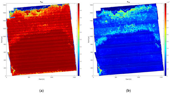
Figure 6.
TTS performance parameters obtained from processing of the SAS imagery. (a) pDC surface; (b) pFA surface.
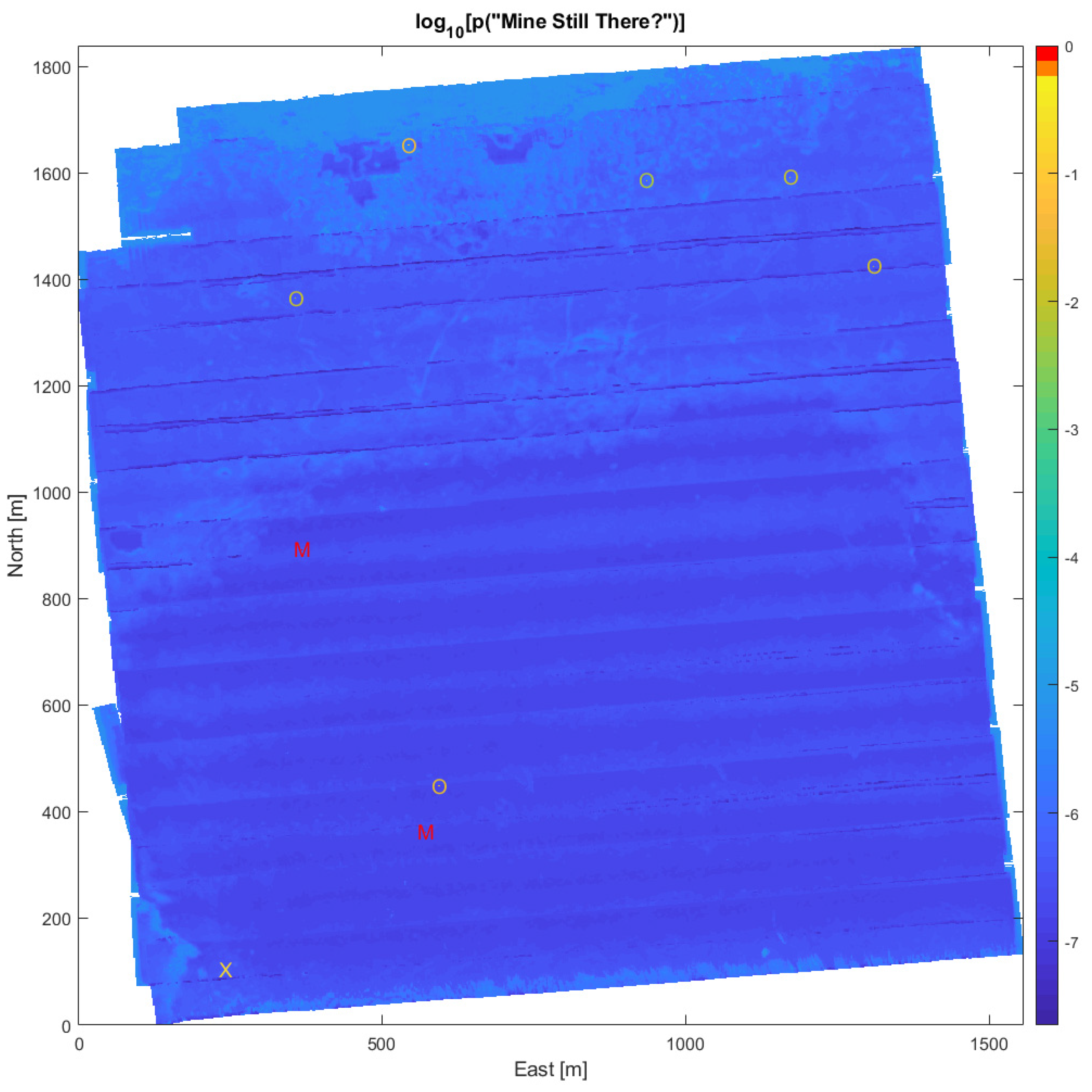
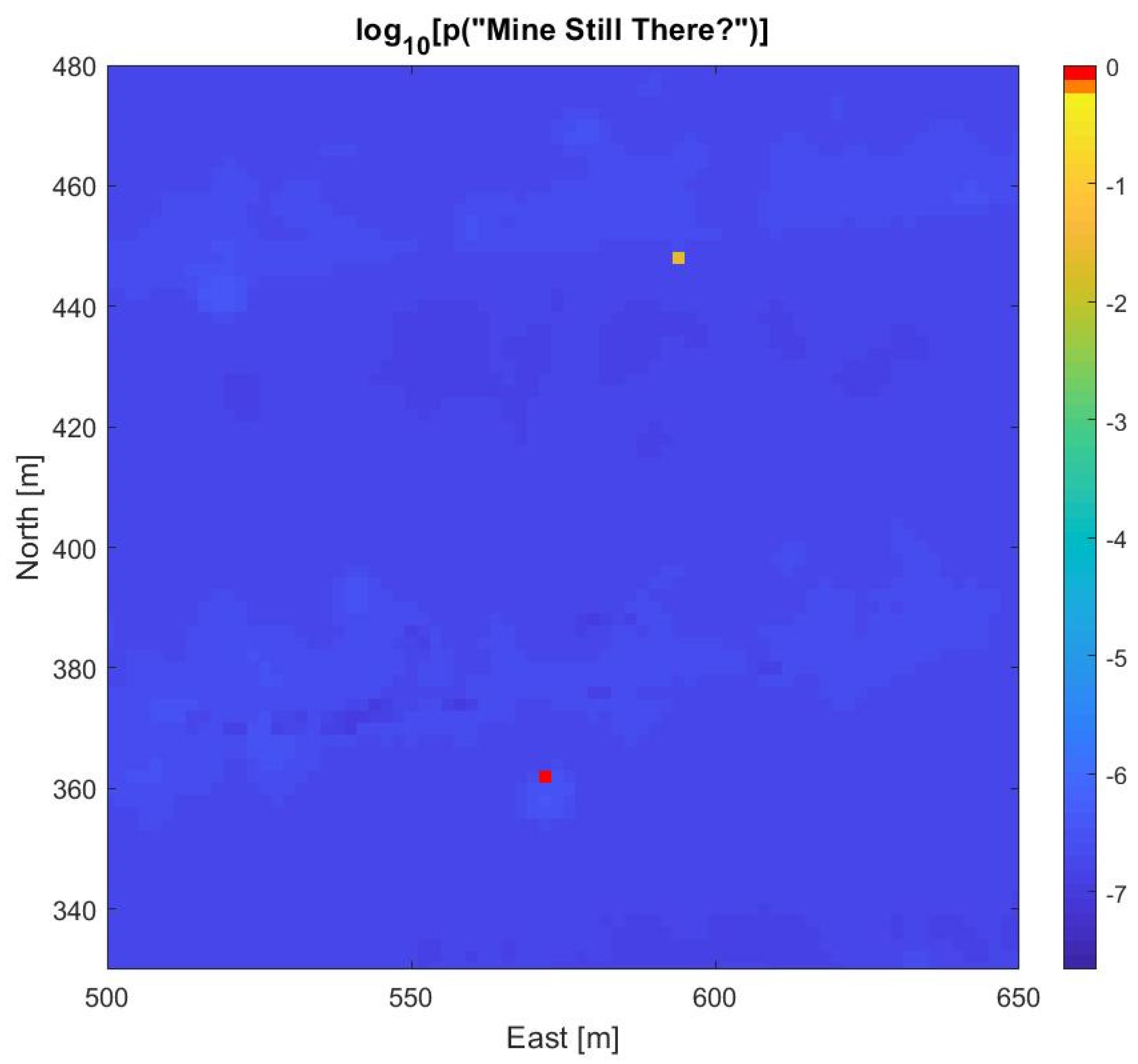
Manual analysis of the full-resolution SAS images (grid size 4 cm × 4 cm) from the survey yielded a list of nine MILCOs. The survey did not include optical identification of seafloor objects. In order to compute the marginal probability for the ‘Mine Still There?’ node of Figure 2, we have thus assumed that two of the MILCOs were identified as mines, six as NOMBOs, and the last MILCO was not identified. We further assume no neutralization was attempted. Figure 7 presents the resulting mine probability map from Bayesian evaluation. As individual cells are difficult to distinguish in the full map, the MILCO, NOMBO, and identified mine cells have been emphasized by distinct symbols (‘X’, ‘O’, ‘M’, respectively), which are color coded with the mine probability value of the cell. To visualize the relatively small variations in the background (non-MILCO cells), the color scale is logarithmic. The two cells with identified mines both achieve mine probability values above 90%, while the MILCO cell has a value of 18%. The six NOMBOs cells have probability values ranging from 0.5–2.8%, due to the geographical variations in pDC and pFA. Mine probability maps such as Figure 7 provide detailed information for planning further MCM efforts in the area, quantifying the risk for specific routes and thus selection of the safest route for follow-on traffic. Figure 8 shows a 150 m × 150 m section of the map in Figure 7, centered on two of the identified contacts. The symbols have been omitted because the individual cells are discernible in this zoom view.

Figure 7.
The mine probability surface (on a logarithmic scale) obtained by considering all the information in each cell. Symbols represent: identified mines (M), NOMBOs (O), and unidentified MILCOs (X). These symbols are also coloured by the logarithm of mine probability.

Figure 8.
A 150 m × 150 m zoom view of Figure 7, covering two of the identified contacts, which are visible as single cells with significantly higher mine probabilities than the background. The red cell corresponds to an identified mine (M) and the yellow cell to a NOMBO (O).
5. Discussion
The primary focus of this work is on estimating the number of mines remaining in a mine threat area through the fusion of performance estimates from the detection, classification, identification, and neutralization phases of mine hunting. The advancement in robotics, sensing, and perception has allowed for a change in the method by which MCM is evaluated, moving from a single probability [8] to a surface of probabilities that leverage high fidelity TTS performance estimates. These surfaces, such as the one demonstrated in Figure 7, represent the probability of a mine remaining in each geographical grid cell. While the concept of leveraging through the sensor performance and georeferenced performance grids has been presented previously in [5], this work employed embedded Bayesian networks to enable full process estimates that do not require the completion of each phase of MCM.
The ‘Bayes Net’ approach facilitates the incorporation of additional information from mine neutralization, including both initial observations (explosions) and the results of verification. This additional information has not previously been used in evaluation, and thus is not available to competing methods. The study presented here suggests the incorporation of this additional evidence improves performance at estimating the number of deployed mines (M). In this regard, the suggested method performed significantly better than the PESOS, Global Bayes and Global Bayes+ approaches.
An interesting observation from the representative network in Section 4.1 is that the explosion evidence is the main driver of this improvement. While the results of neutralization can be observed due to the sea surface expression of the neutralization, verification remains the best way to ensure that mines really are neutralized.
In comparing the estimation results, the PESOS method’s performance generally lagged the other methods, even though it performed comparably to the Bayes Nets up to the results in Figure 3. The technique used in PESOS to convert the posterior for pM into a posterior for M is likely the cause of the difference in performance.
The improved performance of the Bayes Net approach was robust to small changes in the weight placed on explosion evidence. The sensitivity analysis proposed in Section 3.3 examined the effects of modest changes to parameter eW, taking it from the actual value of 90% to 95% or 80%. Recall that eW is the probability that a neutralized mine will result in an explosion that is detected at the surface, provided such an explosion is watched for. The results showed little or no decline in relative estimation performance. Thus, the Bayes Net performance edge does not require perfect knowledge of explosion probabilities.
The Bayes Net approach might seem challenging to use because of the large number of parameters to set in Table 2; however, only the parameters above the line in that table make a difference in estimation. The parameters below the line can remain at default levels. Those parameters only matter in simulation, as they predict the decisions of human mine warfare officers. Estimation uses actual decisions not predicted ones, so these parameters simply have no effect on the probability computations (so long as they are not set to 0 or 1).
Another challenge for the Bayes Net approach is its long run time of nearly 30 min (as implemented with the sequential processing of grid cells on a mid-range personal computer). Without a significant improvement in speed, this amount of delay is certain to strain the patience of mine warfare officers, who are used to sub-second response times from their planning and evaluation support tools. Fortunately, parallel processing offers significant potential for speed improvements, depending on the number of computer cores available, because the Bayes Net approach treats grid cells independently. One might also replace Equation (1) with an analytic closed form solution that does not rely on Bayesian networks, but the computations involved are far from straightforward, as there are multiple paths of inference. Still, the Bayes Net approach is likely to be used only in situations where users have the option to wait for minutes for a more accurate result. Given that human lives are at stake, waiting a bit longer for results should often be worthwhile.
While this work provides the capability to use additional information in MCM evaluation, it currently only considers one mine type over one area. Typically, MCM risk evaluations will include multiple mine types, multiple segments, the environment, and critical features of the vessels transiting the area to compute a risk index. Further work will consider multiple mine types, as well as the evaluation of mine sweeping techniques. Through the application of these techniques, in combination with the advanced capabilities in sensing, perception, and robotics, high fidelity measurements make it possible to predict the probability of mines remaining more accurately, thereby improving measurements of follow-on risk, and allowing for the optimized application of further MCM resources.
Author Contributions
Conceptualization, T.R.H., W.A.C. and Ø.M.; methodology, T.R.H. and Ø.M.; software, T.R.H. and Ø.M.; validation, T.R.H., W.A.C. and Ø.M.; formal analysis, T.R.H.; resources, W.A.C. and Ø.M.; writing—original draft preparation, T.R.H.; writing—review and editing, T.R.H., W.A.C. and Ø.M.; visualization, T.R.H. and Ø.M.; supervision, W.A.C.; funding acquisition, W.A.C. and Ø.M. All authors have read and agreed to the published version of the manuscript.
Funding
This work was funded by the Royal Norwegian Navy, as well as by Defence Research and Development Canada project 01cb on Naval Mine Countermeasures.
Data Availability Statement
Restrictions apply to the availability of the data used in Section 4.3.
Acknowledgments
The authors thank Sarah Tierney for her artistic contributions to the graphical abstract.
Conflicts of Interest
The authors declare no conflict of interest. The funders had no role in the design of the study; in the collection, analyses, or interpretation of data; in the writing of the manuscript, or in the decision to publish the results.
Appendix A
The details of how to specify conditional probability tables for the DAG in Figure 2, based on the parameters given in Table 2, are given here in Figure A1, Figure A2 and Figure A3.
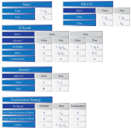
Figure A1.
A selection of conditional probability tables for the Bayesian network that will be used to model inference within each grid cell. The top of each table gives the variable name. Cells in dark blue identify variables on which the table depends. These dependencies are the nodes from which arrows are incoming to the named variable. Each table defines a probability for each possible configuration of states for these dependencies.


Figure A2.
A selection of conditional probability tables for the Bayesian network that will be used to model inference within each grid cell. The tables for the ‘Remaining Mine?’ and ‘Detect Explosion?’ variables are defined using Boolean expressions (as indicated by a triangle symbol). The if expression has three parts: a condition, a sub-expression for when the condition is True, and a second sub-expression for when the condition is False.
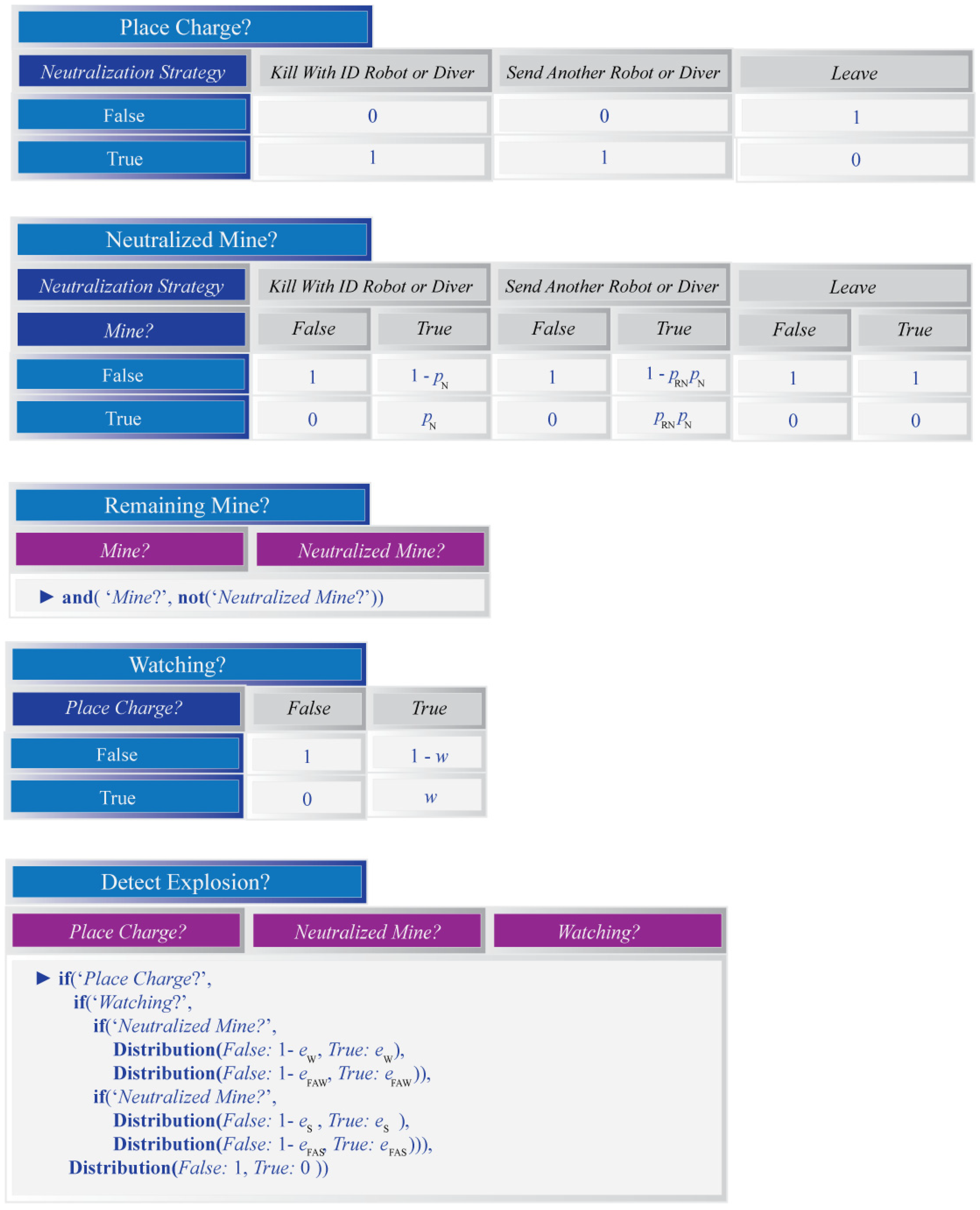
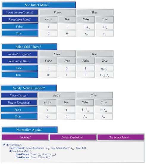
Figure A3.
The last set of conditional probability tables for the Bayesian network that will be used to model inference within each grid cell. The table for the ‘Neutralize Again?’ variable is defined using Hugin’s NoisyOR, if and Distribution expressions. More information on these may be found in the Hugin documentation.

References
- Navy Department. 21st Century U.S. Navy Mine Warfare: Ensuring Global Access and Commerce; U.S. Department of the Navy, Program Executive Office for Littoral and Mine Warfare: Washington, DC, USA, 2009; Volume 31.
- Hagen, P.E.; Størkersen, N.; Marthinsen, B.E.; Sten, G.; Vestgård, K. Military operations with HUGIN AUVs: Lessons learned and the way ahead. In Proceedings of the IEEE Oceans Europe Conference, Brest, France, 20–23 June 2005. [Google Scholar]
- Midtgaard, Ø.; Alm, I.; Sæbø, T.O.; Geilhufe, M.; Hansen, R.E. Performance assessment tool for AUV based mine hunting. In Proceedings of the Institute of Acoustics, Lerici, Italy, 16–19 November 2014; Volume 36, pp. 120–129. [Google Scholar]
- Wiig, M.S.; Krogstad, T.R.; Midtgaard, Ø. Autonomous identification planning for mine countermeasures. In Proceedings of the IEEE/OES AUV Conference, Southampton, UK, 24–27 September 2012. [Google Scholar] [CrossRef]
- Midtgaard, Ø.; Warakagoda, N.; Davies, G.; Connors, W.; Geilhufe, M. Multi-phase performance evaluation for modern minehunting systems. In Proceedings of the SPIE, Baltimore, ML, USA, 15–17 April 2019. [Google Scholar] [CrossRef]
- Strenzke, R.; Strode, C. A Bayesian information fusion approach to naval mine-hunting system of systems operation planning and evaluation. In Proceedings of the UACE 2019 Conference, Hersonissos, Greece, 30 June–5 July 2019; pp. 817–824. [Google Scholar]
- Babel, L.; Zimmermann, T. Planning safe navigation routes through mined waters. Eur. J. Oper. Res. 2015, 241, 99–108. [Google Scholar] [CrossRef]
- Bryan, K. Algorithms for Decision Aid for Risk Evaluation (DARE) Version 2.1; NURC-FR-2006-002; NATO STO CMRE: La Spezia, Italy, 2006. [Google Scholar]
- Percival, A.M.; Couillard, M.; Midtgaard, Ø.; Fox, W. Unmanned Systems, Autonomy and Side-Looking Sonar: A Framework for Integrating Contemporary Systems into the Operational Architecture; CMRE-FR-2013-013; NATO STO CMRE: La Spezia, Italy, 2013. [Google Scholar]
- Myers, V.; Davies, G.; Petillot, Y.; Reed, S. Planning and evaluation of AUV missions using data-driven approaches. In Proceedings of the MINWARA Conference, Monterey, CA, USA, 22–24 May 2006. [Google Scholar]
- Reed, S.; Petillot, Y.; Cormack, A. PATT: A performance analysis and training tool for the assessment and adaptive planning of mine counter measures (MCM) operations. In Proceedings of the Institute of Acoustics, Edinburgh, UK, 17–18 October 2007. [Google Scholar]
- Gazagnaire, J.; Beaujean, P.; Stack, J. Combining model-based and in situ performance prediction to evaluate detection & classification performance. In Proceedings of the Institute of Acoustics, Edinburgh, UK, 17–18 October 2007. [Google Scholar]
- Johnson, S.; Low-Choy, S.; Mengersen, K. Integrating Bayesian networks and Geographic Information Systems: Good practice examples. Integr. Environ. Assess. Manag. 2011, 8, 473–479. [Google Scholar] [CrossRef] [PubMed]
- Bolouki, S.; Ramazi, H.; Maghsoudi, A.; Pour, A.; Sohrabi, G. A remote sensing-based application of Bayesian networks for epithermal gold potential mapping in Ahar-Arasbaran Area, NW Iran. Remote Sens. 2019, 12, 105. [Google Scholar] [CrossRef] [Green Version]
- Terefenko, P.; Paprotny, D.; Giza, A.; Morales-Nápoles, O.; Kubicki, A.; Walczakiewicz, S. Monitoring cliff erosion with LiDAR surveys and Bayesian network-based data analysis. Remote Sens. 2019, 11, 843. [Google Scholar] [CrossRef] [Green Version]
- Li, Y.; Martinis, S.; Wieland, M.; Schlaffer, S.; Natsuaki, R. Urban flood mapping using SAR intensity and interferometric coherence via Bayesian network fusion. Remote Sens. 2019, 11, 2231. [Google Scholar] [CrossRef] [Green Version]
- Moe, S.J.; Carriger, J.F.; Glendell, M. Increased use of Bayesian network models has improved environmental risk assessments. Integr. Environ. Assess. Manag. 2020, 17, 53–61. [Google Scholar] [CrossRef] [PubMed]
- Dlamini, W.M. Application of Bayesian networks for fire risk mapping using GIS and remote sensing data. GeoJournal 2011, 76, 283–296. [Google Scholar] [CrossRef]
- Kaikkonen, L.; Parviainen, T.; Rahikainen, M.; Uusitalo, L.; Lehikoinen, A. Bayesian networks in environmental risk assessment: A review. Integr. Environ. Assess. Manag. 2021, 17, 62–78. [Google Scholar] [CrossRef] [PubMed]
- Oliveira Silva, A.C. A Spatio-Temporal Bayesian Network Model: A Case Study in Brazilian Amazon Deforestation Prediction. Ph.D. Thesis, Instituto Nacional de Pesquisas Espaciais, São José dos Campos, Brazil, 4 May 2020. [Google Scholar]
- Fenton, N.; Neil, M. Risk Assessment and Decision Analysis with Bayesian Networks; CRC Press: Boca Raton, FL, USA, 2012. [Google Scholar]
- Jensen, F.V. An Introduction to Bayesian Networks; UCL Press: London, UK, 1996. [Google Scholar]
- Madsen, A.L.; Jensen, F.V.; Kjaerulff, U.B.; Lang, M. The HUGIN tool for probabilistic graphical models. Int. J. Artif. Int. Tools 2005, 14, 507–543. [Google Scholar] [CrossRef]
- Madsen, A.L.; Jensen, F.V.; Salmerón, A.; Langseth, H.; Nielsen, T.D. A parallel algorithm for Bayesian network structure learning from large data sets. Knowl. Based Syst. 2017, 117, 46–55. [Google Scholar] [CrossRef] [Green Version]
- Hansen, R.E.; Callow, H.J.; Sæbø, T.O.; Synnes, S.A.V. Challenges in Seafloor Imaging and Mapping with Synthetic Aperture Sonar. IEEE Trans. Geosci. Remote Sens. 2011, 49, 3677–3687. [Google Scholar] [CrossRef]

Publisher’s Note: MDPI stays neutral with regard to jurisdictional claims in published maps and institutional affiliations. |
© 2021 by the authors. Licensee MDPI, Basel, Switzerland. This article is an open access article distributed under the terms and conditions of the Creative Commons Attribution (CC BY) license (https://creativecommons.org/licenses/by/4.0/).