Multipath Exploitation with Time Reversal Waveform Covariance Matrix for SNR Maximization

Abstract

Radar target detection has a wide range of applications in the military and civilian remote sensing fields; in particular, the target detection in multipath environments has attracted many scholars’ attention in recent years. The abundant multipath signals severely interfere with the detection performance and accuracy of parameter estimation of traditional algorithms. Under Gaussian white noise environments, this letter proposes an adaptive time reversal (TR) waveform covariance matrix (WCM) design method with multipath exploitation to improve the maximum signal-to-noise ratio (SNR) at the receiver in multipath environments. This equivalently improves the detection probability. The proposed two-stage algorithm firstly adapts the time-reversal echo to construct a multipath information matrix with a Hermitian structure. Secondly, the letter transforms the maximized SNR problem into semidefinite programming (SDP), which is constrained by a constant total transmit power. Consequently, the waveform covariance matrix is obtained by solving semidefinite programming. Simulation experiments verify the adaptability and effectiveness of the proposed algorithm.

1. Introduction

Multipath is a common phenomenon in radar applications, which is usually caused by the reflection and refraction of objects in the process of electromagnetic wave propagation [1,2]. It is common in urban environments and low-angle tracking (such as sea surface) scenes. In multipath environments, radar-received signals include not only the line-of-sight signal, but also contain specular reflection and various diffuse multipath signals. These multipath signals are correlated with the line-of-sight signal and interfere with the line-of-sight signal in the space, time, and Doppler domains, which leads to the performance degradation of classical algorithms [3]. There are two main approaches to deal with multipath signals. One is suppressing multipath as much as possible, which needs the prior information of multipath. Once the multipath information is unknown or inaccurately known, algorithms’ performance degrades significantly. Oppositely, another way is utilizing multipath. As a representative of the latter, time reversal (TR) takes advantage of the reciprocity of wave propagation in a time-invariant medium, which achieves the space-time focusing effect of the signal at the target by time reversing, normalizing the energy, and transmitting again [4]. Therefore, time reversal is widely used in array signal processing [5,6,7].

Unlike traditional phased array radars that transmit a single waveform, multiple-input multiple-output (MIMO) radar allows each transmitting element to emit different waveforms [8]. With the additional degrees of freedom provided by the diversity of waveforms, MIMO radar system performance is also improved. Therefore, MIMO radar waveform design is the focus of many scholars. At present, MIMO radar waveform design approaches can be divided into two categories. One is to design the waveform signal transmitted by each element directly [9], and the other is first to develop the transmit waveform covariance matrix (WCM) and then design the corresponding waveform according to the designed waveform covariance matrix [10,11].

The waveform design aiming for multipath is essentially to design a corresponding waveform that suitable for the signal-dependent scenes. In the existence of signal-dependent signals, one is to develop the corresponding waveform based on the prior knowledge of the target and interference. Chen proposes an iterative algorithm to improve the performance of target detection by utilizing the statistics of a target impulse response [12]. Aashish Sharma minimizes multipath interference through the constant of constant power and/or useful pulse compression features [13]. When it comes to design the waveform with multipath exploitation, B. Chakraborty selects the parameters of the transmitted waveform dynamically to minimize the predicted mean-squared tracking error in urban specular reflection environments [14]. However, this algorithm ignores the diffuse multipath, so its applicability under diffuse multipath environments is still to be studied. Whether suppressing multipath or exploiting multipath, a priori knowledge about multipath is required. Moreover, traditional methods are difficult to accurately estimate the number of multipath and the corresponding direction of arrival due to diffuse multipath’s randomness and uncertainty, which makes related waveform design difficult.

To solve the waveform design difficulties in multipath environments, this letter puts forward an adaptive TR waveform design algorithm with multipath exploitation. The proposed two-stage algorithm first obtains the Toeplitz matrix with multipath information. Then, it generates the WCM by maximizing the SNR under the constraint of constant total transmit power.

The arrangement of this letter is organized as follows: Section 2 formulates the multipath system model; Section 3 derives the adaptive WCM design algorithm; Section 4 presents the simulation results; Section 5 concludes the letter.

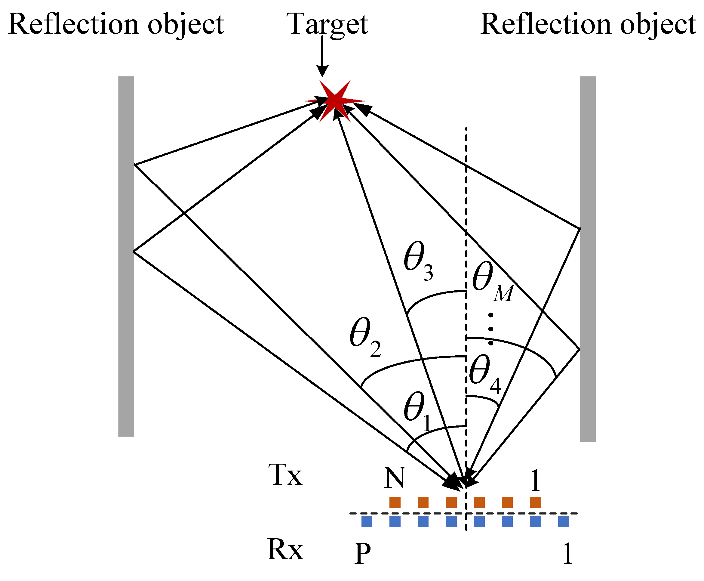
2. Multipath System Model

2.1. MIMO Radar

As shown in Figure 1, consider a monostatic MIMO radar consists of two colocated arrays. They are equipped with N elements and P elements at the transmitter and the receiver, respectively. For each array, the element inner distance is half a wavelength. There exists only one interesting target and M pieces of paths. The transmission paths include one direct path and $M-1$ reflection paths. As for i-th path, the attenuation factor, delay of time, and direction of arrival (DOA) are ${\alpha }_i$, ${\tau }_i$, ${\theta }_i$ respectively. It is worth mentioning that, due to the randomness of diffuse multipath, the number of multipath is unknown in reality.

The first probing signal emitted by each transmit element is $f_n\left(t\right)e^{j2\pi f_{c}t}(1\le n\le N)$, where $f_c$ is the carrier frequency, $f_n\left(t\right)$ is the baseband envelope of the probing signal. All N transmitting signal can be written in the vector form:$\mathit{f}={[f_1,f_2,\dots ,f_N]}^T$. Suppose that the baseband signal is orthogonal to each other, that is, $\mathit{f}{\mathit{f}}^H={\mathit{f}}^{*}{\mathit{f}}^T={\mathbf{I}}_N$, where ${\mathbf{I}}_N$ is an identity matrix. For static targets or slow-moving targets, the Doppler shift can be ignored. Thus, the receiving signal of p-th $(1\le p\le P)$ element is [15]:

$$\begin{array}{cc}\hfill r_p\left(t\right)& =\sum _{m_b=1}^M\sum _{m_f=1}^M\sum _{n=1}^N\stackrel{{\alpha }_l}{\overbrace{{\alpha }_{m_f}{\alpha }_{m_b}}}{f}_n(t-{\tau }_{n{m}_f}\left(t\right)-{\tau }_{p{m}_b}\left(t\right))\times e^{j{\omega }_c(t-{\tau }_{n{m}_f}\left(t\right)-{\tau }_{p{m}_b}\left(t\right))}+n_p\left(t\right),\hfill \end{array}$$

(1)

where $m_b$ and $m_f$ represent the backward scattering path and forward scattering path, $l=(m_f,m_b)$ represents a round trip. ${\tau }_{n{m}_f}$ and ${\tau }_{p{m}_b}$ are the propagation delays via forward and backward multipath between the n-th transmit element to the target and from the target to the p-th receive element, respectively. In the vector form, $\mathit{r}={[r_1,r_2,\dots ,r_P]}^T$ is recorded as:

$$\begin{array}{c}\hfill \mathit{r}\left(t\right)=\sum _{l=1}^L\stackrel{{\tilde{\alpha }}_l}{\overbrace{{\alpha }_l{e}^{-j{\omega }_c{\tau }_l\left(0\right)}}}\mathbf{A}\left({\Theta }_l\right)\mathit{f}(t-{\tau }_l\left(0\right))+\mathbf{n}\left(t\right),\end{array}$$

(2)

where the carrier angular frequency ${\omega }_c=2\pi f_c$, ${\tau }_l\left(0\right)={\tau }_{1m_f}\left(0\right)+{\tau }_{1m_b}\left(0\right)$ is the delay between the reference transmit and receive element (1,1), $\mathbf{n}\left(t\right)$ is the Gaussian white noise. $\mathbf{A}\left({\Theta }_l\right)={\mathit{\alpha }}_R\left({\theta }_{m_b}\right){\mathit{\alpha }}_T^T\left({\theta }_{m_f}\right)$ is the transmit-receive steering matrix, where ${\mathit{\alpha }}_R$ and ${\mathit{\alpha }}_T$ are given by:

$$\begin{array}{c}\hfill {\mathit{\alpha }}_R\left({\theta }_{m_b}\right)={[1,e^{-j{\omega }_c{\tau }_1^T\left({\theta }_{m_b}\right)},\dots ,e^{-j{\omega }_c{\tau }_N^T\left({\theta }_{m_b}\right)}]}^T,\end{array}$$

(3)

$$\begin{array}{c}\hfill {\mathit{\alpha }}_T\left({\theta }_{m_f}\right)={[1,e^{-j{\omega }_c{\tau }_1^T\left({\theta }_{m_f}\right)},\dots ,e^{-j{\omega }_c{\tau }_P^T\left({\theta }_{m_f}\right)}]}^T.\end{array}$$

(4)

2.2. TR MIMO Radar

According to the principle of TR, $\mathit{r}\left(t\right)$ is time-reversed, conjugated, energy normalized by c and retransmitted. The second transmitting signal is $c{\mathit{r}}^{*}(-t)$, where ${(·)}^{*}$ represents the conjugation operator. The normalization coefficient c is:

$$\begin{array}{c}\hfill c=\sqrt{{\left|\right|\mathit{f}\left|\right|}_F/{\left|\right|\mathit{r}\left|\right|}_F},\end{array}$$

(5)

where $\left|\right|·{\left|\right|}_F$ repersents the Frobenius norm.

Following the derivation of (2), the TR receiving signal $\mathbf{x}\left(t\right)$ can be written as:

$$\begin{array}{cc}\mathbf{x}\left(t\right)\hfill & =c{\displaystyle \sum _{l^{\prime }=1}^L}{\tilde{\alpha }}_{l^{\prime }}{\mathbf{A}}^T({\mathbf{\Theta }}_{l^{\prime }}){\mathit{r}}^{*}(-t+{\tau }_{l^{\prime }}(0))+\mathbf{v}(t)\hfill \\ & \approx c{\displaystyle \sum _{l=1}^L}{\left|{\tilde{\alpha }}_{f^{\prime }}\right|}^2\stackrel{{\mathbf{A}}_{\mathrm{TR}}({\mathbf{\Theta }}_l)}{\overbrace{{\mathbf{A}}^T({\mathbf{\Theta }}_l){\mathbf{A}}^{*}({\mathbf{\Theta }}_l)}}{\mathit{f}}^{*}(-t)+\stackrel{\mathbf{u}(t)}{\overbrace{c{\displaystyle \sum _{l^{\prime }=1}^L}{\tilde{\alpha }}_{l^{\prime }}{\mathbf{A}}^T{\mathit{n}}^{*}(-\mathit{t})+\mathbf{v}(t),}}\hfill \end{array}$$

(6)

where $\mathbf{v}\left(t\right)$ is the observation noise with the convariance ${\sigma }_n^2{\mathit{I}}_{\mathit{P}}$ for the TR stage, $\mathbf{u}\left(t\right)$ is the accumulated noise, which takes $\mathbf{n}\left(t\right)$ and $\mathbf{v}\left(t\right)$ into account. Similar to reference [16], $\mathbf{u}\left(t\right)$ is approximated as white noise. In line with the super-resolution focusing property of TR [17], the approximation in (6) is valid.

Taking the l-th round trip as an example, the matrix ${\mathbf{A}}_{\mathrm{TR}}\left({\Theta }_l\right)$ can be written as:

$$\begin{array}{cc}\hfill {\mathbf{A}}_{\mathrm{TR}}\left({\mathbf{\Theta }}_l\right)& ={\mathbf{A}}^T\left({\mathbf{\Theta }}_l\right){\mathbf{A}}^{*}\left({\mathbf{\Theta }}_l\right)\hfill \\ \hfill & ={\left({\mathit{\alpha }}_R\left({\theta }_{m_b}\right){\mathit{\alpha }}_T^T\left({\theta }_{m_f}\right)\right)}^T{\left({\mathit{\alpha }}_R\left({\theta }_{m_b}\right){\mathit{\alpha }}_T^T\left({\theta }_{m_f}\right)\right)}^{*}\hfill \\ \hfill & =P{\mathit{\alpha }}_T\left({\theta }_{m_f}\right){\mathit{\alpha }}_T^H\left({\theta }_{m_f}\right),\hfill \end{array}$$

(7)

where ${(·)}^H$ is the conjugate transpose operator, and the matrix ${\mathbf{A}}_{\mathrm{TR}}$ is related to the forward scattering angle for one round trip. According to this characteristic, the $\mathbf{x}\left(t\right)$ in (6) can be rewritten as:

$$\begin{array}{cc}\hfill \mathbf{x}\left(t\right)& =c{c}_1\sum _{m_f=1}^M{\left|{\tilde{\alpha }}_{m_f}\right|}^2{\mathit{\alpha }}_T\left({\theta }_{m_f}\right){\mathit{\alpha }}_T^H\left({\theta }_{m_f}\right){\mathit{f}}^{*}(-t)+\mathbf{u}\left(t\right)\hfill \\ \hfill & =c{c}_1{\mathbf{A}}_{\mathbf{M}}diag\left(\mathit{\eta }\right){\mathbf{A}}_{\mathbf{M}}^H{\mathit{f}}^{*}(-t)+\mathbf{u}\left(t\right),\hfill \end{array}$$

(8)

where ${\mathbf{A}}_{\mathbf{M}}=[{\mathit{\alpha }}_T\left({\theta }_{m_{f_1}}\right),{\mathit{\alpha }}_T\left({\theta }_{m_{f_2}}\right),\dots ,{\mathit{\alpha }}_T\left({\theta }_{m_{f_M}}\right)]$, $diag$($\mathit{\eta }$) is a diagonal matrix, whose diagonal element is $\mathit{\eta }$ and others are zero. $\mathit{\eta }=[{|{\tilde{\alpha }}_{m_{f_1}}|}^2,\dots ,{|{\tilde{\alpha }}_{m_{f_M}}|}^2],{\tilde{\alpha }}_{m_{f_i}}={\alpha }_{m_{f_i}}{e}^{-j{\omega }_c{\tau }_{1m_{f_i}}\left(0\right)}(1\le i\le M)$ and $c_1=P\left({\sum }_{m_b^{{}^{\prime }}=1}^M{\left|{\tilde{\alpha }}_{m_b^{{}^{\prime }}}\right|}^2\right)$.

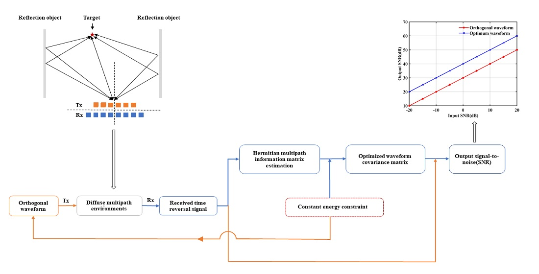
3. The Proposed Two-Stage Algorithm

This section formulates the proposed algorithm from two steps. First, the letter obtains the multipath information matrix from TR observation in (8). After having the multipath information matrix, we derive the expression of the output SNR and design the corresponding waveform covariance matrix under the constraint of total transmit power.

3.1. Hermitian Multipath Information Matrix Reconstruction

Let $\mathit{T}=c_1{\mathbf{A}}_{\mathbf{M}}diag\left(\mathit{\eta }\right){\mathbf{A}}_{\mathbf{M}}^H$ represent the multipath information matrix, and the corresponding estimator is $\widehat{\mathit{T}}$. Since $c_1$ is a real value, the elements of $\mathit{\eta }$ also are real values, $\mathit{T}$ holds the characteristic of Hermitian. What’s more, $\mathit{T}$ has the structure of a covariance matrix, so it is positive semidefinite. To obtain the matrix $\widehat{\mathit{T}}$, we introduce the following SDP problem using (8):

$$\begin{array}{cc}\hfill \underset{\widehat{\mathit{T}}}{min}& \left|\right|\mathbf{x}\left(t\right)-c\widehat{\mathit{T}}{\mathit{f}}^{*}(-t){\left|\right|}_F^2\hfill \\ \hfill s.t.& \widehat{\mathit{T}}={\widehat{\mathit{T}}}^H,\widehat{\mathit{T}}⪰0,\hfill \end{array}$$

(9)

where $\widehat{\mathit{T}}={\widehat{\mathit{T}}}^H$ shows that $\mathit{T}$ is a Hermitian matrix, ⪰ represents the positive semidefinite.

3.2. Waveform Covariance Matrix Design

In this section, we keep the energy coefficient c as a constant value for different waveforms to only show the waveform’s effect, and we omit it in the following expressions. Denote the optimum transmit waveform as $\mathit{g}\left(t\right)$, similiar to (8), we can obtain the corresponding TR echo $\mathit{z}\left(t\right)$:

$$\begin{array}{cc}\hfill \mathbf{z}\left(t\right)& =c_1\sum _{m_f=1}^M{\left|{\tilde{\alpha }}_{m_f}\right|}^2{\mathit{\alpha }}_T\left({\theta }_{m_f}\right){\mathit{\alpha }}_T^H\left({\theta }_{m_f}\right){\mathit{g}}^{*}(-t)+\mathbf{w}\left(t\right)\hfill \\ \hfill & =c_1{\mathbf{A}}_{\mathbf{M}}diag\left(\mathit{\eta }\right){{\mathbf{A}}_{\mathbf{M}}}^H{\mathit{g}}^{*}(-t)+\mathbf{w}\left(t\right),\hfill \end{array}$$

(10)

where $\mathbf{w}\left(t\right)$ is the noise matrix and ${\sigma }_n^2$ is its corresponding noise power.

According to (10), the SNR at the receiver can be describe as:

$$\begin{array}{cc}\hfill \mathrm{SNR}& =\frac{tr((c_1{\sum }_{m_f=1}^M|{\tilde{\alpha }}_{m_f}{|}^2{\mathit{\alpha }}_T({\theta }_{m_f}){\mathit{\alpha }}_T^H({\theta }_{m_f}){\mathit{g}}^{*}(-t))(c_1{\sum }_{m_f^{{}^{\prime }}=1}^M|{\tilde{\alpha }}_{m_f^{{}^{\prime }}}{|}^2{\mathit{\alpha }}_T({\theta }_{m_f^{{}^{\prime }}}){\mathit{\alpha }}_T^H({\theta }_{m_f^{{}^{\prime }}}){\mathit{g}}^{*}(-t){)}^H)}{{\sigma }_n^2}\hfill \\ \hfill & =\frac{tr(c_1^2{\sum }_{m_f=1}^M{\sum }_{m_f^{{}^{\prime }}=1}^M|{\tilde{\alpha }}_{m_f}{|}^2(|{\tilde{\alpha }}_{m_f^{{}^{\prime }}}{|}^2{)}^H{\mathit{\alpha }}_T({\theta }_{m_f}){\mathit{\alpha }}_T{({\theta }_{m_f})}^H\mathit{R}{\mathit{\alpha }}_T({\theta }_{m_f^{{}^{\prime }}}){\mathit{\alpha }}_T{({\theta }_{m_f^{{}^{\prime }}})}^H)}{{\sigma }_n^2},\hfill \end{array}$$

(11)

where $tr(·)$ is the matrix trace operator, $\mathit{R}$ is the covariance matrix of the input signal ${\mathit{g}}^{*}(-t)$.

To maximize the SNR in (11), it is equivalent to maximizing the following criterion:

$$\begin{array}{c}\hfill tr(c_1^2\sum _{m_f=1}^M\sum _{m_f^{{}^{\prime }}=1}^M|{\tilde{\alpha }}_{m_f}{|}^2(|{\tilde{\alpha }}_{m_f^{{}^{\prime }}}{|}^2{)}^H{\mathit{\alpha }}_T({\theta }_{m_f}){\mathit{\alpha }}_T{({\theta }_{m_f})}^H\mathit{R}{\mathit{\alpha }}_T({\theta }_{m_f^{{}^{\prime }}}){\mathit{\alpha }}_T{({\theta }_{m_f^{{}^{\prime }}})}^H)=tr(\mathit{R}\mathit{B}),\end{array}$$

(12)

where $\mathit{B}=c_1^2{\sum }_{m_f=1}^M{\sum }_{m_f^{{}^{\prime }}=1}^M|{\tilde{\alpha }}_{m_f}{|}^2\left(\right|{\tilde{\alpha }}_{m_f^{{}^{\prime }}}{{|}^2)}^H{\mathit{\alpha }}_T\left({\theta }_{m_f^{{}^{\prime }}}\right){\mathit{\alpha }}_T{\left({\theta }_{m_f^{{}^{\prime }}}\right)}^H{\mathit{\alpha }}_T\left({\theta }_{m_f}\right){\mathit{\alpha }}_T{\left({\theta }_{m_f}\right)}^H$.

Notice that $\mathit{B}=\mathit{T}{\mathit{T}}^H$, after having the eatimator of $\mathit{T}$ from (9), we can replace $\mathit{B}$ by the corresponding estimator $\widehat{\mathit{B}}=\widehat{\mathit{T}}{\widehat{\mathit{T}}}^H$. Then, the SNR maximizion in (12) can be formulated as the following semidefinite program [18]:

$$\begin{array}{cc}\hfill \underset{\mathit{R}}{max}& tr\left(\mathit{R}\widehat{\mathit{B}}\right)\hfill \\ \hfill s.t.& tr\left(\mathit{R}\right)=P_0,\mathit{R}⪰0,\hfill \end{array}$$

(13)

where $P_0=tr\left({\mathit{f}}^{*}{\left({\mathit{f}}^{*}\right)}^H\right)$ is the constant total transmit power. The constraint $\mathit{R}⪰0$ suggests that $\mathit{R}$ is a positive semidefinite matrix.

Applying the inequality in matrix theory, $tr\left(\mathit{R}\widehat{\mathit{B}}\right)\le tr\left(\mathit{R}\right){\lambda }_{max}\left(\widehat{\mathit{B}}\right)=P_0{\lambda }_{max}\left(\widehat{\mathit{B}}\right)$, where ${\lambda }_{max}\left(\widehat{\mathit{B}}\right)$ is the maximum eigenvalue of $\widehat{\mathit{B}}$. Finally, the designed waveform covariance matrix $\mathit{R}$ is:

$$\mathit{R}=P_0\mathit{u}{\mathit{u}}^H,$$

(14)

where $\mathit{u}$ is the eigenvector of $\widehat{\mathit{B}}$, which corresponds to the maximum eigenvalue of $\widehat{\mathit{B}}$.

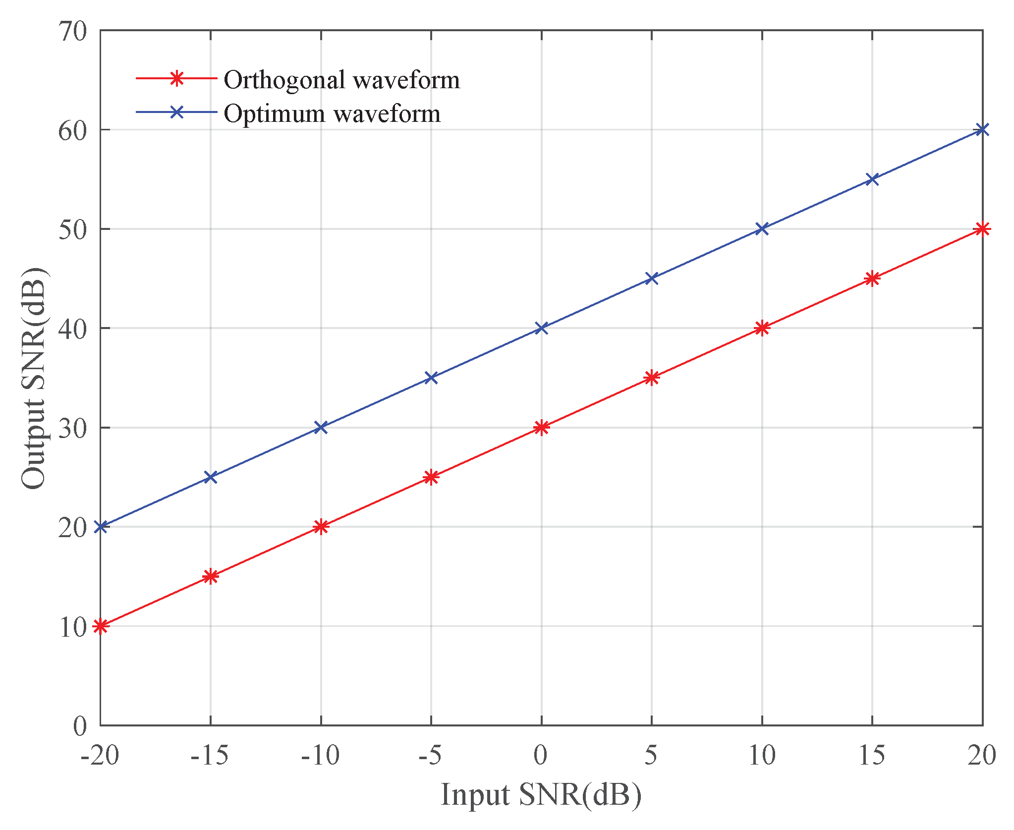
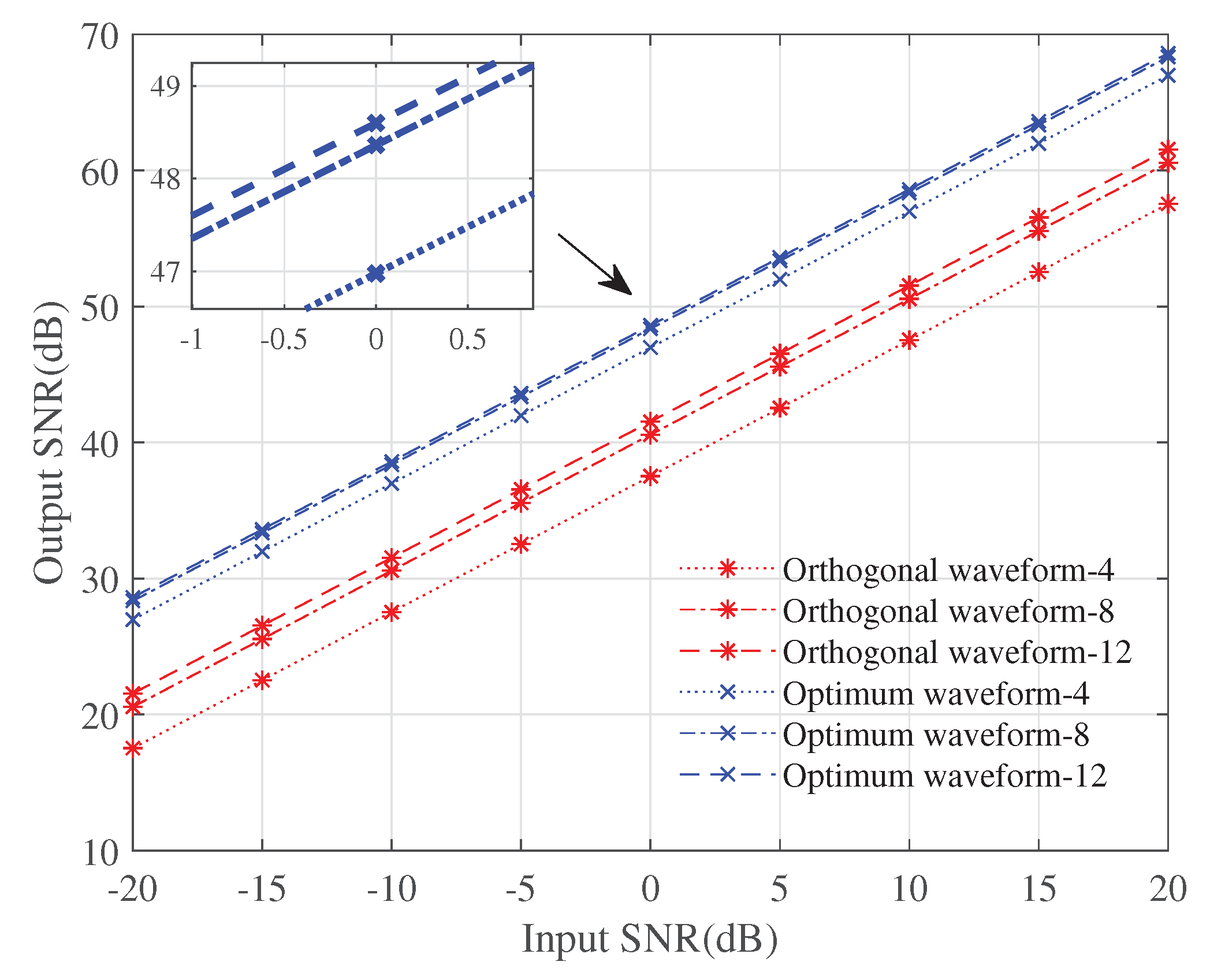
4. Simulation Results

This section verifies the effectiveness of the proposed algorithm in terms of the output SNR at the receiver under two situations: (a) transmitting orthogonal waveform (b) transmitting the optimum waveform of the proposed algorithm. Specifically, the letter examines the effectiveness from three aspects: (1) output SNR versus the input SNR (The input SNR is defined as $10lo{g}_{10}\left(\frac{P_0}{{\sigma }_n^2}\right)$); (2) output SNR with different numbers of multipath; (3) output SNR with different multipath amplitudes at a fixed input SNR. The basic parameters in experiments are as follows: array elements number $N=P=10$, carrier frequency $f_c=200$ MHz, and the snapshots are 256.

4.1. Output SNR Versus Input SNR

The first experiment verifies the validity of the proposed algorithm in a diffuse multipath environment. Suppose the path number $M=4$, the DOAs of each path are 2°, −2°, 10°, −16°, and corresponding delays and attenuation factors are randomly set as $0ns,2ns,4ns,12ns$ and $1.0000+0.0000i,0.9319+0.2520i,0.8375+0.2830i,0.2255-0.4586i$, respectively. The input SNR varies from $-20$ dB to 20 dB with an interval of 5 dB. We conduct 100 Monte Carlo trials at each input SNR and select the average output SNR of all Monte Carlo simulations as the final output SNR.

As shown in Figure 2, the optimum waveform, which matches the multipath environments, increases the output SNR of 10 dB by comparing it with the orthogonal waveform. This gain remains stable around the whole input SNR. The result shows that the proposed waveform covariance matrix is superior in multipath environments.

4.2. Output SNR with Different Numbers of Multipath

This experiment verifies the influence of different numbers of multipath on the output SNR. The multipath’s parameters are recorded in

Table 1. Parameters of multipath.

Path Number	DOA (°)	Amplitude Factor	Delay Time (ns)
1	2	1.0000 + 0.0000i	0
2	−2	0.8438 − 0.0753i	2.0
3	−5.4	0.6119 − 0.5846i	6.1
4	5.5	0.8213 + 0.0168i	10.3
5	−6.8	0.7945 − 0.0884i	17.5
6	9.4	0.4334 − 0.6536i	20.4
7	−10.2	0.7189 − 0.1566i	31.2
8	11.2	0.5467 − 0.4211i	34.7
9	−11.6	0.5111 − 0.3501i	35.4
10	12.8	0.5661 + 0.1740i	39.0
11	−14	0.4288 − 0.3190i	40.6
12	19.5	0.4773 − 0.1480i	45.9

. We simulate three groups of multipath for comparison and the numbers of multipath are 4, 8, and 12, respectively. Group 1 includes the former four pieces of multipath in Table 1, while group 2 and group 3 containing the former eight and all the pieces of multipath, respectively. As for all the groups, the input SNR changes uniformly from −20 dB to 20 dB with an interval of 5 dB each time. The final output SNR is calculated by averaging the output SNR of 100 Monte Carlo trails.

In Figure 3, the label “Optimum waveform-4” means the number of multipath $M=4$, and the transmit waveform is the optimum waveform (other labels are similar). With the increase of the number of multipath, the output SNR improves whether transmitting the orthogonal waveform or the optimum waveform. It is because both waveforms utilize the multipath’s energy to increase the output SNR. Our waveform in each group holds the larger output SNR around the whole input SNR range, which examines the superior performance of the proposed algorithm. Moreover, the output SNR difference between group 1 and group 2 is larger than that of group 2 and group 3, which is related to the introduction of the extra multipath’s energy. It can be obtained from Table 1 that the modulus of each path’s amplitude decreases as the path number increases, i.e., the corresponding multipath energy is reduced.

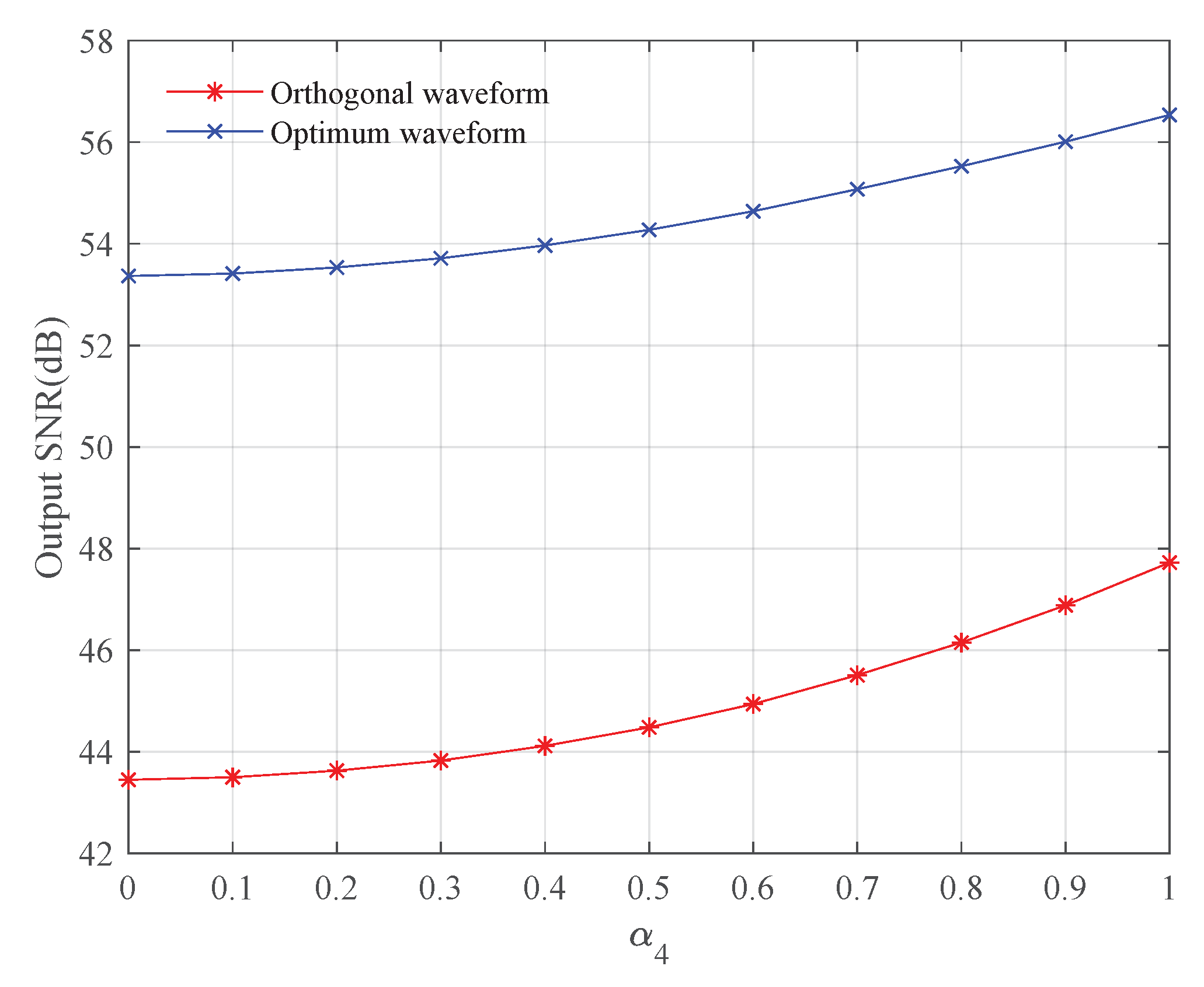
4.3. Output SNR with Different Amplitude Modulus Values

This experiment verifies the influence of multipath’s different amplitude modulus values on the output SNR. The number of multipath M is 4, and the DOAs of the former three paths are 2°, −2°, 4°. The corresponding amplitude factors and the delays are $1.0000+0.0000i,0.8853-0.0402i,0.7005-0.0499i$ and 0 ns, 2 ns, 6 ns, respectively. These parameters remain unchanged throughout the simulation. For the last path, the delay and the DOA are $15ns$ and 10°. Its amplitude factor is ${\alpha }_4{e}^{j({160}^{\circ }/{180}^{\circ }\pi )}$, where the modulus ${\alpha }_4$ increases uniformly from 0 to 1 with an interval of 0.1 while the phase angle remains unchanged. Under SNR = 0 dB, we calculated the final SNR by averaging the output SNR of 100 Monte Carlo trails.

As shown in Figure 4, the output SNR increases with the increase of the multipath modulus value for both waveforms. Besides, the change rate of the output SNR is growing at the same time. It suggests that we can improve the output SNR by taking advantage of multipath’s energy. During the amplitude modulus value range, the output SNR of the optimum waveform always outperforms the orthogonal waveform. The result shows the effectiveness of the proposed algorithm in multipath environments.

5. Conclusions

In this letter, we design an adaptive TR waveform covariance matrix for MIMO radar systems, which improves output SNR with multipath exploitation in diffuse multipath environments. Simulation results verify that multipath is suitable for enhancing the output SNR. Furthermore, the results illustrate the superiority of the designed waveform covariance matrix in different multipath environments by comparing it with the classical orthogonal waveform. In the future, we will research the waveform design of moving targets in multipath environments based on this algorithm.

References

1. Burkholder, R.J.; Pino, M.R.; Obelleiro, F. Low angle scattering from 2-D targets on a time-evolving sea surface. IEEE Trans. Geosci. Remote Sens. 2002, 40, 1185–1190. [Google Scholar] [CrossRef]
2. Feng, S.; Chen, J. Low-angle reflectivity modeling of land clutter. IEEE Geosci. Remote Sens. Lett. 2006, 3, 254–258. [Google Scholar] [CrossRef]
3. Niu, C.; Zhang, Y.; Guo, J. Low angle estimation in diffuse multipath environment by time-reversal minimum-norm-like technique. IET Radar Sonar Navig. 2017, 11, 1483–1487. [Google Scholar] [CrossRef]
4. Foroozan, F.; Asif, A.; Boyer, R. Time Reversal MIMO Radar: Improved CRB and Angular Resolution Limit. In Proceedings of the 2013 IEEE International Conference on Acoustics, Speech and Signal Processing, Vancouver, BC, Canada, 26–31 May 2013. [Google Scholar]
5. Hossain, M.D.; Mohan, A.S. Eigenspace Time-Reversal Robust Capon Beamforming for Target Localization in Continuous Random Media. IEEE Antennas Wirel. Propag. Lett. 2017, 16, 1605–1608. [Google Scholar] [CrossRef] [Green Version]
6. Sajjadieh, M.H.; Asif, A. Compressive sensing time reversal mimo radar: Joint direction and doppler frequency estimation. IEEE Signal Process. Lett. 2015, 22, 1283–1287. [Google Scholar] [CrossRef]
7. Foroozan, F.; Asif, A.; Jin, Y.; Moura, J.M. Direction finding algorithms for time reversal MIMO radars. In Proceedings of the 2011 IEEE Statistical Signal Processing Workshop (SSP), Nice, France, 28–30 June 2011. [Google Scholar]
8. Cui, G.; Li, H.; Rangaswamy, M. MIMO Radar Waveform Design With Constant Modulus and Similarity Constraints. IEEE Trans. Signal Process. 2014, 62, 343–353. [Google Scholar] [CrossRef]
9. Du, X.; Aubry, A.; Maio, A.D.; Cui, G. Hidden Convexity in Robust Waveform and Receive Filter Bank Optimization Under Range Unambiguous Clutter. IEEE Signal Process. Lett. 2020, 27, 885–889. [Google Scholar] [CrossRef]
10. Imani, S.; Ghorashi, S.A.; Bolhasani, M. SINR maximization in colocated MIMO radars using transmit covariance matrix. Signal Process. 2016, 119, 128–135. [Google Scholar] [CrossRef]
11. Haghnegahdar, M.; Imani, S.; Ghorashi, S.A.; Mehrshahi, E. SINR Enhancement in Colocated MIMO Radar Using Transmit Covariance Matrix Optimization. IEEE Signal Process. Lett. 2017, 24, 339–343. [Google Scholar] [CrossRef]
12. Chen, C.; Vaidyanathan, P.P. MIMO Radar Waveform Optimization With Prior Information of the Extended Target and Clutter. IEEE Trans. Signal Process. 2009, 57, 3533–3544. [Google Scholar] [CrossRef]
13. Sharma, A.; Ram, S.S. MIMO waveform design for minimizing multipath from ground and ceiling reflections. In Proceedings of the 2015 IEEE International Symposium on Antennas and Propagation and USNC/URSI National Radio Science Meeting, Vancouver, BC, Canada, 19–24 July 2015. [Google Scholar]
14. Chakraborty, B.; Li, Y.; Zhang, J.J.; Trueblood, T.; Papandreousuppappola, A.; Morrell, D. Multipath exploitationwith adaptivewaveform design for tracking in urban terrain. In Proceedings of the IEEE International Conference on Acoustics Speech and Signal Processing, Dallas, TX, USA, 14–19 March 2010. [Google Scholar]
15. Foroozan, F.; Asif, A. Time reversal MIMO radar for angle-Doppler estimation. In Proceedings of the 2012 IEEE Statistical Signal Processing Workshop (SSP), Ann Arbor, MI, USA, 5–8 August 2012; pp. 860–863. [Google Scholar]
16. Foroozan, F.; Asif, A.; Jin, Y. Cramer-Rao bounds for time reversal mimo radars with multipath. IEEE Trans. Aerosp. Electron. Syst. 2016, 52, 137–154. [Google Scholar] [CrossRef]
17. Jin, Y.; Moura, J.M.; O’Donoughue, N.; Harley, J. Single antenna time reversal detection of moving target. In Proceedings of the 2010 IEEE International Conference on Acoustics, Speech and Signal Processing, Dallas, TX, USA, 14–19 March 2010; pp. 3558–3561. [Google Scholar]
18. He, H.; Li, J.; Stoica, P. Waveform Design for Active Sensing Systems: Narrowband Beampattern to Covariance Matrix; Cambridge University Press: New York, NY, USA, 2012; pp. 187–212. [Google Scholar]
Figure 1. Multipath system model.
Remotesensing 12 03565 g001
Figure 2. The output SNR versus input SNR.
Remotesensing 12 03565 g002
Figure 3. The output SNR with different numbers of multipath.
Remotesensing 12 03565 g003
Figure 4. The output SNR with different amplitude modulus values.
Remotesensing 12 03565 g004