Abstract
Land cover maps are important tools for quantifying the human footprint on the environment and facilitate reporting and accounting to international agreements addressing the Sustainable Development Goals. Widely used European land cover maps such as CORINE (Coordination of Information on the Environment) are produced at medium spatial resolutions (100 m) and rely on diverse data with complex workflows requiring significant institutional capacity. We present a 10 m resolution land cover map (ELC10) of Europe based on a satellite-driven machine learning workflow that is annually updatable. A random forest classification model was trained on 70K ground-truth points from the LUCAS (Land Use/Cover Area Frame Survey) dataset. Within the Google Earth Engine cloud computing environment, the ELC10 map can be generated from approx. 700 TB of Sentinel imagery within approx. 4 days from a single research user account. The map achieved an overall accuracy of 90% across eight land cover classes and could account for statistical unit land cover proportions within 3.9% (R2 = 0.83) of the actual value. These accuracies are higher than that of CORINE (100 m) and other 10 m land cover maps including S2GLC and FROM-GLC10. Spectro-temporal metrics that capture the phenology of land cover classes were most important in producing high mapping accuracies. We found that the atmospheric correction of Sentinel-2 and the speckle filtering of Sentinel-1 imagery had a minimal effect on enhancing the classification accuracy (<1%). However, combining optical and radar imagery increased accuracy by 3% compared to Sentinel-2 alone and by 10% compared to Sentinel-1 alone. The addition of auxiliary data (terrain, climate and night-time lights) increased accuracy by an additional 2%. By using the centroid pixels from the LUCAS Copernicus module polygons we increased accuracy by <1%, revealing that random forests are robust against contaminated training data. Furthermore, the model requires very little training data to achieve moderate accuracies—the difference between 5K and 50K LUCAS points is only 3% (86% vs. 89%). This implies that significantly less resources are necessary for making in situ survey data (such as LUCAS) suitable for satellite-based land cover classification. At 10 m resolution, the ELC10 map can distinguish detailed landscape features like hedgerows and gardens, and therefore holds potential for aerial statistics at the city borough level and monitoring property-level environmental interventions (e.g., tree planting). Due to the reliance on purely satellite-based input data, the ELC10 map can be continuously updated independent of any country-specific geographic datasets.
1. Introduction
Satellite-based remote sensing of land use and land cover has afforded dynamic monitoring and quantitative analysis of the human footprint on the biosphere [1]. This is important because land cover change is a significant driver of the global carbon cycle, energy balance and biodiversity changes [2,3] which are processes of existential consequence. Land cover maps are often the primary inputs into accounting frameworks that attempt to monitor countries’ efforts towards addressing the Sustainable Development Goals (SDGs) [4]. For instance, land cover maps are often used to set targets and indicators for meeting SDG 2 of zero hunger and SDG 15 to monitor efforts to reduce natural habitat loss (e.g., deforestation alerts). Ecosystem service models and accounts also rely on land cover data as input [5] and land cover maps are thereby important for the valuation and conservation of important ecosystems. In light of global climate change and a rapidly developing world, an increasing number of applications, such as precision agriculture, wildlife habitat management, urban planning, and renewable energy installations, require higher resolution and frequently updated land cover maps.
The advent of cloud computing platforms like the Google Earth Engine [6] has led to significant advances in the ability to map land surface changes over time [7,8]. This is both due to the enhanced computing power and the availability of dense time series data from medium to high resolution sensors like Sentinel-2 [9]. The transition to time series imagery allows one to capture the seasonal and phenological components of land cover classes that would otherwise be missed with single time-slice imagery. The application of such spectro-temporal metrics to mapping forest [10] and other land cover types [11] has shown increased classification accuracies. In addition, the ability to adopt machine learning algorithms in cloud computing environments has further enhanced the precision of land cover mapping [4].
The CORINE (Coordination of Information on the Environment) land cover map of Europe [12] is perhaps the most widely used land cover product for area statistics and research [13]. The CORINE map currently requires significant institutional capacity and coordination from the European member states, the Eionet network, and the European Environmental Agency. For instance, the 2012 product involved 39 countries, a diversity of country-specific topographic and remote sensing datasets and took two years to complete. To ease the manual workload, the wealth of data from the Copernicus Sentinel sensors has been somewhat integrated into the CORINE mapping workflow and has also led to the development of Copernicus Land cover services high spatial resolution maps (https://land.copernicus.eu/pan-european/high-resolution-layers, accessed on 15 May 2021). Recently, Sentinel-2 data have been used to create a 10 m pan-European land cover/use map (S2GLC) for cairca 2017 (http://s2glc.cbk.waw.pl/, accessed on 15 May 2021) [14]. This is a meaningful advancement on previous pan-European mapping efforts, however, the methodology behind S2GLC involves a land cover reference dataset and some post-processing steps that are not open source or easily reproducible. Pflugmacher et al. [15] recently developed an independent, research-driven approach to pan-European land cover mapping with Landsat data at 30 m for cairca 2015. This compares favourably with the CORINE map, is reproducible and does not require harmonising and collating country-specific datasets from different European member states. Nevertheless, there remains potential for a similar open source approach that leverages both Sentinel-2 optical and Sentinel-1 radar sensor data to map land cover at 10 m resolution [16].
Land cover maps made with open data policies and open science principles can have transfer value to other areas of the globe [17], particularly when pre- and post-processing decisions are made transparent. Like the European maps mentioned above, the studies documenting continental land cover classifications at 30- or 10-m resolution for Africa [18,19], North America [20] and Australia [21] have not communicated methodological lessons or published source codes. The same is true for global land cover products such as the Landsat-based GLOBLAND30 [22] or Sentinel-based FROM-GLC10 [23]. This makes it difficult to draw generalizable conclusions that the benefit of remote sensing and the land cover mapping community at large. Specifically, it is not clear how satellite and reference data pre-processing decisions affect the accuracy of land cover classifications at this scale. Such decisions may concern the atmospheric correction of optical imagery (Sentinel-2), the speckle filtering of radar imagery (Sentinel-1), or the fusion of optical and radar data within one classification model. When trying to classify land cover over very broad environmental gradients where spectral signatures vary substantially within a given land cover class, one may also decide to include auxiliary variables to increase model accuracy [15]. Such decisions have trade-offs between computational efficiency and classification accuracy which are important to quantify when operationalising land cover classification at continental scales.
Another important point of consideration in operational land cover classification is the collection and cleaning of reference data (“ground-truth”) that are used to train a classification model. The quality, quantity and representativity of reference data can have significant effects on the accuracy and consequent utility of a land cover map [17]. In Europe, the Land Use/Cover Area Frame Survey (LUCAS) dataset consists of in situ land cover data collected over a grid of point locations over Europe [24]. However, when aligning satellite pixels data with LUCAS grid points, the geolocation uncertainty in both datasets can lead to mislabelled training data for land cover classification. To make LUCAS data suitable for earth observation, EUROSTAT introduced a new module (i.e., the Copernicus module) to the LUCAS survey in 2018 [25]. The Copernicus module has quality-assured and transformed 58,428 of the LUCAS points into polygons of homogeneous land cover that are suitable for earth observation purposes. Given that Weigand et al. [26] have shown that intersecting Sentinel pixels with LUCAS grid points already yields accurate land cover classifications, it remains to be seen how the inclusion of the Copernicus LUCAS polygons improves classification accuracy. Furthermore, previous attempts to integrate LUCAS data with remote sensing for land cover classification [15,26,27] have not fully assessed the trade-off between the reference sample size, model accuracy and the spatial distribution of prediction uncertainty. This information is important for planning future ground-truth data collection missions and remote sensing integrations.
Here, we aimed to build upon previous efforts to generate a 10 m Sentinel-based pan-European land cover map (ELC10) for 2018 using a reproducible and open source machine learning workflow. In doing so, we aim to explicitly test the effect of several pre-model data processing decisions that are often overlooked. Concerning satellite data processing, these include the effect of (1) Sentinel-2 atmospheric correction; (2) Sentinel-1 speckle filtering; (3) fusion of optical and radar data; and (4) addition of auxiliary predictor variables. Concerning land cover reference data, we aim to test the effect of (5) quality-checking reference points through the use of the LUCAS Copernicus module, and (6) the effect of decreasing the reference sample size. Finally, we compare ELC10 to existing land cover maps both in terms of accuracy and utility accounting for area statistics.
2. Methods
2.1. Study Area
We defined the scope of our study area to include all of Europe from 10°W to 30°E longitude and 35°N to 71°N latitude, except for Iceland, Turkey, Malta and Cyprus (Figure 1). This area is similar to the CORINE Land Cover product produced by the Copernicus Land Monitoring Service covering the European Economic Area of 39 countries and approximately 5.8 million square kilometres. Europe covers a wide range of climatic and ecological gradients primarily explained by the North–South latitudinal gradient [28]. Southern regions are arid warmer climates supporting a diverse range of Mediterranean vegetation. Northern regions are mesic, cooler climates characteristic of Boreal and Atlantic zones with shorter growing seasons and lower population densities leading to forest-dominated landscapes. Europe has a significant anthropogenic footprint with 40% of the land covered by agriculture, including semi-natural grasslands.
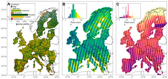
Figure 1.
Study area with available land cover reference points (A) and Sentinel (B,C) satellite imagery. Each point in (A) is a sampling location (53,476 polygons and 282,854 points) with a land cover class label. The number of available cloud-free Sentinel-2 pixels and Sentinel-1 pixels during 2018 are mapped in (B) and (C), respectively.
2.2. Land Cover Reference Data
LUCAS is a European Union initiative to gather in situ ground-truth data on land cover over 27 member states and is updated every three years [29]. It excludes Norway, Switzerland, Liechtenstein, and the non-EU Balkan states. Each iteration includes visiting a sub-sample of the 1,090,863 geo-referenced points within the LUCAS 2 km point grid. Under the 2018 LUCAS Copernicus module, 58,428 of the point locations have been quality assured and transformed into polygons of homogenous land cover specifically tailored for earth observation (Figure 2). The polygons are approximately 0.5 ha in size and are therefore (by design) large enough so that at least one Sentinel 10 × 10 m pixel is contained fully within them with some space for registration error. We used the collated and cleaned Copernicus Module polygon dataset (n = 53,476) provided by d’Andrimont et al. [25]. The centroid points of the Copernicus Module polygons (hereafter referred to as LUCAS polygon centroids) were used as the core of our reference sample for land cover classification. The top-level of the LUCAS land cover typology was used in the present analysis including artificial land, cropland, woodland, shrubland, grassland, bare land, wetland and water (Table 1).
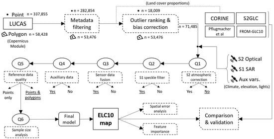
Figure 2.
Methodological workflow for evaluating the pre-processing of decisions in generating the final ELC10 land cover map. Underlined outcomes are those that were chosen for the final model. Abbreviations: S1—sentinel 1; S2—sentinel 2; Aux vars—auxiliary variables.

Table 1.
Land cover typology adopted along with LUCAS codes and descriptions.
After establishing baseline land cover proportions using the CORINE land cover dataset (re-coded to our typology) as a reference [12], we found that the distribution of the LUCAS polygons were biased toward cropland and woodland land cover classes (Figure S1). Consequently, there were very few LUCAS polygons for water, wetland, bare land and artificial land classes (Figure S1). We therefore performed a bias correction of the reference sample (Figure 2) by using the harmonised LUCAS theoretical grid point (hereafter LUCAS points) data [24] to supplement the LUCAS polygon centroid dataset so that the overall reference sample was representative of the CORINE proportions. Although the LUCAS theoretical points have not been transformed into polygons, they are still appropriate for earth observation applications [15] after applying certain quality control procedures. We employed the metadata filtering (Figure 2) outlined in Weigand et al. [26] to filter out points where the land cover parcel area was <0.5 ha, or covered <50% of the parcel. As in Pflugmacher et al. [15], we also excluded classes with potential thematic and spectral ambiguity including linear artificial features (LUCAS LC1 code A22), other artificial areas (A39), temporary grasslands (B55), spontaneously re-vegetated surfaces (E30) and other bare land (F40). This resulted in 282,854 labelled point locations available to supplement the LUCAS polygon sample. Of these, 18,009 LUCAS points were selected following an outlier ranking procedure to remove mislabelled or contaminated LUCAS points.
The outlier ranking procedure involved extracting Sentinel-2 data (see Section 2.3. for details) for pixels intersecting LUCAS points. These were fed into a random forest (RF) classification model (see Section 2.5 for details) which was used to calculate classification uncertainty for each LUCAS point. The RF model iteratively selects a random subset of data to generate decision trees which are validated against the withheld data. During each iteration, the model generates votes for the most likely class label. We extracted the fraction of votes for the correct land cover class at each LUCAS point after bootstrapping the RF procedure 100 times. We acknowledge that this bootstrapping of the RF model itself may not be necessary, however, it may smooth over any artifacts introduced from the internal bootstrapping of a single RF model. LUCAS points with a high fraction of votes (close to 1) can be considered as archetypal instances of the given land cover class, whereas those with a low fraction of votes (close to 0) are considered as mislabelled or spectrally contaminated. We ranked the LUCAS points by their fraction of correct votes and selected the topmost points for each land cover class to supplement the LUCAS polygon centroids so that the final land cover proportions matched that of the CORINE dataset. The number of supplemental LUCAS points needed (n = 18,009) was determined as relative to the most abundant LUCAS polygon class (cropland in Figure S1).
2.3. Sentinel Spectro-Temporal Features
All remote sensing analyses were conducted in the Google Earth Engine cloud computing platform for geospatial analysis [6]. We processed all Sentinel-2 optical and Sentinel-1 synthetic aperture radar (SAR) scenes over Europe during 2018. This amounts to a total of 239,818 satellite scenes which would typically require approx. 700 TB storage space if not for Google Earth Engine and cloud computation. The Sentinel satellite data were used to derive spectro-temporal features as predictor variables in our land cover classification model. Spectro-temporal features were used to capture both the spectral and temporal (e.g., phenology or crop cycle) characteristics of land cover classes and offer enhanced model prediction accuracy compared to single time-point image classification [15,30]. To generate model training data, spectro-temporal metrics were extracted for Sentinel pixels intersecting the LUCAS points, or the centroids of the LUCAS polygons.
Sentinel-2 images for both Top of Atmosphere (TOA; Level 1C) and Surface Reflectance (SR; Level-2A) were used to test the effect of atmospheric correction on classification accuracies (Q1 in Figure 2). The scenes were first filtered for those with less than 60% cloud cover (129,839 removed of 280,420 scenes) using the “CLOUDY_PIXEL_PERCENTAGE” scene metadata field. We then performed a pixel-wise cloud masking procedure using the cloud probability score produced by the S2cloudless algorithm [31]. S2cloudless is a machine learning-based algorithm and is part of the latest generation of cloud detection algorithms for optical remote sensing images. After visually inspecting the cloud masking results across a range of Sentinel-2 scenes, we settled on a cloud probability threshold of 40% for our masking procedure. After cloud masking and mosaicking two years’ worth of Sentinel-2 scenes, the cloud-free pixel availability ranged from less than 10 to over 100 pixels over the study area (Figure 1B).
Using the cloud-masked Sentinel-2 imagery, we derived the median mosaic of all spectral bands. The median mosaic was derived by calculating the pixel-wise median value across the time series of images within the year. In addition, we calculated the following spectral indices for each cloud-masked scene: normalised difference vegetation index [32], normalised burn ratio [33], normalised difference built index [34], and normalised difference snow index [35]. For each spectral index, we used the temporal resolution to calculate the 5th, 25th, 50th, 75th and 95th percentile mosaics as well as the standard deviation, kurtosis and skewness across the two-year time stack of imagery. We derived the median NDVI values for the summer (June–August), winter (December–February), spring (March–May), and fall (September–November). The spectro-temporal metrics described above have been extensively used to map land cover and land use changes with optical remote sensing [36]. Finally, several studies have found that textural image features (i.e., defining pixel values from those of their neighbourhood) for Sentinel-2 imagery significantly enhanced land cover classification accuracy [26,37]. Therefore, we calculated the standard deviation of median NDVI within a 5 × 5 pixel moving window.
Sentinel-1 SAR Ground Range Detected data were pre-processed by Google Earth Engine, including thermal noise removal, radiometric calibration and terrain correction using global digital elevation models. Sentinel-1 scenes were filtered for interferometric wide swath and a resolution of 10 m to suit our land cover classification purposes. We performed an angular-based radiometric slope correction using the methods outlined in Vollrath et al. [38]. SAR data can contain a substantial speckle and backscatter noise which is important to address particularly when performing pixel-based image classification. We applied a Lee-sigma speckle filter [39] to the Sentinel-1 imagery to test the effect on classification accuracy (Q2 Figure 2). Following pre-processing, we calculated the median and standard deviation mosaics for the time stacks of imagery including the single co-polarised, vertical transmit/vertical receive (VV) band and the cross-polarised, vertical transmit/horizontal receive (VH) band, as well as the ratio between them (VV/VH).
2.4. Auxiliary Features
A challenge of classifying regional-scale land cover is that models relying on spectral responses alone may be limited by the fact that land cover characteristics can change drastically between climate and vegetation zones. For example, a grassland in the Mediterranean will have very different spectro-temporal signatures to a grassland in the boreal zone. Previous regional land cover classification efforts have dealt with this by either (1) splitting the area up into many small parts and running multiple classification models [20], or (2) including environmental covariates that help the model explain the regional variation in land cover characteristics [15,40]. We tested the latter approach (Q4 in Figure 2) by including a range of environmental auxiliary covariates into our classification model.
Auxiliary variables included elevation data from the Shuttle Radar Topography Mission (SRTM) digital elevation dataset [41] at 30 m resolution which covers up to 60° north. For higher latitudes, we used the 30 arc-second elevation data from the United States Geological Survey (GTOPO30). Climate data were derived from the ERA5 fifth generation ECMWF atmospheric reanalysis of the global climate [42]. We used it to calculate the 10-year (2010–present) average and standard deviation in monthly precipitation and temperature at 25 km resolution. Finally, we also included data on night-time light sources at approx. 500 m spatial resolution. This was intended to assist the model in differentiating artificial surfaces and bare ground in alpine areas. A median 2018 radiance composite image from the Visible Infrared Imaging Radiometer Suite (VIIRS) Day/Night Band (DNB), provided by the Earth Observation Group, Payne Institute, was used [43].
2.5. Classification Models and Accuracy Assessment
The land cover classification model evaluation and tuning were conducted in R with the ‘randomForest’ and ‘caret’ packages (R Core Team, 2019), while the final model inference over Europe was conducted in Google Earth Engine using equivalent model parameters. We chose an ensemble learning method, namely the random forest (RF) classification model. RF deals well with large and noisy input data, accounts for non-linear relationships between explanatory and response variables, and is robust against overfitting [44]. A recent review of land cover classification literature found that the RF algorithm has the highest accuracy level in comparison with the other classifiers adopted [45]. Classification accuracies were determined using internal randomised cross-validation procedures where error rates are determined from the mean prediction error on each training sample xi, only using the trees that did not have xi in their bootstrap sample (i.e., out-of-bag; [46]). Predicted and observed land cover classes are used to build a confusion matrix from which one derives overall accuracy (OA), user’s accuracy (UA), and producer’s accuracy (PA). See Stehman and Foody [47] for details.
A series of RF models were run at each step in the pre-processing tests (Figure 2) in order to assess the effect of pre-processing decisions on classification accuracy. With each consecutive step, we chose the pre-processing option that yielded the highest accuracy to generate the data for the subsequent step. The final pre-processing sequence that led to the final RF model data were indicated by the underlined decisions in Figure 2. When testing the effect of reference sample size (Q6 in Figure 2), we iteratively removed 5% of the training dataset and assessed model performance. All 71,485 LUCAS locations (polygon centroids and theoretical points) were used to train the final RF model. At this stage we performed recursive feature elimination which is a process akin to backward stepwise regression that prevents overfitting and reduces unnecessary computational load [48]. Recursive feature elimination produces a model with the maximum number of features and iteratively removes the weaker variables until a specified number of features is reached. In our case, this was 15 features. The top predictor variables were selected based on the variable importance ranking using both the mean decrease in accuracy and mean decrease in Gini coefficient scores [49]. Finally, we also tuned the RF hyperparameters by iterating over a series of ntree (50 to 500 in 25 tree intervals) and mtry (1 to 10) and found the optimal (based on lowest model error rate) combination of settings to include a ntree of 100 and mtry set to the square root of the number of covariates (3.8).
Part of enhancing the usability of land cover maps is quantifying the spatial distribution of classification uncertainty. There are methods to derive pixel-based and sample-based uncertainty estimates that are spatially explicit [37,50,51]. We adopted a sample-based uncertainty estimate by dividing the study area into 100 km equal-area grid squares defined by the European Environmental Agency reference grid. For each grid cell, we use our final trained RF model to make predictions against the LUCAS reference data within and build a confusion matrix to derive overall accuracy for the grid cell in question. We acknowledge that making predictions over reference samples that were included in model training is likely to inflate accuracy estimates. However, in this case, we are interested in obtaining the relative distribution of accuracy over the study region to give insight into class non-separability and map reliability over space.
2.6. Comparison with Other Land Cover Maps
We compared our land cover product with two other global land cover products including CORINE [12], and FROM-GLC10 [23], and two other European land cover maps including the map created by Pflugmacher et al. [15] and S2GLC [14]. The CORINE map was updated for 2018 at 100 m resolution by the Copernicus Land Management Service and is widely used for aerial statistics and accounting. FROM-GLC10 is a global map produced with Sentinel satellite data at 10 m resolution. The S2GLC (Sentinel-2 Global Land Cover) map has been produced over Europe during 2017 using Sentinel 2 data at 10 m resolution. The Pflugmacher et al. [15] map was produced for 2015 using Landsat data at 30 m resolution. All land cover typologies were converted to the LUCAS typology used in our analysis for purposes of comparison (Table S1). The same accuracy assessment protocols described above were used to assess the accuracy of these maps using the same validation dataset (completely withheld from the training of our model).
Apart from assessing the classification accuracy, we tested the utility of the maps for calculating aerial land cover statistics over spatial units defined for the European Union by the nomenclature of territorial units (NUTS). We used NUTS level 2 basic regions which include population sizes between 0.8 and 3 million and are used for the application of regional policies. Area proportions for each land cover class and map product, including ELC10, were calculated for each of the NUTS polygons. Within each NUTS polygon, we also calculated the area proportions using the original LUCAS survey dataset. We regressed the mapped area proportions on the area proportions estimated from the LUCAS sample to assess the land cover map’s utility for land cover accounting. Although the statistics derived from LUCAS dataset also have uncertainty associated with them, they are considered the only harmonised dataset for area statistics in Europe and were therefore used as the benchmark with which we compared the land cover maps.
3. Results
3.1. Effects of Satellite Data Pre-Processing
The pre-processing of Sentinel optical and radar imagery had very little effect on the overall classification accuracy (Figure 3A,B). Specifically, the atmospheric correction of Sentinel-2 and speckle filtering of Sentinel-1 imagery enhanced the classification accuracy by less than 1% compared to models with TOA and non-speckle filtered imagery, respectively. This marginal difference was true for all class-specific accuracies (Figure S2). However, the fusion of Sentinel-1 and Sentinel-2 data within a single model increased accuracy by 3% compared to Sentinel-2 alone and by 10% compared to Sentinel-1 alone (Figure 3C). Class-specific accuracies reveal that models with Sentinel-1 data alone perform particularly badly when predicting wetland, shrubland and bare land classes (Figure S2c). In these instances, fusing both optical and radar data increases accuracy by up to 30% compared to Sentinel-1 data alone. The addition of auxiliary data (terrain, climate and night-time lights) increased accuracy by an additional 2% compared to a model with Sentinel data alone (Figure 3D). Auxiliary data have the largest benefits for bare land and shrubland classes (Figure S2d).
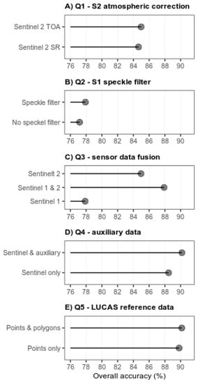
Figure 3.
The effect of pre-processing decisions on land cover classification accuracy. The random forest model overall accuracies are displayed for alternative Sentinel 2 (A), and 1 (B) pre-processing steps, Sentinel 1 and 2 data fusion options (C), the addition of auxiliary variables (D), and the quality of reference data (E). Each panel corresponds to a pre-processing decision in the workflow outlined in Figure 2. The option with the highest accuracy is utilised in the proceeding step.
3.2. Effects of Reference Data Pre-Processing
The first test of reference data pre-processing was a test of quality checking and cleaning the LUCAS data via the conversion of LUCAS points into homogenous polygons under the Copernicus module (Figure 2). Extracting the satellite data at LUCAS points vs. the centroids of homogenous LUCAS polygons increased accuracy by less than 1% (Figure 3E). This marginal effect was evident for all class-specific accuracy scores (Figure S2e). The second test related to reference data involved the iterative depletion of the sample size. The relationship between sample size and overall accuracy appears to follow an exponential plateau curve (Figure 4). The benefit to model accuracy gained by increasing sample size depletes so rapidly that, for example, when one increases from 5K to 20K points, accuracy increases by 0.15% per 1K points added, while when one increases from 55K to 70K points, accuracy increases by 0.015% per 1K points. Therefore, the difference between 5K and 50K LUCAS points is only 3% (86% vs. 89%; Figure 4). The same pattern is evident for class-specific accuracies. However, it is important to note that the variance in accuracy from the bootstrapped RF classifications increased as the number of training samples decreased.
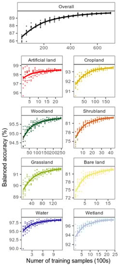
Figure 4.
The effect of the reference sample size on overall and class-specific accuracy. The random forest classification models were trained on iteratively smaller sample sizes. Points in each facet plot represent bootstrapped (n = 10) model accuracy estimates and are fit with Loess regression lines.
3.3. ELC10 Final Accuracy Assessment
The final RF classification model produced an overall accuracy of 90.2% across eight land cover classes (Table 2). The class-specific user’s accuracy (UA; errors of commission) describes the reliability of the map and informs the user of how well the map represents what is really on the ground. UA exhibited a wide range from 75% for shrubland to 96.4% for woodland. The relative decrease in prediction accuracy over shrubland classes is evident in the spatial distribution of model errors (Figure 5). The majority of the error (accuracies below 80%) was distributed over southern Europe where shrubland dominates (Figure 1A). Conversely, model accuracies were highest (above 90%) over the interior of Europe (Figure 5) where cropland and woodland dominate (Figure 1A). Shrubland was most often confused with grassland and woodland probably due to the spectral similarity across a gradient of woody plant cover. Similarly, cropland was most often confused with grassland probably due to the temporal similarity in spectral signatures between mowed pastures and ploughed fields.
Table 2.
Estimated error matrix for the final classification with estimates for user’s accuracy (UA) and producer’s accuracy (PA). Overall accuracy is 90.2%.
Figure 5.
Map showing land cover classification accuracy over 100 × 100 km grid squares. The inset bar plot shows the abundance of grid squares across the range of error (percentage overall accuracy). Missing grid cells are where there were insufficient validation samples to construct an error matrix.
Sentinel optical variables were the two most important covariates in the final RF model (Figure 6). The first and fifth most important variables were the 25th percentile of NDVI and standard deviation in NBR over time, respectively. These metrics both capture the temporal dynamics of spectral responses that are important in distinguishing land cover classes such as cropland and grassland. The Sentinel 1 VH band also exhibited a relatively high importance score. Of the auxiliary variables, night-time light intensity and temperature were the most important variables.
Figure 6.
Variable importance plot showing the relative contribution of the top 15 most influential predictor variables.
3.4. ELC10 Compared to Existing Maps
ELC10 produced by the final RF model compared favourably relative to two global and two European land cover products (Figure 7). The overall accuracy for the ELC10 map was 18% higher than the lower resolution CORINE map, and 17% higher than the global 10 m FROM-GLC10 map. In comparison to the European-specific products, our map produced a 5% greater overall accuracy. Specifically, ELC10 was 7% more accurate than S2GLC and 3% more accurate than Pflugmacher et al. ELC10 displayed class-specific accuracies that were slightly (<1%) lower than Pflugmacher et al. for wetland, bare land and cropland classes (Figure 7). Otherwise, the ELC10 class-specific accuracies were greater than those for the other maps in all other land cover classes. Notable improvements upon other maps include those for water and artificial land (Figure 7).
Figure 7.
Class-wise user’s and overall accuracy for different European land cover products. Horizontal lines and points show the accuracy achieved for each land cover map.
In terms of the maps’ utility for area statistics, the ELC10 map produced a strong correlation to official LUCAS-based statistics (high R2 and low mean absolute error; Figure 8E). Land cover class area estimates are within 4.19% of the observed value for ELC10. This error is marginally higher than the error from Pflugmacher et al. (0.16% higher), but lower than the error for the other maps. Perhaps the most significant advantage of the ELC10 map is only realised at the landscape scale. Figure 9 (and Figures S3–S5) illustrates the ability of the ELC10 map to distinguish detailed landscape elements like hedge rows and intra-urban green spaces which are lost in the other lower-resolution products.
Figure 8.
Correlation of mapped land cover proportions with LUCAS accounting for the statistics of each European land cover product. Each datum point represents the proportion for a NUTS level 2 statistical unit. Coloured linear regression lines are fitted per land cover class with an overall regression in black. Overall regression R2, root mean square error (RMSE) and mean absolute error (MAE) are reported.
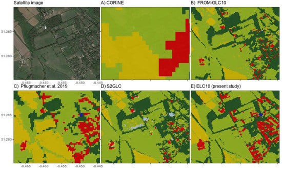
Figure 9.
Example of land cover classifications at the local scale for a selected landscape in Woking (south of London, England). Maps are shown for the present study relative to the four comparative datasets. Please refer to Supplementary Figures S3–S5 for more comparative examples.
4. Discussion
4.1. Comparison to State of the Art
The ELC10 map produced here has accuracy levels (90.2%) that are comparable with multiple city- and country-scale Sentinel-based land cover maps globally [16]. Within the European context, we find that ECL10 has 18% less error than the CORINE dataset which is widely used for research and accounting purposes. This corroborates results from others [15,52] who have also found uncertainty and bias associated with CORINE maps. The primary explanation for this discrepancy in accuracy is that the CORINE minimum mapping unit (25 ha) is very coarse compared to Landsat- and Sentinel-based maps (e.g., ELC10 minimum mapping unit of 0.01 ha). The CORINE project also adopts a bottom-up approach of consolidating nationally produced land cover datasets into one and is therefore prone to inconsistencies and spatial variations in mapping error. Although CORINE has been effectively used to stratify the probabilistic sampling of land cover for unbiased area estimates [53], it may not be functional in small municipalities or for other land use and ecosystem models that require fine-grained spatial data.
To address the need for fine-grained land cover data, the European Space Agency recently initiated the development of the S2GLC map over Europe at 10 m resolution (http://s2glc.cbk.waw.pl/) [14]. The ELC10 map produced here extends on the S2GLC work by improving the overall accuracy by 7% and adopting an open source and transparent approach in a similar vein to the Landsat-based map by Pflugmacher et al. [15]. Unlike previous pan-European maps, our approach relies on purely satellite-based input data and is therefore annually updatable for the foreseeable future lifespan of Sentinel and VIIRS sensors (assuming accuracy levels from LUCAS 2018 survey). It is thus independent of national topographic mapping datasets that take considerable resources to update (e.g., national land resource map of Norway; [54]. ELC10 also leverages Google’s cloud computing infrastructure, made freely available for research purposes through Google Earth Engine. We were able to train and make inference with our random forest model over 700 TB of satellite data at a rate of 100,000 km2 per hour which equates to approx. 4 days of computing time to generate the 10 m product for Europe. In this way, regional or continental scale mapping of land cover, which has typically been the domain of large transnational institutions, may become more democratised and independent of political agenda [55].
4.2. Potential Applications
As satellite technology and cloud computing improve, the ability to map land cover at high spatial resolutions is becoming increasingly possible. This opens up a range of novel use-cases for land cover maps at continental scales. One example is for mapping small patches of green space within and outside of urban areas. Rioux et al. [56] found that urban green space cover and associated ecosystem services were generally underestimated at spatial resolutions coarser than 10 m. Similarly, green spaces constituting important habitat for biodiversity such as semi-natural grasslands are often not portrayed in current land cover maps. This is significant given that habitat loss is one of the main threats facing biodiversity, particularly pollinator species, in agricultural landscapes across Europe [57,58]. Quantifying and monitoring the remaining fragmented habitat is therefore a conservation concern at both regional and national levels [59]. This is also true for monitoring the corollary of habitat loss–habitat restoration initiatives. Agri-environmental schemes [60] such as the establishment of stone walls, hedge rows, and strips of semi-natural vegetation along field margins are not detected by current land cover mapping initiatives. High-resolution land cover maps such as the ELC10, presented here, provide a means to monitor the status and trends of the remaining patches of semi-natural habitats and other small green spaces over Europe. It is also possible to extend this mapping workflow to areas outside of the European continent assuming there are reference data to calibrate the RF model. This Google Earth Engine workflow may be particularly beneficial in monitoring tropical ecosystems such as mangrove forests [61].
4.3. Limitations and Opportunities
As with all land cover products, there are several limitations to ELC10 that are important to note in the interest of data users and future iterations of pan-European land cover maps. Our model produced classification errors that were greatest (accuracies below 80%) in southern Europe due to the predominance of, and spectral similarity between shrubland and bare land classes. For future refinements of the map one could aim to partition the LUCAS shrubland class into, e.g., 2–3 levels of vegetational succession. Although some regions (i.e., central Europe, Figure 5) and classes (i.e., woodland: 95%, Table 2) exhibited much higher accuracies than southern Europe, the error rate may still be significant, particularly in the context of monitoring land use changes. A 95% accuracy implies that a land cover class would have to change by 10% within a spatial unit (e.g., country or municipality) from year to year in order for a map like ELC10 to detect it with statistical confidence.
A major source of error in land cover models is the reference data. The LUCAS dataset is vulnerable to geolocation errors due to GPS malfunctioning in the field, interpretation errors and land cover ambiguities. For instance, the European Environment Agency found that a post-screening of the LUCAS dataset increased CORINE-2000 accuracy by 6.4 percentage points [62]. In addition to mislabelled LUCAS points, intersecting Sentinel pixels may contain mixed land cover classes and therefore introduce noise into the spectral signal [25]. This is why the LUCAS Copernicus Module was initiated to produce quality-assured homogeneous polygons for integration with earth observation. However, here we found that intersecting Sentinel pixels with LUCAS polygon centroids did not significantly improve classification accuracy relative to the raw theoretical LUCAS point locations alone (Figure 3E). This finding supports the well-established characteristic of random forest models which makes them robust against noisy training data [63]. It remains to be seen whether utilising all pixels within LUCAS polygons increases accuracy further.
Users of ELC10 should also be aware that our classification model is extrapolating into areas without any reference data in countries including Norway, Switzerland, Liechtenstein, and the non-EU Balkan states. However, because the LUCAS data cover a broad range of environmental conditions, it is reasonable to assume similar accuracies for neighbouring countries, although this needs to be tested. The efficacy of integrating ground reference samples with remote sensing may be illustrative for Norway and other countries and stimulate future open-access land cover surveys. The fact that we found accuracies >85% with <5K reference points (Figure 4) should act as encouragement because it shows that land cover mapping with earth observation does not necessarily require large resources dedicated to reference data collection. However, the variance in classification accuracy increases substantially with a reduction in reference sample size, and therefore, this might limit the ability to make accurate models at both the national and continental scale. Alternatives to in situ sampling include less resource-intensive methods, commonly adopted in the deforestation monitoring community, such as visual interpretation of very high resolution satellite or aerial imagery in platforms like Collect Earth Online [64].
There remain several avenues for improving upon ELC10 and Sentinel-based land cover mapping which may strengthen its utility for research and policy purposes. The harmonisation of Landsat and Sentinel time series [65] may enhance the benefit gained from spectro-temporal features. This may be particularly beneficial in areas with high cloud cover, which creates gaps in the Sentinel-2 time series and consequent noise in the spectro-temporal features. The use of repeat-pass SAR interferometry may also enhance accuracy [66] beyond that achieved here because we were limited to using Sentinel-1 Ground Range Detected data, that are analysis-ready in Google Earth Engine. In this particular case, Google Earth Engine is limited and one might explore other cloud computing platforms such as Sentinel Hub, Open Data Cube, Copernicus DIAS, the European Open Science Cloud, or custom set-ups in Microsoft Azure or Amazon Web Services [67]. Other cloud computing platforms may also offer a suite of other machine learning algorithms under the deep learning umbrella, such as neural networks, which may produce greater accuracies than classification tree approaches like RF [68]. Recently, Google Earth Engine has developed an integration with the machine learning platform TensorFlow which allows for the application of deep learning algorithms to land cover classification (e.g., [69,70]).
Finally, research on mapping uncertainty is an ongoing need. This is particularly true for quantifying uncertainty associated with land cover change statistics [71] derived from Sentinel land cover maps. Land cover change from Sentinel data may be assessed with the next iteration of LUCAS in 2022, or with the harmonised historical data provided by d’Andrimont et al. [24]. Quantifying uncertainty is necessary for such maps to be included into governmental and municipal accounting frameworks that ultimately contribute to addressing the global SDGs. Khatami et al. [37] reviewed a range of methods to derive pixel-level estimates of uncertainty, many of which rely on producing a posteriori class probabilities obtained from the random forest classifier. Class probabilities may also be used to perform post-processing steps that remove artifacts and the salt-and-pepper effects of pixel-based classification, such as in Malinowski et al. [14].
4.4. Recommendations
We attempted to maintain transparency in the data pre-processing decisions we made by presenting the effects on model accuracy at each step (Figure 2). Although our findings are not necessarily generalizable to areas outside of Europe, they are useful guidelines for others to learn from. Based on our experience, we recommend the following for future Sentinel-based land cover mapping at the continental scale:
- The atmospheric correction of Sentinel-2 optical has marginal effects on classification accuracy and therefore may be skipped. This is supported by other studies (Rumora et al., 2020) and is particularly relevant when users are interested in near-real time land cover classification because Top of Atmosphere products are generally made available before surface reflectance products.
- Applying a speckle filter to Sentinel-1 imagery has marginal effects on classification accuracy and therefore may be skipped. As far as we are aware, there are no other studies that have tested this effect. Applying speckle filtering is computationally intensive and therefore excludes its benefit of fast and on-the-fly land cover classifications where desirable. However, we acknowledge that we only used a single median and standard deviation per band and orbit mode for a full year of data. Speckle filtering may be more effective if one derives seasonal or monthly composites as inputs into the classifier, as we did with Sentinel-2 NDVI.
- The fusion of Sentinel-1 and Sentinel-2 data has large increases in classification accuracy (3–10%) and is therefore encouraged. The addition of auxiliary variables that capture large-scale environmental gradients important for distinguishing spectrally similar classes (e.g., shrubland and forest) also improve classification accuracies and should be included. However, users should be cautious of spatial overfitting to these auxiliary variables which may cause geographical biases due to spatial autocorrelations [72,73].
- Cleaning reference samples through initiatives like the LUCAS Copernicus Module may not be worth the marginal gains in classification accuracy. RF models are robust against noisy training data [63] and therefore, so long as a clean validation sample is maintained, filtering noise in training data may not be necessary. Nevertheless, clean reference data supplied by the Copernicus Module is invaluable to deriving realistic accuracy estimates. We supplemented the Copernicus Module polygons with LUCAS points (n = 18,009) in order to balance class representativity in the training sample. We did this using an outlier removal procedure which may have artificially inflated our final accuracy estimates. Therefore, we recommend that initiatives like the Copernicus Module ensure that their sample is representative of the class area proportions in the study area, so that augmenting the training sample is not necessary for earth observation applications in the future.
- Collecting tens of thousands of reference data points may also not be necessary depending on the desired classification accuracy. We found that accuracies above 85% are achievable with less than 5000 LUCAS points, albeit for an eight-class classification typology.
- Cloud computing infrastructure like Google Earth Engine make ideal platforms given that we could produce a pan-European map within approx. 4 days of computation time from a single research user account.
5. Conclusions
The recent proliferation of freely available satellite data in combination with advances in machine learning and cloud computing has heralded a new age for land cover classification. What has previously been the domain of transnational institutions, such as the European Space Agency, is now open to individual researchers and members of the public. We present ELC10 as an open source and reproducible land cover classification workflow that adheres to open science principles and democratises large scale land cover monitoring. We find that combining Sentinel-2 and Sentinel-1 data is more important for classification accuracy than the atmospheric correction and speckle filtering pre-processing steps individually. We also confirm the findings of others that the random forest is robust against noisy training data, and that investing resources in collecting tens of thousands of ground-truth points may not be worth the gains in accuracy. Despite the effects of data pre-processing, ELC10 has unique potential for quantifying and monitoring detailed landscape elements important to climate mitigation and biodiversity conservation such as urban green infrastructure and semi-natural grasslands. Looking to the future, maps like ELC10 can be annually updated, and repeated in situ surveys like LUCAS can be used for quantifying uncertainty and accuracy in area change estimates. Quantifying uncertainty is crucial for earth observation products to be taken seriously by policy makers and land use planners.
Supplementary Materials
The following are available online at https://www.mdpi.com/article/10.3390/rs13122301/s1, Figure S1: Distribution of LUCAS reference points used in the final ELC10 model (n = 71,485) across land cover classes. LUCAS polygons were supplemented with LUCAS points so that the samples sizes were proportional to the CORINE land cover proportions over Europe., Figure S2: The effect of pre-processing decisions on land cover classification accuracy per land cover class. Random Forest model class-specific balanced accuracies are displayed for alternative Sentinel 2 (A), and 1 (B) pre-processing steps, Sentinel 1 and 2 data fusion options (C), the addition of auxiliary variables (D), and the quality of reference data (E), Figure S3: Example of land cover classifications at the local scale for a selected landscape in Ozford, England. Maps are shown for the present study relative to the four comparative datasets, Figure S4: Example of land cover classifications at the local scale for a selected landscape east of Barcelona, Spain. Maps are shown for the present study relative to the four comparative datasets, Figure S5: Example of land cover classifications at the local scale for a selected landscape south of Tarcento, Italy. Maps are shown for the present study relative to the four comparative datasets, Table S1: Land cover maps used for comparison with ELC10 were relassified into the ELC10 (based on LUCAS high level typology) typology. The lookup tables to show reclassifications are presented below.
Author Contributions
Z.S.V. conceived the methodology, conducted the analysis and wrote the first draft. M.A.K.S. provided resources, assisted with conceptual development and contributed to the writing and draft revision. Both authors have read and agreed to the published version of the manuscript.
Funding
This research was funded, in whole or in part, by The Research Council of Norway [project number 302692]. For the purpose of open access, the author has applied a CC BY public copyright license to any Author Accepted Manuscript (AAM) version arising from this submission.
Institutional Review Board Statement
Not applicable.
Informed Consent Statement
Not applicable.
Data Availability Statement
The ELC10 dataset is available here: https://doi.org/10.5281/zenodo.4407051 JavaScript and R code to reproduce ELC10 is available here: https://github.com/NINAnor/ELC10.
Acknowledgments
We thank the anonymous reviewers for their constructive feedback.
Conflicts of Interest
The authors declare no conflict of interest.
References
- Chang, Y.; Hou, K.; Li, X.; Zhang, Y.; Chen, P. Review of Land Use and Land Cover Change Research Progress. IOP Conf. Ser. Earth Environ. Sci. 2018, 113, 012087. [Google Scholar] [CrossRef]
- Foley, J.A.; DeFries, R.; Asner, G.P.; Barford, C.; Bonan, G.; Carpenter, S.R.; Chapin, F.S.; Coe, M.T.; Daily, G.C.; Gibbs, H.K.; et al. Global Consequences of Land Use. Science 2005, 309, 570–574. [Google Scholar] [CrossRef]
- Maxwell, S.L.; Fuller, R.A.; Brooks, T.M.; Watson, J.E.M. Biodiversity: The Ravages of Guns, Nets and Bulldozers. Nat. News 2016, 536, 143. [Google Scholar] [CrossRef] [PubMed]
- Holloway, J.; Mengersen, K. Statistical Machine Learning Methods and Remote Sensing for Sustainable Development Goals: A Review. Remote Sens. 2018, 10, 1365. [Google Scholar] [CrossRef]
- De Araujo Barbosa, C.C.; Atkinson, P.M.; Dearing, J.A. Remote Sensing of Ecosystem Services: A Systematic Review. Ecol. Indic. 2015, 52, 430–443. [Google Scholar] [CrossRef]
- Gorelick, N.; Hancher, M.; Dixon, M.; Ilyushchenko, S.; Thau, D.; Moore, R. Google Earth Engine: Planetary-Scale Geospatial Analysis for Everyone. Remote Sens. Environ. 2017, 202, 18–27. [Google Scholar] [CrossRef]
- Mahdianpari, M.; Salehi, B.; Mohammadimanesh, F.; Brisco, B.; Homayouni, S.; Gill, E.; DeLancey, E.R.; Bourgeau-Chavez, L. Big Data for a Big Country: The First Generation of Canadian Wetland Inventory Map at a Spatial Resolution of 10-m Using Sentinel-1 and Sentinel-2 Data on the Google Earth Engine Cloud Computing Platform. Can. J. Remote Sens. 2020, 46, 15–33. [Google Scholar] [CrossRef]
- Tamiminia, H.; Salehi, B.; Mahdianpari, M.; Quackenbush, L.; Adeli, S.; Brisco, B. Google Earth Engine for Geo-Big Data Applications: A Meta-Analysis and Systematic Review. ISPRS J. Photogramm. Remote Sens. 2020, 164, 152–170. [Google Scholar] [CrossRef]
- Drusch, M.; Del Bello, U.; Carlier, S.; Colin, O.; Fernandez, V.; Gascon, F.; Hoersch, B.; Isola, C.; Laberinti, P.; Martimort, P.; et al. Sentinel-2: ESA’s Optical High-Resolution Mission for GMES Operational Services. Remote Sens. Environ. 2012, 120, 25–36. [Google Scholar] [CrossRef]
- Potapov, P.V.; Turubanova, S.A.; Tyukavina, A.; Krylov, A.M.; McCarty, J.L.; Radeloff, V.C.; Hansen, M.C. Eastern Europe’s Forest Cover Dynamics from 1985 to 2012 Quantified from the Full Landsat Archive. Remote Sens. Environ. 2015, 159, 28–43. [Google Scholar] [CrossRef]
- Azzari, G.; Lobell, D.B. Landsat-Based Classification in the Cloud: An Opportunity for a Paradigm Shift in Land Cover Monitoring. Remote Sens. Environ. 2017, 202, 64–74. [Google Scholar] [CrossRef]
- Büttner, G. CORINE land cover and land cover change products. In Land Use and Land Cover Mapping in Europe; Springer: Berlin/Heidelberg, Germany, 2014; pp. 55–74. [Google Scholar]
- Bielecka, E.; Jenerowicz, A. Intellectual Structure of CORINE Land Cover Research Applications in Web of Science: A Europe-Wide Review. Remote Sens. 2019, 11, 2017. [Google Scholar] [CrossRef]
- Malinowski, R.; Lewiński, S.; Rybicki, M.; Gromny, E.; Jenerowicz, M.; Krupiński, M.; Nowakowski, A.; Wojtkowski, C.; Krupiński, M.; Krätzschmar, E.; et al. Automated Production of a Land Cover/Use Map of Europe Based on Sentinel-2 Imagery. Remote Sens. 2020, 12, 3523. [Google Scholar] [CrossRef]
- Pflugmacher, D.; Rabe, A.; Peters, M.; Hostert, P. Mapping Pan-European Land Cover Using Landsat Spectral-Temporal Metrics and the European LUCAS Survey. Remote Sens. Environ. 2019, 221, 583–595. [Google Scholar] [CrossRef]
- Phiri, D.; Simwanda, M.; Salekin, S.; Nyirenda, V.R.; Murayama, Y.; Ranagalage, M. Sentinel-2 Data for Land Cover/Use Mapping: A Review. Remote Sens. 2020, 12, 2291. [Google Scholar] [CrossRef]
- Chaves, M.E.D.; Picoli, M.C.A.; Sanches, I.D. Recent Applications of Landsat 8/OLI and Sentinel-2/MSI for Land Use and Land Cover Mapping: A Systematic Review. Remote Sens. 2020, 12, 3062. [Google Scholar] [CrossRef]
- Li, Q.; Qiu, C.; Ma, L.; Schmitt, M.; Zhu, X.X. Mapping the Land Cover of Africa at 10 m Resolution from Multi-Source Remote Sensing Data with Google Earth Engine. Remote Sens. 2020, 12, 602. [Google Scholar] [CrossRef]
- Midekisa, A.; Holl, F.; Savory, D.J.; Andrade-Pacheco, R.; Gething, P.W.; Bennett, A.; Sturrock, H.J.W. Mapping Land Cover Change over Continental Africa Using Landsat and Google Earth Engine Cloud Computing. PLoS ONE 2017, 12, e0184926. [Google Scholar] [CrossRef]
- Zhang, H.K.; Roy, D.P. Using the 500m MODIS Land Cover Product to Derive a Consistent Continental Scale 30m Landsat Land Cover Classification. Remote Sens. Environ. 2017, 197, 15–34. [Google Scholar] [CrossRef]
- Calderón-Loor, M.; Hadjikakou, M.; Bryan, B.A. High-Resolution Wall-to-Wall Land-Cover Mapping and Land Change Assessment for Australia from 1985 to 2015. Remote Sens. Environ. 2021, 252, 112148. [Google Scholar] [CrossRef]
- Jun, C.; Ban, Y.; Li, S. Open Access to Earth Land-Cover Map. Nature 2014, 514, 434. [Google Scholar] [CrossRef] [PubMed]
- Gong, P.; Liu, H.; Zhang, M.; Li, C.; Wang, J.; Huang, H.; Clinton, N.; Ji, L.; Li, W.; Bai, Y.; et al. Stable Classification with Limited Sample: Transferring a 30-m Resolution Sample Set Collected in 2015 to Mapping 10-m Resolution Global Land Cover in 2017. Sci. Bull. 2019, 64, 370–373. [Google Scholar] [CrossRef]
- D’Andrimont, R.; Yordanov, M.; Martinez-Sanchez, L.; Eiselt, B.; Palmieri, A.; Dominici, P.; Gallego, J.; Reuter, H.I.; Joebges, C.; Lemoine, G. Harmonised LUCAS In-Situ Land Cover and Use Database for Field Surveys from 2006 to 2018 in the European Union. Sci. Data 2021, 7, 1–15. [Google Scholar] [CrossRef]
- D’Andrimont, R.; Verhegghen, A.; Meroni, M.; Lemoine, G.; Strobl, P.; Eiselt, B.; Yordanov, M.; Martinez-Sanchez, L.; van der Velde, M. LUCAS Copernicus 2018: Earth Observation Relevant in-Situ Data on Land Cover throughout the European Union. Earth Syst. Sci. Data Discuss. 2020, 13, 1119–1133. [Google Scholar] [CrossRef]
- Weigand, M.; Staab, J.; Wurm, M.; Taubenböck, H. Spatial and Semantic Effects of LUCAS Samples on Fully Automated Land Use/Land Cover Classification in High-Resolution Sentinel-2 Data. Int. J. Appl. Earth Obs. Geoinf. 2020, 88, 102065. [Google Scholar] [CrossRef]
- Close, O.; Benjamin, B.; Petit, S.; Fripiat, X.; Hallot, E. Use of Sentinel-2 and LUCAS Database for the Inventory of Land Use, Land Use Change, and Forestry in Wallonia, Belgium. Land 2018, 7, 154. [Google Scholar] [CrossRef]
- Condé, S.; Richard, D.; Liamine, N. Europe’s Biodiversity–Biogeographical Regions and Seas. Biogeogr. Reg. Eur. Introd. Eur. Environ. Agency 2002, 1, 2002. [Google Scholar]
- Gallego, J.; Delincé, J. The European Land Use and Cover Area-frame Statistical Survey. Agric. Surv. Methods 2010, 149–168. [Google Scholar] [CrossRef]
- Griffiths, P.; Nendel, C.; Pickert, J.; Hostert, P. Towards National-Scale Characterization of Grassland Use Intensity from Integrated Sentinel-2 and Landsat Time Series. Remote Sens. Environ. 2019, 111124. [Google Scholar] [CrossRef]
- Zupanc, A. Improving Cloud Detection with Machine Learning. Medium 2017. Available online: https://medium.com/sentinel-hub/improving-cloud-detection-with-machine-learning-c09dc5d7cf13 (accessed on 15 May 2021).
- Tucker, C.J. Red and Photographic Infrared Linear Combinations for Monitoring Vegetation. Remote Sens. Environ. 1979, 8, 127–150. [Google Scholar] [CrossRef]
- García, M.L.; Caselles, V. Mapping Burns and Natural Reforestation Using Thematic Mapper Data. Geocarto Int. 1991, 6, 31–37. [Google Scholar] [CrossRef]
- Zha, Y.; Gao, J.; Ni, S. Use of Normalized Difference Built-up Index in Automatically Mapping Urban Areas from TM Imagery. Int. J. Remote Sens. 2003, 24, 583–594. [Google Scholar] [CrossRef]
- Nolin, A.W.; Liang, S. Progress in Bidirectional Reflectance Modeling and Applications for Surface Particulate Media: Snow and Soils. Remote Sens. Rev. 2000, 18, 307–342. [Google Scholar] [CrossRef]
- Gómez, C.; White, J.C.; Wulder, M.A. Optical Remotely Sensed Time Series Data for Land Cover Classification: A Review. ISPRS J. Photogramm. Remote Sens. 2016, 116, 55–72. [Google Scholar] [CrossRef]
- Khatami, R.; Mountrakis, G.; Stehman, S.V. A Meta-Analysis of Remote Sensing Research on Supervised Pixel-Based Land-Cover Image Classification Processes: General Guidelines for Practitioners and Future Research. Remote Sens. Environ. 2016, 177, 89–100. [Google Scholar] [CrossRef]
- Vollrath, A.; Mullissa, A.; Reiche, J. Angular-Based Radiometric Slope Correction for Sentinel-1 on Google Earth Engine. Remote Sens. 2020, 12, 1867. [Google Scholar] [CrossRef]
- Lee, J.-S.; Wen, J.-H.; Ainsworth, T.L.; Chen, K.-S.; Chen, A.J. Improved Sigma Filter for Speckle Filtering of SAR Imagery. IEEE Trans. Geosci. Remote Sens. 2008, 47, 202–213. [Google Scholar]
- Brown, J.F.; Tollerud, H.J.; Barber, C.P.; Zhou, Q.; Dwyer, J.L.; Vogelmann, J.E.; Loveland, T.R.; Woodcock, C.E.; Stehman, S.V.; Zhu, Z.; et al. Lessons Learned Implementing an Operational Continuous United States National Land Change Monitoring Capability: The Land Change Monitoring, Assessment, and Projection (LCMAP) Approach. Remote Sens. Environ. 2020, 238, 111356. [Google Scholar] [CrossRef]
- Farr, T.G.; Kobrick, M. Shuttle Radar Topography Mission Produces a Wealth of Data. Eos Trans. Am. Geophys. Union 2000, 81, 583–585. [Google Scholar] [CrossRef]
- Copernicus Climate Change Service, (C3S) ERA5: Fifth Generation of ECMWF Atmospheric Reanalyses of the Global Climate. ECMWF Newsl. 2017. [CrossRef]
- Mills, S.; Weiss, S.; Liang, C. VIIRS Day/Night Band (DNB) Stray Light Characterization and Correction; International Society for Optics and Photonics: Bellingham, WA, USA, 2013; Volume 8866, p. 88661. [Google Scholar]
- Breiman, L. Random Forests. Mach. Learn. 2001, 45, 5–32. [Google Scholar] [CrossRef]
- Talukdar, S.; Singha, P.; Mahato, S.; Pal, S.; Liou, Y.-A.; Rahman, A. Land-Use Land-Cover Classification by Machine Learning Classifiers for Satellite Observations—A Review. Remote Sens. 2020, 12, 1135. [Google Scholar] [CrossRef]
- Lyons, M.B.; Keith, D.A.; Phinn, S.R.; Mason, T.J.; Elith, J. A Comparison of Resampling Methods for Remote Sensing Classification and Accuracy Assessment. Remote Sens. Environ. 2018, 208, 145–153. [Google Scholar] [CrossRef]
- Stehman, S.V.; Foody, G.M. Key Issues in Rigorous Accuracy Assessment of Land Cover Products. Remote Sens. Environ. 2019, 231, 111199. [Google Scholar] [CrossRef]
- Guyon, I.; Weston, J.; Barnhill, S.; Vapnik, V. Gene Selection for Cancer Classification Using Support Vector Machines. Mach. Learn. 2002, 46, 389–422. [Google Scholar] [CrossRef]
- Hong, H.; Guo, X.; Yu, H. Variable Selection Using Mean Decrease Accuracy and Mean Decrease Gini Based on Random Forest. In Proceedings of the 2016 7th IEEE International Conference on Software Engineering and Service Science (ICSESS), Beijing, China, 26–28 August 2016; pp. 219–224. [Google Scholar]
- Tinkham, W.T.; Smith, A.M.S.; Marshall, H.-P.; Link, T.E.; Falkowski, M.J.; Winstral, A.H. Quantifying Spatial Distribution of Snow Depth Errors from LiDAR Using Random Forest. Remote Sens. Environ. 2014, 141, 105–115. [Google Scholar] [CrossRef]
- Venter, Z.S.; Brousse, O.; Esau, I.; Meier, F. Hyperlocal Mapping of Urban Air Temperature Using Remote Sensing and Crowdsourced Weather Data. Remote Sens. Environ. 2020, 242, 111791. [Google Scholar] [CrossRef]
- Felicísimo, A.; Sánchez Gago, L. Thematic and Spatial Accuracy: A Comparison of the Corine Land Cover with the Forestry Map of Spain; Palma: Balearic Islands, Spain, 2002; pp. 109–118. [Google Scholar]
- Stehman, S.V. Model-Assisted Estimation as a Unifying Framework for Estimating the Area of Land Cover and Land-Cover Change from Remote Sensing. Remote Sens. Environ. 2009, 113, 2455–2462. [Google Scholar] [CrossRef]
- Ahlstrøm, A.; Bjørkelo, K.; Fadnes, K.D. AR5 Klassifikasjonssystem. NIBIO Bok 2019, 5, 5. Available online: https://nibio.brage.unit.no/nibio-xmlui/handle/11250/2596511 (accessed on 15 May 2021).
- Nagaraj, A.; Shears, E.; Vaan, M. de Improving Data Access Democratizes and Diversifies Science. Proc. Natl. Acad. Sci. USA 2020, 117, 23490–23498. [Google Scholar] [CrossRef]
- Rioux, J.-F.; Cimon-Morin, J.; Pellerin, S.; Alard, D.; Poulin, M. How Land Cover Spatial Resolution Affects Mapping of Urban Ecosystem Service Flows. Front. Environ. Sci. 2019, 7. [Google Scholar] [CrossRef]
- Carvalheiro, L.G.; Kunin, W.E.; Keil, P.; Aguirre-Gutiérrez, J.; Ellis, W.N.; Fox, R.; Groom, Q.; Hennekens, S.; Landuyt, W.V.; Maes, D.; et al. Species Richness Declines and Biotic Homogenisation Have Slowed down for NW-European Pollinators and Plants. Ecol. Lett. 2013, 16, 870–878. [Google Scholar] [CrossRef]
- Ridding, L.E.; Watson, S.C.L.; Newton, A.C.; Rowland, C.S.; Bullock, J.M. Ongoing, but Slowing, Habitat Loss in a Rural Landscape over 85 Years. Landsc. Ecol. 2020, 35, 257–273. [Google Scholar] [CrossRef]
- Janssen, J.; Rodwell, J.S.; Criado, M.G.; Arts, G.; Bijlsma, R.; Schaminee, J. European Red List of Habitats: Part 2. Terrestrial and Freshwater Habitats; European Union: Geneva, Switzerland, 2016; ISBN 92-79-61588-2. [Google Scholar]
- Cole, L.J.; Kleijn, D.; Dicks, L.V.; Stout, J.C.; Potts, S.G.; Albrecht, M.; Balzan, M.V.; Bartomeus, I.; Bebeli, P.J.; Bevk, D.; et al. A Critical Analysis of the Potential for EU Common Agricultural Policy Measures to Support Wild Pollinators on Farmland. J. Appl. Ecol. 2020, 57, 681–694. [Google Scholar] [CrossRef] [PubMed]
- Wang, L.; Jia, M.; Yin, D.; Tian, J. A Review of Remote Sensing for Mangrove Forests: 1956–2018. Remote Sens. Environ. 2019, 231, 111223. [Google Scholar] [CrossRef]
- Büttner, G.; Maucha, G. The Thematic Accuracy of Corine Land Cover 2000. In Assessment Using LUCAS (Land Use/Cover Area Frame Statistical Survey); European Environment Agency: Copenhagen, Denmark, 2006; Volume 7. [Google Scholar]
- Pelletier, C.; Valero, S.; Inglada, J.; Champion, N.; Marais Sicre, C.; Dedieu, G. Effect of Training Class Label Noise on Classification Performances for Land Cover Mapping with Satellite Image Time Series. Remote Sens. 2017, 9, 173. [Google Scholar] [CrossRef]
- Saah, D.; Johnson, G.; Ashmall, B.; Tondapu, G.; Tenneson, K.; Patterson, M.; Poortinga, A.; Markert, K.; Quyen, N.H.; San Aung, K.; et al. Collect Earth: An Online Tool for Systematic Reference Data Collection in Land Cover and Use Applications. Environ. Model Softw. 2019, 118, 166–171. [Google Scholar] [CrossRef]
- Shang, R.; Zhu, Z. Harmonizing Landsat 8 and Sentinel-2: A Time-Series-Based Reflectance Adjustment Approach. Remote Sens. Environ. 2019, 235, 111439. [Google Scholar] [CrossRef]
- Sica, F.; Pulella, A.; Nannini, M.; Pinheiro, M.; Rizzoli, P. Repeat-Pass SAR Interferometry for Land Cover Classification: A Methodology Using Sentinel-1 Short-Time-Series. Remote Sens. Environ. 2019, 232, 111277. [Google Scholar] [CrossRef]
- Gomes, V.C.F.; Queiroz, G.R.; Ferreira, K.R. An Overview of Platforms for Big Earth Observation Data Management and Analysis. Remote Sens. 2020, 12, 1253. [Google Scholar] [CrossRef]
- Ma, L.; Liu, Y.; Zhang, X.; Ye, Y.; Yin, G.; Johnson, B.A. Deep Learning in Remote Sensing Applications: A Meta-Analysis and Review. ISPRS J. Photogramm. Remote Sens. 2019, 152, 166–177. [Google Scholar] [CrossRef]
- Amani, M.; Mahdavi, S.; Afshar, M.; Brisco, B.; Huang, W.; Mohammad Javad Mirzadeh, S.; White, L.; Banks, S.; Montgomery, J.; Hopkinson, C. Canadian Wetland Inventory Using Google Earth Engine: The First Map and Preliminary Results. Remote Sens. 2019, 11. [Google Scholar] [CrossRef]
- Parente, L.; Mesquita, V.; Miziara, F.; Baumann, L.; Ferreira, L. Assessing the Pasturelands and Livestock Dynamics in Brazil, from 1985 to 2017: A Novel Approach Based on High Spatial Resolution Imagery and Google Earth Engine Cloud Computing. Remote Sens. Environ. 2019, 232, 111301. [Google Scholar] [CrossRef]
- Olofsson, P.; Foody, G.M.; Stehman, S.V.; Woodcock, C.E. Making Better Use of Accuracy Data in Land Change Studies: Estimating Accuracy and Area and Quantifying Uncertainty Using Stratified Estimation. Remote Sens. Environ. 2013, 129, 122–131. [Google Scholar] [CrossRef]
- Meyer, H.; Reudenbach, C.; Wöllauer, S.; Nauss, T. Importance of Spatial Predictor Variable Selection in Machine Learning Applications—Moving from Data Reproduction to Spatial Prediction. Ecol. Model. 2019, 411, 108815. [Google Scholar] [CrossRef]
- Roberts, D.R.; Bahn, V.; Ciuti, S.; Boyce, M.S.; Elith, J.; Guillera-Arroita, G.; Hauenstein, S.; Lahoz-Monfort, J.J.; Schröder, B.; Thuiller, W.; et al. Cross-Validation Strategies for Data with Temporal, Spatial, Hierarchical, or Phylogenetic Structure. Ecography 2017, 40, 913–929. [Google Scholar] [CrossRef]


Publisher’s Note: MDPI stays neutral with regard to jurisdictional claims in published maps and institutional affiliations. |
© 2021 by the authors. Licensee MDPI, Basel, Switzerland. This article is an open access article distributed under the terms and conditions of the Creative Commons Attribution (CC BY) license (https://creativecommons.org/licenses/by/4.0/).