
An Operational Radiometric Correction Technique for Shadow Reduction in Multispectral UAV Imagery


Abstract
:
1. Introduction
2. Materials and Methods
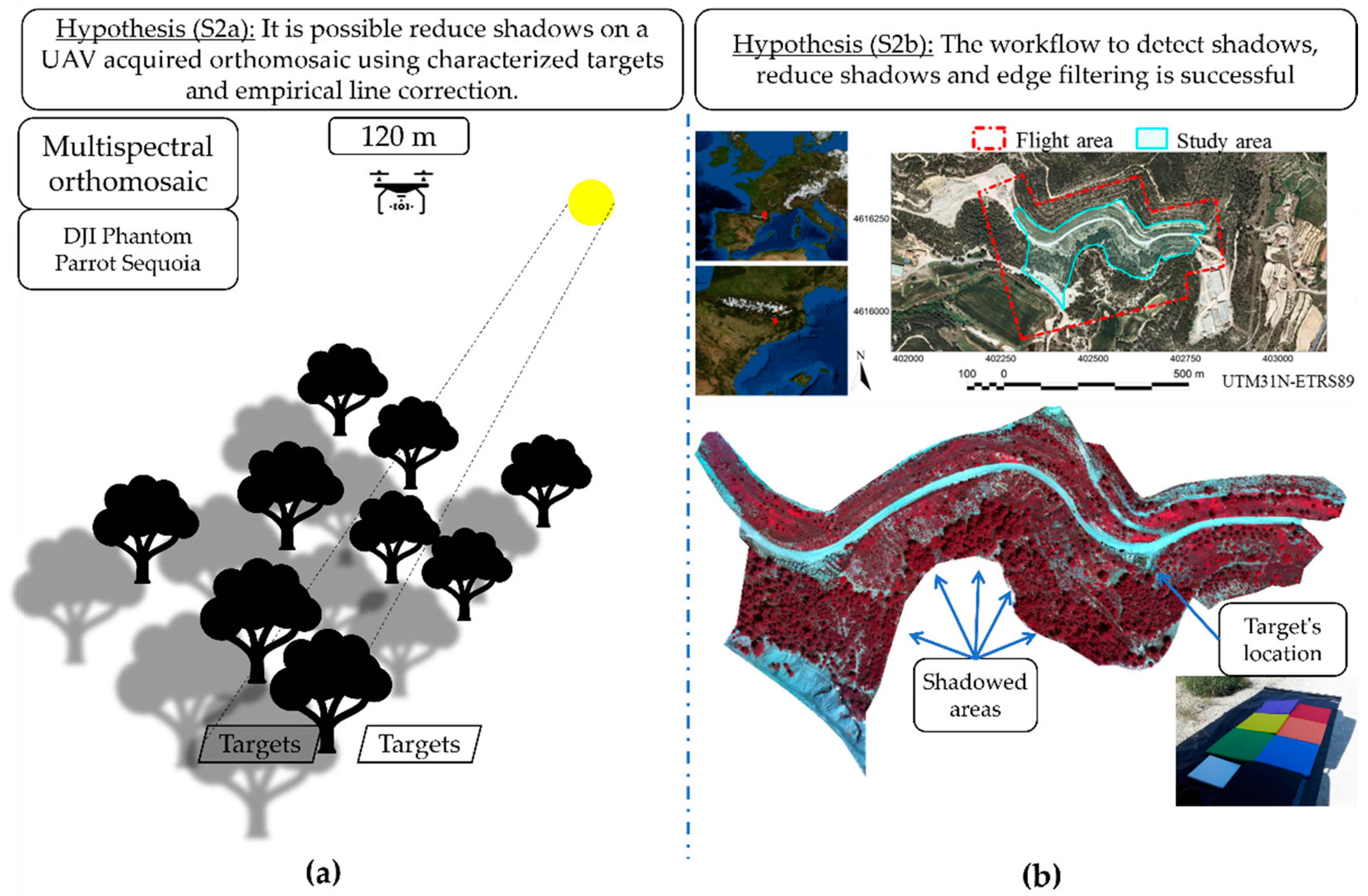
2.1. Experiment Conceptualization and Materials
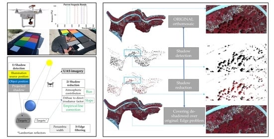
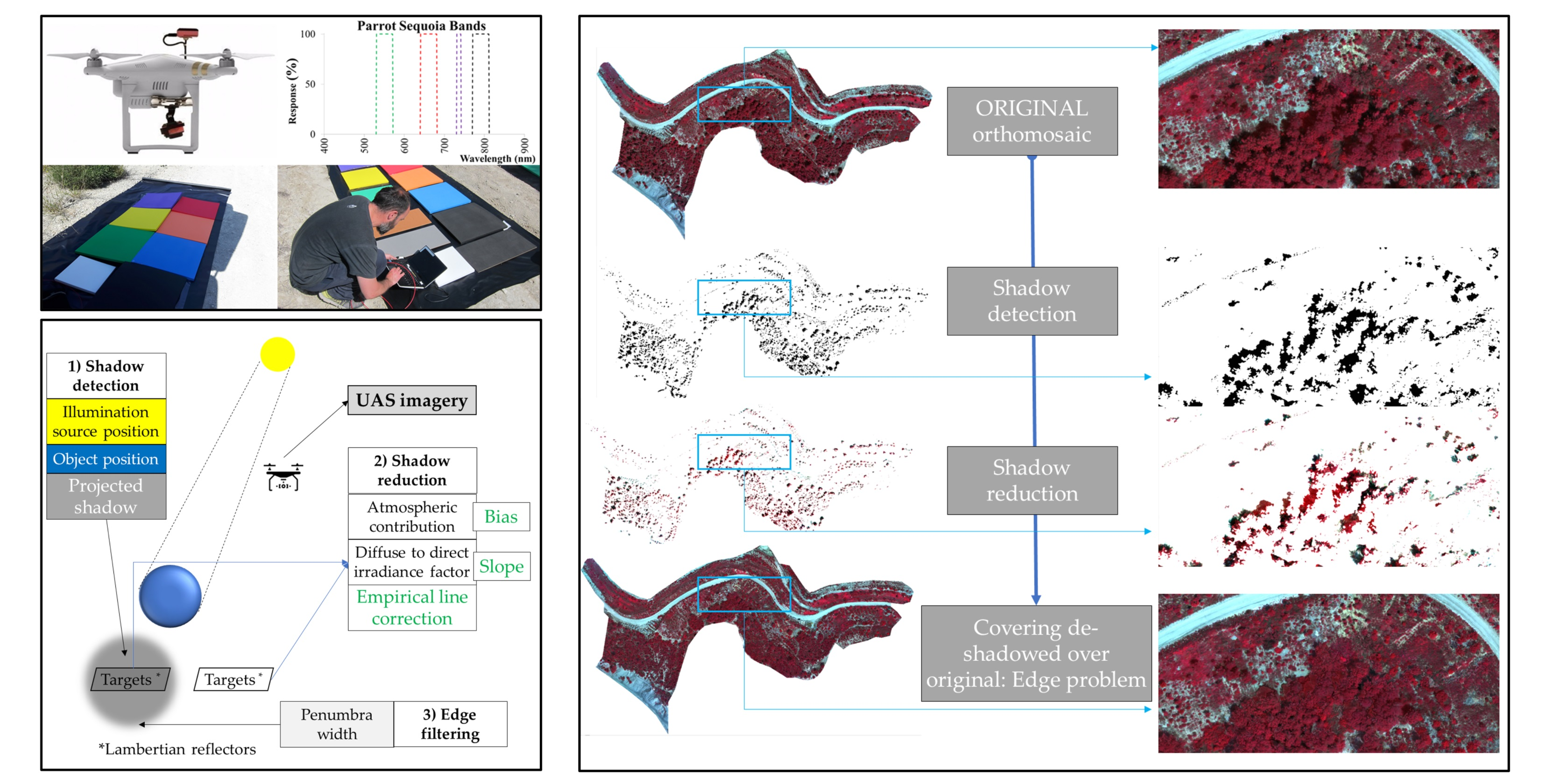
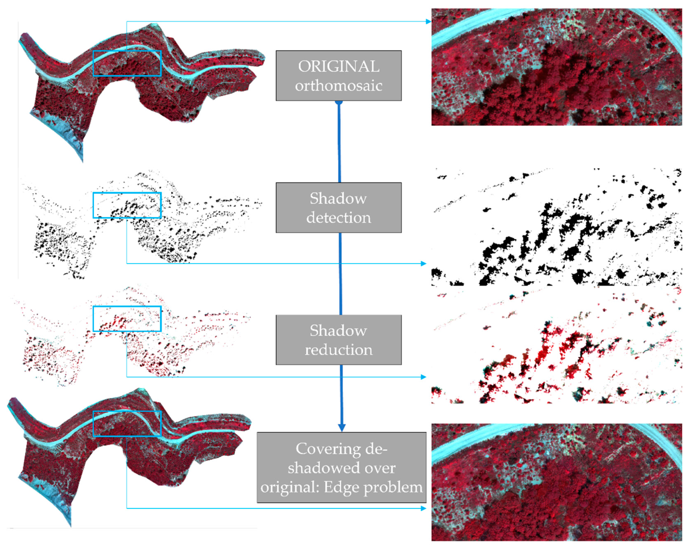
2.2. Methods: Shadow Detection, Shadow Reduction, Edge Filtering
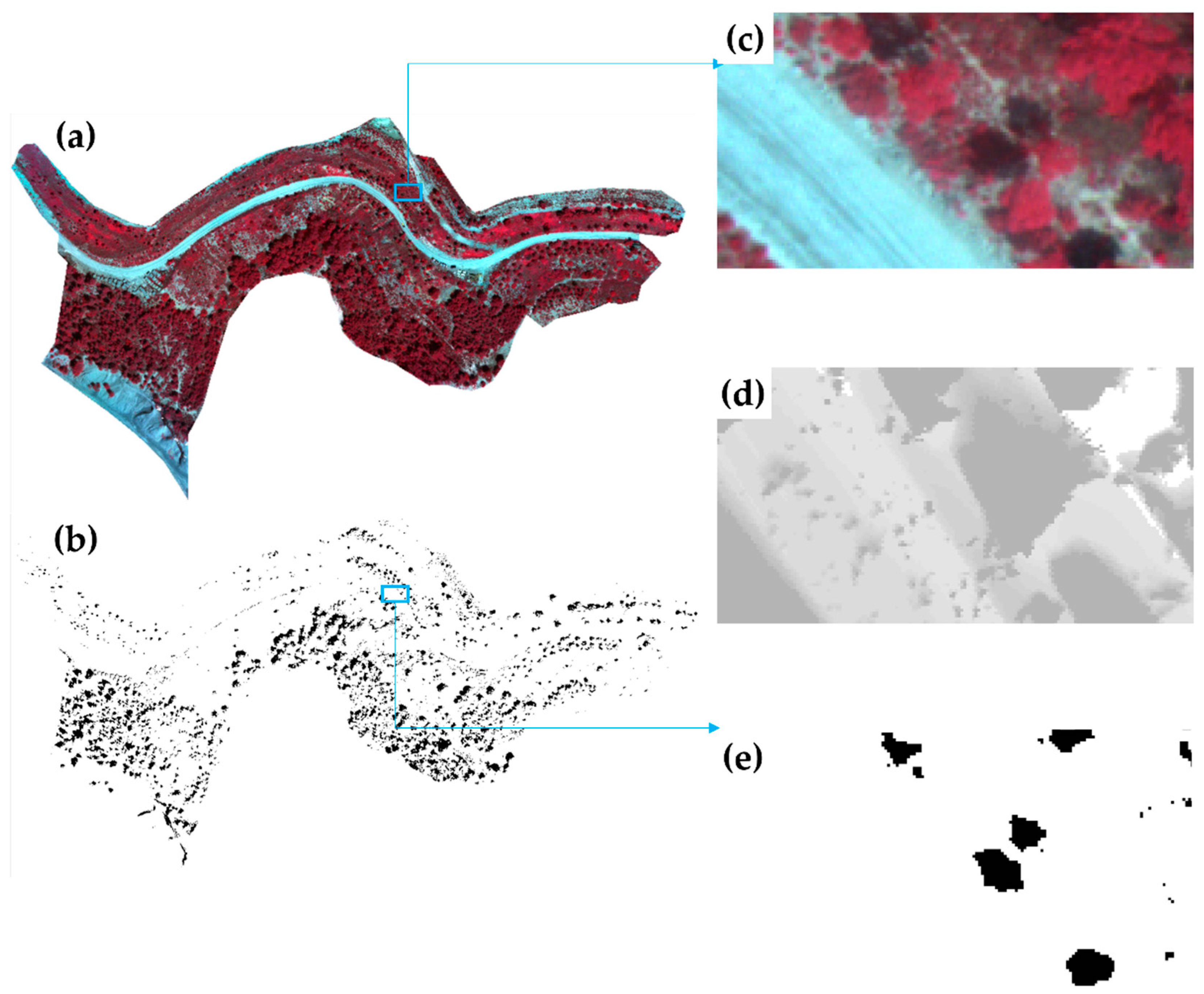
2.2.1. Shadow Detection
2.2.2. Shadow Reduction
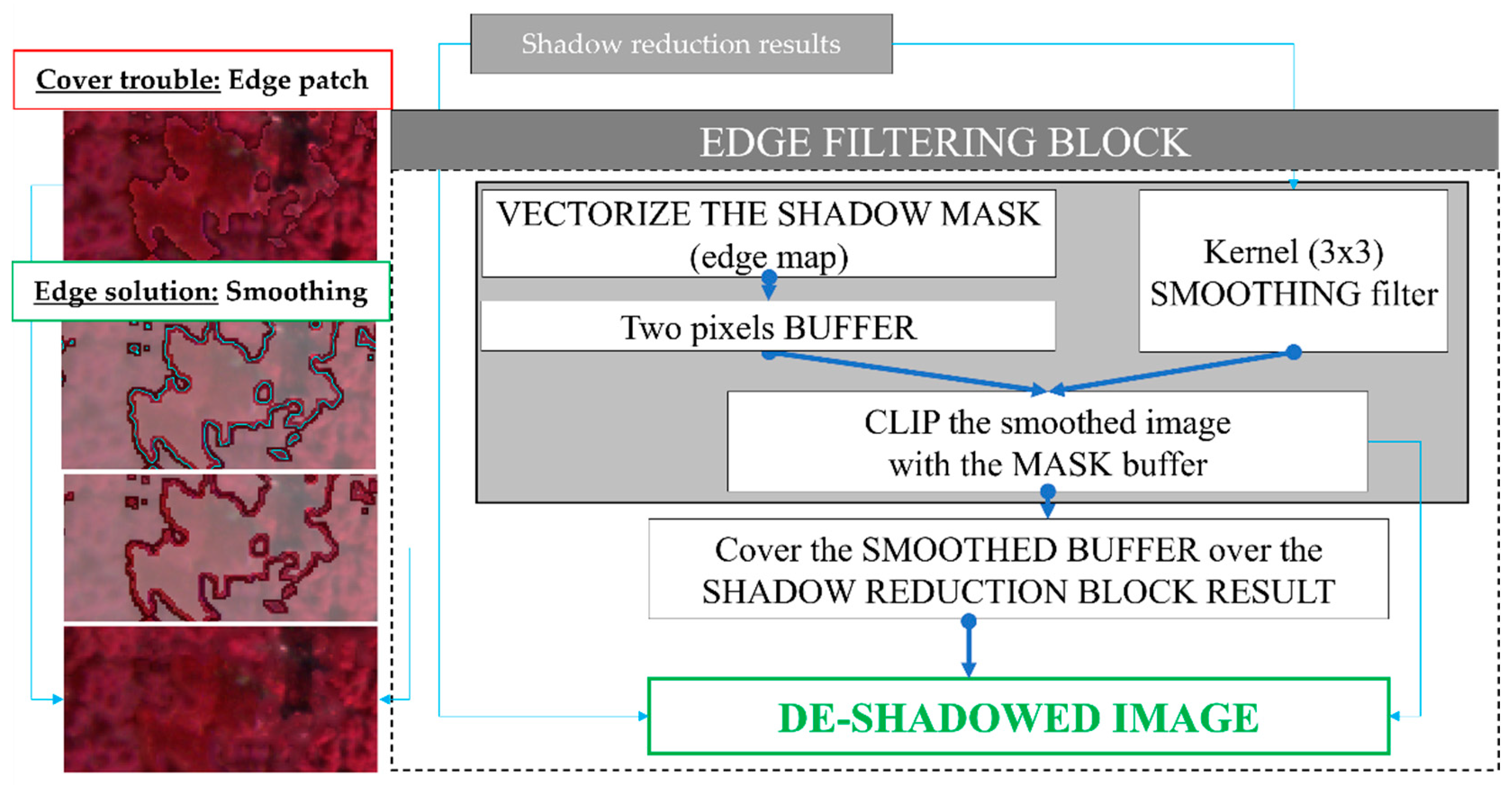
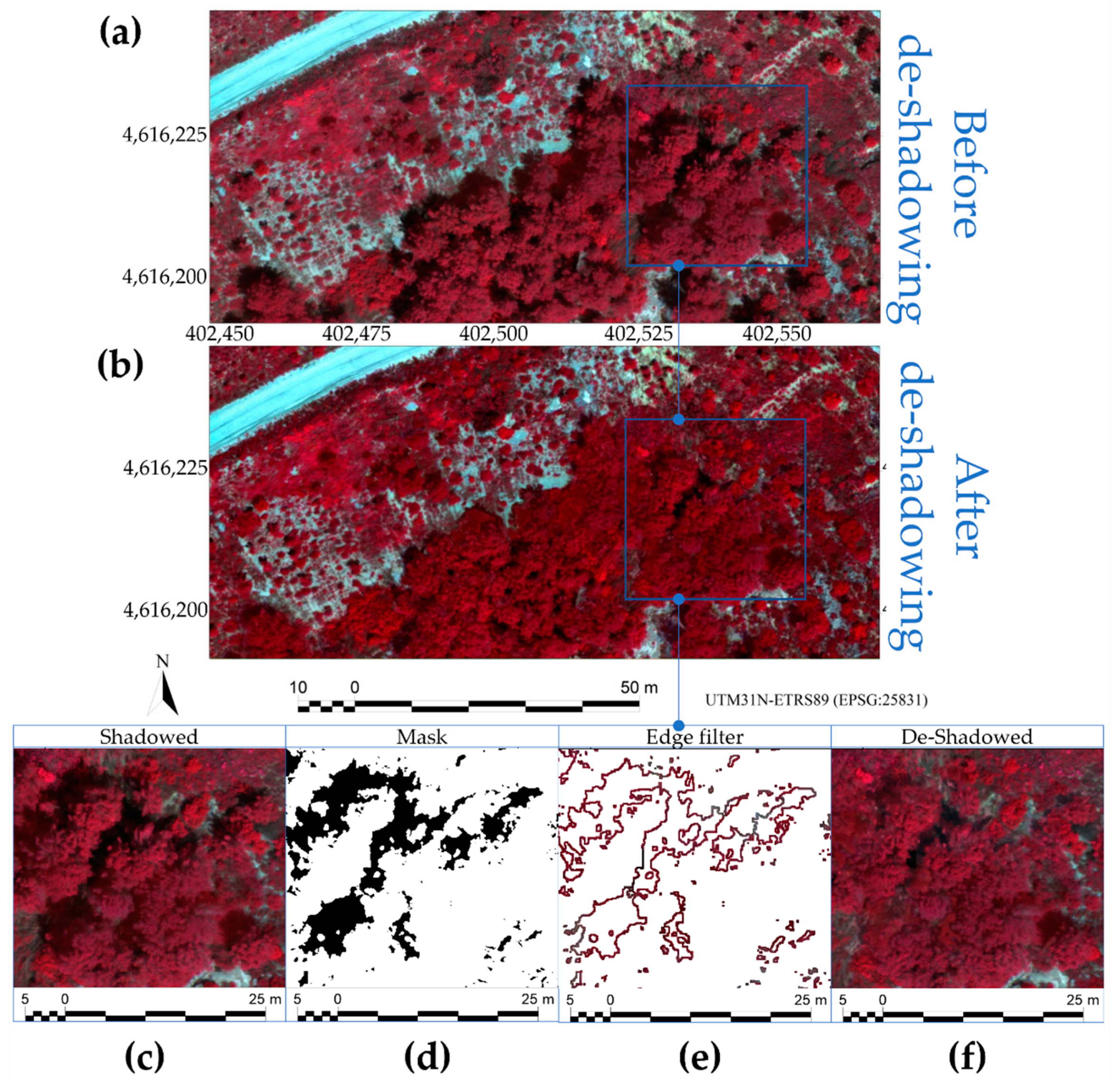
2.2.3. Edge Filtering
2.3. Methods: Statistical Data Analysis
3. Results
4. Discussion
5. Conclusions
Author Contributions
Funding
Institutional Review Board Statement
Informed Consent Statement
Conflicts of Interest
References
- Adler-Golden, S.; Matthew, M.W.; Anderson, G.P.; Felde, G.W.; Gardner, J.A. An Algorithm for De-Shadowing Spectral Imagery. Proc. SPIE Imaging Spectrom. 2002, VIII 4816, 203–210. [Google Scholar] [CrossRef]
- Nicodemus, F.E.; Richmond, J.C.; Hsia, J.J. Geometrical Considerations and Nomenclature for Reflectance; National Bureau of Standards, US Department of Commerce: Washington, DC, USA, 1977. Available online: http://graphics.stanford.edu/courses/cs448-05-winter/papers/nicodemus-brdf-nist.pdf (accessed on 1 August 2021).
- Milton, E.J.; Schaepmann, M.E.; Anderson, K.; Kneubühler, M.; Fox, N. Progress in field spectroscopy. Remote Sens. Environ. 2009, 113, S92–S109. [Google Scholar] [CrossRef] [Green Version]
- Teillet, P.M.; Guindon, B.; Goodenough, D.G. On the slope-aspect correction of multispectral scanner data. Can. J. Remote Sens. 1982, 8, 84–106. [Google Scholar] [CrossRef] [Green Version]
- Pons, X.; Solé-Sugrañes, L. A simple radiometric correction model to improve automatic mapping of vegetation from multispectral satellite data. Remote Sens. Environ. 1994, 45, 317–332. [Google Scholar] [CrossRef]
- Pons, X.; Pesquer, L.; Cristóbal, J.; González-Guerrero, O. Automatic and improved radiometric correction of Landsat imagery using reference values from MODIS surface reflectance images. Int. J. Appl. Earth Obs. Geoinf. 2014, 33, 243–254. [Google Scholar] [CrossRef] [Green Version]
- Riaño, D.; Chuvieco, E.; Salas, J.; Aguado, I. Assessment of different topographic corrections in Landsat-TM data for mapping vegetation types. IEEE Trans. Geosci. Remote Sens. 2003, 41, 1056–1061. [Google Scholar] [CrossRef] [Green Version]
- Richter, R.; Kellenberger, T.; Kaufmann, H. Comparison of topographic correction methods. Remote Sens. 2009, 1, 184–196. [Google Scholar] [CrossRef] [Green Version]
- Zhu, Z.; Woodcock, C.E. Object-based cloud and cloud shadow detection in Landsat imagery. Remote Sens. Environ. 2012, 118, 83–94. [Google Scholar] [CrossRef]
- Zhu, Z.; Woodcock, C.E. Automated cloud, cloud shadow, and snow detection in multitemporal Landsat data: An algorithm designed specifically for monitoring land cover change. Remote Sens. Environ. 2014, 152, 217–234. [Google Scholar] [CrossRef]
- Aeronautics and Space Administration (NASA). MODIS Web. Available online: https://modis.gsfc.nasa.gov/ (accessed on 1 August 2021).
- National Oceanic and Atmospheric Administration (NOAA). Advanced Very High Resolution Radiometer—AVHRR. Available online: https://www.avl.class.noaa.gov/release/data_available/avhrr/index.htm (accessed on 1 August 2021).
- Aeronautics and Space Administration (NASA). Landsat Data Continuity Mission (LDCM). Available online: https://www.nasa.gov/mission_pages/landsat/main/index.html (accessed on 1 August 2021).
- European Space Agency (ESAa). ESA Sentinel Online. Sentinel-2 Mission. Available online: http://www.esa.int/Our_Activities/Observing_the_Earth/Copernicus/Sentinel-2 (accessed on 1 August 2021).
- DigitalGlobe. Satellite Information. Available online: https://www.digitalglobe.com/resources/satellite-information (accessed on 1 August 2021).
- Fernández-Renau, A.; Gómez, J.A.; de Miguel, E. The INTA AHS System. Proc. SPIE 2005. [Google Scholar] [CrossRef]
- Jiménez, M.; Díaz-Delgado, R.; Vaughan, P.; De Santis, A.; Fernández-Renau, A.; Prado, E.; Gutiérrez de la Cámara, O. Airborne hyperspectral scanner (AHS) mapping capacity simulation for the Doñana biological reserve scrublands. In Proceedings of the 10th International Symposium on Physical Measurements and Signatures in Remote Sensing, Davos, Switzerland, 12–14 March 2007; Schaepman, M., Liang, S., Groot, N., Kneubühler, M., Eds.; Available online: http://www.isprs.org/proceedings/XXXVI/7-C50/papers/P81.pdf (accessed on 28 October 2017).
- Itres Research Ltd. Compact Airborne Spectrographic Imager (CASI-1500H). Available online: https://itres.com/wp-content/uploads/2019/09/CASI1500.pdf (accessed on 1 August 2021).
- Leica Geosystems. Leica DMCII Airborne Digital Camera. Available online: https://leica-geosystems.com/products/airborne-systems/imaging-sensors/leica-dmciii (accessed on 1 August 2021).
- Chen, Y.; Wen, D.; Jing, L.; Shi, P. Shadow information recovery in urban areas from very high resolution satellite imagery. Int. J. Remote Sens. 2007, 28, 3249–3254. [Google Scholar] [CrossRef]
- Dare, P.M. Shadow analysis in high-resolution satellite imagery of urban areas. PE&RS 2005, 71, 169–177. [Google Scholar] [CrossRef] [Green Version]
- Richter, R.; Muller, A. De-shadowing of satellite/airborne imagery. Int. J. Remote Sens. 2005, 26, 3137–3148. [Google Scholar] [CrossRef]
- Arévalo, V.; González, J.; Ambrosio, G. Shadow detection in colour high-resolution satellite images. Int. J. Remote Sens. 2008, 29, 1945–1963. [Google Scholar] [CrossRef]
- MicaSense. MicaSense RedEdge™ 3 Multispectral Camera User Manual; MicaSense, Inc.: Seattle, WA, USA, 2015; p. 33. Available online: https://support.micasense.com/hc/en-us/article_attachments/204648307/RedEdge_User_Manual_06.pdf (accessed on 1 August 2021).
- Parrot Drones. Parrot Sequoia Technical Specifications. 2018. Available online: https://www.parrot.com/global/parrot-professional/parrot-sequoia#technicals (accessed on 1 August 2021).
- Mapir. Specifications. 2021. Available online: https://www.mapir.camera/pages/survey3-cameras#specs (accessed on 1 August 2021).
- SAL Engineering. MAIA—The Multispectral Camera. 2021. Available online: https://www.salengineering.it/public/en/p/maia.asp (accessed on 1 August 2021).
- Markelin, L.; Simis, S.G.H.; Hunter, P.D.; Spyrakos, E.; Tyler, A.N.; Clewley, D.; Groom, S. Atmospheric Correction Performance of Hyperspectral Airborne Imagery over a Small Eutrophic Lake under Changing Cloud Cover. Remote Sens. 2017, 9, 2. [Google Scholar] [CrossRef] [Green Version]
- Salvador, E.; Cavallaro, A.; Ebrahimi, T. Shadow identification and classification using invariant color models. In Proceedings of the 2001 IEEE International Conference on Acoustics, Speech, and Signal Processing, Salt Lake City, UT, USA, 7–11 May 2001; Volume 3, pp. 1545–1548. [Google Scholar] [CrossRef] [Green Version]
- Shahtahmassebi, A.; Yang, N.; Wang, K.; Moore, N.; Shen, Z. Review of shadow detection and de-shadowing methods in remote sensing. Chinese Geogr. Sci. 2013, 23, 403–420. [Google Scholar] [CrossRef] [Green Version]
- Wu, T.; Zhang, L.; Huang, C. An analysis of shadow effects on spectral vegetation indices using a ground-based imaging spectrometer. In Proceedings of the 7th Workshop on Hyperspectral Image and Signal Processing: Evolution in Remote Sensing (WHISPERS), Tokyo, Japan, 2–5 June 2015; pp. 1–4. [Google Scholar] [CrossRef]
- Schaepman-Strub, G.; Schaepman, M.E.; Painter, T.H.; Dangel, S.; Martonchik, J.V. Reflectance quantities in optical remote sensing—definitions and case studies. Remote Sens. Environ. 2006, 103, 27–42. [Google Scholar] [CrossRef]
- Adeline, K.R.M.; Chen, M.; Briottet, X.; Pang, S.K.; Paparoditis, N. Shadow detection in very high spatial resolution aerial images: A comparative study. ISPRS J. Photogramm. 2013, 80, 21–38. [Google Scholar] [CrossRef]
- Honkavaara, E.; Saari, H.; Kaivosoja, J.; Pölönen, I.; Hakala, T.; Litkey, P.; Mäkynen, J.; Pesonen, L. Processing and Assessment of Spectrometric, Stereoscopic Imagery Collected Using a Lightweight UAV Spectral Camera for Precision Agriculture. Remote Sens. 2013, 5, 5006–5039. [Google Scholar] [CrossRef] [Green Version]
- Wang, C.; Myint, S.W. A Simplified Empirical Line Method of Radiometric Calibration for Small Unmanned Aircraft Systems-Based Remote Sensing. IEEE JSTARS 2015, 8, 1876–1885. [Google Scholar] [CrossRef]
- Padró, J.C.; Pons, X.; Aragonés, D.; Díaz-Delgado, R.; García, D.; Bustamante, J.; Pesquer, L.; Domingo-Marimon, C.; González-Guerrero, O.; Cristóbal, J.; et al. Radiometric Correction of Simultaneously Acquired Landsat-7/Landsat-8 and Sentinel-2A Imagery Using Pseudoinvariant Areas (PIA): Contributing to the Landsat Time Series Legacy. Remote Sens. 2017, 9, 1319. [Google Scholar] [CrossRef] [Green Version]
- Padró, J.C.; Muñoz, F.J.; Avila, L.A.; Pesquer, L.; Pons, X. Radiometric Correction of Landsat-8 and Sentinel-2A Scenes Using Drone Imagery in Synergy with Field Spectroradiometry. Remote Sens. 2018, 10, 1687. [Google Scholar] [CrossRef] [Green Version]
- Padró, J.C.; Carabassa, V.; Balagué, J.; Brotons, L.; Alcañiz, J.M.; Pons, X. Monitoring opencast mine restorations using Unmanned Aerial System (UAS) imagery. Sci. Total Environ. 2019, 657, 1602–1614. [Google Scholar] [CrossRef] [PubMed]
- Pons, X.; Padró, J.C. An Empirical Approach on Shadow Reduction of UAV Imagery in Forests. In Proceedings of the IGARSS 2019–2019 IEEE International Geoscience and Remote Sensing Symposium, Yokohama, Japan, 28 July–2 August 2019; pp. 2463–2466. [Google Scholar] [CrossRef]
- Bareth, G.; Aasen, H.; Bendig, J.; Gnyp, M.; Bolten, A.; Jung, A.; Michels, R.; Soukkamäki, J. Low-weight and UAV-based Hyperspectral Full-frame Cameras for Monitoring Crops: Spectral Comparison with Portable Spectroradiometer. PFG 2015, 1, 69–79. [Google Scholar] [CrossRef]
- Smith, G.M.; Milton, E.J. The use of the empirical line method to calibrate remotely sensed data to reflectance. Int. J. Remote Sens. 1999, 20, 2653–2662. [Google Scholar] [CrossRef]
- Perry, E.M.; Warner, T.; Foote, P. Comparison of atmospheric modelling versus empirical line fitting for mosaicking HYDICE imagery. Int. J. Remote Sens. 2000, 21, 799–803. [Google Scholar] [CrossRef]
- Karpouzli, E.; Malthus, T. The empirical line method for the atmospheric correction of IKONOS imagery. Int. J. Remote Sens. 2003, 24, 1143–1150. [Google Scholar] [CrossRef]
- Padró, J.C.; Muñoz, F.J.; Planas, J.; Pons, X. Comparison of four UAV georeferencing methods for environmental monitoring purposes focusing on the combined use with airborne and satellite remote sensing platforms. IJAEO 2019, 79, 130–140. [Google Scholar] [CrossRef]
- Photonic Solutions. USB200+ Data Sheet. OceanOptics; Ocean Optics, Inc.: Dunedin, FL, USA, 2006; Available online: https://www.photonicsolutions.co.uk/upfiles/USB2000PlusSpectrometerDatasheetLG14Jun18.pdf (accessed on 1 August 2021).
- European Union Aviation Safety Agency (EASA). Drones—Regulatory Framework Background. 2019. Available online: https://www.easa.europa.eu/easa-and-you/civil-drones-rpas/drones-regulatory-framework-background (accessed on 1 August 2021).
- Pons, X. MiraMon. Geographic Information System and Remote Sensing Software; Version 8.1j; Centre de Recerca Ecològica i Aplicacions Forestals, CREAF: Bellaterra, Spain, 2019; Available online: https://www.miramon.cat/Index_usa.htm (accessed on 1 August 2021)ISBN 84-931323-4-9.


| Date | 27 April 2018 |
|---|---|
| First photogram capture time (UTC) | 10:36:33 |
| Last photogram capture time (UTC) | 10:46:23 |
| Flight height Above Ground Level (m) | 90 |
| Number of photograms (x4 = bands) | 623 (2492) |
| Planned along-track overlapping (%) | 90 |
| Planned across-track overlapping (%) | 85 |
| Latitude of the center of the whole scene (°) | 41°41′31.29″ N |
| Longitude of the center of the whole scene (°) | 1°49′43.18″ E |
| Sun azimuth at central time of flight (°) | 146.50 |
| Sun elevation at central time of flight (°) | 58.37 |
| FWHM (nm) | Size (mm) | Weight (g) | Design | Manufacturer/Model |
|---|---|---|---|---|
| 1.26 | 89.1 × 63.3 × 34.4 | 190 | Czerny-Turner | OceanOptics USB2000+ |
| Input Focal Length (mm) | Fiber optic FOV (°) | Sampling interval (nm) | Sensor CCD samples | Grating #2 Spectral range (nm) |
| 42 | 25 | 0.3 | 2048 | 340–1030 |
| Expanded Dynamic Range (DN) | Size (mm) | Weight (g) | Sensor Type | Manufacturer-Model |
|---|---|---|---|---|
| 0–65,535 | 59 × 41 × 28 | 72 | CMOS | Parrot Sequoia |
| Raw radiometric resolution (bits) | Field of View (°) | Input Focal Length (mm) | Pixel size (µm) | Sensor size (pixels) |
| 10 | 47.5 | 3.98 | 3.75 × 3.75 | 1280 × 960 |
| #1 Blue FWHM (nm) | #2 Green FWHM (nm) | #3 Red FWHM (nm) | #4 Red-edge FWHM (nm) | #5 NIR FWHM (nm) |
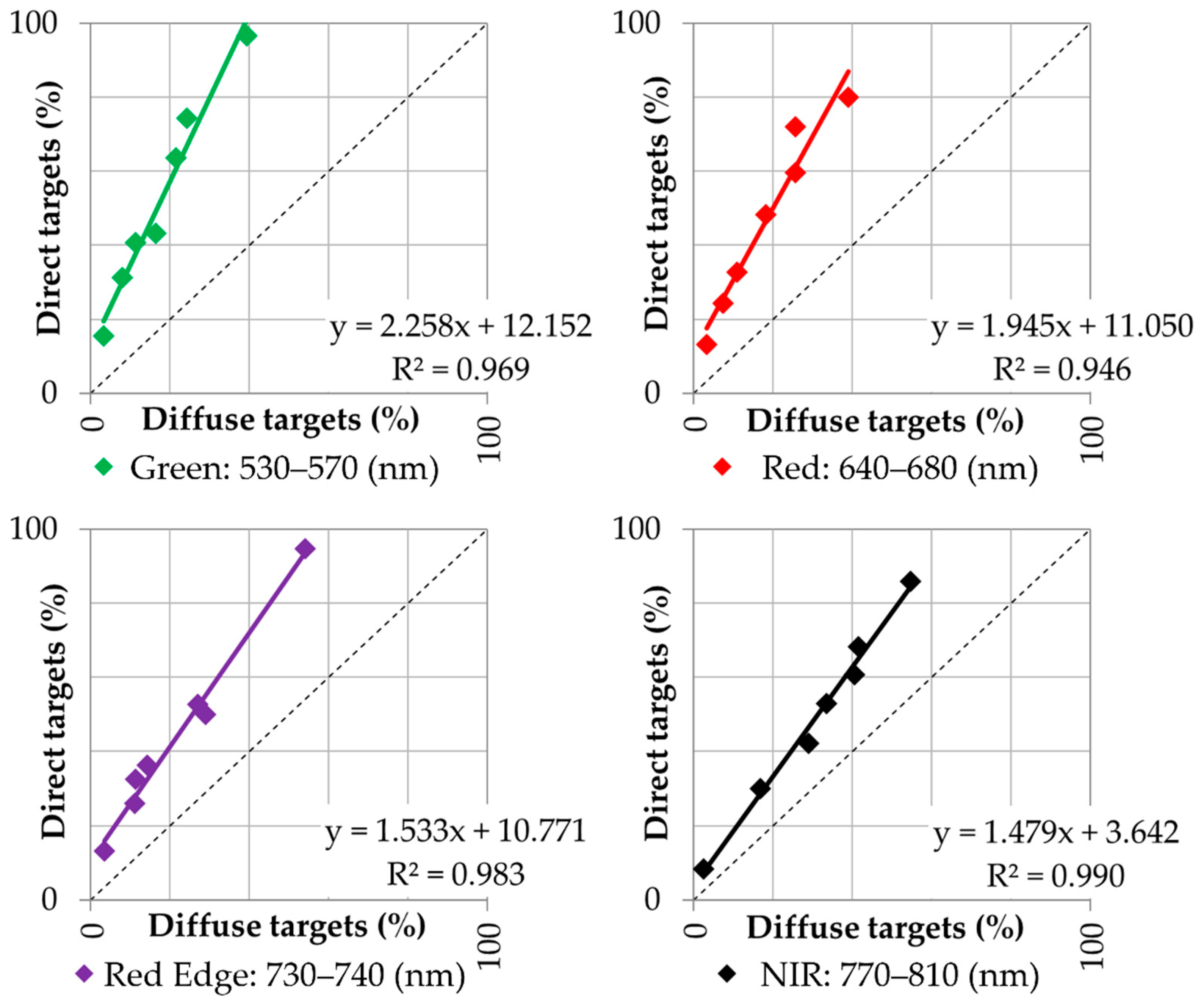
| No blue band | 530–570 | 640–680 | 730–740 | 770–810 |
| Parrot Sequoia Bands | R2 | Slope | Bias |
|---|---|---|---|
| Green: 530–570 (nm) | 0.969 | 2.258 | 12.152 |
| Red: 640–680 (nm) | 0.946 | 1.945 | 11.050 |
| Red Edge: 730–740 (nm) | 0.983 | 1.533 | 10.771 |
| NIR: 770–810 (nm) | 0.990 | 1.479 | 3.642 |
Publisher’s Note: MDPI stays neutral with regard to jurisdictional claims in published maps and institutional affiliations. |
© 2021 by the authors. Licensee MDPI, Basel, Switzerland. This article is an open access article distributed under the terms and conditions of the Creative Commons Attribution (CC BY) license (https://creativecommons.org/licenses/by/4.0/).
Share and Cite
Pons, X.; Padró, J.-C. An Operational Radiometric Correction Technique for Shadow Reduction in Multispectral UAV Imagery. Remote Sens. 2021, 13, 3808. https://doi.org/10.3390/rs13193808
Pons X, Padró J-C. An Operational Radiometric Correction Technique for Shadow Reduction in Multispectral UAV Imagery. Remote Sensing. 2021; 13(19):3808. https://doi.org/10.3390/rs13193808
Chicago/Turabian StylePons, Xavier, and Joan-Cristian Padró. 2021. "An Operational Radiometric Correction Technique for Shadow Reduction in Multispectral UAV Imagery" Remote Sensing 13, no. 19: 3808. https://doi.org/10.3390/rs13193808
APA StylePons, X., & Padró, J.-C. (2021). An Operational Radiometric Correction Technique for Shadow Reduction in Multispectral UAV Imagery. Remote Sensing, 13(19), 3808. https://doi.org/10.3390/rs13193808